
Instance Segmentation of Shrimp Based on Contrastive Learning
by
 ,
,
Heng Zhou
1 ,
,
Sung Hoon Kim
1,
Sang Cheol Kim
2,
Cheol Won Kim
3,
Seung Won Kang
4 and
Hyongsuk Kim
2,* 1
Division of Electronics and Information Engineering, Jeonbuk National University, Jeonju 54896, Republic of Korea
2
Core Research Institute of Intelligent Robots, Jeonbuk National University, Jeonju 54896, Republic of Korea
3
Division of Aquatic Life Culturing, Korea National University of Agriculture and Fisheries, Jeonju 54874, Republic of Korea
4
Daesang Aquaculture Trout Association Corporation, Taean 32158, Republic of Korea
*
Author to whom correspondence should be addressed.
Appl. Sci. 2023, 13(12), 6979; https://doi.org/10.3390/app13126979
Submission received: 2 May 2023
/
Revised: 29 May 2023
/
Accepted: 7 June 2023
/
Published: 9 June 2023
Abstract
:Shrimp farming has traditionally served as a crucial source of seafood and revenue for coastal countries. However, with the rapid development of society, conventional small-scale manual shrimp farming can no longer meet the increasing demand for rapid growth. As a result, it is imperative to continuously develop automation technology for efficient large-scale shrimp farming. Smart shrimp farming represents an innovative application of advanced technologies and management practices in shrimp aquaculture to expand the scale of production. Nonetheless, the use of these new technologies is not without difficulties, including the scarcity of public datasets and the high cost of labeling. In this paper, we focus on the application of advanced computer vision techniques to shrimp farming. To achieve this objective, we first establish a high-quality shrimp dataset for training various deep learning models. Subsequently, we propose a method that combines unsupervised learning with downstream instance segmentation tasks to mitigate reliance on large training datasets. Our experiments demonstrate that the method involving contrastive learning outperforms the direct fine-tuning of an instance segmentation model for shrimp in instance segmentation tasks. Furthermore, the concepts presented in this paper can extend to other fields that utilize computer vision technologies.
1. Introduction
Shrimp farming is an aquaculture practice that involves cultivating shrimp in controlled aquatic environments, such as ponds, raceways, and tanks. In recent years, shrimp farming has become a significant source of seafood and income for many coastal countries worldwide. With the rapid development of technology and the rise of labor costs, traditional small-scale manual shrimp farming practices can no longer meet the increasing demand. The latest developments in shrimp farming are focused on sustainability, productivity, and efficiency. Smart shrimp farming is an innovative application of advanced technologies and innovative management practices in shrimp aquaculture aimed at enhancing these three aspects [1]. It uses the latest artificial intelligence techniques to assist farmers in managing the entire shrimp aquaculture process [2,3,4,5]. These advanced techniques allow for the real-time monitoring of shrimp growth and water quality, feeding schedule management, and disease outbreak detection. Computer vision techniques can automate various aspects of shrimp farming using cameras and image processing or deep learning methods [6]. For instance, instance segmentation methods can accurately count the number of shrimp and estimate size information [3,4], which helps optimize feeding schedules and improve harvest yields. Shrimp tracking can be used to monitor shrimp health by detecting their movement and behavior, enabling early intervention to prevent disease outbreaks.
However, the performance of these techniques heavily relies on the quality of the data used to train the deep learning models. At present, there is no high-quality public shrimp dataset available in the research community, to the best of our knowledge. This is one of the major challenges in applying computer vision technology to enhance shrimp farming. Moreover, even if a large number of shrimp images are collected, image annotation is another time-consuming and labor-intensive task. The existing public datasets in computer vision communities do not include shrimp categories, making it necessary to train deep learning models for shrimp from scratch.
This paper proposes an innovative approach to bridge the gap between computer vision technology and shrimp farming by using unsupervised learning to train deep learning models for shrimp. Specifically, this paper suggests using a contrastive learning (CL) mechanism [7] to train the feature extractor and obtain visual representations of shrimp. These visual representations can benefit downstream computer vision tasks such as shrimp object detection, tracking, and instance segmentation. This paper fine-tunes five state-of-the-art contrastive learning models, namely MoCov1 [8], MoCov2 [9], MoCov3 [10], SimCLR [11], and Byol [12], using a shrimp dataset collected by our team. All five of these models take ResNet-50 [13] as an encoder architecture in their original papers and differ in the methods of data augmentation and training methods. This paper focuses on fine-tuning the ResNet-50 for shrimp without label information and then transferring the visual representations to the instance segmentation task. Therefore, we use the optimal setting to train our models, according to the original papers, and do not delve into the ideas behind the five contrastive learning models. For the instance segmentation task, we replace the original ResNet-50 in the Mask R-CNN [14] architecture with the pre-trained one, trained using the contrastive learning mechanism, and fine-tune the rest of the modules by supervised learning. Since the pre-trained ResNet-50 model has a good ability to extract feature representations of shrimp, the customized Mask R-CNN needs fewer samples with label information to fine-tune, but has a better performance compared to common fine-tuning methods.
We collected approximately 10k shrimp images to train the five contrastive learning models used in this study. A sample of these images is presented in Figure 1. There are five video sequences recording the movements of the shrimp. We recorded five video sequences of shrimp movements, each of which varied in illumination, individual shrimp, shrimp density, and moving speed, providing a diverse set of data for training deep learning models. In particular, as shown in Figure 1, the first sequence has brighter lighting than the others. The second sequence has a few more shrimp than the first sequence and has a larger shrimp size than the third and fourth sequences. The fifth sequence has the fastest moving speed, while the fourth sequence has the largest shrimp density of all sequences. Therefore, each sequence has its own features, providing much diversity to adapt to real-world application scenarios. To fine-tune the instance segmentation task, we labeled 1000 shrimp images in COCO dataset [15] formats. We split the labeled dataset into training, validation, and test datasets to assess the performance of the pre-trained contrastive learning models.
The experiments were conducted using the two datasets mentioned above. Firstly, approximately 10 k shrimp images were used to train each encoder (ResNet-50 [13]) with varying crop sizes. These encoders were then transferred to Mask R-CNN [14], and the modules, except the backbone, were retrained with the 1k labeled shrimp dataset. Additionally, the common fine-tuning methods were used to retrain Mask R-CNN using the same 1 k labeled shrimp dataset. To compare the performance of the encoders of contrastive learning models, we fine-tuned Mask R-CNN and our customized version using 20%, 40%, 60%, 80%, and 100% of the training dataset. The experimental results show that using the pre-training models from contrastive learning outperforms fine-tuning the original Mask R-CNN models directly. More importantly, the pre-training models from contrastive learning exhibit superior performance compared to the original backbone of Mask R-CNN, even when trained with small-scale datasets. The experimental results prove the effectiveness of unsupervised learning on the specific computer vision task, which can significantly reduce the labeling work in real applications while providing superior performance.
The contributions of this paper are summarized as follows:
- This paper contributes a high-quality, publicly available dataset of shrimp images, addressing the lack of such resources for computer vision applications in smart shrimp farming. In addition, this paper presents a labeled-instance segmentation shrimp dataset to support the development of deep learning methods in this domain. These contributions are expected to facilitate the advancement of computer vision technologies and their integration with smart shrimp farming practices.
- This paper provides a novel approach for combining unsupervised learning methods with shrimp instance segmentation. By utilizing unsupervised learning for completing instance segmentation tasks, the reliance on labeled data is significantly reduced, leading to reduced labeled costs for smart shrimp farming applications. Moreover, the methods presented in this paper have the potential to be extended and applied to other domains and applications beyond shrimp farming.
- This paper sets a new benchmark for shrimp instance segmentation in both supervised and unsupervised learning approaches. Additionally, we will make the shrimp datasets and pre-trained models for contrastive learning and Mask R-CNN publicly available for researchers and practitioners to use and further advance the field. Code is released at https://github.com/heng94/ShrimpInstanceSegmentation.git (accessed on 6 June 2023).
The remainder of this paper is structured as follows.
In Section 1, we provide background information on smart shrimp farming and discuss the benefits of combining unsupervised learning with this application. Section 2 gives an overview of the relevant literature on the use of computer vision techniques in shrimp farming and the progress made in contrastive learning. Next, in Section 3, we describe in detail the process of data collection and labeling, as well as the strategies used for training contrastive learning encoders and fine-tuning Mask R-CNN models. Section 4 contains the experimental results and analyses. Finally, Section 5 concludes the whole paper.
2. Related Works
2.1. Applications of Computer Vision in Shrimp Farming
Shrimp counting is a widely applied computer vision technology in the field of shrimp farming. The authors in [6] proposed an automatic shrimp counting method using the YOLO algorithm [16]. Their experiments were conducted on shrimp larvae with a low shrimp density and achieved a mean average precision (mAP) value of 96.83% and an average accuracy value of 76.48%. Similarly, in [17], the authors proposed the use of Mask R-CNN [14] for shrimp larvae counting. In contrast, ref. [6] proposed the use of the YOLOv4 [18] network with MobileNetv3 [19] for counting shrimp during the entire growth process. Despite the small and transparent body of the shrimp, their method achieved a precision of 92.12%, recall of 94.21%, F1 value of 93.15%, and mean average precision of 93.16%. Additionally, in [5], the authors proposed a hybrid recognition method that combined image enhancement strategies with the YOLOv4 deep learning method for detecting peeled shrimp in peeling processing. Through various image augmentation strategies, they concluded that YOLOv4 had the best detection performance. Several researchers have focused on shrimp recognition, and various deep learning models have been proposed for this purpose. Hu et al. [20] proposed ShrimpNet, a convolutional neural network (CNN) model that includes two CNN layers and two fully connected layers for shrimp recognition. However, the authors did not release their dataset containing six different categories of shrimp for further research. To address the problem of relying on handcrafted features, Liu et al. [21] proposed an improved version of ShrimpNet, which achieved an accuracy of 96.84%. Moreover, Liu et al. [22] proposed Deep-ShrimpNet, a model that classifies shrimp and performs quality evaluation. Thai et al. [4] proposed a deep learning network based on U-Net [23] to perform shrimp counting and evaluate shrimp density and size.
The aforementioned applications have the potential to significantly improve the efficiency of shrimp farming. However, they all rely on training deep learning networks with their own proprietary datasets. Furthermore, image labeling is a time-consuming and costly task for each application. Consequently, there is a lack of a standard and publicly available shrimp dataset for training these networks. This paper aims to address this gap by providing a comprehensive and public shrimp dataset that can be used for fundamental computer vision tasks such as recognition, object detection, and instance segmentation. Additionally, this paper proposes the integration of unsupervised learning methods to mitigate the reliance on labeled data during the training process.
2.2. Feature Representation Based on Contrastive Learning
Recently, computer vision communities have paid much more attention to unsupervised learning. Ref. [8] proposed a new unsupervised learning approach called momentum contrast (MoCo) for learning visual representations from unlabeled images. MoCo uses a momentum-based update rule to improve the efficiency and effectiveness of contrastive learning and achieved state-of-the-art performance on several downstream tasks, such as image recognition, object detection, and instance segmentation. Ref. [9] built upon the MoCo framework and proposed several improvements to the baseline MoCo method, including the use of larger batch sizes and stronger data augmentation. The authors show that these improvements lead to significant performance gains on several benchmark datasets. Ref. [11] proposed a simple framework called SimCLR for contrastive learning that combines several existing techniques, including data augmentation, negative sampling, and temperature scaling. Ref. [10] investigated the effectiveness of self-supervised learning for vision transformers, which are deep neural networks used for image recognition tasks. The authors compared several different self-supervised learning approaches and found that certain variants of contrastive learning perform well. Ref. [12] proposed a new self-supervised learning approach called Byol, which uses a two-network architecture to learn representations from unlabeled data. Ref. [24] proposed a new mutual contrastive learning approach that leverages both positive and negative examples during training. Ref. [25] proposed a new contrastive learning approach based on hyperbolic geometry, which is better suited for representing hierarchical data structures. The authors show that their method achieves state-of-the-art performance on several benchmark datasets that require the capture of hierarchical relationships, such as fine-grained classification and action recognition. Ref. [26] proposed a decentralized approach to unsupervised learning called DeepCluster-v2, which distributes the learning across multiple devices. This method achieved state-of-the-art performance on several benchmark datasets while also reducing the computational cost of training. Ref. [27] investigated the conditions under which contrastive learning is effective for visual representation learning. The authors found that contrastive learning works well in low-data regimes and when the dataset is diverse, but that it did not always outperform supervised learning methods.
Based on the progress of contrastive learning, Yu et al. [28] proposed a multi-view trajectory contrastive learning strategy to fully exploit the information contained in a whole trajectory and devise trajectory-level contrastive loss to explore the inter-frame information across whole trajectories. In a long-tailed image classification task, Wang et al. [29] investigated and adapted efficient supervised contrastive learning strategies, aiming to optimize image representations and address the challenge of class imbalance, to enhance classification accuracy for imbalanced data. Hou et al. [30] proposed a hyperspectral imagery classification algorithm based on contrast learning to solve the problem of limited label information in hyperspectral images. Taking inspiration from the successful applications of contrastive learning in various domains, this paper proposes to apply contrastive learning to the field of smart shrimp farming.
3. Methods
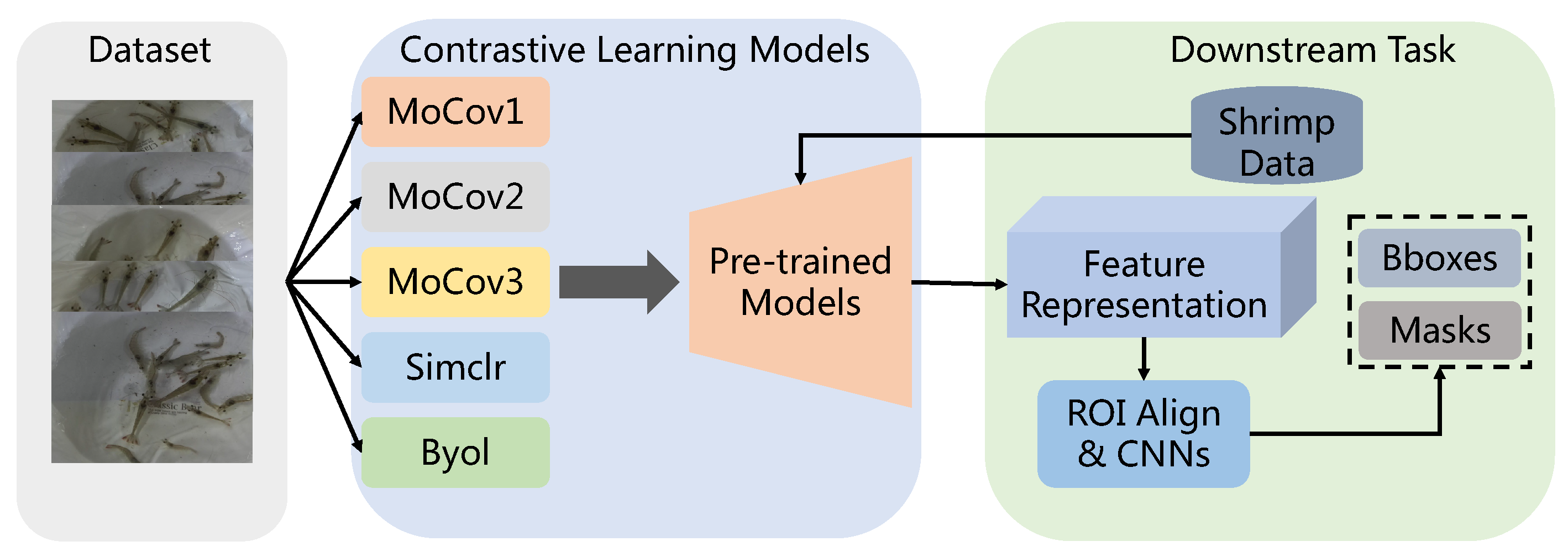
The architecture of this paper is illustrated in Figure 2, which comprises three main components: data collection, the training of contrastive learning models, and the fine-tuning of the downstream task. Firstly, we use the shrimp dataset which has no supervised information to retrain five contrastive learning models, obtaining the pre-trained models of shrimp. These pre-trained models serve as the backbones, and the rest of the modules of the Mask R-CNN model [14] are fine-tuned using these pre-trained models. Finally, the customized Mask R-CNN model produces bounding boxes and masks of shrimp. The following subsections provide detailed information on the three components.
3.1. Data Collection and Labeling
To collect shrimp images for this study, our team collaborated with a shrimp farm on Sinan Island, Republic of Korea. Due to the dirty water in the shrimp pool, it was not possible to take pictures of the shrimp directly. Instead, we removed the shrimp from the pool and placed them in a pot with clean water. We used the ZED 2 camera from STEREOLABS, a stereo camera that can produce video sequences with two different viewpoints. To ensure diversity in the dataset, we varied the settings when taking pictures, including illumination, shrimp density, shrimp size, and shrimp movement speed. After obtaining the video files, we used a script provided by the company to extract shrimp images. To build the training dataset for contrastive learning models, we adopted a strategy of keeping one image for every twenty images to remove similar images. Each image was then scaled to a width of 640 and a height of 480 to reduce the computational load of the deep learning models. The dataset contained approximately 10,000 images and was organized in the format of the ImageNet [31] dataset for ease of training. Since there was only one class (shrimp) in the dataset and the aim of training the contrastive learning models was to extract feature representations of shrimp, there was no validation or test dataset for these models. Hence, it is less meaningful to compare the performance of each contrastive learning model using a validation or test dataset. The performance comparison of the five models is reflected in downstream tasks.
For data labeling, we utilized the open-source annotation tool CVAT to facilitate the annotation of shrimp masks. The dataset contained a total of 1k images, which were extracted from other video sequences. This dataset was then divided into training, validation, and test sets with a ratio of 8:1:1. Since these two sets of data are completely separated, our experimental results are more compelling and impartial.
3.2. Contrastive Learning on Shrimp Feature Representations
Benefiting from the progress of contrastive learning [8,9,10,11,12,24,25,26,27], it is possible to train custom backbones for downstream tasks without relying on supervised information. In this paper, we train five state-of-the-art contrastive learning models—MoCov1, MoCov2, MoCov3, SimCLR, and Boyl—as backbones for shrimp instance segmentation. Since the main focus of this paper is on training pre-trained models for shrimp, this subsection only provides a brief introduction to these five models. For more information, readers can refer to the original papers.
MoCo series contrastive learning models are proposed in [8,9,10]. The main idea of MoCov1 [8] is to build a dynamic dictionary with a queue and a moving-averaged encoder and utilize contrastive loss to update the network. There are two encoders in MoCo architecture, where one encoder named q is used to extract features of the current query image, while another encoder named k is employed to obtain the features of the images in the dictionary constructed by the rest of the images in one mini-batch. For one image in a mini-batch, this image is randomly transformed by two different kinds of image augmentations, generating two images: and . is the query image. is the positive sample of while the rest of the images in this mini-batch are the negative samples of . Therefore, there are many negative pairs but only one positive pair in this mini-batch. and together with other images are sent to the encoders q and k to obtain feature maps, respectively. The parameter update of encoder q is achieved by gradient back-propagation, while the parameter update way of encoder k is momentum update, which is expressed in the following:
where and are the parameters of encoder k and encoder q, respectively. is a momentum coefficient. In back-propagation, the loss function is the contrastive loss, called NCELoss, which is
where is the output of encoder q, while and are the output of encoder k. is a temperature hyper-parameter. The value of this loss function becomes small when is similar to its positive sample and dissimilar to all other negative samples. MoCov2 [9] uses the same architecture as MoCov1 but differs in the methods of image augmentation. MoCov3 [10] primarily utilizes a vision transformer network (ViT) [32] as the encoder for contrastive learning while exploring the performances of different settings in the ViT network. However, since we aim to transfer the visual representations generated by contrastive learning models to shrimp instance segmentation, we replace ViT in MoCov3 with ResNet-50 while keeping the other settings consistent with MoCov3.
SimCLR [11] simplifies the contrastive learning architectures by removing the requirement for specialized networks or a memory bank. The differences between SimCLR and MoCo lie in the fact that SimCLR adds a learnable nonlinear transformation between the representation and the contrastive loss to improve the quality of the learned representations. Additionally, SimCLR shows that the composition of multiple data augmentation operations is crucial for contrastive learning, and it thus employs many other kinds of data augmentation. Byol [12] combines the benefits of both MoCo and SimCLR models and achieves a new state-of-the-art performance on many public datasets. Unlike MoCo, Byol trains an online network to predict the target network representation of the same image by using different augmentation methods. Furthermore, it updates the target network with a slow-moving average of the online network.
3.3. Shrimp Instance Segmentation Based on Contrastive Learning
In this subsection, we describe the method of combining the aforementioned contrastive learning models with the Mask R-CNN model [14] for shrimp instance segmentation. From a compositional perspective, the Mask R-CNN model consists of four modules: backbone, neck, RPN-head and RoI-head. Among these modules, the backbone plays a crucial role in determining the quality of feature representations. The conventional fine-tuning approach for a custom dataset involves training all four modules of the Mask R-CNN model based on a pre-trained model from public datasets. However, this approach often fails to achieve satisfactory performance, as the backbone may not be able to extract discriminative feature representations with the limited dataset.
Therefore, this paper proposes to train only the backbone, using unsupervised learning to minimize the labeling cost. Specifically, we train five different kinds of backbones using the five contrastive learning models described earlier, where the backbone network is the ResNet-50 [13]. Once we finish training the backbone, we fix its parameters and fine-tune the other three modules of the Mask R-CNN model. This fine-tuning approach offers several advantages. It can achieve better performance than the conventional fine-tuning method, and it is feasible even when the dataset size is limited.
4. Experimental Results
4.1. Implementation Details
Our implementation is based on the open-source toolbox MMSelfSup [33]. We conducted all experiments on the five state-of-the-art contrastive learning models using this toolbox. We followed the default settings in each configuration file except for the input size of the image. The default input size in the toolbox is 224, while we tested two different sizes, 244 and 480, because our shrimp image size was . Data augmentation and batch size are the two most important settings in training contrastive learning models. A larger batch size theoretically produces better experimental results. However, due to computational resource limitations, we set the batch size as 32 for all five contrastive learning models. Table 1 lists the data augmentations used for each model. We chose the ResNet-50 network as the encoder in all five contrastive learning models for the convenience of transferring it to Mask R-CNN as the backbone.
For instance, for the segmentation experiments, we kept all settings consistent for each contrastive learning model and supervised model, except the backbone. The input size was set as , and the batch size was 8. The initial learning rate was 0.01 and the training epoch was 96. The stochastic gradient descent (SGD) optimizer was employed in the network, and the common metrics from instance segmentation tasks, such as , , and were used to evaluate the performance. Average precision () was calculated by computing the precision and recall values at different intersections over union (IoU) thresholds, typically ranging from 0.5 to 0.95 with a step size of 0.05. , which is Average Precision at IoU 0.50, measures the average precision at an IoU threshold of 0.50. , which is Average Precision at IoU 0.75, calculates the average precision at an IoU threshold of 0.75. Both and are complementary metrics to , providing a more detailed evaluation of the model’s performance at specific IoU thresholds.
4.2. Contrastive Learning Results
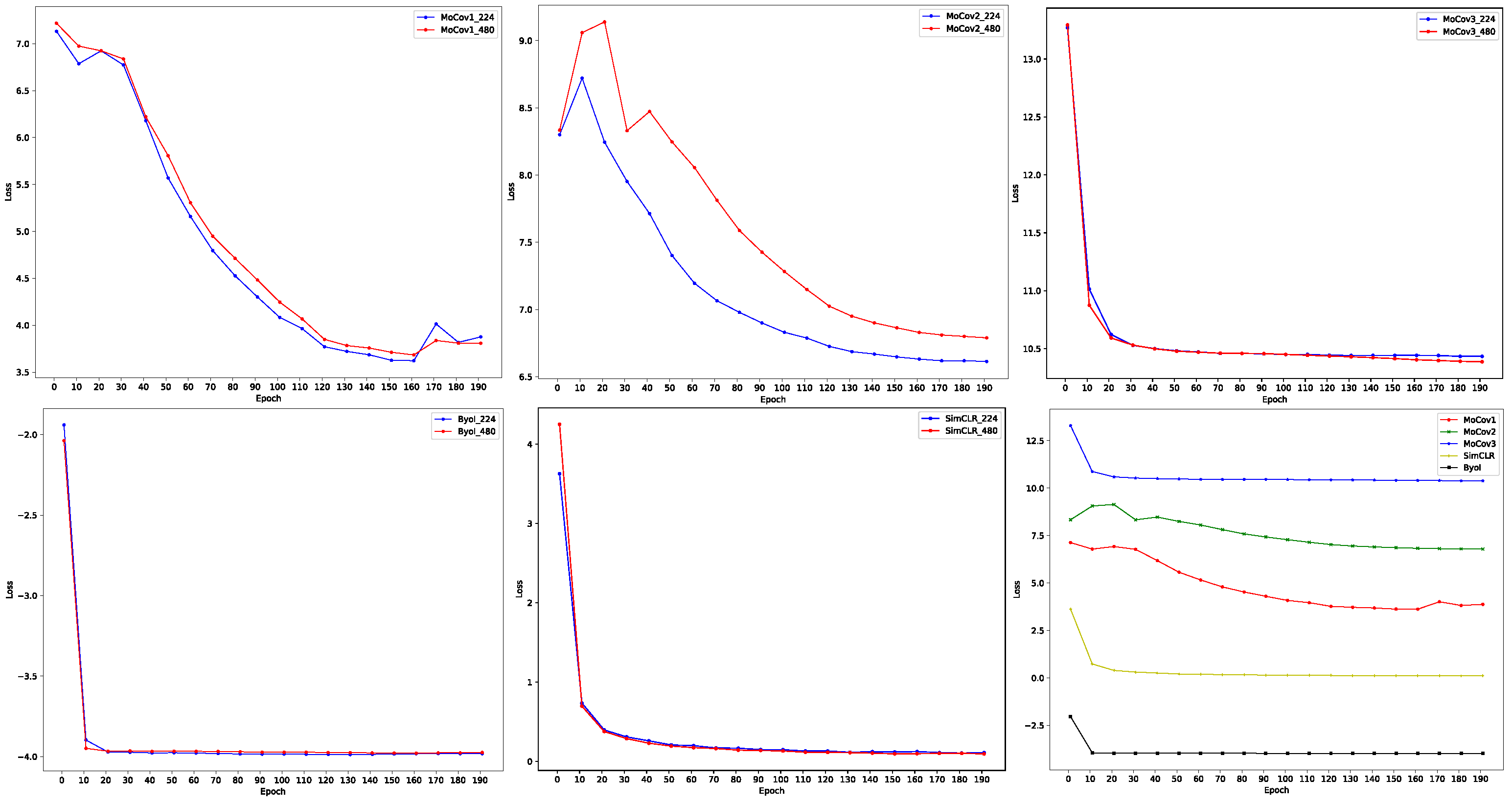
The training of contrastive learning models is typically referred to as a pre-text task, which is a self-supervised learning task aimed at learning visual representations. Its performance cannot be directly evaluated and must be assessed by testing the performance of downstream tasks. Evaluations of image classification tasks are a common and efficient way to achieve this goal. However, in our case, as the whole dataset only has one class, this approach is not feasible. Therefore, in the next subsection, we provide comparisons of the five contrastive learning models. Here, we present the visualization of the training process, as shown in the last sub-figure of Figure 3. It is evident that MoCov3, SimCLR, and Byol can converge quickly to a stable value, whereas MoCov1 and MoCov2 take a much longer time to converge, and even the loss of MoCov1 slightly increases in the later stages of training. This phenomenon may be attributed to different data augmentation methods and optimizer settings, which can be further explored by referring to the original paper. We adopted the optimal settings provided by the MMSelfSup toolbox during training. Although the convergence values of the five models in the figure differ greatly due to different ways of computing the loss, all models eventually converged after 200 epochs of training. The best epoch was decided by the lowest loss value.
4.3. Instance Segmentation Results
As previously mentioned, our approach employs the Mask R-CNN [14] architecture, but with different backbones. The experimental results of instance segmentation are summarized in Table 2. We use “Super. random” and “Super. pre-trained” to indicate the use of random initialization and the pre-trained model on the COCO dataset to initialize the backbone module at the beginning of fine-tuning. The other entries represent the use of the five contrastive learning models as backbones, with the parameters frozen and the rest of the Mask R-CNN model fine-tuned. In particular, MoCov2* is a contrastive learning model trained on the ImageNet [31] dataset, not on our shrimp dataset.
The results in Table 2 demonstrate that all the instance segmentation performances of the contrastive learning models exceed those of the supervised learning model. Specifically, MoCov2 and MoCov2* models outperform the other models in all metrics, with the second-best model, MoCov3, achieving approximately 6.5% higher and SimCLR about 4.5% higher . Here, we found surprising results. Even though the MoCov2* model is trained on ImageNet, where this dataset does not have any shrimp images, it still has the best performance in terms of bounding box regression. We think this can be attributed to its powerful ability of feature extraction. The training batch size has harmful effects on performance when trained on our shrimp dataset, where in the original paper the training batch size is 4096 and ours is 64. For the semantic segmentation task, MoCov2* is only slightly worse than MoCov2. We think this is because the semantic segmentation task is harder than bounding box regression and MoCov2 has seen many shrimp images.
On the other hand, MoCov3, SimCLR, and Byol exhibit similar performances in detection and segmentation, but their performance is significantly better than that of the supervised method. The MoCov1 model has the worst performance among the five contrastive learning models, but it still outperforms the supervised method, with an 18.7% increase in and 7.6% increase in .
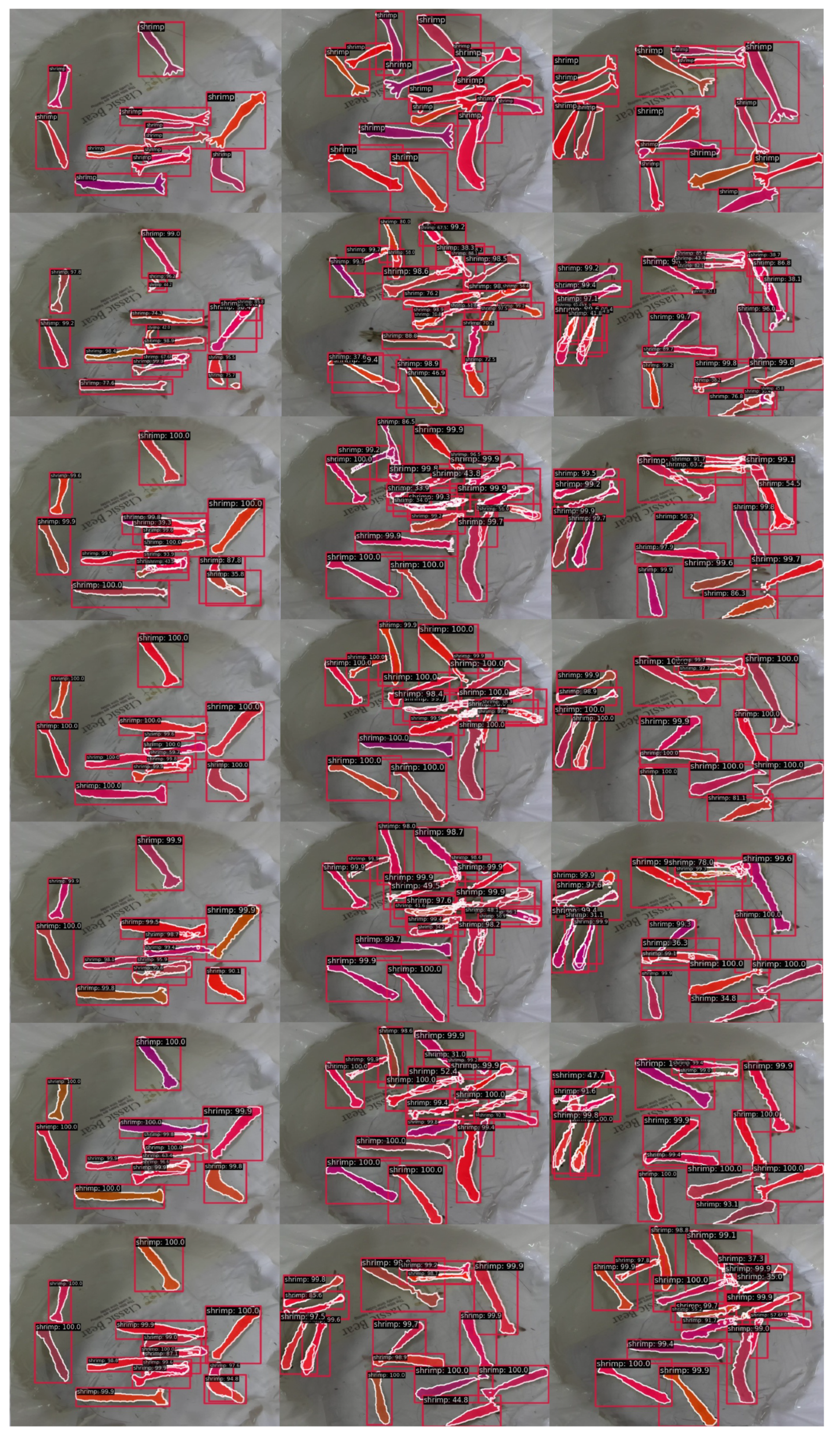
These experimental results strongly support our argument that combining the unsupervised learning method of contrastive learning for fine-tuning can achieve better experimental results than directly fine-tuning, even though the contrastive learning model is not pre-trained on the specific dataset. When training the contrastive learning model, it can learn potential feature representations in the dataset through contrastive loss, which can better segment the target. Several instance segmentation results are visualized in Figure 4, which clearly demonstrate that MoCov2 exhibits relatively better segmentation quality compared to the other methods.
4.4. Ablation Studies
4.4.1. Input Size Comparisons
The selection of data augmentations has a significant impact on the performance of contrastive learning models during training. Among the commonly used data augmentation methods, the random resized crop is one that is often employed. However, this data augmentation method can be affected by different input sizes. In the original papers on the five contrastive learning models, the dataset used was ImageNet [31], which has image sizes of . However, this image size is too small for our shrimp dataset, which has a resolution of . Using such a small image size would result in the loss of many important image details. Therefore, we trained the five contrastive learning models with both the ImageNet size and our shrimp dataset size. The first five sub-figures of Figure 3 show the visualization of the training loss for the two different input sizes. We observe that both input sizes result in the convergence of the models during training. The convergent values of the models are very similar under the two different input sizes, especially for Byol, SimCLR, and MoCov3, where the convergence values are almost the same. Therefore, we can assume that the different input sizes have little effect on the training of the contrastive learning model and can be ignored.
4.4.2. Data Scale Comparisons
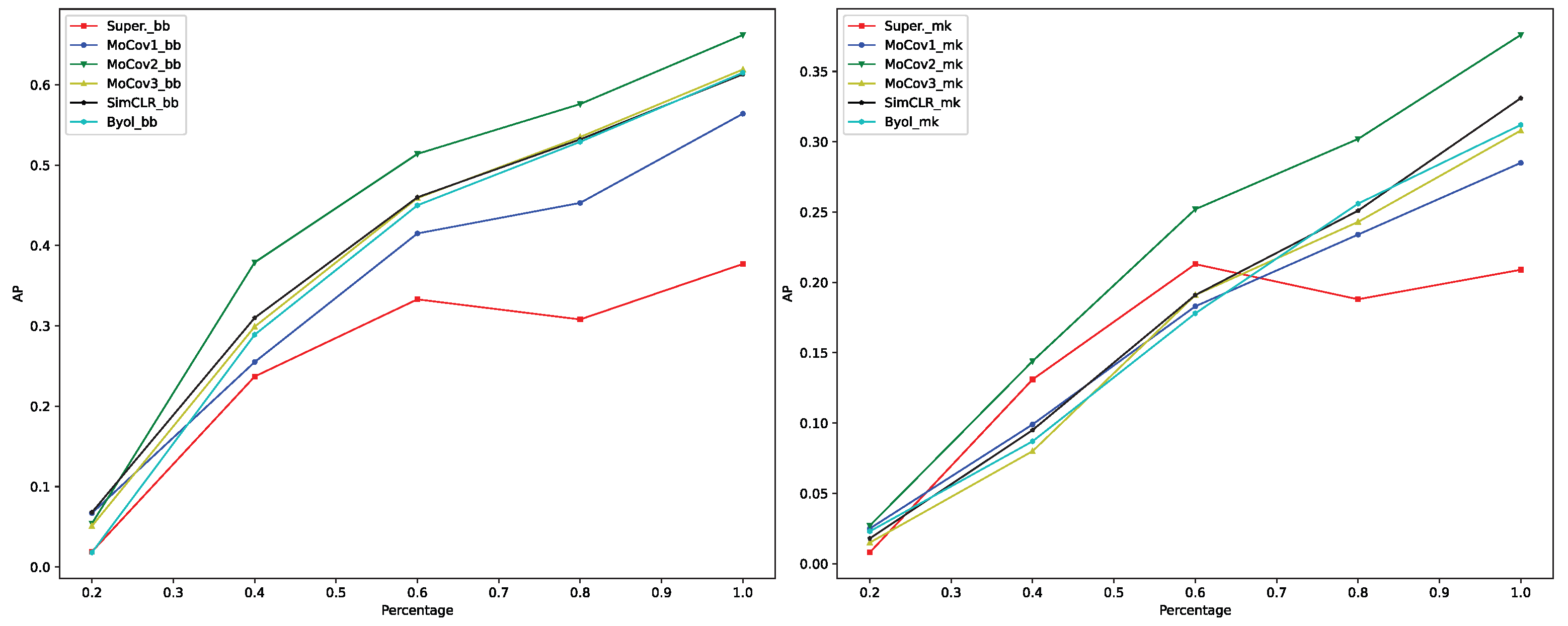
The use of a network trained with contrastive learning as the backbone of an instance segmentation network offers several advantages, including the ability to achieve a relatively high accuracy with a small labeled dataset. This is because the backbone trained with contrastive learning can efficiently extract features containing semantic information from images, allowing the subsequent modules in the instance segmentation network to obtain more precise features, which in turn ensures the accuracy of the pixel-wise classification and bounding box regression. Table 3 presents the instance segmentation results under different data scales, where the number of images in the training dataset is 800 and the number of images in the test dataset is 100 for all data scales. Figure 5 shows the visualized curves of the table. The results indicate that fine-tuning using contrastive learning models performs better than the common supervised learning method in terms of the bounding box regression task under all training data scales. MoCov2 achieves the best performance among all other methods when the training dataset is larger than 20%. When the training dataset is less than 60%, the supervised learning method can outperform the contrastive learning models in the mask segmentation task, except for MoCov2, and the difference is relatively small. When the amount of training data increases, the contrastive learning models perform better than the direct fine-tuning method, and the difference becomes more significant. These results effectively demonstrate the effectiveness of our idea that fine-tuning using contrastive learning models can outperform the commonly used fine-tuning method.
5. Conclusions
In this paper, we propose a novel approach to integrate state-of-the-art unsupervised learning with shrimp farming to reduce the reliance on labeled data in the instance segmentation of shrimp. We first build a shrimp dataset to facilitate the application of computer vision techniques in shrimp farming. This dataset contains two sub-datasets, where the first sub-dataset has about 10 k shrimp images without any label information, and can be used for training unsupervised learning models. The other one has 1 k shrimp images with high-quality label information. We then train five state-of-the-art contrastive learning models, including MoCov1, MoCov2, MoCov3, SimCLR, and Byol, and take them as a pre-trained backbone for fine-tuning the Mask R-CNN model. The experimental results show that compared with directly fine-tuning the full Mask R-CNN model, using a contrastive learning model as the backbone and then fine-tuning the rest of the modules in the Mask R-CNN model results in better performance, even though the contrastive learning model is not pre-trained on the shrimp dataset in advance. Furthermore, with the increase in data scale, the performance in terms of fine-tuning the Mask R-CNN model with a contrastive learning model as the backbone surpasses the common fine-tuning method with an increasing margin. In the comparisons of five contrastive learning models, MoCov2 outperforms other models in the instance segmentation task. These experimental results show the effectiveness of incorporating unsupervised learning with instance segmentation, which can lead to significant cost savings in shrimp farming. The approach proposed in this paper can also be extended to other fields of application with minimal modifications.
Author Contributions
Conceptualization, H.Z. and S.C.K.; methodology, H.Z.; data collection, S.H.K. and S.W.K.; supervision, S.C.K. and H.K.; writing, H.Z. and S.C.K.; visualization, H.Z.; funding acquisition, S.C.K., C.W.K. and H.K. All authors have read and agreed to the published version of the manuscript.
Funding
This research was supported by Korea Institute of Marine Science & Technology Promotion (KIMST) funded by the Ministry of Oceans and Fisheries (20210460).
Data Availability Statement
Acknowledgments
We express our greatest appreciation to Donghun Shin and Dongheon Seo for their help in labeling the data.
Conflicts of Interest
The authors declare no conflict of interest.
Abbreviations
The following abbreviations are used in this manuscript:
| CL | Contrastive Learning |
| MoCo | Momentum Contrast |
| MAP | Mean Average Precision |
| ViT | Vision Transformer |
| SGD | Stochastic Gradient Descent |
| AP | Average Precision |
| IoU | Intersection over Union |
| Average Precision at IoU 0.50 | |
| Average Precision at IoU 0.75 | |
| bb | Bounding Box |
| mk | Mask |
References
- Mahmud, H.; Rahaman, M.A.; Hazra, S.; Ahmed, S. IoT Based Integrated System to Monitor the Ideal Environment for Shrimp Cultivation with Android Mobile Application. Eur. J. Inf. Technol. Comput. Sci. 2023, 3, 22–27. [Google Scholar] [CrossRef]
- Armalivia, S.; Zainuddin, Z.; Achmad, A.; Wicaksono, M.A. Automatic Counting Shrimp Larvae Based You Only Look Once (YOLO). In Proceedings of the 2021 International Conference on Artificial Intelligence and Mechatronics Systems (AIMS), Bandung, Indonesia, 28–30 April 2021; IEEE: Piscataway, NJ, USA, 2021; pp. 1–4. [Google Scholar]
- Solahudin, M.; Slamet, W.; Dwi, A. Vaname (Litopenaeus vannamei) shrimp fry counting based on image processing method. Iop Conf. Ser. Earth Environ. Sci. 2018, 147, 012014. [Google Scholar] [CrossRef]
- Thai, T.T.N.; Nguyen, T.S.; Pham, V.C. Computer vision based estimation of shrimp population density and size. In Proceedings of the 2021 International symposium on electrical and electronics engineering (ISEE), Ho Chi Minh, Vietnam, 15–16 April 2021; IEEE: Piscataway, NJ, USA, 2021; pp. 145–148. [Google Scholar]
- Yu, H.; Liu, X.; Qin, H.; Yang, L.; Chen, Y. Automatic Detection of Peeled Shrimp Based on Image Enhancement and Convolutional Neural Networks. In Proceedings of the 8th International Conference on Computing and Artificial Intelligence, Tianjin, China, 18–21 March 2022; pp. 439–450. [Google Scholar]
- Zhang, L.; Zhou, X.; Li, B.; Zhang, H.; Duan, Q. Automatic shrimp counting method using local images and lightweight YOLOv4. Biosyst. Eng. 2022, 220, 39–54. [Google Scholar] [CrossRef]
- Hadsell, R.; Chopra, S.; LeCun, Y. Dimensionality reduction by learning an invariant mapping. In Proceedings of the 2006 IEEE Computer Society Conference on Computer Vision and Pattern Recognition (CVPR’06), New York, NY, USA, 17–22 June 2006; IEEE: Piscataway, NJ, USA, 2006; Volume 2, pp. 1735–1742. [Google Scholar]
- He, K.; Fan, H.; Wu, Y.; Xie, S.; Girshick, R. Momentum contrast for unsupervised visual representation learning. In Proceedings of the IEEE/CVF Conference on Computer Vision and Pattern Recognition, Seattle, WA, USA, 13–19 June 2020; pp. 9729–9738. [Google Scholar]
- Chen, X.; Fan, H.; Girshick, R.; He, K. Improved baselines with momentum contrastive learning. arXiv 2020, arXiv:2003.04297. [Google Scholar]
- Chen, X.; Xie, S.; He, K. An empirical study of training self-supervised vision transformers. In Proceedings of the IEEE/CVF International Conference on Computer Vision, Montreal, QC, Canada, 11–17 October 2021; pp. 9640–9649. [Google Scholar]
- Chen, T.; Kornblith, S.; Norouzi, M.; Hinton, G. A simple framework for contrastive learning of visual representations. In Proceedings of the International Conference on Machine Learning, Virtual, 13–18 July 2020; pp. 1597–1607. [Google Scholar]
- Grill, J.B.; Strub, F.; Altché, F.; Tallec, C.; Richemond, P.; Buchatskaya, E.; Doersch, C.; Avila Pires, B.; Guo, Z.; Gheshlaghi Azar, M.; et al. Bootstrap your own latent-a new approach to self-supervised learning. Adv. Neural Inf. Process. Syst. 2020, 33, 21271–21284. [Google Scholar]
- He, K.; Zhang, X.; Ren, S.; Sun, J. Deep residual learning for image recognition. In Proceedings of the IEEE Conference on Computer Vision and Pattern Recognition, Las Vegas, NV, USA, 27–30 June 2016; pp. 770–778. [Google Scholar]
- He, K.; Gkioxari, G.; Dollár, P.; Girshick, R. Mask r-cnn. In Proceedings of the IEEE International Conference on Computer Vision, Venice, Italy, 22–29 October 2017; pp. 2961–2969. [Google Scholar]
- Lin, T.Y.; Maire, M.; Belongie, S.; Hays, J.; Perona, P.; Ramanan, D.; Dollár, P.; Zitnick, C.L. Microsoft coco: Common objects in context. In Proceedings of the Computer Vision–ECCV 2014: 13th European Conference, Zurich, Switzerland, 6–12 September 2014; Proceedings, Part V 13. pp. 740–755. [Google Scholar]
- Redmon, J.; Divvala, S.; Girshick, R.; Farhadi, A. You only look once: Unified, real-time object detection. In Proceedings of the IEEE Conference on Computer Vision and Pattern Recognition, Las Vegas, NV, USA, 27–30 June 2016; pp. 779–788. [Google Scholar]
- Nguyen, K.T.; Nguyen, C.N.; Wang, C.Y.; Wang, J.C. Two-phase instance segmentation for whiteleg shrimp larvae counting. In Proceedings of the 2020 IEEE International Conference on Consumer Electronics (ICCE), Las Vegas, NV, USA, 4–6 January 2020; IEEE: Piscataway, NJ, USA, 2020; pp. 1–3. [Google Scholar]
- Bochkovskiy, A.; Wang, C.Y.; Liao, H.Y.M. Yolov4: Optimal speed and accuracy of object detection. arXiv 2020, arXiv:2004.10934. [Google Scholar]
- Howard, A.; Sandler, M.; Chu, G.; Chen, L.C.; Chen, B.; Tan, M.; Wang, W.; Zhu, Y.; Pang, R.; Vasudevan, V.; et al. Searching for mobilenetv3. In Proceedings of the IEEE/CVF International Conference on Computer Vision, Seoul, Republic of Korea, 27 October–2 November 2019; pp. 1314–1324. [Google Scholar]
- Hu, W.C.; Wu, H.T.; Zhang, Y.F.; Zhang, S.H.; Lo, C.H. Shrimp recognition using ShrimpNet based on convolutional neural network. J. Ambient. Intell. Humaniz. Comput. 2020, 1–8. [Google Scholar] [CrossRef]
- Liu, Z.; Jia, X.; Xu, X. Study of shrimp recognition methods using smart networks. Comput. Electron. Agric. 2019, 165, 104926. [Google Scholar] [CrossRef]
- Liu, Z. Soft-shell shrimp recognition based on an improved AlexNet for quality evaluations. J. Food Eng. 2020, 266, 109698. [Google Scholar] [CrossRef]
- Ronneberger, O.; Fischer, P.; Brox, T. U-net: Convolutional networks for biomedical image segmentation. In Proceedings of the Medical Image Computing and Computer-Assisted Intervention—MICCAI 2015: 18th International Conference, Munich, Germany, 5–9 October 2015; Proceedings, Part III 18. pp. 234–241. [Google Scholar]
- Yang, C.; An, Z.; Cai, L.; Xu, Y. Mutual contrastive learning for visual representation learning. Proc. Aaai Conf. Artif. Intell. 2022, 36, 3045–3053. [Google Scholar] [CrossRef]
- Ge, S.; Mishra, S.; Kornblith, S.; Li, C.L.; Jacobs, D. Hyperbolic Contrastive Learning for Visual Representations beyond Objects. arXiv 2022, arXiv:2212.00653. [Google Scholar]
- Wu, Y.; Wang, Z.; Zeng, D.; Li, M.; Shi, Y.; Hu, J. Decentralized unsupervised learning of visual representations. In Proceedings of the Proceedings of the Thirty-First, International Joint Conference on Artificial Intelligence, IJCAI, Vienna, Austria, 23–29 July 2022; pp. 2326–2333. [Google Scholar]
- Cole, E.; Yang, X.; Wilber, K.; Mac Aodha, O.; Belongie, S. When does contrastive visual representation learning work? In Proceedings of the IEEE/CVF Conference on Computer Vision and Pattern Recognition, New Orleans, LA, USA, 18–24 June 2022; pp. 14755–14764. [Google Scholar]
- Yu, E.; Li, Z.; Han, S. Towards Discriminative Representation: Multi-View Trajectory Contrastive Learning for Online Multi-Object Tracking. In Proceedings of the IEEE/CVF Conference on Computer Vision and Pattern Recognition (CVPR), New Orleans, LA, USA, 18–24 June 2022; pp. 8834–8843. [Google Scholar]
- Wang, P.; Han, K.; Wei, X.S.; Zhang, L.; Wang, L. Contrastive Learning Based Hybrid Networks for Long-Tailed Image Classification. In Proceedings of the IEEE/CVF Conference on Computer Vision and Pattern Recognition (CVPR), Nashville, TN, USA, 20–25 June 2021; pp. 943–952. [Google Scholar]
- Hou, S.; Shi, H.; Cao, X.; Zhang, X.; Jiao, L. Hyperspectral Imagery Classification Based on Contrastive Learning. IEEE Trans. Geosci. Remote Sens. 2022, 60, 1–13. [Google Scholar] [CrossRef]
- Deng, J.; Dong, W.; Socher, R.; Li, L.J.; Li, K.; Fei-Fei, L. Imagenet: A large-scale hierarchical image database. In Proceedings of the 2009 IEEE Conference on Computer Vision and Pattern Recognition, Miami, FL, USA, 20–25 June 2009; IEEE: Piscataway, NJ, USA, 2009; pp. 248–255. [Google Scholar]
- Dosovitskiy, A.; Beyer, L.; Kolesnikov, A.; Weissenborn, D.; Zhai, X.; Unterthiner, T.; Dehghani, M.; Minderer, M.; Heigold, G.; Gelly, S.; et al. An Image is Worth 16x16 Words: Transformers for Image Recognition at Scale. arXiv 2021, arXiv:2010.11929. [Google Scholar]
- Contributors, M. MMSelfSup: OpenMMLab Self-Supervised Learning Toolbox and Benchmark. 2021. Available online: https://github.com/open-mmlab/mmselfsup (accessed on 17 January 2023).
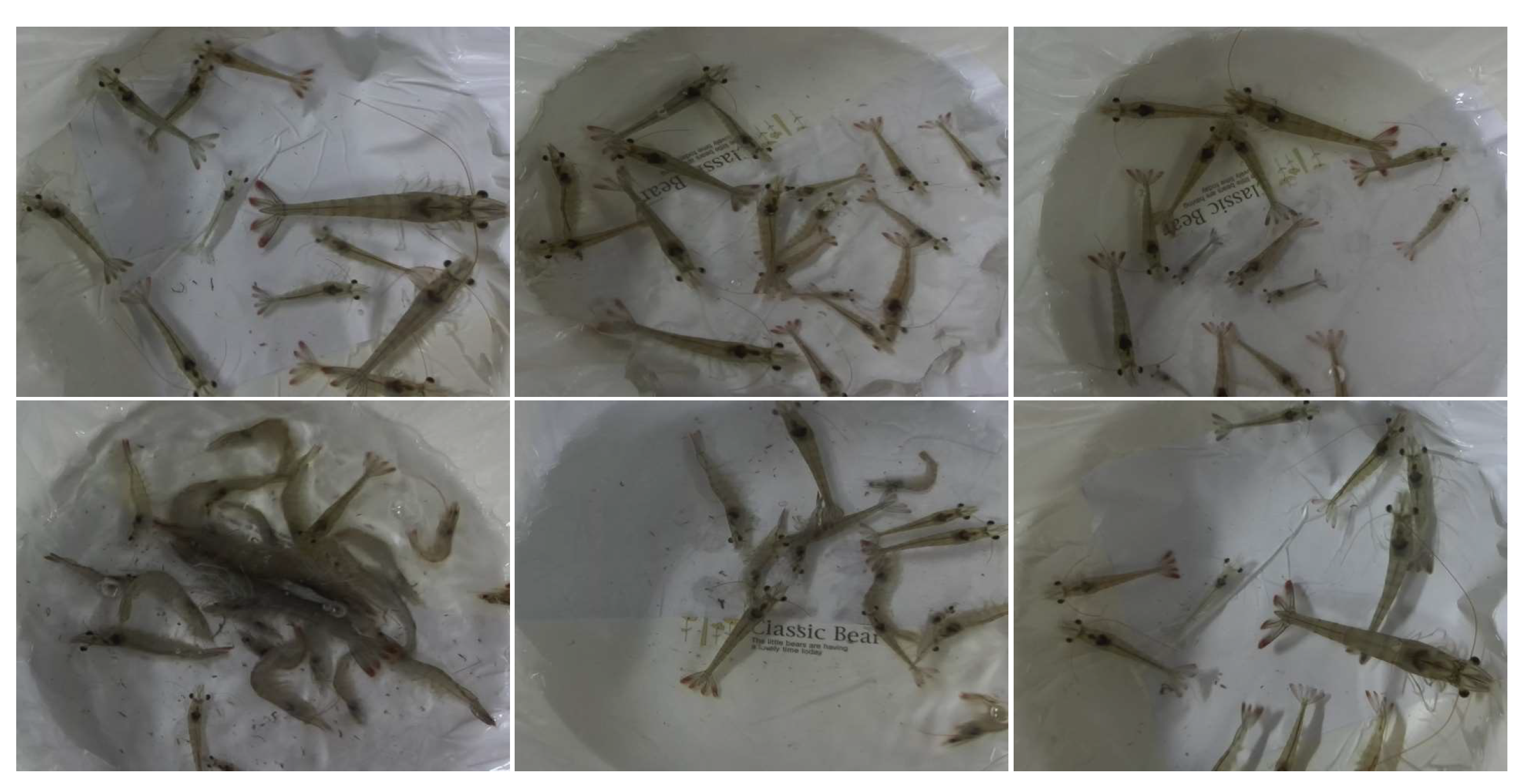
Figure 1.
Some examples of the shrimp images. There are five video sequences with different illumination, individual shrimp, shrimp density, and moving speed. This kind of setting provides much diversity to adapt to real-world application scenarios. The first five images come from the unlabeled dataset, from sequences one to five, respectively, and the last image is from the labeled dataset.

Figure 2.
The primary architecture proposed in this paper involves two main steps in training a network for the instance segmentation task. In the first step, a backbone for the Mask R-CNN is trained. We employ five contrastive learning strategies to train the backbones without labels and use them as pre-trained models. In the second step, the pre-trained models are fine-tuned with the Mask R-CNN. During fine-tuning, the parameters of the backbone are frozen, and only the parameters of the other part of the Mask R-CNN are updated.

Figure 3.
The visualization of the training loss from five contrastive learning models. The first five sub-figures are the loss comparison of two different input sizes of each model. The last sub-figure is the loss comparison of five models.
Figure 3.
The visualization of the training loss from five contrastive learning models. The first five sub-figures are the loss comparison of two different input sizes of each model. The last sub-figure is the loss comparison of five models.

Figure 4.
Some visualizations of instance segmentation. Each column represents one example. In each column, from top to bottom, we have the ground truth, the result of the supervised method, MoCov1, MoCov2, MoCov3, SimCLR, and Byol, respectively. (Image is better viewed when zoomed in).
Figure 4.
Some visualizations of instance segmentation. Each column represents one example. In each column, from top to bottom, we have the ground truth, the result of the supervised method, MoCov1, MoCov2, MoCov3, SimCLR, and Byol, respectively. (Image is better viewed when zoomed in).

Figure 5.
Average precision curves of the bounding box (left) and mask (right) under different data scales. and indicate the bounding box and mask, respectively.
Figure 5.
Average precision curves of the bounding box (left) and mask (right) under different data scales. and indicate the bounding box and mask, respectively.


Table 1.
The data augmentations used by each contrastive learning model.
| Models | Data Augmentations | ||
|---|---|---|---|
| MoCov1 [8] | RandomResizedCrop | RandomGrayscale | RandomFlip |
| MoCov2 [9] | RandomResizedCrop | RandomGrayscale | RandomFlip |
| RandomApply | RandomGaussianBlur | ||
| MoCov3 [10] | RandomResizedCrop | RandomGrayscale | RandomFlip |
| RandomApply | RandomGaussianBlur | RandomSolarize | |
| SimCLR [11] | RandomResizedCrop | RandomGrayscale | RandomFlip |
| RandomApply | RandomGaussianBlur | ||
| Byol [12] | RandomResizedCrop | RandomGrayscale | RandomFlip |
| RandomApply | RandomGaussianBlur | RandomSolarize | |
Table 2.
Instance segmentation results of using five contrastive learning models as the backbone for Mask R-CNN. and indicate the bounding box and mask, respectively. Random means the supervised fine-tuning method with the random initialization, and pre-trained denotes the supervised fine-tuning method using the weight file trained on a public dataset, such as the COCO dataset [15], as the initialization. MoCov2* is the contrastive learning model trained on the ImageNet [31] dataset.
| Super (random) | 0.228 | 0.657 | 0.08 | 0.08 | 0.393 | 0.002 |
| Super (pre-trained) | 0.377 | 0.743 | 0.352 | 0.209 | 0.645 | 0.045 |
| MoCov1 [8] | 0.564 | 0.916 | 0.579 | 0.285 | 0.761 | 0.107 |
| MoCov2 [9] | 0.662 | 0.945 | 0.739 | 0.376 | 0.84 | 0.24 |
| MoCov2* [9] | 0.684 | 0.955 | 0.786 | 0.363 | 0.837 | 0.226 |
| MoCov3 [10] | 0.619 | 0.941 | 0.684 | 0.308 | 0.798 | 0.12 |
| SimCLR [11] | 0.613 | 0.94 | 0.67 | 0.331 | 0.823 | 0.145 |
| Byol [12] | 0.615 | 0.941 | 0.672 | 0.312 | 0.804 | 0.128 |
Table 3.
Instance segmentation results of different training data scales. The numbers in the first row indicate the percentage of the whole training dataset, and the number of test images for all scales is the same, at 100 images.
Table 3.
Instance segmentation results of different training data scales. The numbers in the first row indicate the percentage of the whole training dataset, and the number of test images for all scales is the same, at 100 images.
| 20% | 40% | 60% | 80% | 100% | ||
|---|---|---|---|---|---|---|
| Super.(pre-trained) | 0.019 | 0.237 | 0.333 | 0.308 | 0.377 | |
| 0.008 | 0.131 | 0.213 | 0.188 | 0.209 | ||
| MoCov1 [8] | 0.067 | 0.255 | 0.415 | 0.453 | 0.564 | |
| 0.025 | 0.099 | 0.183 | 0.234 | 0.285 | ||
| MoCov2 [9] | 0.054 | 0.379 | 0.514 | 0.576 | 0.662 | |
| 0.027 | 0.144 | 0.252 | 0.302 | 0.376 | ||
| MoCov3 [10] | 0.051 | 0.299 | 0.459 | 0.535 | 0.619 | |
| 0.015 | 0.08 | 0.191 | 0.243 | 0.308 | ||
| SimCLR [11] | 0.068 | 0.31 | 0.46 | 0.532 | 0.613 | |
| 0.018 | 0.095 | 0.191 | 0.251 | 0.331 | ||
| Byol [12] | 0.018 | 0.289 | 0.45 | 0.529 | 0.615 | |
| 0.023 | 0.087 | 0.178 | 0.256 | 0.312 |
Disclaimer/Publisher’s Note: The statements, opinions and data contained in all publications are solely those of the individual author(s) and contributor(s) and not of MDPI and/or the editor(s). MDPI and/or the editor(s) disclaim responsibility for any injury to people or property resulting from any ideas, methods, instructions or products referred to in the content. |
© 2023 by the authors. Licensee MDPI, Basel, Switzerland. This article is an open access article distributed under the terms and conditions of the Creative Commons Attribution (CC BY) license (https://creativecommons.org/licenses/by/4.0/).
Share and Cite
MDPI and ACS Style
Zhou, H.; Kim, S.H.; Kim, S.C.; Kim, C.W.; Kang, S.W.; Kim, H. Instance Segmentation of Shrimp Based on Contrastive Learning. Appl. Sci. 2023, 13, 6979. https://doi.org/10.3390/app13126979
AMA Style
Zhou H, Kim SH, Kim SC, Kim CW, Kang SW, Kim H. Instance Segmentation of Shrimp Based on Contrastive Learning. Applied Sciences. 2023; 13(12):6979. https://doi.org/10.3390/app13126979
Chicago/Turabian StyleZhou, Heng, Sung Hoon Kim, Sang Cheol Kim, Cheol Won Kim, Seung Won Kang, and Hyongsuk Kim. 2023. "Instance Segmentation of Shrimp Based on Contrastive Learning" Applied Sciences 13, no. 12: 6979. https://doi.org/10.3390/app13126979
Note that from the first issue of 2016, this journal uses article numbers instead of page numbers. See further details here.