Article

Multiscale Applications of Two Online-Coupled Meteorology-Chemistry Models during Recent Field Campaigns in Australia, Part I: Model Description and WRF/Chem-ROMS Evaluation Using Surface and Satellite Data and Sensitivity to Spatial Grid Resolutions

1
Department of Marine, Earth and Atmospheric Sciences, North Carolina State University, Raleigh, NC 27695, USA
2
Centre for Atmospheric Chemistry, University of Wollongong, Wollongong, NSW 2500, Australia
3
School of Earth Sciences, University of Melbourne, Melbourne, Victoria, VIC 3052, Australia
4
Climate Science Centre, The Commonwealth Scientific and Industrial Research Organisation, Oceans and Atmosphere, Aspendale, VIC 3195, Australia
*
Author to whom correspondence should be addressed.
Atmosphere 2019, 10(4), 189; https://doi.org/10.3390/atmos10040189
Submission received: 26 February 2019 / Revised: 1 April 2019 / Accepted: 4 April 2019 / Published: 8 April 2019
(This article belongs to the Special Issue Air Quality in New South Wales, Australia)

Abstract

:
Air pollution and associated human exposure are important research areas in Greater Sydney, Australia. Several field campaigns were conducted to characterize the pollution sources and their impacts on ambient air quality including the Sydney Particle Study Stages 1 and 2 (SPS1 and SPS2), and the Measurements of Urban, Marine, and Biogenic Air (MUMBA). In this work, the Weather Research and Forecasting model with chemistry (WRF/Chem) and the coupled WRF/Chem with the Regional Ocean Model System (ROMS) (WRF/Chem-ROMS) are applied during these field campaigns to assess the models’ capability in reproducing atmospheric observations. The model simulations are performed over quadruple-nested domains at grid resolutions of 81-, 27-, 9-, and 3-km over Australia, an area in southeastern Australia, an area in New South Wales, and the Greater Sydney area, respectively. A comprehensive model evaluation is conducted using surface observations from these field campaigns, satellite retrievals, and other data. This paper evaluates the performance of WRF/Chem-ROMS and its sensitivity to spatial grid resolutions. The model generally performs well at 3-, 9-, and 27-km resolutions for sea-surface temperature and boundary layer meteorology in terms of performance statistics, seasonality, and daily variation. Moderate biases occur for temperature at 2-m and wind speed at 10-m in the mornings and evenings due to the inaccurate representation of the nocturnal boundary layer and surface heat fluxes. Larger underpredictions occur for total precipitation due to the limitations of the cloud microphysics scheme or cumulus parameterization. The model performs well at 3-, 9-, and 27-km resolutions for surface O3 in terms of statistics, spatial distributions, and diurnal and daily variations. The model underpredicts PM2.5 and PM10 during SPS1 and MUMBA but overpredicts PM2.5 and underpredicts PM10 during SPS2. These biases are attributed to inaccurate meteorology, precursor emissions, insufficient SO2 conversion to sulfate, inadequate dispersion at finer grid resolutions, and underprediction in secondary organic aerosol. The model gives moderate biases for net shortwave radiation and cloud condensation nuclei but large biases for other radiative and cloud variables. The performance of aerosol optical depth and latent/sensible heat flux varies for different simulation periods. Among all variables evaluated, wind speed at 10-m, precipitation, surface concentrations of CO, NO, NO2, SO2, O3, PM2.5, and PM10, aerosol optical depth, cloud optical thickness, cloud condensation nuclei, and column NO2 show moderate-to-strong sensitivity to spatial grid resolutions. The use of finer grid resolutions (3- or 9-km) can generally improve the performance for those variables. While the performance for most of these variables is consistent with that over the U.S. and East Asia, several differences along with future work are identified to pinpoint reasons for such differences.

1. Introduction

Despite significant improvement in urban air quality in Australia over the last decade, air pollution, and associated human exposure continue to attract research attention, especially in Greater Sydney area where more than 5 million people (about 21% of the total population in Australia) breathe poor quality air and experience decreased life expectancy [1]. The latest Australian State of the Environment report indicated increased adverse impact of air pollution on human health since 2011, and observed health effects at lower pollutant concentrations than those on which the guidelines are based [2]. Major sources of pollutants include anthropogenic emissions from industry, transportation, biomass burning, domestic wood heaters, and natural emissions of sea-salt and dust particles. Industrial and biogenic emissions (e.g., bushfires, dust storms) and extreme events (e.g., heat waves) are associated with the worst air pollution episodes [3,4,5,6,7,8,9,10,11,12,13,14,15]. For example, Duc et al. [15] conducted a source apportionment for surface ozone (O3) concentrations in the New South Wales Greater Metropolitan Region and found that biogenic volatile organic compound (VOC) emissions and anthropogenic emissions from commercial and domestic sources contribute significantly to high O3 concentration in North West Sydney during summer. Utembe et al. [16] also reported a key role that biogenic emissions from Eucalypts played in high O3 episodes during extreme heat periods in January 2013 in Greater Sydney. As a consequence of exposure to polluted air, more than 3000 premature deaths per year from air pollution occur in urban areas [17,18] where more than 70% Australians live [2,19]. The premature death associated with chronic exposure to PM2.5 in Sydney, Melbourne, Brisbane, and Perth is estimated to be 1586/year averaged over 2006–2010 [1]. In the Sydney metropolitan area, 430 premature deaths and 5800 years of life lost were attributable to 2007 levels of PM2.5 and ~630 respiratory and cardiovascular hospital admissions were attributable to 2007 PM2.5 and O3 exposures [20].
Three field campaigns were conducted in New South Wales (NSW) through a collaborative project among seven research organizations and universities in Australia to characterize the pollution sources and their impacts on ambient air quality and human exposure in support of air quality control policy-making by NSW Office of the Environment and Heritage (OEH) [21,22]. These include the Sydney Particle Study (SPS) Stages 1 and 2 in western Sydney during summer 2011 (5 February to 7 March) and Autumn 2012 (16 April to 14 May), respectively, and the Measurements of Urban, Marine, and Biogenic Air (MUMBA) campaign in Wollongong during summer 2013 (21 December–15 February 2013) [23,24]. Comprehensive measurements of trace gases, aerosol, and meteorological variables were made during these field campaigns. During SPS1, the meteorological conditions were not significantly different from the long-term average for the Sydney region. The weather was driven by high pressure systems. North-westerly winds are prevalent, most days are dry except for February 6, 2011 during which heavy rain occurred in the south of NSW [25]. During SPS2, warmer than average temperatures occurred across the Sydney region. The weather was driven by low pressure systems, leading to lower solar insolation and ventilation rates, and calmer conditions with weaker mixing of the atmosphere than SPS1. The low pressure systems also brought heavy precipitation during April 17–19, 2012. During MUMBA, anticyclone was the dominant circulation pattern [26]. It covered the hottest summer on record for Australia with two extremely hot days with maximum temperatures above 40 °C in the Greater Sydney region: January 8 and January 18, 2013 [16,27,28], leading to very different conditions from a typical summer in this region. The record-high rainfall in January occurred during January 28–29 in this region. Increased boundary layer height and strong sea breezes were observed in this region [23]. Different meteorological conditions during these field campaigns caused different concentrations of air pollutants. For example, the observed concentrations of CO, NO2, toluene, and xylenes at the Westmead Observatory were higher by 1.5–3 times during SPS1 than SPS2 [22]. The observed O3, PM2.5, and PM10 concentrations in this region during MUMBA are higher than those of SPS1. These field campaigns therefore provide useful contrasting testbeds to evaluate model performance under various meteorological and chemical conditions.
Increasing numbers of 3D chemical transport models have been applied to simulate air quality in Australia and its subareas in recent years. As part of SPS1 and SPS2, a chemical transport model, i.e., the CSIRO Chemistry Transport Model (CSIRO-CTM) [29] was applied to simulate air quality during SPS1 and SPS2 [21,22]. CSIRO-CTM is a 3-D offline model that is driven by meteorological fields pre-generated using a 3-D numerical weather model. As part of the Clean Air and Urban Landscapes (CAUL) regional air quality modeling project, six regional models were applied over the three field campaign periods to simulate air quality and understand the sources of air pollution. These models include CSIRO-CTM, an operational version of CSIRO-CTM operated by the New South Wales Office of Environment and Heritage (NSW OEH), offline-coupled Weather Research and Forecasting model v3.6.1-Community Multiscale Air Quality modeling system (WRF-CMAQ), two versions of the WRF model with chemistry (WRF/Chem) v3.7.1 with different chemical mechanisms and physical options applied by the University of Melbourne and North Carolina State University (WRF/Chem-UM and WRF/Chem-NCSU, respectively), and the coupled WRF/Chem v3.7.1 with the Regional Ocean Model System (ROMS) (WRF/Chem-ROMS). Observational data from these field campaigns were used to validate the model performance. More detailed descriptions of the intercomparison of meteorological and air quality predictions by the six models can be found in Monk et al. [28] and Guerette et al. [30]. Model application and evaluation for SPS1 and SPS2 using the modified CSIRO-CTM and for MUMBA using WRF/Chem-UM can be found in Chang et al. [31] and Utembe et al. [16], respectively.
In this work, as part of the CAUL model intercomparison project, two advanced online-coupled meteorology-chemistry models, WRF/Chem, and WRF/Chem-ROMS are applied during these field campaign periods. WRF/Chem has been mostly applied over the Northern Hemisphere (NH) including North America, Europe, and Asia [32,33,34,35,36,37,38]. There are only limited numbers of applications over the Southern Hemisphere (SH) (e.g., [16,39]), in particular over Australia. WRF/Chem-ROMS has been recently applied to the U.S. [40]. It has not been applied to other regions in the world. The overarching objectives of this work are to evaluate the predictions from the two models using surface observations from these field campaigns and satellite retrievals and identify likely causes for model biases and areas of improvements for their applications in the SH with distinct characteristics of meteorology, emissions, and chemistry from the NH where the two models were originally developed and mostly evaluated. The results are presented in two papers. The first paper describes the models, configurations, evaluation protocols, as well as the WRF/Chem-ROMS model evaluation results using available field campaign data and satellite retrievals. The sensitivity of the model predictions to spatial grid resolutions is also evaluated. The second paper intercompares results from WRF/Chem with those from WRF/Chem-ROMS and investigate the impacts of air–sea interaction and boundary conditions on radiative meteorological, and chemical predictions.

2. Model Setup and Evaluation Protocols

2.1. Model Description

The Weather Research and Forecasting model with Chemistry (WRF/Chem) was originally co-developed by U.S. National Center for Atmospheric Research and National Oceanic and Atmospheric Administration and further developed by scientific communities [32]. WRF/Chem v3.7.1 =by the North Carolina State University (NCSU) (WRF/Chem-NCSU) is based on the NCSU’s version of WRF/Chem v3.7.1 [41,42]. WRF/Chem v3.7.1-ROMS is based on the NCSU’s version of WRF/Chem v3.7.1 coupled with the Regional Ocean Modeling System (ROMS) (WRF/Chem-ROMS) [40]. WRF/Chem-ROMS was developed by NCSU based on coupled WRF-ROMS within the Coupled Ocean-Atmosphere-Wave-Sediment Transport (COAWST) Modeling System [43]. ROMS is a 3-D, free-surface, hydrostatic, and primitive equations ocean model [44]. It simulates advective processes, Coriolis, and viscosity and includes the high-order advection and time-stepping schemes, weighted temporal averaging of the barotropic mode, conservative parabolic splines for vertical discretization, and the barotropic pressure gradient term, which can be applied for estuarine, coastal, and basin-scale oceanic processes [45,46,47]. The coupling of WRF/Chem and ROMS within WRF/Chem-ROMS enable dynamic interactions between atmosphere and ocean, with net heat flux and wind stress information passing from WRF to ROMS and the calculated SST passing from ROMS to WRF.
The physics options selected for the WRF/Chem simulations include the Rapid and accurate Radiative Transfer Model for GCM (RRTMG) [48] for both shortwave and longwave radiation, the Yonsei University (YSU) planetary boundary layer (PBL) scheme [49,50], the single layer urban canopy model, the National Center for Environmental Prediction, Oregon State University, Air Force, and Hydrologic Research Lab (NOAH) [51,52], the Morrison et al. [53] double moment microphysics scheme (M09), as well as the Multi-Scale Kain–Fritsch (MSKF) cumulus parameterization [54]. The gas-phase chemistry is simulated using the Carbon Bond 2005 (CB05) gas mechanism of Yarwood et al. [55] with the chlorine chemistry of Sarwar et al. [56]. The aerosol model selected is the Modal for Aerosol Dynamics in Europe/Volatility Basis Set (MADE/VBS) aerosol module of Ahmadov et al. [57]. CB05 was coupled with MADE/VBS within WRF/Chem by Wang et al. [48] and this chemistry/aerosol option allows the simulations of aerosol direct, semi-direct, and indirect effect. Aqueous-phase chemistry is simulated for both resolved and convective clouds using the AQ chemistry module (AQCHEM) that is similar to the AQCHEM module in CMAQv4.7 of Sarwar et al. [58]. The aerosol activation parameterization is based on the Abdul-Razzak and Ghan scheme [59,60].
The aerosol direct and indirect effect treatments in WRF/Chem are similar to those described in Chapman et al. [61] but with updated schemes for radiation and cloud microphysics schemes. Aerosol radiative properties are simulated based on the Mie theory. Aerosol direct radiative forcing is calculated using the RRTMG. The aerosol indirect effects are simulated through aerosol-cloud-radiation-precipitation interactions. The Cloud Condensation Nuclei (CCN) spectrum is determined based on the Köhler theory as a function of aerosol number concentrations and updraft velocity following the aerosol activation/resuspension parameterization of Abdul-Razzak and Ghan [60]. The subgrid updraft velocity is calculated from turbulence kinetic energy for all layers above surface and diagnosed from eddy diffusivity. The same parameterization was used to calculate updraft velocities on different nested domains. Cloud droplet number concentrations (CDNC) are simulated by accounting for their changes due to major cloud processes including droplet nucleation/aerosol activation, advection, collision/coalescence, collection by rain, ice, and snow, and freezing to form ice crystals following the parameterization of Ghan et al. [62], which has been added to the existing M09 microphysics scheme to allow the two-moment treatment of cloud water. The cloud-precipitation interactions are simulated by accounting for the dependence of autoconversion of cloud droplets to rain droplets on CDNC based on the parameterization of Liu et al. [63]. The cloud-radiation interactions are simulated by linking simulated CDNC with the RRTMG and the M09 microphysics scheme. Although the cloud treatments in the M09 scheme remain parameterized and they are based on the two-moment modal cloud size distribution, they are much more physically-based, as compared to most models that use highly-simplified cloud microphysics and diagnose CDNC.
The WRF/Chem-ROMS simulation uses the same physics and chemistry options as WRF/Chem except that it explicitly simulates air–sea interactions and the sea surface temperature (SST). Similar to nearly all past WRF/Chem applications [32,33,34,35,36,37,38,39,64,65,66,67,68,69], the SST is prescribed using NCEP high-res SST analysis (RTG_SST) data [70,71] for the WRF/Chem simulation but simulated by ROMS for the WRF/Chem-ROMS simulation. As shown in He et al. [40], by explicitly simulating air–sea interactions and SST, WRF/Chem-ROMS can improve the predictions of most cloud and radiative variables compared to WRF/Chem that does not simulate such interactions.

2.2. Model Configurations

The model simulations using WRF/Chem and WRF/Chem-ROMS are performed over quadruple-nested domains at grid resolutions of 81-, 27-, 9-, and 3-km over Australia (d01), an area in southeastern Australia (d02), an area in New South Wales (NSW) (d03), and the Greater Sydney area (d04), respectively. The vertical resolution includes 34 layers from surface (~35 m) to approximately 100 hPa (~15 km). Figure 1 shows the simulation domains. Simulation periods for the three field campaigns over d01 are Jan 26–Mar 9, 2011, Apr 1–May 20, 2012, and Dec. 11, 2012–Feb. 20, 2013 for SPS1, SPS2, and MUMBA, respectively, with 10 days for spin-up. The analysis time periods are Feb. 5–Mar. 7, 2011 (Summer) for SPS1, Apr. 11–May 13, 2012 (Autumn) for SPS2, and Dec. 21–Feb. 15, 2013 (Summer) for MUMBA. Gridded analysis nudging of temperature, wind speed, water vapor with a nudging coefficient of 1 × 10⁻⁴ is applied above the PBL for both model simulations. For WRF/Chem-ROMS simulation, the time step for ROMS calculation is 30 s and the time frequency for the WRF/Chem-ROMS coupling is 10 min.
Anthropogenic emissions are based on EDGER-HTAP at 0.1° over Australia and the 2008 inventory from NSW-EPA at 1 × 1 km2 for inner domains covering the NSW Greater Metropolitan Region [72]. While the 2012/2013 Australia’s National Pollution Inventory is available, the NSW- EPA provides a more detailed inventory for the NSW greater metropolitan region, which is used in this work. Large uncertainties exist in both inventories with some large differences in the emissions over the NSW region [24]. For example, compared to the 2012/2013 NPI emission inventories, the 2008 NSW-EPA inventory gives the same NOx emissions, higher emissions of SO2, VOCs, and PM2.5 (by 29%, 55%, 601%, respectively) but lower emissions of CO and PM10 (by 11.7% and 34.5%, respectively) over the NSW region [24] during the MUMBA period. Biogenic emissions are calculated online using the Model of Emissions of Gases and Aerosols from Nature version 2 [73]. Dust emissions are calculated online with Atmospheric and Environmental Research Inc. and Air Force Weather Agency (AER/AFWA) schemes [74]. Emissions from sea salt are generated based on the scheme of Gong et al. [75]. The meteorological initial and boundary conditions for the outermost domain (i.e., d01) are based on the National Center for Environmental Prediction Final Analysis (NCEP-FNL). The chemical initial and boundary conditions for the simulation over d01 are based on the results from a global Earth system model, the NCSU’s version of the Community Earth System Model (CESM_NCSU) v1.2.2. For simulations over d02, d03, and d04, their initial and boundary conditions are based on the results from the simulations over d01, d02, and d03, respectively, and no spin-up was used. All simulations over d01-d04 are continuous simulations without restart. As described in several papers [76,77,78], CESM_NCSU includes similar representations of gas-phase chemistry, aerosol, and aerosol–cloud interactions to those used in WRF/Chem and WRF/Chem-ROMS, therefore effectively minimizing the uncertainties introduced by different model representations of key processes in the global and regional models. To further increase the accuracy of the chemical boundary conditions, the boundary conditions of CO, NO2, HCHO, O3, and PM species are constrained based on satellite observations of column abundance of CO, NO2, HCHO, and O3, as well as AOD (a proxy for PM column concentrations), respectively (see the Part II paper for more details). For ROMS, the initial and boundary conditions are from the global HYbrid Coordinate Ocean Model (HYCOM) combined with the Navy Coupled Ocean Data Assimilation (NCODA) (http://tds.hycom.org/thredds/catalog.html).

2.3. Evaluation Datasets and Protocols

Figure 2 shows the meteorological and air quality monitoring sites during the three field campaigns. Meteorological measurements are available at eight sites maintained by the Bureau of Meteorology (BoM). They are also available at 18 sites maintained by the NSW Office of Environment & Heritage (OEH), however, those sites are generally not ideal sites for meteorological measurements, thus, not included in the evaluation. Air quality measurements are available at 18 OEH sites. The performance statistics are calculated at all 18 sites for chemical predictions and at 8 BoM sites for meteorological performance. Site-specific analysis is performed at five BoM sites (i.e., Badgery’s Creek, Bankstown Airport, Bellambi, Richmond RAAF, and Sydney Airport) for meteorology and nine selected OEH sites (i.e., Bargo, Chullora, Earlwood, Bringelly, Liverpool, Oakdale, Randwick, Richmond, and Wollongong) for chemical concentrations. These sites represent various geographical locations within the greater Sydney area with different characteristics in emissions, meteorology, and topography. Seven-out-of-the-nine OEH sites are considered to be co-located with at least one BoM site, being within a distance of 15 km. For example, Earlwood is within 10 km and 15 km of Sydney Airport and Bankstown Airport, respectively, Liverpool and Chullora are within 9 km and 11 km of Bankstown Airport, respectively, Richmond is within 3.7 km of Richmond RAAF, Bringelly is within 9 km of Badgery’s Creek, Randwick is within 15 km of Sydney Airport, and Wollongong is within 9 km of Bellambi. The meteorological variables evaluated include 2-m temperature (T2), 2-m relative humidity (RH2), 10-m wind speed (WS10), wind direction (WD10), and precipitation against the BoM measurements. Additional precipitation data from satellite and reanalysis datasets are also used, including the Multi-Source Weighted-Ensemble Precipitation (MSWEP) [79] and the Global Precipitation Climatology Project (GPCP) (http://www.esrl.noaa.gov/psd/data/gridded/data.gpcp.html). MSWEP consists of global precipitation data with a 3-hour temporal resolution and a 0.25° spatial resolution, the daily data are used for the evaluation. GPCP consists of monthly global precipitation data at a 2.5° spatial resolution. The surface criteria pollutants evaluated include hourly concentrations of O3, CO, NO, NO2, SO2, PM2.5, and PM10. The column variables evaluated include the column abundance of carbon monoxide (CO) against Measurements of Pollution in the Troposphere (MOPITT), column nitrogen dioxide (NO2) and formaldehyde (HCHO) from the Global Ozone Monitoring Experiment (GOME), tropospheric ozone residual (TOR) from the Ozone Monitoring Experiment (OMI), aerosol optical depth (AOD), cloud condensation nuclei (CCN), cloud fraction (CF), cloud optical thickness (COT), cloud liquid water path (CWP), and precipitating water vapor (PWV) from the Moderate Resolution Imaging Spectroradiometer (MODIS), as well as net shortwave radiation (GSW), downward longwave radiation (GLW), and shortwave and longwave cloud forcing (SWCF and LWCF) against the Clouds and the Earth’s Radiant Energy System (CERES). Cloud droplet number concentration (CDNC) was derived by Bennartz [80] from MODIS. SST, latent heat flux (LHF), and sensible heat flux (SHF) prescribed by WRF/Chem and simulated by WRF/Chem-ROMS are also evaluated against the Objectively Analyzed Air–sea Fluxes (OAFlux) [81], which combines satellite data with modeling and reanalysis data (http://oaflux.whoi.edu/dataproducts.html). The OAFlux products are determined by using the best-possible estimates of flux-related surface meteorology and the state-of-the-science bulk flux parameterizations.
Emery and Tai [82] and Tesche et al. [83] proposed a set of statistical measures for benchmarks including root mean square error (RSME), mean gross error, mean bias (MB), and Index of Agreement (IOA) for T2, specific humidity, WS10, and WD10. For example, the recommended benchmark MBs for T2, WS10, and WD10 are ≤ ±0.5 °C, ≤ ±0.5 m s−1, and ≤ ±10°, respectively, which will be used in this work. Precipitation is one of the most difficult variables to be accurately predicted by mesoscale meteorological models, as it largely relies on the model representations of cloud microphysics, convection, and aerosol indirect effects, all of which contain large uncertainties. No published benchmarks are available to judge the model’s performance for precipitation. Based on previous applications of MM5 and WRF over various regions [36,37,40,66,67,84,85,86,87,88,89], NMBs within 30% represent the precipitation performance by current models, which will be used as a benchmark for precipitation in this work. For chemical concentrations, Zhang et al. [90] suggested good performance benchmarks of NMBs and NMEs within ±15% and 30% for O3 and PM2.5. However, while nearly all reported O3 performance met these criteria, most reported PM2.5 performance did not, indicating that accurately simulating PM2.5 is more challenging than O3, due to the complexity of the PM2.5 sources, chemistry and formation pathways, and removal processes, as well as its broad size range. Built on a comprehensive survey of criteria used in literature [33,34,35,90,91,92,93,94], Emery et al. [95] recommended criteria of NMB and NME of < ±15% and < 25% for O3 and < ±30% and < 50% for PM2.5, which will be used in this work.
The model evaluation includes the calculation of performance statistics and comparison of simulations and observations in terms of spatial distributions of predictions overlaid with observations and temporal variation. The performance statistics used for model evaluation include mean bias (MB), correlation coefficients (Corr), normalized mean bias (NMB), and normalized mean error (NME). The definitions of the statistical metrics can be found in Yu et al. [91] and Zhang et al. [85]. The domain-mean statistics are calculated for major meteorological and chemical variables based on paired averaged observation and simulation data during the same hours at all sites within each of the four domains for each field campaign. Since the satellite-derived data are available on a monthly basis, satellites retrievals in Feb. 2011, average of Apr. and May, 2012, and average of Jan. and Feb., 2013 are used to evaluate averaged predictions over SPS1, SPS2, and MUMBA, respectively. The satellite-derived data are regridded to the same domain for each grid cell.

3. Model Evaluation

3.1. Boundary Layer Meteorological Evaluation

Table 1, Table 2 and Table 3 summarize the performance statistics of meteorological and chemical predictions from WRF/Chem-ROMS during SPS1, SPS2, and MUMBA, respectively. For T2, the model is able to capture the seasonal variation with higher average temperatures in summer during SPS1 and MUMBA than those in autumn during SPS2, and higher T2 during MUMBA due to the heatwaves than SPS1. The domain-mean MBs of T2 during all field campaigns are in the range of −0.22 to 0.1°C at 27-, 9-, and 3-km resolutions but −0.9 to −0.5°C at 81-km resolution, indicating a satisfactory performance of T2 predictions except at 81-km. The model has the best statistical performance for T2 at 3-km for SPS2 and at 9-km for SPS1 and MUMBA. Over the ocean, SST is slightly overpredicted for SPS1, underpredicted for SPS2, and either overpredicted or underpredicted for MUMBA at all grid resolutions. The domain-mean MBs of SST are −1.7 to 1.4 °C at 81-km resolution and −0.5 to 1.0 °C at finer resolutions. For RH2, MBs are within 5%, NMBs are within 7%, and NMEs are within 15%, also indicating a good performance, although the model did not reproduce the observed relatively higher RH2 value during SPS2 than during SPS1 and MUMBA at all grid resolutions except at 81-km. For WS10, the model effectively simulates the seasonal variation with the strongest wind during MUMBA and the weakest wind during SPS2. The WS10 biases at 3-km are −0.09, 0.16, and −0.32 m s−1 for SPS1, SPS2, and MUMBA, the corresponding MBs for WD10 are within 9.5°, 1.9°, and 10.9°, respectively, which are within the performance threshold of 10° except for MUMBA. An overall good performance of WS10 and WD10 is also found at 9-km. In addition to accurate simulation of atmospheric stability and the use of a fine grid resolution, an accurate representation of surface roughness is required for accurate simulation of WS10. WRF has a tendency to overpredict WS10 because it cannot accurately resolve topography [96,97]. In this work, the good performance of WS10 at 3- and 9-km is because of the use of fine grid resolution and of the surface roughness correlation algorithm of Mass and Ovens [96]. However, the model shows relatively large biases for WS10 and WD10 at coarser grid resolutions (27- and 81-km) for SPS1 and SPS2, with their MBs ranging from −0.8 to 0.6 m s−1 and from −1.6° to 11.5 °, respectively, some of them exceed the performance threshold of 0.5 m s−1 for WS10 and 10° for WD10. This indicates a need to improve the model’s representation of subgrid scale variation of the topography, in particular surface roughness in Australia at coarse grid resolutions.
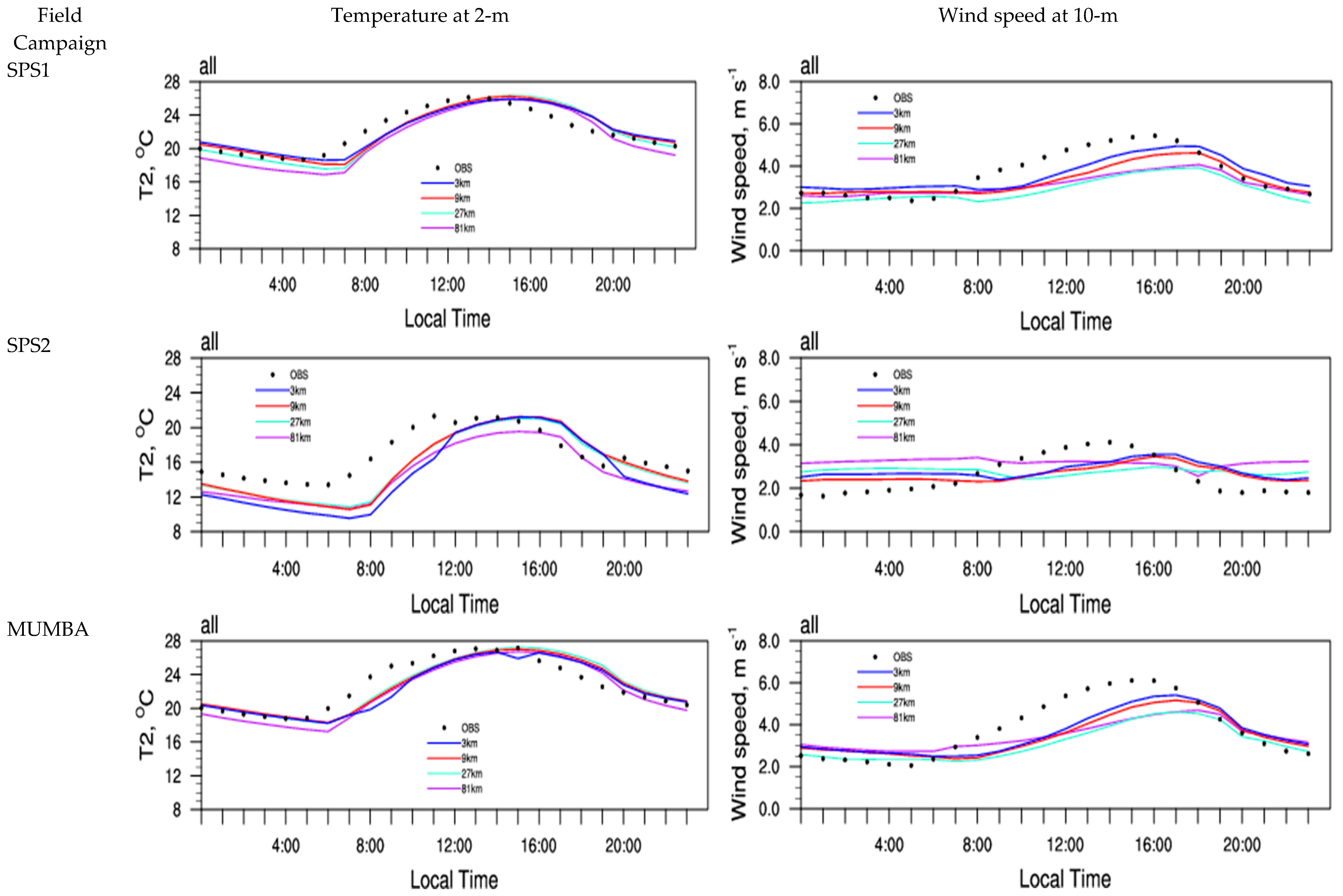
Figure 3 compares observed and simulated domain-mean diurnal profiles of T2 and WS10 averaged over all BoM monitoring stations over the Greater Sydney (d04) simulated by WRF/Chem-ROMS during SPS1, SPS2, and MUMBA. As expected, the predictions at 81-km deviate most significantly from the observations during most hours for both T2 and WS10 during all three field campaigns, whereas those at finer resolutions agree generally better with observations. The large deviation at 81-km is caused by the use of a coarse grid resolution that cannot accurately resolve heterogeneity of topography and small-scale meteorological processes and variables. The T2 predictions at 27-, 9-, and 3-km are similar, but WS10 predictions differ appreciably with better agreement at 9- and 3-km than at 27-km. For T2, the model tends to underpredict between 6 a.m. to noontime but overpredict after 2 p.m. For WS10, the model tends to overpredict before 8 a.m. and after late afternoon but underpredicted during the daytime. These deviations indicate the model’s difficulties in reproducing both daytime and nighttime profiles of T2 and WS10 in Australia, due to the limitations of the YSU PBL scheme and the NOAH land surface module in representing daytime and nocturnal boundary layer and surface sensible and latent heat fluxes over land areas. For example, the limitations in the nocturnal boundary layer representation may include inaccurate eddy diffusivities and nighttime mixing, and the strength and depth of the low-level jets [50,98,99,100].
Figure S1 in the supplementary material compares observed and simulated temporal profiles of T2 at five selected sites. During SPS1, SPS2, and MUMBA, T2 predictions at all grid resolutions are very similar at two inland sites (Badgery’s Creek and Richmond), but show higher sensitivity to horizontal grid resolutions at Bankstown Airport (an inland site), and Bellambi and Sydney Airport (coastal or near coastal sites), with better performance at 3-, 9-, and 27-km except at Bellambi during SPS1. During SPS1, the closest agreement with observations occurs for the simulation at 3-km at Bellambi and Bankstown Airport but for the simulation at 9-km at Sydney Airport. During SPS2, the closest agreement with observations occurs for the simulation at 9-km at Bankstown Airport but for the simulation at 27-km at Sydney Airport. During MUMBA, the closest agreement with observations occurs for the simulation at 9-km at Bankstown Airport and Sydney Airport. Comparison of temperature profiles during the three field campaigns shows strong observed seasonal variations with higher temperature in summer 2011 and 2013 (SPS1 and MUMBA) than in autumn (SPS2) at the same site (except at Bellambi where the observations are only available in summer 2012), which is reproduced well at all sites. The model also reproduces well the observed heat waves on Jan. 8 and Jan. 18, 2013 with higher daily maximum T2 values and a much stronger observed daily variation of T2 during summer 2013 than during summer 2011.
Figure S2 compares observed and simulated temporal profiles of WS10 at the same five sites. Compared to T2, WS10 predictions are much more sensitive to horizontal grid resolutions at all sites, generally with better performance at 3- and 9-km at most sites. During SPS1, WS10 predictions show the largest difference at Bellambi among the simulations with different grid resolutions, with the best performance at 3-km. Bellambi is very close to the ocean, a grid cell of 3 × 3 km2 most accurately represents the land surface at this site, whereas larger grid cells consist of some oceanic areas, leading to underpredictions of WS10. The best agreement with observation occurs at the Sydney Airport for the simulation at 3- and 9-km but at Badgery’s Creek, Bankstown Airport, and Richmond RAAF for the simulation at 27-km. The model tends to underpredict WS10 at the Sydney Airport, in addition to Bellambi. During SPS2, the WS10 predictions at 3- and 9-km are very close at all sites except Bellambi where the four sets of predictions are quite different (although no observations are available for performance evaluation). The best agreement with observation occurs at the Sydney Airport for the simulation at 3-km but at Badgery’s Creek, Bankstown Airport, and Richmond RAAF for the simulation at 9-km. The model tends to underpredict WS10 at the Sydney Airport but overpredict at other sites. During MUMBA, WS10 predictions from the four sets of simulations are very close at Bankstown Airport and Richmond RAAF, with an overall very good performance against observations. Simulated WS10 at 3-, 9-, and 27-km at Badgery’s Creek agree well with observations but are significantly overpredicted at 81-km. WS10 predictions are largely underpredicted at the Sydney Airport, with the best performance at 3-km. Similar to SPS1 and SPS2, the model tends to underpredict WS10 at the Sydney Airport. Observed WS10 are generally lower during autumn than during summer at all sites, which is not well reproduced because of overpredictions at all sites except at the Sydney Airport. As mentioned previously, the larger wind bias during SPS2 may be driven by less organized flow patterns in autumn compared to summer, in addition to the inaccurate representation of the surface roughness.
Precipitation predictions are evaluated using three sets of data, including the observations from the field campaign (OBS), satellite retrievals, and combined satellite data and reanalysis data from MSWEP and GPCP. Comparing to OBS, the domain-mean NMBs at all grid resolutions are generally within ±30% for SPS1 and SPS2 but in the range of -40.7% to -32.4%% for MUMBA, indicating a satisfactory or marginal performance against OBS during SPS1 and SPS2 but unsatisfactory performance during MUMBA. MUMBA is an atypical summer in terms of both temperature and precipitation. The observed daily average precipitation during MUMBA is much higher (by a factor of 6) than that during SPS1 which is dry. SPS2 is also wet with much higher total precipitation (by a factor of 5.3) than SPS1. The model performs reasonably well for precipitation against OBS over d04 in the dry period (SPS1) but moderately underpredicts precipitation in the wet periods (SPS2 and MUMBA). Comparing to MSWEP, the domain-mean NMBs at 81-, 27-, 9-, and 3-km are mostly beyond ±30%, indicating an unsatisfactory performance at all grid resolutions during all field campaigns except for 81- and 3-km during SPS1 and 81-km and 27-km during SPS2. Comparing to GPCP, the domain-mean NMBs at all grid resolutions are well within ±30% for SPS2, but beyond ±30% for SPS1 and MUMBA, indicating a satisfactory performance during SPS2 but an unsatisfactory performance during SPS1 and MUMBA. The model’s skills in predicting precipitation are not self-consistent because of large differences in the three sets of data used for evaluation. While the observed daily mean precipitation from OBS, MSWEP, and GPCP are similar for MUMBA, large differences exist among precipitation from OBS, MSWEP, and GPCP for SPS1 (0.84, 1.18, and 2.2 mm day−1, respectively) and between GPCP precipitation and OBS or MSWEP precipitation for SPS2 (2.3 vs. 4.41 or 4.54 mm day−1). Both OBS and MSWEP indicate a dry summer during SPS1, therefore GPCP may have overestimated the total precipitation during SPS1, which led to large underprediction biases for SPS1. However, in general, it is clear that the model tends to underpredict precipitation during all field campaigns. Based on the model predictions, non-convective precipitation dominates in d04 for SPS1, SPS2, and MUMBA. Convective precipitation dominates in both oceanic and land areas in d02 for SPS1 and in the oceanic area for SPS2 but both non-convective and convective precipitation are important in both oceanic and land areas d02 for MUMBA. The large underpredictions in precipitation may indicate underpredictions in either non-convective precipitation (if it indeed dominates over the convection precipitation) or convective precipitation (it is unfortunately not possible to detect if the observed precipitation is convective or non-convective). Therefore, the underpredictions of the total precipitation in d04 during these field campaigns may be mainly associated with the limitations of either the M09 double moment microphysics scheme in the former case or the MSKF cumulus parameterization in the latter case. The underpredictions in total precipitation over Australia in this work are different from the reported overpredictions by WRF/Chem [67,68] or WRF/Chem-ROMS [40] over the U.S. where the simulated convective precipitation dominates the total precipitation. Such overpredictions are attributed to the limitations of the cumulus parameterization parameterizations of Grell and Devenyi [101] (GD) or Grell and Freitas [102]. Although underpredictions remain, Wang et al. [103] found that simulations with MSKF can reduce the large wet biases in total precipitation predictions from WRF/Chem over the U.S. domain. Interestingly, as reported in Monk et al. [28], three sets of WRF simulations using the Grell 3D cumulus parameterization (which is an improved version of the GD scheme) but with the same or different cloud microphysics modules (M09 or LIN or WSM6) and the same or a different PBL scheme (YSU or MYJ) tend to overpredict total precipitation in d04 against OBS and MSWEP during SPS1, SPS2, and MUMBA except for one simulation for SPS2 and one simulation for MUMBA. It is therefore worthy to further investigate in the future why the combination of M09 and MSKF schemes performs differently in Australia comparing to the U.S. (underpredictions vs. overpredictions) and whether the MSKF scheme did not trigger convective precipitation over d04. Nevertheless, the underpredictions of precipitation in this work can lead to overpredictions of concentrations for soluble gases such as SO2 and aerosol components such as sulfate and hydrophilic SOA.
As shown in Figure S3, the large underpredictions against both OBS and MSWEP during MUMBA are attributed to underpredictions of the intensity of the heavy precipitation during January 28, 2013 at all sites except Sydney Airport. In particular, very large underpredictions of the peak precipitation against both OBS and MSWEP occur at all grid resolutions on Jan. 28, 2013 at Badgery’s Creek, Bellambi, Richmond RAAF, and Williamtown RAAF (Figure not shown). The model performs better for lighter precipitation events during MUMBA. The model also missed several smaller precipitation events (e.g., on Jan. 13 and Feb. 10, 2013) at most sites. At most sites, the simulation at 9-km gives the best agreement to OBS and MSWEP for the heavy precipitation on Jan. 28, 2013 but the simulation at 3-km gives the best agreement for lighter precipitation except Sydney Airport where the simulation at 3-km gives the best agreement for both heavy and light precipitation. During SPS2, underpredictions (despite being less severe than MUMBA) also occurred for intensity of peak precipitation on April 18, 2012 at Bankstown Airport (against both OBS and MSWEP), Richmond RAAF (against both OBS and MSWEP), Sydney Airport (against MSWEP), and Camden Airport (against both OBS and MSWEP, figure not shown), which contributed to the overall dry biases during SPS2. At Badgery’s Creek, the 3-km simulation captures well the peak precipitation from OBS and MSWEP on April 18, 2012 despite some overpredictions, whereas the other simulations significantly underpredict the intensity of the precipitation. The model performs overall well at Bellambi, Williamtown RAAF (Figure not shown), and Wollongong Airport (Figure not shown). During SPS1, all simulations miss the heavy precipitation from OBS on Feb. 12, 2011 at all sites except at Bellambi. They also miss the heavy precipitation from MSWEP on Feb. 12, 2011 at Badgery’s Creek, Bankstown Airport, Camden Airport, and Richmond RAAF. Unlike SPS2 and MUMBA where all simulations predict precipitations on the same days, large differences exist in not only the magnitude of the predictions on the same day but also the days with simulated heavy precipitation among the four sets of precipitation predictions at different grid resolutions during SPS1.

3.2. Surface Chemical Evaluation

For surface O3, the model predicts the highest domain-mean O3 concentrations in d04 at all grid resolutions during MUMBA (due mainly to its highest T2), followed by SPS1 and SPS2, which is consistent with the observed seasonal variations. The domain-mean NMBs of O3 during the three field campaigns are 16.2–20.5% at 81-km but well within ±10% at finer grid resolutions. The NMEs are 36.5–42.4%, 49.4–56.5%, and 37.5–46.4% for SPS1, SPS2, and MUMBA, respectively. Both NMBs and NMEs for the simulation at 81-km exceeded the performance threshold of O3. For simulations at finer grid resolutions, while the NMBs are within the 15% threshold, the NMEs are all greater than the threshold of 25%. The large NMEs may be caused by inaccurate emissions of O3 precursors such as NOx and VOCs and inaccurate meteorological predictions such as T2, WS10, and mixing heights. The smallest NMBs occur at 27-km for all three field campaigns, the second smallest NMBs occur at 3-km for SPS1 and SPS2, but at 9-km for MUMBA. 
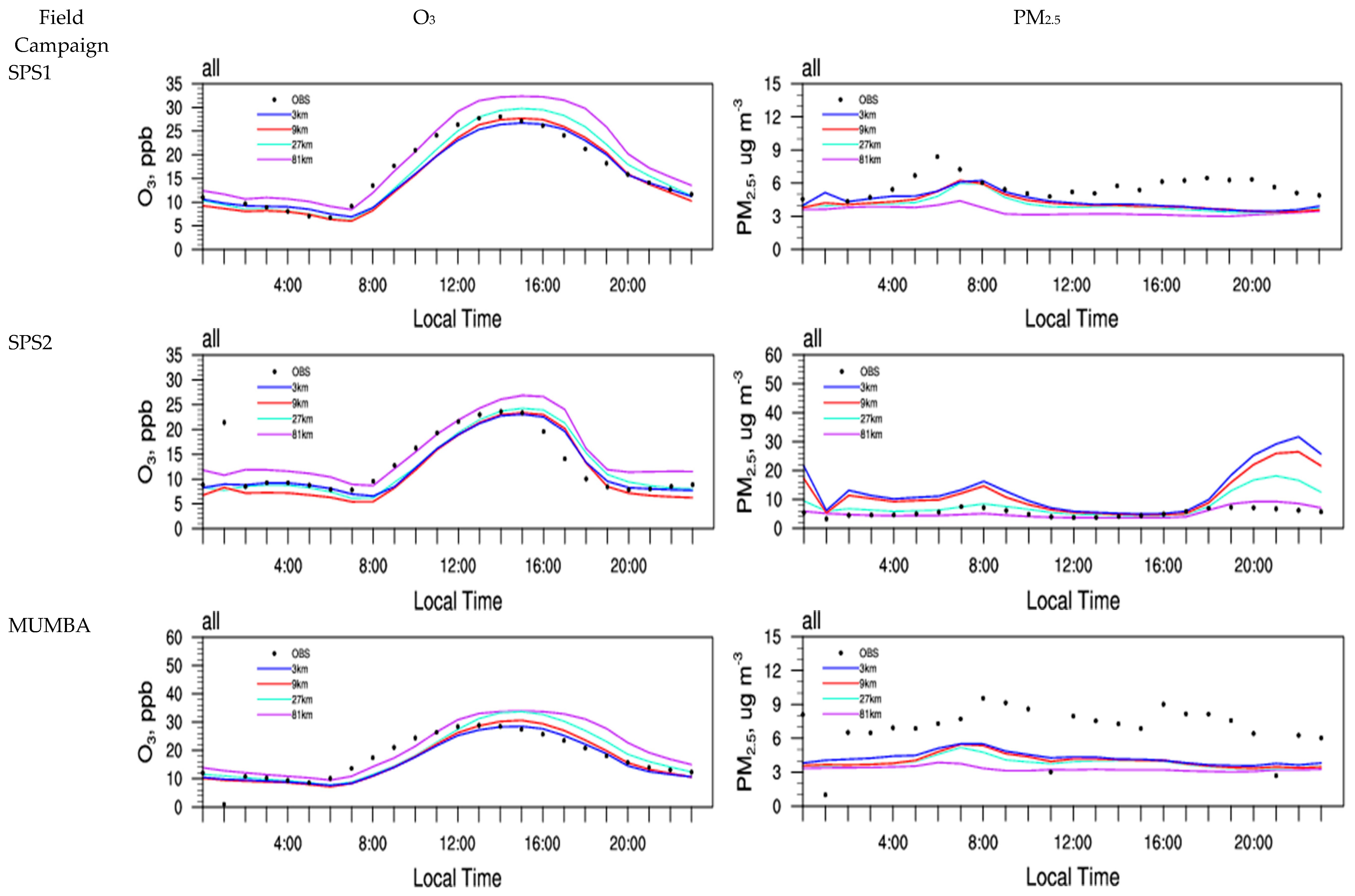
Figure 4 compares observed and simulated diurnal profiles of surface concentrations of O3 and PM2.5 from the WRF/Chem-ROMS simulations at various grid resolutions averaged over all monitoring stations over the Greater Sydney area (d04). The model performs similarly at 3-, 9-, and 27-km, which agrees better with observations than at 81-km. The underpredictions in O3 between 7 am and 1 pm are related to the underpredictions of T2 during the same hours as shown in Figure 3. The simulation at 81-km overpredicts O3 during all hours except 7–11 a.m. local time for SPS1 and MUMBA and 8 a.m.–12 p.m. local time for SPS2. The overpredictions at night are mainly caused by insufficient titration by NO (indicated by significant underpredictions of NO, see Table 1, Table 2 and Table 3). The large underpredictions of nighttime NO may be caused by underestimated NO emissions and also overpredicted nocturnal and morning PBL height (PBLH) as reported by Monk et al. [26]. Comparing to SPS1 and SPS2, the nocturnal PBLH is better captured for MUMBA, therefore the nighttime O3 predictions at various grid resolutions are closer to the observations for MUMBA than for SPS1 and SPS2. As the underpredictions of NO reduce with increased grid resolutions, the nighttime O3 predictions generally agree better with observations, with the best performance at 3-km. According to Monk et al. [28], the model can better simulate PBLH in the afternoons. As the grid resolutions increase, the model can better capture the atmospheric mixing (indicated by reduced underpredictions of CO, see Table 1, Table 2 and Table 3) and the concentrations of O3 precursors such as NO and NO2, leading to less overpredictions of O3 during afternoon hours, with the best performance at 3-km.
To assess the model’s capability at both regional and urban scales, Figure 5 shows simulated spatial distributions of surface concentrations of O3 from the WRF/Chem-ROMS simulations at 3- and 27-km overlaid with observations over the Greater Sydney area (d04). While 27-km represents a regional scale, and 3-km represents an urban scale. For SPS1, although the NMB at 27-km is smaller than that at 3-km (0.5% vs. −5.7%), the use of 3-km grid resolution can better capture the concentration gradients, with the lowest concentrations at Liverpool and Chullora, and the highest at Oakdale. The 3-km simulation also more accurately reproduces the O3 concentrations at three sites in the southwest of the Greater Sydney area, University of Wollongong (UOW), Wollongong, and Warrawong. For SPS2, the model simulation at 3-km reproduces the lowest concentrations at Liverpool and Westmead, the highest at Oakdale, as well as a lower concentration at UOW than those at Wollongong and Warrawong, all of which were not well captured by the simulation at 27-km, even though the NMB at 27-km is smaller than that at 3-km (−0.2% vs. −3.4%). For MUMBA, although the NMB at 27-km is smaller than that at 3-km (2.8% vs. −10.1%), the observed highest O3 concentrations occurred at Oakdale and Bargo, which are more accurately simulated by the simulation at 3-km than at 27-km, particularly at Oakdale. Similar to SPS1 and SPS2, the 3-km simulation better captures the observed O3 concentrations at UOW, Wollongong, and Warrawong.
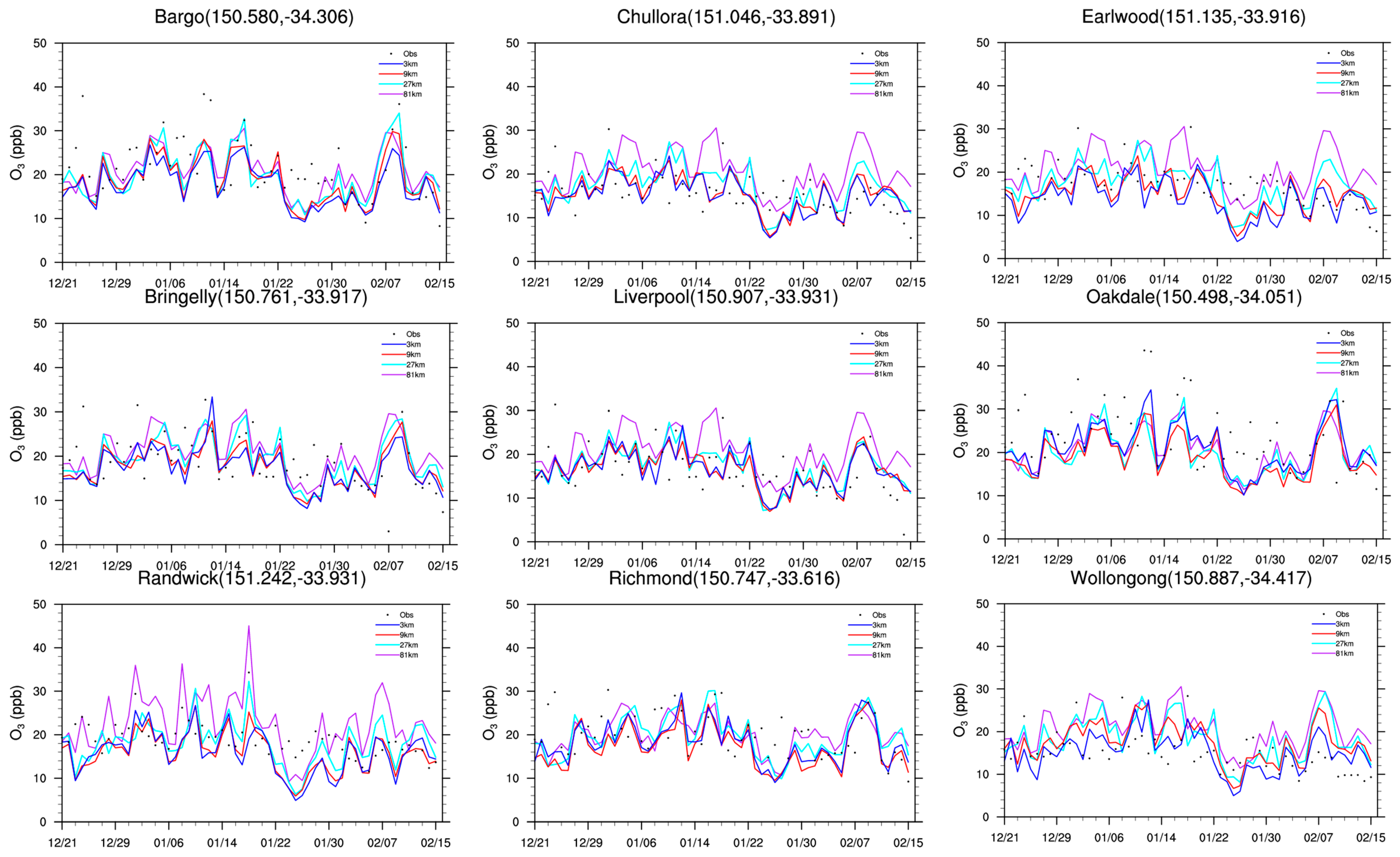
Figures S4 and S5 and Figure 6 compare observed and simulated temporal profiles of O3 concentrations from WRF/Chem-ROMS at selected sites during SPS1, SPS2, and MUMBA, respectively. The site-specific statistics is summarized in Table S1. For SPS1, the simulation at 81-km overpredicts O3 concentrations during most days at all sites, the simulation at 27-km gives the best performance at all sites, although all simulations miss the high O3 concentrations during Feb. 19–22 at most sites, especially at Oakdale. The highest observed O3 concentration (up to ~40 ppb) occured on Feb. 25 at Oakdale, which was underpredicted by all simulations. During SPS2, the O3 predictions show a much higher sensitivity to grid resolutions, especially at Randwick, Earlwood, Chullora, and Oakdale. The simulation at 81-km overpredicts O3 concentrations during most days except for Oakdale where all simulations underpredict O3 and for Wollongong where all simulations generally capture the magnitude of O3 well. The simulation at 27-km gives the best performance at all sites except for Oakdale and Randwick where the simulation at 3-km is the best and for Richmond where the simulation at 9-km is the best. Comparing to SPS1 and SPS2, the observed and simulated O3 concentrations during MUMBA show much stronger daily variations, driven by the strong daily variations of T2 shown in Figure S1. The simulation at 81-km tends to overpredict O3 during most days at Chullora, Earlwood, Liverpool, Randwick, and Wollongong. The simulation at 27-km gives the best performance at all sites except for Oakdale where the 3-km simulation is the best. All model simulations miss high O3 concentrations during Jan. 24–28 at most sites. Similar to SPS1, Oakdale has the highest observed O3 concentration (up to ~44 ppb) on Jan. 10–12, 2013 and O3 concentrations higher than 30 ppb on several days, which are underpredicted by all simulations. As shown in Table S1, the site-specific performance statistics is overall consistent with the domain-mean statistics. The simulated site-specific standard deviations generally agree with those based on observations during all three field campaigns.
As shown in Table 1, Table 2 and Table 3, for surface CO, the domain-mean NMBs are in the range of −66.3% to −54.9% at 81-km and −55.3% to −24.5% at finer grid resolutions. The moderate-to-large underpredictions in CO may be caused by underestimated CO emissions (because of the use the 2008 inventory, as discussed in Section 2.2) and overpredicted PBLHs. In addition, the use of a coarse grid resolution that causes greater CO underpredictions. Surface NO is significantly underpredicted with the domain-mean NMBs −89.3% to −77.3% at 81-km resolution. The model simulates NO better at finer grid resolutions, −44.6% to −18.1% at 27-km, −5.8% to 18.3% at 9-km, and 5.0–53.2% at 3-km resolution. For surface NO2, the model reproduces the observed seasonal variation well, with the highest observed NO2 concentrations during SPS2 comparing to those during SPS1 and MUMBA. Although photochemical production of NO2 is less during SPS2 than SPS1 and MUMBA due to weaker solar radiation in autumn than summer, the ventilation rates are lower in autumn than in summer, which favored the accumulation of NO2 in the Sydney basin. The domain-mean NMBs of NO2 are in the range of −32.3% to −29.5% at 81-km resolution, 0.7–6.2% at 27-km, 5.4–20.1% at 9-km, and 9.6–30.7% at 3-km resolution. Both NO and NO2 are affected by atmospheric mixing, emissions, and chemistry, and also highly sensitive to the grid resolution. The NO emissions are likely underestimated. While the use of finer grid resolutions effectively reduces NMBs of NO and NO2 concentrations for SPS1 and SPS2, it changes moderate-to-large underpredictions in NO and NO2 at 81-km (NMBs of −77.3% and −30.2%, respectively) to moderate-to-large overpredictions at 3-km (NMBs of 53.2% and 30.7%, respectively) for MUMBA. This indicates that high, localized NOx emissions are inadequately dispersed at 3-km (and 9-km to a lesser extent), resulting in overpredictions over the d04 domain. For surface SO2, the domain-mean NMBs at 81-, 27-, 9-, and 3-km are much higher, 50.7–114.3% for SPS1, 63.3–161.5% for SPS2, and 33.8–149.6% for MUMBA. Different from CO and NOx, increasing grid resolution leads to higher SO2 overpredictions with the highest at 3-km. While an overestimated SO2 emission (because of the use the 2008 inventory, as discussed in Section 2.2) and insufficient SO2 conversion to sulfate (indicated by underpredictions in precipitation) may be responsible in part for the overpredictions at all grid resolutions during all three field campaigns, the inadequate dispersion amplifies the model biases, resulting in much greater overpredictions at a finer grid resolution.
For surface PM2.5 and PM10, the model predicts the highest domain-mean concentrations in d04 at all grid resolutions during MUMBA (due mainly to its highest T2), followed by SPS1 and SPS2, which captures the observed seasonal variations. For PM2.5, most NMBs exceed the threshold value of 30% except for the simulations at 3–27 km for SPS1 and at 81-km for SPS2, and all NMEs exceed the threshold value of 50%, indicating a poor performance for PM2.5. Increasing grid resolution helps reduce NMBs for SPS1 and MUMBA but causes greater overpredictions for SPS2. The PM2.5 underpredictions during SPS1 and MUMBA may be caused by inaccurate meteorology (e.g., high biases in WS10), underestimated emissions (e.g., primary PM and PM2.5 precursors such as NOx and anthropogenic and biogenic VOCs), insufficient SO2 conversion to sulfate, and underprediction in secondary organic aerosol (SOA). The PM2.5 overpredictions during SPS2 may be caused by overpredictions of sulfate and organic carbon (OC) (which dominate PM2.5 concentrations), which may be attributed to overestimated emissions of SO2 (indicated by the large overprediction of SO2 concentrations) and primary OC. However, no OC observations are available to verify this speculation. 
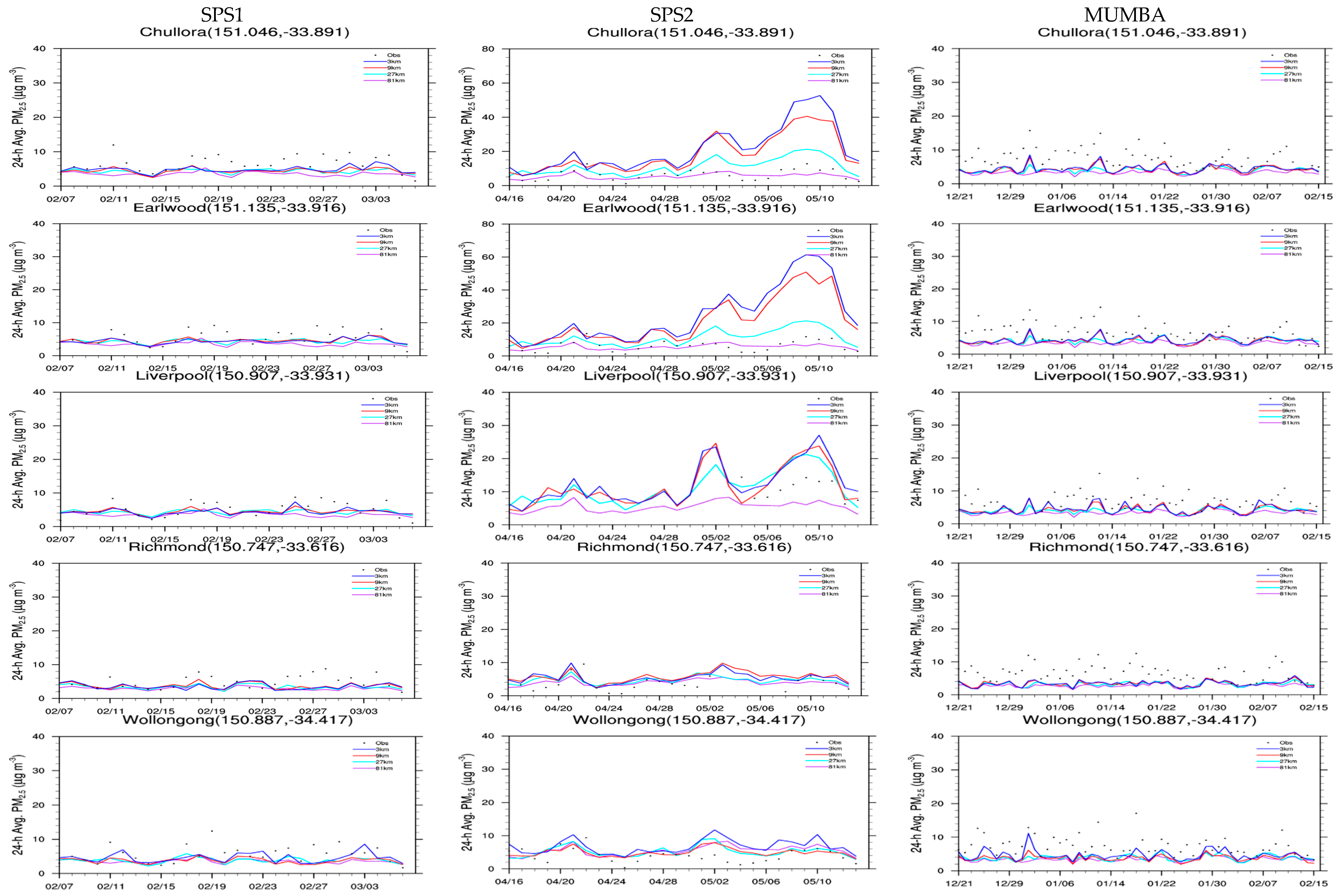
Figure 7 shows spatial distributions of surface concentrations of PM2.5 simulated by WRF/Chem-ROMS at 3- and 27-km resolutions overlaid with observations over the Greater Sydney area (d04). For SPS1 and MUMBA, the simulation at 3-km gives better statistical performance and also reproduces more accurately the observed concentration gradients at the five sites (Chullora, Earlwood, Liverpool, Richmond, and Wollongong) than the simulation at 27-km. For SPS2, the simulation at 3-km shows larger overpredictions than that at 27-km at all sites except for Richmond. Figure 8 compares observed and simulated temporal profiles of PM2.5 concentrations from WRF/Chem-ROMS at the five sites during SPS1, SPS2, and MUMBA. Table S2 summarizes site-specific performance statistics. During SPS1 and MUMBA, the PM2.5 underpredictions occur during most hours at all sites with the largest underpredictions at 81-km and the least underpredictions at 3-km. The differences among the simulations at different grid resolutions are relatively small during most hours at all sites. During SPS2, much larger differences for the four set of simulations occur at Chullora, Earlwood, and Liverpool compared to SPS1 and MUMBA, indicating a much higher sensitivity to grid resolution during autumn than during summer. However, the simulation at 81-km gives the best agreement to the observations, and the largest overpredictions occur at 3-km. As shown in Table S2, the site-specific performance statistics is overall consistent with the domain-mean statistics. However, the simulated site-specific standard deviations deviate from those based on observations during all three field campaigns, with the best agreement at 3-km for SPS1 and MUMBA but at 81-km for SPS2.
For surface PM10, observations are available at many more sites than PM2.5. Most NMBs exceed the threshold value of 30% except for the simulations at 3–27 km for SPS2, and all NMEs exceed the threshold value of 50%, indicating a poor performance for PM10. The large PM10 underpredictions during SPS1 and MUMBA may be caused by underpredictions of PM2.5 and underestimate of PM10 emissions (because of the use the 2008 inventory, as discussed in Section 2.2) and sea-salt emissions. The seemly better performance of PM10 at 3-, 9-, and 27-km grid resolutions during SPS2 is mainly because of large overpredictions of PM2.5. While the use of 3-km only improves the PM10 performance for SPS1 and MUMBA slightly, it reduces the NMBs for PM10 for SPS2 to a larger extent, but this is because of increased overpredictions in PM2.5 as the grid resolution increases. In addition to the aforementioned possible reasons for PM2.5 underpredictions that may also explain the moderate-to-large PM10 underpredictions, an additional reason may be the underpredictions in sea-salt emissions and concentrations. Figure 9 shows simulated spatial distribution of surface concentrations of PM10 by WRF/Chem-ROMS at 3- and 27-km overlaid with observations over the Greater Sydney area (d04). The simulations at 3-km reproduces better the observed PM10 concentration gradients for all three field campaigns than those at 27-km, particularly for SPS2. The moderate-to-large PM10 underpredictions occur at both inland and coastal sites for SPS1 and MUMBA, with larger underpredictions at inland sites.

3.3. Evaluation of Radiative, Cloud, and Heat flux Variables

Table 4, Table 5 and Table 6 summarizes the performance statistics of radiative, cloud, heat flux, and column gas variables simulated using WRF/Chem-ROMS for SPS1, SPS2, and MUMBA, respectively.
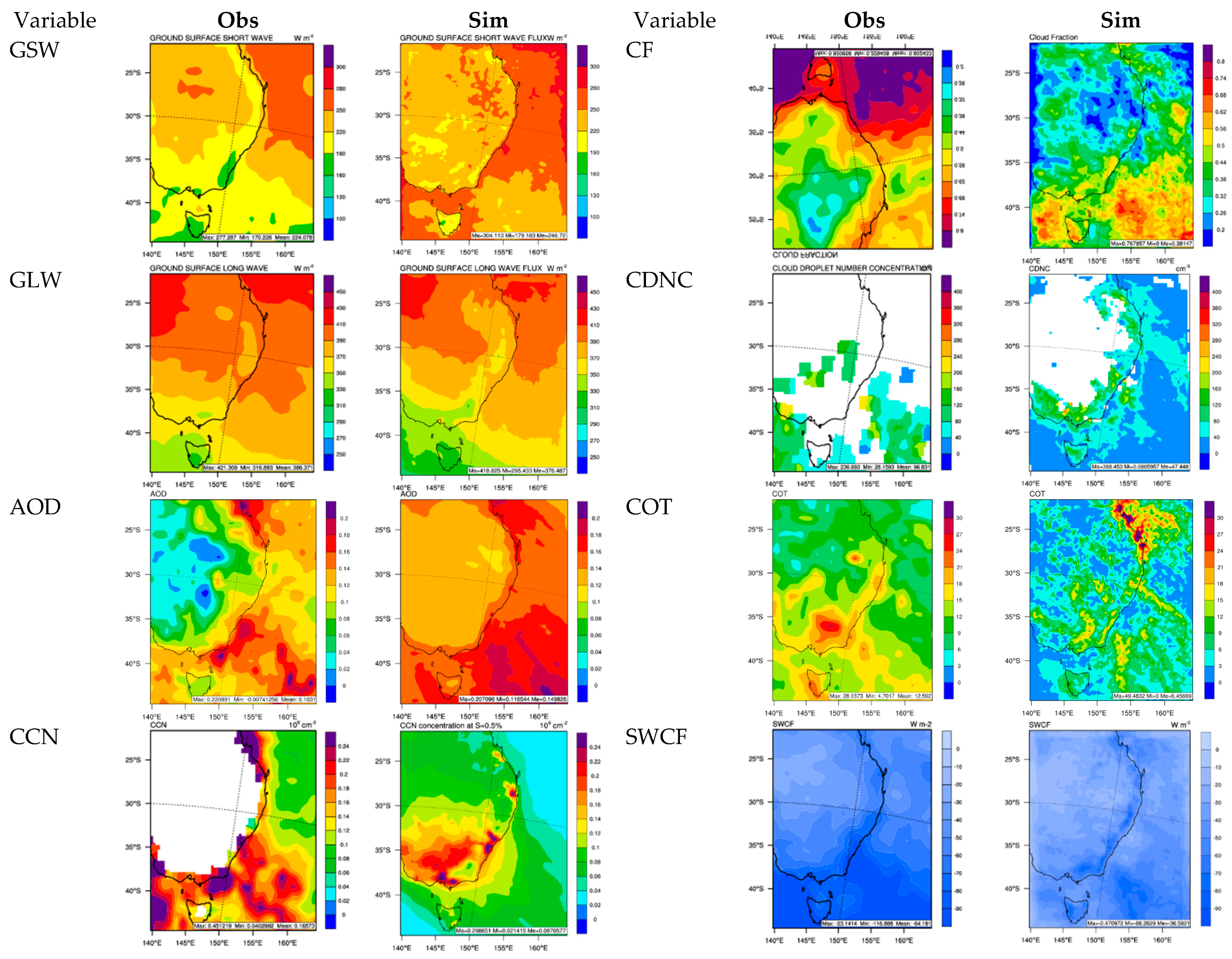
 Figure 10 and Figures S7 and S8 compare observed and WRF/Chem-ROMS simulated radiation and optical variables, CCN, and cloud variables at 27-km over d02. Comparing to PBL meteorological predictions, the radiation and cloud predictions are relatively less sensitive to grid resolution. For SPS1, the model simulates GLW well with NMBs within 5% but moderately overpredicts GSW with NMBs of 23–27.8%. As shown in Figure 10, the model does better in simulating observed gradients for GSW over the northern portion of d02 except along the coastal areas, it overpredicts GSW in the southern portion of d02. The model generally reproduces the spatial distributions and gradients of GLW well, despite underpredictions in the southern portion of d02. AOD is slightly overpredicted with NMBs of 1.6–8.3% over d04 at all grid resolutions, which is considered to be an excellent performance. The model gives similar spatial pattern to that of the MODIS AOD over oceanic areas but moderately overpredicts AOD over land areas in d02 (with an NMB of 45% over d02). CCN observations are only available over the ocean. CCN over the ocean is moderately underpredicted with NMBs ranging from −22.7% to −12.7%, especially in the northeastern and the southwestern portions of the d02. The underpredictions of CCN over the ocean are likely related to PM10 underpredictions, although no surface and column PM10 concentrations over the ocean are available for model evaluation. PWV is slightly underpredicted with NMBs of −12.1% to −11.6%, CF is moderately underpredicted with NMBs of −46.3% to −39.4%, and LWP is largely underpredicted with NMBs ranging from −96.8% to −89.1%. Simulated CF shows a similar pattern to observed CF with higher CF in the southern portion than the northern portion, but with much lower values in both land and ocean areas than observed CF. The underpredictions mostly occur in the southern portion of d02, in particular over the ocean areas. CDNC predictions are sensitive to grid resolution, with moderate underpredictions of 46.2% at 81-km and 31.2% at 3-km, but much better agreement with observations with an NMB of 3.5% at 27-km and −6.2% at 9-km. CDNC underpredictions can be attributed in part to the underpredictions of PM10 and uncertainties in the derived CDNC based on MODIS retrievals of cloud properties such as cloud effective radius, LWP, and COT, all of which are subject to uncertainties. COT is largely underpredicted with NMBs of −80.4% to −62.0%. Most underpredictions occur over land, particularly over the southern portion of the domain. Since COT depends on CDNC and LWP, the underpredictions in CDNC and CWP propagate into the COT predictions. In addition, the COT calculation in WRF/Chem-ROMS only accounts for contributions from water and ice, and contributions from other hydrometeors such as graupel are neglected, which explains in part the underpredictions of COT. The model largely underpredicts SWCF with NMBs of −60.4% to −47.8% and LWCF with NMBs of −55.1% to −40%. The spatial distributions of the observed SWCF correlate well with those of the observed CF, a similar correlation is found between simulated SWCF and CF, although it is weaker owing to underpredictions in both CF and SWCF. Such underpredictions in SWCF can be attributed to the underpredictions in CCN over the ocean and possibly over land, CDNC, LWP, and COT, caused by possible underpredictions in column PM10 concentrations. The model overpredicts LHF and SHF over the ocean against OAFlux data, with NMBs of 26.4–49.4% and 16.0–74.2%, respectively. Using finer grid resolutions of 3- or 9-km can reduce the model biases in simulating the latent and sensible heat flux.
For SPS2, the model simulates GLW and GSM well with NMBs within 3% and 13%, respectively. As shown in Figure S6, the model simulates well the spatial distribution of GLW and GSW throughout the domain. AOD is largely overpredicted with NMBs of 71.0–76.6% over both land and ocean areas, which may be caused by higher PM2.5 concentrations at the surface (see Table 2) and possibly above the surface. CCN over the ocean is moderately underpredicted with NMBs ranging from −28.2% to −24.1%, especially in the northeastern and the southwestern portions of the d02. PWV is moderately overpredicted with NMBs of 21.0–21.3%, CF is moderately underpredicted with NMBs of −32.2% to −25.9%, and LWP is largely underpredicted with NMBs ranging from −95.0% to −93.6%. As shown in Figure S7, similar to SPS1, the simulated CF shows a similar pattern to observed CF. Observed CDNC is available in a few areas in d02 but is not available over d04, thus there is no statistical evaluation over d04. COT is moderately to largely underpredicted with NMBs of −61.2% to −18.7%. Underpredictions occur over all land areas for the reasons discussed above. The model captures COT over oceanic areas well. The model underpredicts SWCF with NMBs of −31.1% to −4.1% and LWCF with NMBs of −34.5% to −9.8%. As shown in Figure S7, the simulated SWCF shows similar distributions as the observed SWCF. Unlike SPS1, the model tends to underpredict LHF and SHF over the ocean against OAFlux data, with NMBs of −19.9% to 1.8% and −45.3% to −22.9%, respectively. The 3-km simulation gives the best performance for both LHF and SHF.
For MUMBA, the model simulates GLW well with NMBs within 5% but moderately overpredicts GSW with NMBs of 21.7–25.8%. As shown in Figure S6, the underprediction of GSW occur over most of d02 except over the ocean areas in the southwestern portion. The model generally reproduces the spatial distribution and gradients of GLW well, despite underpredictions in the northern portion and overpredictions in the southwestern portion. AOD is moderately overpredicted with NMBs of 27.2–34.5%, which occurs over both land and ocean areas in the northern portion of d02. This AOD overprediction may be caused by higher PM2.5 concentrations above the surface as the surface PM2.5 concentrations are largely underpredicted (see Table 3). CCN over the ocean is largely underpredicted over all ocean areas with NMBs ranging from −57.9% to −54.4%. PWV is moderately overpredicted with NMBs of 17.7% to 18.6%, CF is largely underpredicted with NMBs of −65.8% to −48.7%, and LWP is largely underpredicted with NMBs ranging from −97.1% to −90.9%. As shown in Figure S7, simulated CF is much lower than observed CF especially over ocean areas. Similar to SPS2, observed CDNC is only available in a few areas in d02 but is not available over d04. COT is moderately to largely underpredicted with NMBs of −71.0% to −37.4%, mainly over land areas for the aforementioned reasons. The model captures COT over oceanic areas well. The model largely underpredicts SWCF with NMBs of −55.0% to −44.7% and LWCF with NMBs of −68.8% to −61.2%. As shown in Figure S7, the model is able to simulate the correlation between the spatial distributions of the observed SWCF and observed CF, but the simulated correlation is much weaker because of large underpredictions in both CF and SWCF. The model either overpredicts or underpredicts LHF and SHF over the ocean against OAFlux data, with NMBs of −9.9% to 8.1% and −35.5% to 7.3%, respectively. The better performance is at 27-km for LHF and at 81-km for SHF.

3.4. Evaluation of Column Gas Abundances

As shown in Table 4, Table 5 and Table 6, for column CO, the domain-mean NMBs and NMEs are very similar for the simulations at various grid resolutions, ranging from −22% to−21.4% and from 21.6% to 22.2%, respectively, for SPS1, from −7.3% to −6.8% and from 7.2% to 7.4%, respectively, for SPS2, and from −17.4% to −17.0% and from 17.4% to 17.1%, respectively, for MUMBA. Figure 11 compares observed and simulated column mass abundances of CO, NO2, HCHO, and O3 over d02. The underpredictions in CO column occur throughout the domain for SPS1 and MUMBA and mostly in the middle and southern part of the domain for SPS2. Such underpredictions are caused by moderate-to-large underpredictions of CO concentrations at surface (as shown in Table 1, Table 2 and Table 3) and aloft. The underpredictions are attributed to underestimated CO emissions, inaccurate chemical boundary conditions, and possible overestimated atmospheric mixing in the PBL either during daytime or nighttime. The convective boundary-layer height determined by the lidar backscatter measurements at Westmead is 900 m during daytime on 8 May 2012 [29] and between 500–1700 m during daytime and between 100–250 m at night during the whole SPS2 period [104]. WRF/Chem-ROMS gives good agreement for nocturnal mixing depth but tends to underpredict daytime PBLH at this site. Monk et al. [28] evaluated simulated PBLH from WRF/Chem-ROMS against estimated PBLH based on radiosonde measurement at Sydney Airport during SPS1, SPS2, and MUMBA. They found that WRF/Chem-ROMS tends to overpredict PBLH in the morning (by 22–184 m) but underpredict it in the afternoon (by 100–230 m). The impact of overpredicted PBLH in the morning may dominate over the underpredicted PBLH in the afternoon, because CO emissions are generally higher in the morning than in the afternoon.
The column NO2 shows strong sensitivity to the grid resolution. The domain-mean NMBs are in the range of −43.1% to −34.2% at 81-km, −30.9% to −21.6% at 27-km, −23.6% to −15.4% at 9-km, and −22.7% to −11.5% at 3-km resolution. As shown in Figure 11, although the model reproduces the hot spots in the southern portion of the d02, most underpredictions occur over land and are likely caused by underpredictions of NO2 concentrations above the surface. The use of finer grid resolutions reduces the NMBs of column NO2 for all field campaigns. The column HCHO is either slightly or not sensitive to the grid resolution. Its domain-mean NMBs at all grid resolutions indicate a moderate underprediction (−27.4% to −16.4%) for SPS1 and SPS2 but less underpredictions (−11.4% to −0.1%) for MUMBA. The underpredictions mostly occur in the southern portion of the land areas and over ocean areas for SPS1 and MUMBA, but over both land and ocean areas throughout the domain for SPS2, which are likely caused by underpredictions of HCHO concentrations at the surface and above. The column O3 is slightly sensitive to the grid resolution with slightly improved performance as the grid resolution increases. The domain-mean NMBs at all grid resolutions are 23.1–26.9% for SPS1, 4.3–5.2% SPS2, and 39.4–42.0% for MUMBA. Overpredictions occur in the southern portion, most parts, and throughout the domain for SPS1, SPS2, and MUMBA, respectively.

4. Conclusions

In this work, two advanced online-coupled meteorology-chemistry models—WRF/Chem and WRF/Chem-ROMS—are applied over quadruple-nested domains at grid resolutions of 81-, 27-, 9-, and 3-km over Australia, an area in southeastern Australia, an area in New South Wales (NSW), and Greater Sydney area, respectively, during three field campaign periods: SPS1, SPS2, and MUMBA. Comprehensive model evaluation is performed using surface observations from the field campaigns, satellite retrievals, and combined satellite data and reanalysis data. This paper evaluates the performance of WRF/Chem-ROMS against these data and the sensitivity of the model predictions to spatial grid resolutions. The model generally meets the satisfactory performance criteria for T2, RH2, and WD10 at spatial grid resolutions of 3-, 9-, and 27-km, WS10 at 3- and 9-km, and precipitation at all grid resolutions. An overall good performance for WS10 and WD10 at 3- and 9-km is because of the use of a fine grid resolution and a surface roughness correction algorithm. The model can capture the seasonal variations of T2, WS10, WD10, and precipitation well. At 3-, 9-, and 27-km, the model can reproduce the diurnal variations of T2 (even during the heatwave events in January 2013) and WS10 reasonably well with moderate biases in the mornings and evenings, due to the model’s limitation in accurately representing the daytime and nocturnal boundary layer as well as surface sensible and latent heat fluxes over land areas during those time periods. The model can reproduce well the observed hourly variations of T2 at 3-, 9-, and 27-km and those of WS10 at 3- and 9-km. It can also correctly predict the time of the heavy precipitation at most sites but largely underpredicts the magnitudes of the observed rainfall (except against GPCP for SPS2). Such underpredictions are attributed to the limitations of either the M09 double moment microphysics scheme or the MSKF cumulus parameterization.
The model simulations show moderate biases for surface concentrations of CO, NO, and NO2 at 3-, 9-, and 27-km, but significant overpredictions for SO2 with the lowest biases at 81-km. The SO2 overpredictions are attributed to several factors such as overestimated SO2 emissions, insufficient SO2 conversion to sulfate, and the inadequate dispersion at finer grid resolutions. The surface O3 predictions have NMBs within the good performance threshold (±15%) at all grid resolutions except at 81-km, despite the NMEs > 25%. While the PM2.5 prediction has an NMB within ±30% at all grid resolutions except at 81-km for SPS1, significant overpredictions for SPS2 and moderate-to-large underpredictions for MUMBA occur. In addition, all NMEs of PM2.5 exceed the threshold value of 50%. While the PM2.5 underpredictions may be attributed to inaccurate meteorology, underestimated emissions in NOx and anthropogenic and biogenic VOCs, insufficient SO2 conversion to sulfate, and underprediction in SOA, the PM2.5 overpredictions may be attributed to overestimations in emissions of SO2 and primary organic carbon. The model effectively reproduces the observed seasonal variations for all species except for SO2, which remains nearly constant. PM10 concentrations are largely underpredicted at 3-km in d04 during SPS1 and MUMBA, which may be caused by underpredictions of PM2.5 and underestimate of sea-salt emissions. The seemly good performance of PM10 for SPS2 results from large overpredictions in PM2.5. For spatial distribution, while the NMBs of O3 are the smallest at 27-km, the predictions at 3-km best resolve the spatial distributions and the maximum and minimum concentrations of O3 in d04. Compared to simulation at 27-km, the simulation at 3-km gives better statistical performance for PM2.5 and PM10 and also reproduces more accurately the observed concentration gradients over the d04 for SPS1 and MUMBA; it gives larger overpredictions for PM2.5 but smaller PM10 underpredictions for SPS2. For O3 and PM2.5 diurnal profiles, the model performs similarly at 3-, 9-, and 27-km with the best performance at 3-km, which agrees better with observations than at 81-km. For temporal variations, the model performs the best for O3 at 27-km during all three field campaigns and for PM2.5 at 3-km during SPS1 and MUMBA but at 81-km during SPS2.
For column variables, the model simulates GLW well, but moderately overpredicts GSW and either overpredicts or underpredicts PWV. LWCF, SWCF, and CF are slightly-to-moderately underpredicted during SPS2 but largely underpredicted during SPS1 and MUMBA. CCN is moderately underpredicted for SPS1 and SPS2 and largely underpredicted for MUMBA. The NMBs for COT and LWP are also very large. The overall poor performance of cloud variables indicates limitations in the model representation of cloud microphysics and dynamics. AOD is reproduced very well for SPS1, moderately overpredicted for SPS2, and largely overpredicted for MUMBA. The large overpredictions of AOD during SPS2 are caused by large overpredictions of PM2.5 at the surface and possibly aloft. LHF and SHF predictions show slight-to-moderate biases for SPS1 and MUMBA but moderate-to-large biases for SPS2. Column CO is slightly underpredicted for SPS2 but moderately underpredicted. The column NO2 is moderately underpredicted. The column HCHO is slightly underpredicted for MUMBA but moderately underpredicted. The column O3 is slightly overpredicted for SPS2 but moderately overpredicted for SPS1 and MUMBA.
All meteorological variables and surface chemical concentrations are sensitive to the spatial grid resolution used. WS10 and precipitation are more sensitive than T2, RH2, and WD10. The model has the worst performance at 81-km for most variables except for WD10 and SO2, for which the model performs the best at 81-km and RH2 and precipitation for which the model either performs the best or the second best at 81-km. While the use of finer grid resolutions can improve the model performance for most variables except for WD10, RH2, precipitation, and SO2, the model predictions at 3-, 9-, and 27-km are overall similar, and the best performance may happen at any grid resolutions due to the high non-linearity of the meteorological and chemical processes that affect the state and evolution of these variables. For example, the 3-km simulation gives the best performance for RH2, WS10, precipitation against MSWEP, CO, NO, PM2.5, and PM10 during SPS1, T2, SST, CO, and PM10 during SPS2, RH2, CO, PM2.5, and PM10 during MUMBA. The 9-km simulation performs the best for T2 and SST during SPS1, WS10, precipitation against GPCP, and NO during SPS2, and T2 and SST during MUMBA. The 27-km simulation performs the best for precipitation against OBS and GPCP, NO2, and O3 during SPS1, precipitation against OBS and MSWEP, NO2, and O3 during SPS2, and precipitation against GPCP, NO, NO2, and O3 during MUMBA. AOD, COT, CCN, CDNC, LHF, and SHF are moderately sensitive to the spatial grid resolution, and other radiative and cloud properties are relatively insensitive to the spatial grid resolution. Among column gas abundances, the column NO2 shows strong sensitivity to the grid resolution. The column CO, HCHO, and O3 are either slightly or not sensitive to the grid resolution. The 3- or 9-km simulations can reduce the biases for CCN, LHF, SHF, column NO2, and TOR during SPS1, AOD, CCN, column NO2, and TOR during SPS2, and CCN, column NO2, and TOR during MUMBA.
Several large differences are identified in the performance of WRF/Chem-ROMS or WRF/Chem for their applications in Australia compared to that for the continental U.S. (CONUS) and East Asia. First, the total precipitation is often overpredicted over CONUS and East Asia when the M09 cloud microphysics scheme is used together with any of the three cumulus parameterizations (e.g., Grell and Devenyi [101] (GD) or Grell and Freitas [102] or MSKF) [37,38,40,68] but underpredicted over Australia when MSKF is used. This indicates a need to further assess the parameters used in the MSKF scheme to understand why the convective precipitation is not triggered at a grid resolution of 3-km and also to pinpoint the reason underlying the underpredictions in precipitation. Second, the AOD is often underpredicted over CONUS [40,68] and East Asia [37,38] but is overpredicted in this work, especially for SPS2 and MUMBA. This indicates that the default initial and boundary conditions for PM species used in the simulation may have been higher than the actual values in Australia, and that more realistic initial and boundary conditions are needed for applications over Australia. While using satellite-constrained boundary conditions slightly reduces the overpredictions for SPS2 and MUMBA (see more details in the Part II paper), further improvement of boundary conditions for applications in Australia is warranted given its less polluted atmosphere than CONUS. Third, SST is slightly underpredicted (an MB of −0.8 °C) but LHF is moderately overpredicted (an NMB of 18.9%) and SHF is largely overpredicted (an NMB of 50.2%) over CONUS during summer time [40]. In this work, SST is slightly overpredicted during SPS1 (MBs of 0.5–1.0 °C) but slightly over- and under-predicted (MBs of −0.5 to 0.3°C) during MUMBA. LHF is slightly underpredicted (NMBs of −12.1% to −11.6%) and SHF is moderately overpredicted (NMBs of 23.4–38.2% at 3–27 km) during SPS1 but either slightly overpredicted or moderately underpredicted (−9.9% to 5.3% for LHF and −35.5 to −8.4% for SHF) during MUMBA. This indicates an overall better performance of WRF/Chem-ROMS in simulating SST, LHF, and SHF over the Pacific Ocean off the Australian coast than in the Atlantic Ocean off the southeastern U.S. coast.

Supplementary Materials

The following are available online at https://www.mdpi.com/2073-4433/10/4/189/s1, Figure S1: Observed and simulated temporal profiles of temperature at 2-m at selected sites during SPS1, SPS2, and MUMBA. All simulation results are based on WRF/Chem-ROMS. No observations are available at Bellambi during SPS2 and MUMBA. Figure S2: Observed and simulated temporal profiles of wind speed at 10-m at selected sites during SPS1, SPS2, and MUMBA. All simulation results are based on WRF/Chem-ROMS. No observations are available at Bellambi during SPS2 and MUMBA. Figure S3: Observed and simulated temporal profiles of precipitation at selected sites during SPS1, SPS2, and MUMBA. All simulation results are based on WRF/Chem-ROMS. Figure S4: Observed and simulated temporal profiles of O3 concentrations at selected sites during SPS1. All simulation results are based on WRF/Chem-ROMS. Figure S5: Observed and simulated temporal profiles of O3 concentrations at selected sites during SPS2. All simulation results are based on WRF/Chem-ROMS. Figure S6: Observed and simulated radiation and optical variables and CCN over southeastern Australia (d02) during SPS2 and MUMBA. The simulation results are from WRF/Chem-ROMS. Figure S7: Observed and simulated cloud variables over southeastern Australia (d02) during SPS2 and MUMBA. The simulation results are from WRF/Chem-ROMS. Table S1: Statistics of O3 for WRF/Chem-ROMS v3.7.1 simulations (81-km, 27-km, 9-km, and 3-km) over nine individual sites with 3-km domain. Table S2: Statistics of PM2.5 for WRF/Chem-ROMS v3.7.1 simulations (81-km, 27-km, 9-km, and 3-km) over five individual sites with 3-km domain.

Author Contributions

Conceptualization, Y.Z. and C.P.-W.; Methodology, Y.Z., J.D.S., and S.U.; Validation, C.J., K.W., and Y.Z.; Formal analysis, Y.Z.; Investigation, M.K.; Data curation, J.D.S., S.U., E.-A.G., K.W., and C.J.; Writing—original draft preparation, Y.Z.; Writing—review and editing, C.P.-W., S.U., and E.-A.G.; Funding acquisition, Y.Z. and C.P.-W.

Funding

This work was supported by the University of Wollongong (UOW) Vice Chancellors Visiting International Scholar Award (VISA), the University Global Partnership Network (UGPN), and the NC State Internationalization Seed Grant at North Carolina State University, U.S.A. and Australia’s National Environmental Science Program through the Clean Air and Urban Landscapes hub at University of Wollongong, Australia.

Acknowledgements

Simulations were performed on Stampede and Stampede 2, provided as an Extreme Science and Engineering Discovery Environment (XSEDE) digital service by the Texas Advanced Computing Center (TACC), and on Yellowstone (ark:/85065/d7wd3xhc) provided by NCAR’s Computational and Information Systems Laboratory, sponsored by the National Science Foundation.

Conflicts of Interest

The authors declare that they have no conflicts interests.

References

  1. Morgan, G.; Broome, R.; Jalaludin, B. Summary for Policy Makers of the Health Risk Assessment on Air Pollution in Australia. Available online: https://www.environment.gov.au/system/files/pages/dfe7ed5d-1eaf-4ff2-bfe7-dbb7ebaf21a9/files/summary-policy-makers-hra-air-pollution-australia.pdf (accessed on 6 April 2019).
  2. Keywood, M.D.; Emmerson, K.M.; Hibberd, M.F. Atmosphere: Atmosphere. In Australia State of the Environment 2016; Australian Government Department of the Environment and Energy: Canberra, Australia, 2016. Available online: https://soe.environment.gov.au/ (accessed on 6 April 2019). [CrossRef]
  3. Tanaka, T.Y.; Chiba, M. A numerical study of the contributions of dust source regions to the global dust budget. Glob. Planet. Chang. 2006, 52, 88–104. [Google Scholar] [CrossRef]
  4. Mackie, D.S.; Boyd, P.W.; McTainsh, G.H.; Tindale, N.W.; Westberry, T.K.; Hunter, K.A. Biogeochemistry of iron in Australian dust: From eolian uplift to marine uptake, Geochem. Geophys. Geosyst. 2008, 9, Q03Q08. [Google Scholar] [CrossRef]
  5. Gupta, P.; Christopher, S.A.; Box, M.A.; Box, G.P. Multi year satellite remote sensing of particulate matter air quality over Sydney. Aust. Int. J. Remote Sens. 2007, 28, 4483–4498. [Google Scholar] [CrossRef]
  6. Dirksen, R.J.; Folkert Boersma, K.; de Laat, J.; Stammes, P.; van der Werf, G.R.; Val Martin, M.; Kelder, H.M. An aerosol boomerang: Rapid around-the-world transport of smoke from the december 2006 Australian forest fires observed from space. J. Geophys. Res. Atmos. 2009, 114, D21201. [Google Scholar] [CrossRef]
  7. Higgenbotham, N.; Freeman, S.; Connor, L.; Albrecht, G. Environmental injustice and air pollution in coal affected communities, Hunter Valley, Australia. Health Place 2010, 16, 259–266. [Google Scholar] [CrossRef]
  8. Chakaraborty, J.; Green, D. Australia’s first national level quantitative environmental justice assessment of industrial air pollution. Environ. Res. Lett. 2014, 9, 044010. [Google Scholar] [CrossRef]
  9. Giglio, L.; Randerson, J.T.; van der Werf, G.R.; Kasibhatla, P.S.; Collatz, G.J.; Morton, D.C.; DeFries, R.S. Assessing variability and long-term trends in burned area by merging multiple satellite fire products. Biogeosciences 2010, 7, 1171–1186. [Google Scholar] [CrossRef]
  10. Paton-Walsh, C.; Emmons, L.K.; Wilson, S.R. Estimated total emissions of trace gases from the canberra wildfires of 2003: A new method using satellite measurements of aerosol optical depth & the mozart chemical transport model. Atmos. Chem. Phys. 2010, 10, 5739–5748. [Google Scholar]
  11. Paton-Walsh, C.; Emmons, L.; Wiedinmyer, C. Australia’s Black Saturday fires—Comparison of techniques for estimating emissions from vegetation fires. Atmos. Environ. 2012, 60, 262–270. [Google Scholar] [CrossRef]
  12. Rotstayn, L.D.; Collier, M.A.; Mitchell, R.M.; Qin, Y.; Campbell, S.K.; Dravitzki, S.M. Simulated enhancement of ENSO-related rainfall variability due to Australian dust. Atmos. Chem. Phys. 2011, 11, 6575–6592. [Google Scholar] [CrossRef]
  13. AAQ NEPM. Draft Variation to the National Environment Protection (Ambient Air Quality) Measure: Impact Statement; Appendix D; National Environment Protection Council, Department of the Environment: Canberra, Australia, July 2014; p. 42. Available online: https://www.environment.gov.au/protection/nepc/nepms/ambient-air-quality/variation-2014/impact-statement (accessed on 6 April 2019).
  14. Rea, G.; Paton-Walsh, C.; Turquety, S.; Cope, M.; Griffith, D. Impact of the New South Wales fires during October 2013 on regional air quality in eastern Australia. Atmos. Environ. 2016, 131, 150–163. [Google Scholar] [CrossRef]
  15. Duc, H.N.; Chang, L.T.-C.; Trieu, T.; Salter, D.; Scorgie, Y. Source Contributions to Ozone Formation in the New South Wales Greater Metropolitan Region, Australia. Atmosphere 2018, 9, 443. [Google Scholar] [CrossRef]
  16. Utembe, S.; Rayner, P.; Silver, J.; Guerette, E.-A.; Fisher, J.A.; Emmerson, K.; Cope, M.; Paton-Walsh, C.; Griffiths, A.D.; Duc, H.; et al. Hot summers: Effect of extreme temperatures on ozone in Sydney, Australia. Atmosphere 2018, 9, 466. [Google Scholar] [CrossRef]
  17. Begg, S.; Vos, T.; Barker, B.; Stevenson, C.; Stanley, L.; Lopez, A.D. The Burden of Disease and Injury in Australia 2003; Cat. No. PHE 82; Australian Institute of Health and Welfare: Canberra, Australia, 2007; p. 234. Available online: http://www.aihw.gov.au/publication-detail/?id=6442467990.BoM (accessed on 6 April 2019).
  18. AIHW (Australian Institute of Health and Welfare). Australian Burden of Disease Study: Impact and Causes of Illness and Death in Australia 2011; AIHW: Canberra, Australia, 2016.
  19. SCARC (Senate Community Affairs References Committee, Parliament of Australia). Impacts on Health of Air Quality in Australia; Senate Printing Unit, Parliament House: Canberra, Australia, 2013; p. 3.
  20. Broome, R.A.; Fann, N.; Cristina, T.J.; Fulcher, C.; Duc, H.; Morgan, G.G. The health benefits of reducing air pollution in Sydney, Australia. Environ. Res. 2015, 143, 19–25. [Google Scholar] [CrossRef]
  21. Keywood, M.D.; Galbally, I.; Crumeyrolle, S.; Miljevic, B.; Boast, K.; Chambers, S.D.; Cheng, M.; Dunne, E.; Fedele, R.; Gillett, R.; et al. Sydney Particle Study—Stage-I: Executive Summary; The Centre for Australian Weather and Climate Research: Aspendale, Australia, 2012.
  22. Cope, M.; Keywood, M.; Emmerson, K.; Galbally, I.; Boast, K.; Chambers, S.; Cheng, M.; Crumeyrolle, S.; Dunne, E.; Fedele, R.; et al. Sydney Particle Study—Stage-II; The Centre for Australian Weather and Climate Research: Aspendale, Australia, June 2014; ISBN 978-1-4863-0359-5.
  23. Paton-Walsh, C.; Guerette, E.; Kubistin, D.; Humphries, R.; Wilson, S.R.; Dominick, D.; Galbally, I.; Buchholz, R.; Bhujel, M.; Chambers, S.; et al. The MUMBA campaign: Measurements of urban, marine and biogenic air. Earth Syst. Sci. Data 2017, 9, 349–362. [Google Scholar] [CrossRef]
  24. Paton-Walsh, C.; Guerette, E.; Emmerson, K.; Cope, M.; Kubistin, D.; Humphries, R.; Wilson, S.R.; Buchholz, R.; Jones, N.B.; Griffith, D.W.T.; et al. Urban Air Quality in a Coastal City: Wollongong during the MUMBA Campaign. Atmosphere 2018, 9, 500. [Google Scholar] [CrossRef]
  25. BoM: Monthly Weather Review; Bureau of Meteorology: NSW, Sydney, Australia, February 2011.
  26. Chambers, S.; Williams, A.G.; Zahorowski, W.; Griffiths, A.; Crawford, J. Separating remote fetch and local mixing influences on vertical radon measurements in the lower atmosphere. Tellus B 2011, 63, 843–859. [Google Scholar] [CrossRef]
  27. White, C.J.; Fox-Hughes, P. Seasonal climate summary southern hemisphere (summer 2012–13): Austrlia’s hottest summer on record and extreme east coast rainfall. Aust. Meteorol. Oceanogr. J. 2013, 63, 443–456. [Google Scholar] [CrossRef]
  28. Monk, K.; Guérette, E.A.; Utembe, S.; Silver, J.D.; Emmerson, K.; Griffiths, A.; Duc, H.; Chang, L.T.C.; Trieu, T.; Jiang, N.; et al. Evaluation of regional air quality models over Sydney, Australia: Part 1 Meteorological model comparison. Atmosphere 2019. in review. [Google Scholar]
  29. Cope, M.E.; Hess, G.D.; Lee, S.; Tory, K.; Azzi, M.; Carras, J.; Lilley, W.; Manins, P.C.; Nelson, P.; Ng, L.; et al. The Australian Air Quality Forecasting System. Part I: Project description and early outcomes. J. Appl. Meteorol. 2004, 43, 649–662. [Google Scholar] [CrossRef]
  30. Guérette, E.-A.; Monk, K.; Emmerson, K.; Utembe, S.; Zhang, Y.; Silver, J.; Duc, H.N.; Chang, L.T.-C.; Trieu, T.; Griffiths, A.; et al. Evaluation of regional air quality models over Sydney, Australia: Part 2 Model performance for surface ozone and PM2.5. Atmosphere 2019. in preparation. [Google Scholar]
  31. Chang, L.T.-C.; Duc, H.N.; Scorgie, Y.; Trieu, T.; Monk, K.; Jiang, N. Performance evaluation of CCAM-CTM regional airshed modelling for the New South Wales Greater Metropolitan Region. Atmosphere 2018, 9, 486. [Google Scholar] [CrossRef]
  32. Grell, A.G.; Peckham, S.E.; Schmitz, R.; McKeen, S.A.; Frost, G.; Skamarock, W.C.; Eder, B. Fully coupled “online” chemistry within the WRF model. Atmos. Environ. 2005, 39, 6957–6975. [Google Scholar] [CrossRef]
  33. Zhang, Y.; Wen, X.-Y.; Jang, C.J. Simulating Chemistry–Aerosol–Cloud–Radiation–Climate Feedbacks over the Continental U.S. using the Online-Coupled Weather Research Forecasting Model with Chemistry (WRF/Chem). Atmos. Environ. 2010, 44, 3568–3582. [Google Scholar] [CrossRef]
  34. Zhang, Y.; Chen, Y.; Sarwar, G.; Schere, K. Impact of gas-phase mechanisms on Weather Research Forecasting Model with Chemistry (WRF/Chem) predictions: Mechanism implementation and comparative evaluation. J. Geophys. Res. 2012, 117, D01301. [Google Scholar] [CrossRef]
  35. Zhang, Y.; Karamchandani, P.; Glotfelty, T.; Streets, D.G.; Grell, G.; Nenes, A.; Yu, F.; Bennartz, R. Development and initial application of the global-through-urban weather research and forecasting model with chemistry (GU-WRF/Chem). J. Geophys. Res. 2012, 117, D20206. [Google Scholar] [CrossRef]
  36. Zhang, Y.; Sartelet, K.; Zhu, S.; Wang, W.; Wu, S.-Y.; Zhang, X.; Wang, K.; Tran, P.; Seigneur, C. Application of WRF/Chem-MADRID and WRF/Polyphemus in Europe, Part II: Evaluation of Chemical Concentrations and Sensitivity Simulations. Atmos. Chem. Phys. 2013, 13, 6845–6875. [Google Scholar] [CrossRef]
  37. Zhang, Y.; Zhang, X.; Wang, L.-T.; Zhang, Q.; Duan, F.-K.; He, K.-B. Application of WRF/Chem over East Asia: Part I. Model Evaluation and Intercomparison with MM5/CMAQ. Atmos. Environ. 2016, 124 Pt B, 285–300. [Google Scholar] [CrossRef]
  38. He, J.; Zhang, Y.; Wang, K.; Chen, Y.; Leung, L.R.; Fan, J.-W.; Li, M.; Zheng, B.; Zhang, Q.; Duan, F.-K.; et al. Multi-Year Application of WRF-CAM5 over East Asia-Part I: Comprehensive Evaluation and Formation Regimes of O3 and PM2.5. Atmos. Environ. 2017, 165, 122–142. [Google Scholar] [CrossRef]
  39. Vara-Vela, V.; Andrade, M.F.; Zhang, Y.; Kumar, P.; Ynoue, R.Y.; Souto-Oliveira, C.E.; Lopes, F.J.S.; Landulfo, E. Modelling of atmospheric aerosol properties in the Sao Paulo Metropolitan Area: The impact of biomass burning contribution. J. Geophys. Res. 2018, 123, 9935–9956. [Google Scholar] [CrossRef]
  40. He, J.; He, R.; Zhang, Y. Impacts of Air–sea Interactions on Regional Air Quality Predictions Using a Coupled Atmosphere-Ocean Model in Southeastern U.S. Aerosol Air Qual. Res. 2018, 18, 1044–1067. [Google Scholar] [CrossRef]
  41. Wang, K.; Yahya, K.; Zhang, Y.; Wu, S.-Y.; Grell, G. Implementation and Initial Application of A New Chemistry-Aerosol Option in WRF/Chem for Simulation of Secondary Organic Aerosols and Aerosol Indirect Effects. Atmos. Environ. 2015, 115, 716–732. [Google Scholar] [CrossRef]
  42. Yahya, K.; Glotfelty, T.; Wang, K.; Zhang, Y.; Nenes, A. Modeling Regional Air Quality and Climate: Improving Organic Aerosol and Aerosol Activation Processes in WRF/Chem version 3.7.1. Geosci. Model Dev. 2017, 10, 2333–2363. [Google Scholar] [CrossRef]
  43. Warner, J.C.; Armstrong, B.; He, R.; Zambon, J.B. Development of a coupled ocean-atmosphere-wave-sediment transport (COWAST) modeling system. Ocean Model. 2010, 35, 230–244. [Google Scholar] [CrossRef]
  44. Shchepetkin, A.F.; McWilliams, J.C. The Regional Ocean Modeling System: A split-explicit, free-surface, topography following coordinates ocean model. Ocean Model. 2005, 9, 347–404. [Google Scholar] [CrossRef]
  45. Marchesiello, P.; McWilliams, J.C.; Shchepetkin, A. Equilibrium structure and dynamics of the California current system. J. Phys. Oceanogr. 2003, 33, 753–783. [Google Scholar] [CrossRef]
  46. He, R.; Wilkin, J.L. Barotropic tides on the southeast New England shelf: A view from a hybrid data assimilative modeling approach. J. Geophys. Res. 2006, 111, C08002. [Google Scholar] [CrossRef]
  47. He, R.; McGillicuddy, D.J., Jr.; Keafer, B.A.; Anderson, D.M. Historic 2005 toxic bloom of Alexandrium fundyense in the western Gulf of Maine: 2. Coupled biological numerical modeling. J. Geophys. Res. 2008, 113, C07040. [Google Scholar] [CrossRef]
  48. Clough, S.A.; Shephard, M.W.; Mlawer, J.E.; Delamere, J.S.; Iacono, M.J.; Cady-Pereira, K.; Boukabara, S.; Brown, P.D. Atmospheric radiative transfer modeling: A summary of the AER codes. J. Quant. Spectrosc. Radiat. Transf. 2005, 91, 233–244. [Google Scholar] [CrossRef]
  49. Hong, S.-Y.; Noh, Y.; Dudhia, J. A new vertical diffusion package with an explicit treatment of entrainment processes. Mon. Weather Rev. 2006, 134, 2318–2341. [Google Scholar] [CrossRef]
  50. Hong, S.-Y. A new stable boundary-layer mixing scheme and its impact on the simulated East Asian summer monsoon. Q. J. R. Meteorol. Soc. 2010, 136, 1481–1496. [Google Scholar] [CrossRef]
  51. Chen, F.; Dudhia, J. Coupling an advanced land-surface/hydrology model with the Penn State/NCAR MM5 modeling system. Part I: Model implementation and sensitivity. Mon. Weather Rev. 2001, 129, 569–585. [Google Scholar] [CrossRef]
  52. Ek, M.B.; Mitchell, K.B.; Lin, Y.; Rogers, B.; Grunmann, P.; Koren, V.; Gayno, G.; Tarpley, J.D. Implementation of NOAH land surface model advances in the National Centers for Environmental Prediction operational mesoscale Eta model. J. Geophys. Res. 2003, 108, 8851. [Google Scholar] [CrossRef]
  53. Morrison, H.; Thompson, G.; Tatarskii, V. Impact of cloud microphysics on the development of trailing stratiform precipitation in a simulated squall line: Comparison of one- and two-moment schemes. Mon. Weather Rev. 2009, 137, 991–1007. [Google Scholar] [CrossRef]
  54. Zheng, Y.; Alapaty, K.; Herwehe, J.; Del Genio, A.; Niyogi, D. Improving high-resolution weather forecasts using the Weather Research and Forecasting (WRF) model with an updated Kain–Fritsch scheme. Mon. Weather Rev. 2016, 144, 833–860. [Google Scholar] [CrossRef]
  55. Yarwood, G.; Rao, S.; Yocke, M.; Whitten, G.Z. Final Report—Updates to the Carbon Bond Chemical Mechanism: CB05; Rep. RT-04-00675; Yocke and Co.: Novato, CA, USA, 2015; 246p. [Google Scholar]
  56. Sarwar, G.; Luecken, D.; Yarwood, G. Chapter 2.9: Developing and implementing an updated chlorine chemistry into the community multiscale air quality model. Dev. Environ. Sci. 2007, 6, 168–176. [Google Scholar] [CrossRef]
  57. Ahmadov, R.; McKeen, S.A.; Robinson, A.L.; Bareini, R.; Middlebrook, A.M.; De Gouw, J.A.; Meagher, J.; Hsie, E.-Y.; Edgerton, E.; Shaw, S.; et al. A volatility basis set model for summertime secondary organic aerosols over the eastern United States in 2006. J. Geophys. Res. 2012, 117. [Google Scholar] [CrossRef]
  58. Sarwar, G.; Fahey, K.; Napelenok, S.; Roselle, S.; Mathur, R. Examining the impact of CMAQ model updates on aerosol sulfate predictions. In Proceedings of the 10th Annual CMAS Models-3 User’s Conference, Chapel Hill, NC, USA, 24–26 October 2011. [Google Scholar]
  59. Abdul-Razzak, H.; Ghan, S. A parameterization of aerosol activation: 2. Multiple aerosol types. J. Geophys. Res. 2000, 105, 6837–6844. [Google Scholar] [CrossRef]
  60. Abdul-Razzak, H.; Ghan, S.J. A parameterization of aerosol activation, 3, Sectional representation. J. Geophys. Res. 2002, 107, 4026. [Google Scholar] [CrossRef]
  61. Chapman, E.G.; Gustafson, W.I., Jr.; Easter, R.C.; Barnard, J.C.; Ghan, S.J.; Pekour, M.S.; Fast, J.D. Coupling aerosol-cloud-radiative processes in the WRF-Chem model: Investigating the radiative impact of elevated point sources. Atmos. Chem. Phys. 2009, 9, 945–964. [Google Scholar] [CrossRef]
  62. Ghan, S.J.; Leung, L.R.; Easter, R.C.; Abdul-Razzak, H. Prediction of cloud droplet number in a general circulation model. J. Geophys. Res. 1997, 112, 21777–21794. [Google Scholar] [CrossRef]
  63. Liu, Y.; Daum, P.H.; McGraw, R.L. Size truncation effect, threshold behavior, and a new type of autoconversion parameterization. Geophys. Res. Lett. 2005, 32, L11811. [Google Scholar] [CrossRef]
  64. Chen, F.; Miao, S.; Tewari, M.; Bao, J.-W.; Kusaka, H. A numerical study of interactions between surface forcing and sea breeze circulations and their effects on stagnation in the greater Houston area. J. Geophys. Res. 2011, 116, D12105. [Google Scholar] [CrossRef]
  65. Seo, H.; Subramanian, A.C.; Miller, A.J.; Cavanaugh, N.R. Coupled Impacts of the Diurnal Cycle of Sea Surface Temperature on the Madden–Julian Oscillation. J. Clim. 2014, 27, 8422–8443. [Google Scholar] [CrossRef]
  66. Yahya, K.; Wang, K.; Gudoshava, M.; Glotfelty, T.; Zhang, Y. Application of WRF/Chem over North America under the AQMEII Phase 2. Part I. Comprehensive Evaluation of 2006 Simulation. Atmos. Environ. 2014, 115, 733–755. [Google Scholar] [CrossRef]
  67. Yahya, K.; Wang, K.; Zhang, Y.; Kleindienst, T.E. Application of WRF/Chem over North America under the AQMEII Phase 2—Part 2: Evaluation of 2010 application and responses if air quality and meteorology–chemistry interactions to changes in emissions and meteorology from 2006 to 2010. Geosci. Model Dev. 2015, 8, 2095–2117. [Google Scholar] [CrossRef]
  68. Yahya, K.; Wang, K.; Campbell, P.; Chen, Y.; Glotfelty, T.; He, J.; Pirhalla, M.; Zhang, Y. Decadal Application of WRF/Chem for Regional Air Quality and Climate Modeling over the U.S. under the Representative Concentration Pathways Scenarios. Part 1: Model Evaluation and Impact of Downscaling. Atmos. Environ. 2017, 152, 562–583. [Google Scholar] [CrossRef]
  69. Yahya, K.; Campbell, P.; Zhang, Y. Decadal Application of WRF/Chem for Regional Air Quality and Climate Modeling over the U.S. under the Representative Concentration Pathways Scenarios. Part 2: Current vs. Future simulations. Atmos. Environ. 2017, 152, 584–604. [Google Scholar] [CrossRef]
  70. Thiébaux, H.J.; Rogers, E.; Wang, W.; Katz, B. A new high-resolution blended real-time global sea surface temperature analysis. Bull. Am. Meteorol. Soc. 2003, 84, 645–656. [Google Scholar] [CrossRef]
  71. Reynolds, R.W.; Smith, T.M.; Liu, C.; Chelton, D.B.; Casey, K.S.; Schlax, M.G. Daily high-resolution-blended analyses for sea surface temperature. J. Clim. 2007, 40, 5473–5496. [Google Scholar] [CrossRef]
  72. EPA. 2008 Calendar Year Air Emissions Inventory for the Greater Metropolitan Region in NSW. Available online: https://www.epa.nsw.gov.au/your-environment/air/air-emissions-inventory/airemissions-inventory-2008 (accessed on 1 March 2018).
  73. Guenther, A.; Kart, T.; Harley, P.; Wiedinmyer, C.; Palmer, P.I.; Geron, C. Estimates of global terrestrial isoprene emissions using MEGAN (Model of Emissions of Gases and Aerosols from Nature). Atmos. Chem. Phys. 2006, 6, 3181–3210. [Google Scholar] [CrossRef]
  74. Jones, S.; Creighton, G. AFWA dust emission scheme for WRF/Chem-GOCART. In Proceedings of the 2011 WRF Workshop, Boulder, CO, USA, 20–24 June 2011. [Google Scholar]
  75. Gong, S.; Barrie, L.A.; Blanchet, J.P. Modeling sea salt aerosols in the atmosphere: 1. Model development. J. Geophys. Res. 1997, 102, 3805–3818. [Google Scholar] [CrossRef]
  76. Gantt, B.; He, J.; Zhang, X.; Zhang, Y.; Nenes, A. Incorporation of advanced aerosol activation treatments into CESM/CAM5: Model evaluation and impacts on aerosol indirect effects. Atmos. Chem. Phys. 2014, 14, 7485–7497. [Google Scholar] [CrossRef]
  77. He, J.; Zhang, Y. Improvement and Further Development in CESM/CAM5: Gas-Phase Chemistry and Inorganic Aerosol Treatments. Atmos. Chem. Phys. 2014, 14, 9171–9200. [Google Scholar] [CrossRef]
  78. Glotfelty, T.; He, J.; Zhang, Y. Impact of Future Climate Policy Scenarios on Air Quality and Aerosol/Cloud Interactions using an Advanced Version of CESM/CAM5: Part I. Model Evaluation for the Current Decadal Simulations. Atmos. Environ. 2017, 152, 222–239. [Google Scholar] [CrossRef]
  79. Beck, H.E.; van Dijk, A.I.J.M.; Levizzani, V.; Schellekens, J.; Miralles, D.G.; Martens, B.; de Roo, A. MSWEP: 3-hourly 0.25 global gridded precipitation (1979–2015) by merging gauge, satellite, and reanalysis data. Hydrol. Earth Syst. Sci. 2017, 21, 589–615. [Google Scholar] [CrossRef]
  80. Bennartz, R. Global assessment of marine boundary layer cloud droplet number concentration from satellite. J. Geophys. Res. 2007, 112, D02201. [Google Scholar] [CrossRef]
  81. Yu, L.; Jin, X.; Weller, R.A. Multidecade Global Flux Datasets from the Objectively Analyzed Air–Sea Fluxes (OAFlux) Project: Latent and Sensible Heat Fluxes, Ocean Evaporation, and Related Surface Meteorological Variables; OAFlux Project Technical Report, OA-2008-01; Woods Hole Oceanographic Institution: Woods Hole, MA, USA, 2008; 64p, Available online: http://oaflux.whoi.edu/pdfs/OAFlux_TechReport_3rd_release.pdf (accessed on 6 April 2019).
  82. Emery, C.; Tai, E. Enhanced Meteorological Modeling and Performance Evaluation for Two Texas Ozone Episodes; Project Report Prepared for the Texas Natural Resource Conservation Commission; ENVIRON International Corporation: Novato, CA, USA, 2001. [Google Scholar]
  83. Tesche, T.W.; Tremback, C. Operational Evaluation of the MM5 Meteorological Model over the Continental United States: Protocol for Annual and Episodic Evaluation; Draft Protocol Prepared under Task Order 4TCG-68027015 for the Office of Air Quality Planning and Standards; U.S. Environmental Protection Agency: Research Triangle Park, NC, USA, 2002.
  84. Wu, S.-Y.; Krishnan, S.; Zhang, Y.; Aneja, V. Modeling Atmospheric Transport and Fate of Ammonia in North Carolina, Part I. Evaluation of Meteorological and Chemical Predictions. Atmos. Environ. 2008, 42, 3419–3436. [Google Scholar] [CrossRef]
  85. Zhang, Y.; Liu, P.; Pun, B.; Seigneur, C. A Comprehensive Performance Evaluation of MM5-CMAQ for the Summer 1999 Southern Oxidants Study Episode, Part-I. Evaluation Protocols, Databases and Meteorological Predictions. Atmos. Environ. 2006, 40, 4825–4838. [Google Scholar] [CrossRef]
  86. Zhang, Y.; Cheng, S.-H.; Chen, Y.-S.; Wang, W.-X. Application of MM5 in China: Model Evaluation, Seasonal Variations, and Sensitivity to Horizontal Grid Resolutions. Atmos. Environ. 2011, 45, 3454–3465. [Google Scholar] [CrossRef]
  87. Penrod, A.; Zhang, Y.; Wang, K.; Wu, S.-Y.; Leung, R.L. Impacts of future climate and emission changes on U.S. air quality. Atmos. Environ. 2014, 89, 533–547. [Google Scholar] [CrossRef]
  88. Yahya, K.; He, J.; Zhang, Y. Multiyear Applications of WRF/Chem over Continental U.S.: Model Evaluation, Variation Trend, and Impacts of Boundary Conditions. J. Geophys. Res. 2015, 120, 12748–12777. [Google Scholar] [CrossRef]
  89. Wang, K.; Zhang, Y.; Zhang, X.; Fan, J.-W.; Leung, L.R.; Zheng, B.; Zhang, Q.; He, K.-B. Fine-Scale Application of WRF-CAM5 during a dust storm episode over East Asia: Sensitivity to grid resolutions and aerosol activation parameterizations. Atmos. Environ. 2018, 176, 1–20. [Google Scholar] [CrossRef]
  90. Zhang, Y.; Liu, P.; Queen, A.; Misenis, C.; Pun, B.; Seigneur, C.; Wu, S.-Y. A Comprehensive Performance Evaluation of MM5-CMAQ for the Summer 1999 Southern Oxidants Study Episode, Part-II. Gas and Aerosol Predictions. Atmos. Environ. 2006, 40, 4839–4855. [Google Scholar] [CrossRef]
  91. Yu, S.; Eder, B.; Dennis, R.; Chu, S.-H.; Schwartz, S. New unbiased symmetric metrics for evaluation of air quality models. Atmos. Sci. Lett. 2006, 7, 26–34. [Google Scholar] [CrossRef]
  92. Zhang, Y.; Wen, X.-Y.; Wang, K.; Vijayaraghavan, K.; Jacobson, M.Z. Probing into Regional Ozone and Particulate Matter Pollution in the United States: 2. An Examination of Formation Mechanisms Through A Process Analysis Technique and Sensitivity Study. J. Geophys. Res. 2009, 114, D22305. [Google Scholar] [CrossRef]
  93. Hogrefe, C.; Hao, W.; Civerolo, K.; Ku, J.Y.; Sistla, G.; Gaza, R.S.; Sedefian, L.; Schere, K.; Gilliland, A.; Mathur, R. Daily simulation of ozone and fine particulates over New York State: Findings and challenges. J. Appl. Meteorol. Climatol. 2007, 46, 961–979. [Google Scholar] [CrossRef]
  94. Emery, C.; Jung, J.; Downey, N.; Johnson, J.; Jimenez, M.; Yarwood, G.; Morris, R. Regional and global modeling estimates of policy relevant background ozone over the United States. Atmos. Environ. 2002, 47, 206–217. [Google Scholar] [CrossRef]
  95. Emery, C.; Liu, Z.; Russell, A.G.; Odman, M.T.; Yarwood, G.; Kumar, N. Recommendations on statistics and benchmarks to assess photochemical model performance. J. Air Waste Manag. Assoc. 2017, 67, 582–598. [Google Scholar] [CrossRef]
  96. Mass, C.; Ovens, D. WRF model physics: Problems, solutions and a new paradigm for progress. In Proceedings of the 2010 WRF Users’ Workshop, Boulder, CO, USA, 15–21 June 2010. [Google Scholar]
  97. Zhang, H.; Chen, G.; Hu, J.; Chen, S.H.; Wiedinmyer, C.; Kleeman, M.; Ying, Q. Evaluation of a seven-year air quality simulation using the Weather Research and Forecasting (WRF)/Community Multiscale Air Quality (CMAQ) models in the eastern United States. Sci. Total Environ. 2014, 473–474, 275–285. [Google Scholar] [CrossRef]
  98. Storm, B.; Dudhia, J.; Basu, S.; Swift, A.; Giammanco, I. Evaluation of the weather research and forecasting model on forecasting low-level jets: Implications for wind energy. Wind Energy 2009, 12, 81–90. [Google Scholar] [CrossRef]
  99. Shin, H.H.; Hong, S.Y. Intercomparison of planetary boundary layer parametrizations in the WRF model for a single day from CASES-99. Bound.-Layer Meteorol. 2011, 139, 261–281. [Google Scholar] [CrossRef]
  100. Draxl, C.; Hahmann, A.N.; Peña, A.; Giebel, G. Evaluating winds and vertical wind shear from Weather Research and Forecasting model forecasts using seven planetary boundary layer schemes. Wind Energy 2012, 17, 39–55. [Google Scholar] [CrossRef]
  101. Grell, G.A.; Devenyi, D. A generalized approach to parameterizing convection combining ensemble and data assimilation techniques. Geophys. Res. Lett. 2002, 29, 34–38. [Google Scholar] [CrossRef]
  102. Grell, G.A.; Freitas, S.R. A scale and aerosol aware stochastic convective parameterization for weather and air quality modeling. Atmos. Chem. Phys. 2014, 14, 5233–5250. [Google Scholar] [CrossRef]
  103. Wang, K.; Zhang, Y.; Yahya, K. Decadal application of WRF/Chem under current and future climate/emission scenarios, Part I: Comprehensive Evaluation and Intercomparison with Results under the RCP scenarios. 2019; in preparation. [Google Scholar]
  104. Chambers, S.D.; Guérette, E.-A.; Monk, K.; Griffiths, A.D.; Zhang, Y.; Duc, H.; Cope, M.; Emmerson, K.M.; Chang, L.T.; Silver, J.D.; et al. Skill-Testing Chemical Transport Models across Contrasting Atmospheric Mixing States Using Radon-222. Atmosphere 2019, 10, 25. [Google Scholar] [CrossRef]
Figure 1. Quadruple-nested modeling domains over Australia at 81-km (d01), southeastern Australia at 27-km (d02), New South Wales at 9-km (d03), and the Greater Sydney at 3-km (d04).
Atmosphere 10 00189 g001
Figure 2. Meteorological air quality monitoring stations over the Greater Sydney (d04).
Atmosphere 10 00189 g002
Figure 3. Observed and simulated diurnal profiles of temperature at 2-m (T2) and wind speed at 10-m (WS10) averaged over all meteorological monitoring stations maintained by the Bureau of Meteorology. All simulation results are based on WRF/Chem-ROMS.
Atmosphere 10 00189 g003
Figure 4. Observed and simulated diurnal profiles of surface concentrations of O3 and PM2.5 averaged over all monitoring stations over the Greater Sydney (d04). All simulation results are based on WRF/Chem-ROMS.
Atmosphere 10 00189 g004
Figure 5. Simulated spatial distribution of surface concentrations of O3 overlaid with observations over the Greater Sydney area (d04). All simulation results are based on WRF/Chem-ROMS.
Atmosphere 10 00189 g005
Figure 6. Observed and simulated temporal profiles of O3 concentrations at selected sites during MUMBA. All simulation results are based on WRF/Chem-ROMS.
Atmosphere 10 00189 g006
Figure 7. Simulated spatial distribution of surface concentrations of PM2.5 overlaid with observations over the Greater Sydney area (d04). All simulation results are based on WRF/Chem-ROMS.
Atmosphere 10 00189 g007
Figure 8. Observed and simulated temporal profiles of PM2.5 concentrations at selected sites during SPS1, SPS2, and MUMBA. All simulation results are based on WRF/Chem-ROMS.
Atmosphere 10 00189 g008
Figure 9. Simulated spatial distribution of surface concentrations of PM10 overlaid with observations over the Greater Sydney area (d04). All simulation results are based on WRF/Chem-ROMS.
Atmosphere 10 00189 g009
Figure 10. Observed and simulated radiation and optical variables and CCN over southeastern Australia (d02) during SPS1. The simulation results are from WRF/Chem-ROMS.
Atmosphere 10 00189 g010
Figure 11. Observed and simulated column mass abundances over southeastern Australia (d02). The simulation results are from WRF/Chem-ROMS.
Atmosphere 10 00189 g011
Table 1. Performance statistics of meteorological and chemical variables from WRF/Chem-ROMS simulations at a horizontal grid resolution of 81-km (in d01), 27-km (in d02), 9-km (in d03), and 3-km (in d04) calculated using predictions and observations in d04 for the SPS1 field campaign.
VariablesMean ObsMean SimRMBNMB, %NME, %
d01d02d03d04d01d02d03d04d01d02d03d04d01d02d03d04d01d02d03d04
Met
T2 (°C)22.121.221.922.122.20.850.860.860.86−0.9−0.220.020.09−4.1−1.00.10.49.48.67.97.8
SST (°C)23.925.324.924.424.50.3−0.3−0.50.41.41.00.50.65.94.22.32.95.94.23.12.9
RH2 (%)70.570.068.668.869.80.700.730.760.77−0.53−1.95−1.71−0.7−0.7−2.8−2.4−1.014.213.512.411.9
WS10 (m s−1)3.673.112.883.323.580.440.550.660.67−0.56−0.80−0.35−0.09−15.3−21.7−9.7−2.448.946.540.539.6
WD10 (°)150.6153.0160.1161.9160.10.790.830.830.832.409.5311.39.51.66.37.56.332.630.030.930.5
Precip (OBS) (mm day−1)0.840.960.840.660.870.260.200.060.090.12−0.01−0.180.0314.1−0.7−21.53.5150.9148.3146.8159.5
Precip. (MSWEP) (mm day−1)1.180.870.820.731.020.370.210.060.08−0.31−0.36−0.45−0.16−26.4−30.5−38.2−13.4103.1106.6112.6131.5
Precip (GPCP) (mm day−1)2.20.90.90.70.80.10.10.1−0.1−1.3−1.3−1.5−1.4−59.1−56.4−69.6−62.260.057.969.766.4
Chem
O3 (ppb)17.020.017.115.916.10.690.730.720.712.960.09−1.14−0.9717.40.5−6.7−5.742.437.036.836.5
CO (ppb)330.6121.2163.7147.9184.20.260.180.140.07−209.4−166.9−182.7−146.4−63.3−46.6−55.3−44.364.162.566.576.0
NO (ppb)4.860.753.304.585.110.180.280.330.30−4.11−1.56−0.280.26−84.5−32.0−5.85.094.6103.6113.5120.4
NO2 (ppb)6.334.296.376.676.940.380.520.490.52−2.050.040.340.61−32.30.75.49.664.358.761.462.0
SO2 (ppb)0.610.921.231.191.310.130.210.210.210.310.620.580.7050.7100.994.9114.3158.1189.5186.6200.8
PM2.5 (μg m−3)5.723.424.054.204.360.010.140.270.24−2.30−1.66−1.51−1.36−40.2−29.1−26.5−23.755.952.750.852.0
PM10 (μg m−3)17.87.27.97.98.40.040.150.240.20−10.6−9.9−9.8−9.4−59.4−55.6−55.4−52.962.859.658.559.0
Mean Obs and Sim: Time average across all grids with observations in each domain based on either hourly or daily predictions and observations, respectively; R: correlation coefficient; MB: mean bias; NMB: normalized mean bias; NME: normalized mean error; T2: 2-m temperature; SST: sea surface temperature; RH2: 2-m relative humidity; WS10: 10-m wind speed; WD10: 10-m wind direction; Precip: precipitation; O3: ozone; CO: carbon monoxide; NO: nitric oxide; NO2: nitrogen dioxide; SO2: sulphur dioxide; PM2.5 and PM10: particulate matter with aerodynamic diameters ≤ 2.5 m and 10 m; OBS: observations based on the Bureau of Meteorology (BoM) measurements; MSWEP: Multi-Source Weighted-Ensemble Precipitation; GPCP: Global Precipitation Climatology Project. All observations data are based on the BoM measurements unless otherwise noted. Precipitation is evaluated against three datasets: OBS, MSWEP, and GPCP.
Table 2. Performance statistics of meteorological and chemical variables from WRF/Chem-ROMS simulations at a horizontal grid resolution of 81-km (in d01), 27-km (in d02), 9-km (in d03), and 3-km (in d04) calculated using predictions and observations in d04 for the SPS2 field campaign.
VariablesMean ObsMean SimRMBNMB, %NME, %
d01d02d03d04d01d02d03d04d01d02d03d04d01d02d03d04d01d02d03d04
Met
T2 (°C)15.715.015.815.615.80.790.820.850.84−0.7−0.1−0.20.1−4.60.6−1.00.414.813.512.112.1
SST (°C)22.520.822.022.122.40.40.20.50.5−1.7−0.5−0.4−0.1−7.5−2.2−1.9−0.47.52.62.32.1
RH2 (%)75.375.870.971.270.10.740.740.770.760.5−4.4−4.1−5.20.6−5.9−5.5−6.913.814.713.714.3
WS10 (m s−1)2.653.653.282.772.820.430.430.550.551.000.630.120.1637.623.74.46.175.770.558.357.7
WD10 (°)189.3187.8192.0193.5191.30.850.880.880.88−1.62.64.21.9−0.81.42.21.028.426.426.125.0
Precip (OBS) (mm day−1)4.413.253.873.083.030.730.720.900.82−1.16−0.53−1.33−1.38−26.3−12.1−30.2−31.374.471.546.756.6
Precip. (MSWEP) (mm day−1)4.543.253.873.083.030.790.810.940.84−1.29−0.67−1.47−1.52−28.5−14.8−32.3−33.467.060.243.755.7
Precip (GPCP) (mm day−1)2.32.52.82.32.20.80.70.50.40.20.50.0−0.110.623.50.3−6.625.942.648.756.8
Chem
O3 (ppb)12.915.612.911.612.50.520.590.620.602.65−0.02−1.26−0.4420.5−0.2−9.8−3.456.549.848.949.4
CO (ppb)379.6155.9258.0263.5286.60.350.380.440.31−223.7−121.6−116.1−92.9−58.9−32.0−30.6−24.561.853.855.660.9
NO (ppb)12.61.367.013.214.30.180.400.430.41−11.3−5.630.591.65−89.3−44.64.713.094.889.8105.7112.9
NO2 (ppb)9.186.489.6711.011.380.400.570.580.59−2.710.481.842.2−29.55.320.124.062.956.862.864.3
SO2 (ppb)0.611.001.441.471.590.140.210.220.210.390.820.860.9863.3134.8141.0160.5159.8210.0216.4235.2
PM2.5 (μg m−3)5.495.318.2211.813.50.270.460.430.39−0.182.736.38.0−3.449.7114.8145.663.787.4145.2171.6
PM10 (μg m−3)14.39.311.213.014.0−0.010.210.280.28−5.0−3.1−1.33−0.28−34.9−21.8−9.3−1.958.055.261.065.6
Mean Obs and Sim: Time average across all grids with observations in each domain based on either hourly or daily predictions and observations, respectively; R: correlation coefficient; MB: mean bias; NMB: normalized mean bias; NME: normalized mean error; T2: 2-m temperature; SST: sea surface temperature; RH2: 2-m relative humidity; WS10: 10-m wind speed; WD10: 10-m wind direction; Precip: precipitation; O3: ozone; CO: carbon monoxide; NO: nitric oxide; NO2: nitrogen dioxide; SO2: sulphur dioxide; PM2.5 and PM10: particulate matter with aerodynamic diameters ≤ 2.5 m and 10 m; OBS: observations based on the Bureau of Meteorology (BoM) measurements; MSWEP: Multi-Source Weighted-Ensemble Precipitation; GPCP: Global Precipitation Climatology Project. All observations data are based on the BoM measurements unless otherwise noted. Precipitation is evaluated against three datasets: OBS, MSWEP, and GPCP.
Table 3. Performance statistics of meteorological and chemical variables from WRF/Chem-ROMS simulations at a horizontal grid resolution of 81-km (in d01), 27-km (in d02), 9-km (in d03), and 3-km (in d04) calculated using predictions and observations in d04 for the MUMBA field campaign.
VariablesMean ObsMean SimRMBNMB, %NME, %
d01d02d03d04d01d02d03d04d01d02d03d04d01d02d03d04d01d02d03d04
Met
T2 (°C)22.522.022.622.422.30.830.840.870.87−0.50.1−0.05−0.2−2.20.4−0.2−0.99.58.987.97.8
SST (°C)24.024.424.323.723.50.50.60.60.90.40.3−0.3−0.51.81.3−1.3−2.12.01.81.63.2
RH2 (%)70.771.269.770.270.40.780.780.820.820.4−1.0−0.6−0.40.6−1.5−0.8−0.512.812.611.211.1
WS10 (m s−1)3.823.983.613.533.490.260.410.680.700.16−0.21−0.29−0.324.3−5.4−7.5−8.457.850.738.837.7
WD10 (°)138.6142.0149.4150.1149.50.800.840.850.853.410.811.510.92.47.88.37.834.330.829.628.9
Precip (OBS) (mm day−1)5.073.433.253.403.010.860.820.860.74−1.65−1.82−1.67−2.06−32.4−35.9−32.9−40.761.868.562.069.1
Precip. (MSWEP) (mm day−1)4.983.433.253.403.010.870.840.870.75−1.55−1.73−1.58−1.97−31.3−34.7−31.7−39.554.761.256.866.0
Precip (GPCP) (mm day−1)5.53.23.53.22.70.70.30.50.3−2.3−2.0−2.3−2.8−42.2−36.8−41.9−50.742.236.841.951.5
Chem
O3 (ppb)18.321.218.817.016.40.590.630.670.682.960.52−1.26−1.8416.22.8−6.9−10.146.441.838.437.5
CO (ppb)249.4112.5146.6139.8185.70.15−0.020.02−0.01−136.9−102.8−109.6−63.7−54.9−41.2−43.9−25.562.171.372.585.4
NO (ppb)2.660.602.183.154.070.110.280.320.28−2.06−0.480.491.41−77.3−18.118.353.297.8113.1131.3155.4
NO2 (ppb)4.763.325.055.656.220.420.540.530.55−1.440.290.901.46−30.26.218.830.763.262.667.571.8
SO2 (ppb)0.610.821.121.221.530.200.260.300.300.210.510.610.9233.883.598.8149.6145.3176.2183.3223.0
PM2.5 (μg m−3)7.53.33.864.04.24−0.040.110.240.22−4.2−3.65−3.51−3.27−56.4−48.6−46.7−43.662.858.256.655.8
PM10 (μg m−3)20.58.39.08.99.50.060.190.260.24−12.2−11.5−11.6−10.9−59.4−56.3−56.4−53.463.660.059.458.6
Mean Obs and Sim: Time average across all grids with observations in each domain based on either hourly or daily predictions and observations, respectively; R: correlation coefficient; MB: mean bias; NMB: normalized mean bias; NME: normalized mean error; T2: 2-m temperature; SST: sea surface temperature; RH2: 2-m relative humidity; WS10: 10-m wind speed; WD10: 10-m wind direction; Precip: precipitation; O3: ozone; CO: carbon monoxide; NO: nitric oxide; NO2: nitrogen dioxide; SO2: sulphur dioxide; PM2.5 and PM10: particulate matter with aerodynamic diameters ≤ 2.5 m and 10 m; OBS: observations based on the Bureau of Meteorology (BoM) measurements; MSWEP: Multi-Source Weighted-Ensemble Precipitation; GPCP: Global Precipitation Climatology Project. All observations data are based on the BoM measurements unless otherwise noted. Precipitation is evaluated against three datasets: OBS, MSWEP, and GPCP.
Table 4. Performance statistics of radiative, cloud, heat flux, and column gas variables from WRF/Chem-ROMS simulations at a horizontal grid resolution of 81-km (in d01), 27-km (in d02), 9-km (in d03), and 3-km (in d04) calculated using predictions and observations in d04 for the SPS1 field campaign.
Satellite VariablesNetworkMean ObsMean SimRMBNMB, %NME, %
d01d02d03d04d01d02d03d04d01d02d03d04d01d02d03d04d01d02d03d04
LHF (W m−2)OAFlux96.0143.5132.8118.5121.20.70.40.4−0.647.536.822.525.249.438.223.426.249.438.326.926.2
SHF (W m−2)OAFlux9.616.714.012.211.1−0.5−0.2−0.0−0.37.14.32.61.574.245.227.316.075.461.361.825.1
GLW (W m−2)CERES390.3374.8375.2374.5373.10.90.90.80.8−15.5−15.1−15.8−17.2−3.9−3.8−4.0−4.43.93.84.04.4
GSW (W m−2)CERES203.2253.2250.1253.2259.80.90.90.90.850.046.950.056.624.523.024.527.824.523.024.527.8
LWCF (W m−2)CERES36.920.522.121.316.50.40.50.40.3−16.4−14.8−15.6−20.4−44.4−40.0−42.2−55.144.440.042.255.1
SWCF (W m−2)CERES−84.4−39.3−44.1−40.4−33.40.20.50.50.6−45.0−40.3−44.0−51.0−53.4−47.8−52.1−60.453.447.852.160.4
AODMODIS0.140.140.150.150.150.90.80.80.80.00.010.010.011.66.48.37.39.711.612.411.6
COTMODIS15.74.66.03.93.10.540.640.620.53−11.1−9.7−11.8−12.6−70.4−62.0−74.9−80.470.462.074.980.4
CCNMODIS0.20.20.20.20.20.40.40.40.3−0.0−0.0−0.0−0.0−22.7−19.4−17.4−12.726.525.028.129.9
CDNC (# m−3)MODIS110.559.3115.1103.677.90.1−0.0−0.4−0.4−51.24.6−6.9−32.6−46.23.5−6.2−31.258.560.570.671.4
CFMODIS0.60.30.40.40.30.60.50.20.3−0.3−0.2−0.2−0.3−46.3−39.4−40.9−45.646.339.440.945.6
LWPMODIS123.33.97.710.113.40.30.50.50.5−119.4−115.6−113.2−109.9−96.8−93.7−91.7−89.196.893.791.789.1
PWVMODIS3.83.33.43.43.40.90.90.90.9−0.5−0.4−0.4−0.4−12.1−11.6−11.7−11.712.111.611.711.7
Column CO (1018 molecules cm−2)MOPITT1.41.11.11.11.10.20.20.20.2−0.3−0.3−0.3−0.3−22.0−21.8−21.6−21.422.221.921.821.6
Column NO2 (1015 molecules cm−2)GOME2.21.21.51.71.70.80.70.60.6−1.0−0.7−0.5−0.5−43.1−30.9−23.6−22.743.240.448.449.4
Column HCHO (1015 molecules cm−2)GOME7.36.15.85.75.7−0.3−0.2−0.2−0.2−1.2−1.5−1.6−1.6−16.4−20.5−22.6−21.724.427.228.227.6
TOR (DU)OMI24.531.130.730.430.2−0.1−0.2−0.2−0.26.66.25.95.726.925.223.923.126.925.223.923.1
Mean Obs and Sim: Time average across all grids with observations in each domain based on either hourly or daily predictions and observations, respectively;; R: correlation coefficient; MB: mean bias; NMB: normalized mean bias; NME: normalized mean error; LHF: latent heat flux; SHF: sensible heat flux; GLW; downward longwave radiation; GSW: net shortwave radiation; LWCF: longwave cloud forcing; SWCF: shortwave cloud forcing; AOD: aerosol optical depth; COT: cloud optical thickness; CCN: cloud condensation nuclei; CDNC: cloud droplet number concentration: CF: cloud fraction; LWP: cloud liquid water path; PWV: precipitating water vapor; CO: carbon monoxide; NO2: nitrogen dioxide; HCHO: formaldehyde; TOR: tropospheric ozone residual; DU: Dobson Unit; OAFlux: Objectively Analyzed Air–sea Fluxes; CERES: Clouds and the Earth’s Radiant Energy System; MODIS: Moderate Resolution Imaging Spectroradiometer; MOPITT: Measurements of Pollution in the Troposphere; GOME: Global Ozone Monitoring Experiment; OMI: Ozone Monitoring Experiment.
Table 5. Performance statistics of radiative, cloud, heat flux, and column gas variables from WRF/Chem-ROMS simulations at a horizontal grid resolution of 81-km (in d01), 27-km (in d02), 9-km (in d03), and 3-km (in d04) calculated using predictions and observations in d04 for the SPS2 field campaign.
Satellite VariablesNetworkMean ObsMean SimRMBNMB, %NME, %
d01d02d03d04d01d02d03d04d01d02d03d04d01d02d03d04d01d02d03d04
LHF (W m−2)OAFlux196.4157.3191.5190.9200.10.60.70.70.8−39.1−4.9−5.53.6−19.9−2.4−2.71.821.09.410.88.2
SHF (W m−2)OAFlux49.327.034.636.438.00.140.300.070.44−22.3−14.7−12.9−11.3−45.3−29.9−26.2−22.945.431.328.724.9
GLW (W m−2)CERES331.2323.9324.8323.9322.00.90.90.90.9−7.3−6.4−7.3−9.1−2.2−1.9−2.2−2.72.21.92.22.7
GSW (W m−2)CERES128.0134.7136.1138.9144.30.70.70.70.66.78.110.916.35.26.28.512.75.26.38.512.7
LWCF (W m−2)CERES24.119.521.820.415.80.90.90.90.8−4.6−2.3−3.7−8.3−19.0−9.8−15.2−34.519.110.115.534.5
SWCF (W m−2)CERES−34.2−32.3−32.8−29.6−23.60.80.90.80.8−1.9−1.4−4.6−10.6−5.6−4.1−13.4−31.111.18.514.131.1
AODMODIS0.080.140.140.140.140.80.90.90.90.060.060.060.0673.676.673.471.073.676.673.471.0
COTMODIS14.411.711.78.05.60.50.60.50.4−2.7−2.7−6.4−8.8−18.7−19.0−44.5−61.229.336.646.764.2
CCNMODIS0.20.10.10.10.20.70.50.50.4−0.1−0.1−0.1−0.0−28.2−27.8−27.5−24.128.227.827.927.0
CDNC (# m−3)MODIS---------------------
CFMODIS0.50.40.40.40.30.80.80.70.7−0.1−0.1−0.1−0.2−26.4−26.8−25.9−32.226.426.825.932.2
LWPMODIS143.07.07.48.29.10.10.30.50.4−136.0−135.6−134.8−133.9−95.1−94.7−94.2−93.695.094.794.293.6
PWVMODIS1.72.02.02.02.00.90.90.90.90.30.30.30.321.121.321.021.021.121.321.021.0
Column CO (1018 molecules cm−2)MOPITT1.21.11.11.11.10.70.50.50.4−0.1−0.1−0.1−0.1−7.3−7.1−7.0−6.87.37.27.47.3
Column NO2 (1015 molecules cm−2)GOME2.71.72.02.12.20.80.70.70.6−1.0−0.7−0.6−0.5−35.2−25.4−21.5−19.436.635.941.740.7
Column HCHO (1015 molecules cm−2)GOME3.62.72.62.62.70.20.20.20.2−0.9−1.0−1.0−0.9−25.0−26.6−27.4−25.633.033.934.433.2
TOR (DU)OMI28.830.330.330.130.1−0.8−0.2−0.4−0.71.51.51.31.35.25.04.44.36.15.55.25.5
Mean Obs and Sim: Time average across all grids with observations in each domain based on either hourly or daily predictions and observations, respectively; R: correlation coefficient; MB: mean bias; NMB: normalized mean bias; NME: normalized mean error; LHF: latent heat flux; SHF: sensible heat flux; GLW; downward longwave radiation; GSW: net shortwave radiation; LWCF: longwave cloud forcing; SWCF: shortwave cloud forcing; AOD: aerosol optical depth; COT: cloud optical thickness; CCN: cloud condensation nuclei; CDNC: cloud droplet number concentration: CF: cloud fraction; LWP: cloud liquid water path; PWV: precipitating water vapor; CO: carbon monoxide; NO2: nitrogen dioxide; HCHO: formaldehyde; TOR: tropospheric ozone residual; DU: Dobson Unit; OAFlux: Objectively Analyzed Air–sea Fluxes; CERES: Clouds and the Earth’s Radiant Energy System; MODIS: Moderate Resolution Imaging Spectroradiometer; MOPITT: Measurements of Pollution in the Troposphere; GOME: Global Ozone Monitoring Experiment; OMI: Ozone Monitoring Experiment.
Table 6. Performance statistics of radiative, cloud, heat flux, and column gas variables from WRF/Chem-ROMS simulations at a horizontal grid resolution of 81-km (in d01), 27-km (in d02), 9-km (in d03), and 3-km (in d04) calculated using predictions and observations in d04 over the 3-km domain (d04) for the MUMBA field campaign.
Satellite VariablesNetworkMean ObsMean SimRMBNMB, %NME, %
d01d02d03d04d01d02d03d04d01d02d03d04d01d02d03d04d01d02d03d04
LHF (W m−2)OAFlux143.4155.2151.1133.6129.20.80.70.80.911.87.7−9.8−14.28.15.3−6.8−9.915.114.014.212.1
SHF (W m−2)OAFlux18.920.317.315.312.2−0.7−0.3−0.10.91.4−1.6−3.6−6.77.3−8.4−19.0−35.557.046.442.438.2
GLW (W m−2)CERES378.2363.2365.2364.1362.50.90.90.80.8−15.0−13.0−14.1−15.7−3.9−3.4−3.7−4.13.93.43.74.1
GSW (W m−2)CERES226.1277.7275.3277.7283.40.80.80.80.751.649.251.657.322.821.722.825.322.821.722.825.3
LWCF (W m−2)CERES29.610.911.510.49.20.50.20.20.5−18.7−18.1−19.2−20.4−63.0−61.2−64.6−68.863.061.264.668.8
SWCF (W m−2)CERES−78.7−39.2−43.5−41.0−35.40.20.20.20.4−39.5−35.2−37.7−43.3−50.1−44.7−47.9−55.050.144.747.955.0
AODMODIS0.120.150.160.170.160.970.950.950.960.030.040.050.0427.232.334.533.027.232.334.533.0
COTMODIS17.010.710.16.94.9−0.3−0.4−0.10.1−6.4−6.9−10.2−12.1−37.4−40.5−59.7−71.037.842.759.771.0
CCNMODIS0.40.20.20.20.20.70.60.60.6−0.2−0.2−0.2−0.2−57.9−56.7−56.3−54.457.956.756.354.4
CDNC (# m−3)MODIS---------------------
CFMODIS0.60.20.30.30.30.60.30.40.4−0.4−0.3−0.3−0.3−65.8−56.9−48.7−55.565.856.948.755.5
LWPMODIS1484.27.711.613.40.60.50.60.5−143.8−140.3−136.4−134.6−97.1−94.7−92.1−90.997.194.792.190.9
PWVMODIS2.42.82.82.82.80.90.90.90.90.40.40.40.417.718.618.218.317.718.618.218.4
Column CO (1018 molecules cm−2)MOPITT1.31.11.11.11.1−0.3−0.1−0.1−0.1−0.2−0.2−0.2−0.2−17.4−17.2−17.2−17.017.417.217.217.1
Column NO2 (1015 molecules cm−2)GOME1.71.11.31.51.50.80.70.60.6−0.6−0.4−0.2−0.2−34.2−21.6−15.4−11.534.842.652.354.7
Column HCHO (1015 molecules cm−2)GOME5.25.24.94.64.7−0.1−0.1−0.1−0.10.0−0.3−0.6−0.5−0.1−7.1−11.4−10.024.527.426.827.2
TOR (DU)OMI32.946.846.446.246.00.50.20.20.313.913.513.313.142.040.640.139.442.040.640.139.4
Mean Obs and Sim: Time average across all grids with observations in each domain based on either hourly or daily predictions and observations, respectively; R: correlation coefficient; MB: mean bias; NMB: normalized mean bias; NME: normalized mean error; LHF: latent heat flux; SHF: sensible heat flux; GLW; downward longwave radiation; GSW: net shortwave radiation; LWCF: longwave cloud forcing; SWCF: shortwave cloud forcing; AOD: aerosol optical depth; COT: cloud optical thickness; CCN: cloud condensation nuclei; CDNC: cloud droplet number concentration; CF: cloud fraction; LWP: cloud liquid water path; PWV: precipitating water vapor; CO: carbon monoxide; NO2: nitrogen dioxide; HCHO: formaldehyde; TOR: tropospheric ozone residual; DU: Dobson Unit; OAFlux: Objectively Analyzed Air–sea Fluxes; CERES: Clouds and the Earth’s Radiant Energy System; MODIS: Moderate Resolution Imaging Spectroradiometer; MOPITT: Measurements of Pollution in the Troposphere; GOME: Global Ozone Monitoring Experiment; OMI: Ozone Monitoring Experiment.

