Article

A 5 km Resolution Regional Climate Simulation for Central Europe: Performance in High Mountain Areas and Seasonal, Regional and Elevation-Dependent Variations

1
Institute of Geography, University of Augsburg, 86159 Augsburg, Germany
2
Department of Geography, University of Innsbruck, 6020 Innsbruck, Austria
3
Fraunhofer IAO, Fraunhofer Institute of Industrial Engineering IAO, 70569 Stuttgart, Germany
4
Institute of Meteorology and Climate Research (IMK-IFU), Karlsruhe Institute of Technology (KIT—Campus Alpin), 82467 Garmisch-Partenkirchen, Germany
*
Author to whom correspondence should be addressed.
Atmosphere 2019, 10(11), 682; https://doi.org/10.3390/atmos10110682
Submission received: 22 October 2019 / Revised: 1 November 2019 / Accepted: 4 November 2019 / Published: 7 November 2019
(This article belongs to the Special Issue Climatological and Hydrological Processes in Mountain Regions)

Abstract

:
Mountain regions with complex orography are a particular challenge for regional climate simulations. High spatial resolution is required to account for the high spatial variability in meteorological conditions. This study presents a very high-resolution regional climate simulation (5 km) using the Weather Research and Forecasting Model (WRF) for the central part of Europe including the Alps. Global boundaries are dynamically downscaled for the historical period 1980–2009 (ERA-Interim and MPI-ESM), and for the near future period 2020–2049 (MPI-ESM, scenario RCP4.5). Model results are compared to gridded observation datasets and to data from a dense meteorological station network in the Berchtesgaden Alps (Germany). Averaged for the Alps, the mean bias in temperature is about −0.3 °C, whereas precipitation is overestimated by +14% to +19%. R 2 values for hourly, daily and monthly temperature range between 0.71 and 0.99. Temporal precipitation dynamics are well reproduced at daily and monthly scales (R 2 between 0.36 and 0.85), but are not well captured at hourly scale. The spatial patterns, seasonal distributions, and elevation-dependencies of the climate change signals are investigated. Mean warming in Central Europe exhibits a temperature increase between 0.44 °C and 1.59 °C and is strongest in winter and spring. An elevation-dependent warming is found for different specific regions and seasons, but is absent in others. Annual precipitation changes between −4% and +25% in Central Europe. The change signals for humidity, wind speed, and incoming short-wave radiation are small, but they show distinct spatial and elevation-dependent patterns. On large-scale spatial and temporal averages, the presented 5 km RCM setup has in general similar biases as EURO-CORDEX simulations, but it shows very good model performance at the regional and local scale for daily meteorology, and, apart from wind-speed and precipitation, even for hourly values.

1. Introduction

The rapid development of climate change and its effects have recently raised worldwide attention with IPCC’s “Special Report on the Ocean and Cryosphere in a Changing Climate” [1]. Mountain regions are thereby subject to particularly fast environmental changes and likely to be more vulnerable in the expected consequences for ways of life [2]. Several dynamical downscaling experiments have been conducted to assess model performances and climate change signals for Europe and the Alps, e.g., PRUDENCE [3], ENSEMBLES [4], and EURO-CORDEX [5,6]. Gobiet et al. [7] stress that state-of-the-art regional climate models (RCM) are in general able to reproduce the main characteristics of the Alpine climate, but still exhibit important biases in the simulations. Kotlarski et al. [6] identified substantial deficiencies with typical area mean biases of ±1.5 °C in temperature and ±40% in precipitation together with systematic wet, cold, and dry biases for various parts of Europe in the ERA-Interim driven EURO-CORDEX RCM simulations. For the Alps, Smiatek et al. [8] state seasonal ensemble mean temperature biases ranging from −0.8 °C to −1.9 °C, and the respective mean precipitation biases from +14.8% to +41.6%, while the bias of single models can be much larger.
Climate change signals until 2100 have been derived from the EURO-CORDEX simulations by Jacob et al. [9] for Europe and by Smiatek et al. [8] for the Alps. Jacob et al. [9] assessed an increase of the annual mean temperature for 2071–2100 compared to 1971–2000 in the range between 1.9 °C and 3.4 °C for the Alps. Annual mean precipitation is assessed to increase from 4% to 8%. Smiatek et al. [8] state an ensemble mean increase in the seasonal mean temperature of 2.5 °C in fall and winter, 2.4 °C in summer, and 1.9 °C in spring for the same time period in the Alps. Mean seasonal precipitation is calculated to increase up to 12.3% in winter and 5.7% in spring with only small changes of +2.3% in fall and −1.7% in summer, whereas Giorgi et al. [10] show an increase in summer precipitation over high elevations in the Alps due to an increase in convective rainfall.
Meteorological conditions in mountain regions are characterized by very small-scale variations in space and time, urging for high resolution in any attempt to model environmental processes that depend on weather variables or climate. E.g., the application of hydrological or ice melt models in Alpine terrain requires proper consideration of convective precipitation processes including phase transition, upwind/downwind-effects on wind speed and snow redistribution, or topographic shading (e.g., [2,11,12]). In climate change impact research, respective coupled model simulations are an important approach to determine the consequences of a changing climate on the investigated system. Stakeholders like policy makers, planners or community representatives rely on such scenario predictions as basis for the decision making processes. Besides the general benefits of high-resolution RCM data for regional and local climate impact studies, Prein et al. [13] emphasize the need for high-resolution RCM simulations by showing an improved representation of precipitation statistics in the 0.11° EURO-CORDEX simulations compared to the 0.44° resolution, particularly for complex terrain such as in the Alps. Recent efforts exist in establishing high-resolution, convection-permitting, long-term simulations, e.g., by Ban et al. [14], Leutwyler et al. [15], Coppola et al. [16], Knist et al. [17], and Kendon et al. [18]. An overview of these efforts is given by Prein et al. [19]. Because of the high computational demand when performing long-term RCM simulations at continental scale in very high resolutions, a realisation of a large ensemble experiment is not yet feasible [13].
The presented work complements the available, lower resolution RCM ensemble simulations with a long-term RCM simulation in 5 km resolution. From beyond this resolution, simulations will be convection permitting, but extremely demanding in their computational requirements. The aim of this study is to assess the performance and benefits of the available 5 km resolution WRF RCP4.5 simulation in a detailed validation effort at various spatial and temporal scales for different meteorological target variables. Hereupon follows a comprehensive analysis of the resulting regional and seasonal patterns of the simulated climate change signal which corresponds to the RCP4.5 scenario. The duration and high resolution of the RCM simulation allows a detailed and unique assessment of the elevation-dependency of the climate change signal. The 5 km resolution describes the Alpine terrain in significantly higher detail than lower resolved RCM simulations, e.g., the EURO-CORDEX ensemble. Much evidence has been documented in the recent past that the rate of climate change induced temperature increase is amplified in high altitudes, i.e., in the mountain regions of the world [20,21,22]. Therefore, the mechanisms that contribute to this phenomenon are briefly explained, and corresponding trends in the model results are analysed. Aim of the presented dataset is to contribute another piece to the puzzle in supporting the climate change impact research community with appropriate forcing data for environmental models, and as such stimulate mutual cooperation between the involved disciplines.
The article is structured as follows: Following this introduction, Section 2 presents the investigation areas. The RCM WRF and setup, the global forcing data, as well as the observation data used in the study are described in Section 3. The results section is divided into three parts: Section 4.1 presents the model performance at the regional scale, followed by the RCM performance at the local scale (Section 4.2), and the climate change signals, including their elevation-dependency (Section 4.3). An assessment of the presented study in the light of EURO-CORDEX results and conclusions follow in Section 5.

2. Investigation Area

The focus of the study is on three different regions and spatial scales (Figure 1, bottom left). The first investigated region comprises large parts of Central Europe, Germany and the Alps (RG1). The validation for this region is based on the E-OBS dataset [23,24], which is provided in a spatial resolution of 0.25° (approx. 28 km). The second focus area are the Alps (RG2) where different observation datasets in a resolution close to the model target (5 km) are used in addition to E-OBS, which are HISTALP (0.083°, approx. 9 km, [25,26]), and the Alpine precipitation grid dataset (EURO4M-APGD, 5 km, [27]). The third area are the Berchtesgaden Alps in South-East Germany (RG3). The region was chosen as target validation site, as a unique network of meteorological stations covering an elevation range from 491 to 2522 m above sea level (ASL) is available (Section 3.3). Further details about the different observation data are given in Section 3.3. Figure 1 shows the three investigated regions:
  • Region 1 (RG1): large parts of Central Europe, Germany and the Alps (from 5° to 16° E, and 44° to 55° N)
  • Region 2 (RG2): the Alps, large parts of the Greater Alpine Region (from 5° to 16° E, and 44° to 48° N), and
  • Region 3 (RG3): the Berchtesgaden Alps in South-East Germany (from 12.7° to 13.5° E, and 47.2° to 47.8° N)

3. Materials and Methods

3.1. The WRF Model and Setup

The regional climate simulations are performed with the Weather Research and Forecasting (WRF) model [28] in the version WRF-ARW 3.6.1 in its non-hydrostatic mode.
WRF offers multiple physics schemes for microphysics, cumulus, radiation, planetary boundary layer, and land surface process parameterization. The applied setup uses the following main physical options for all three nests: the WRF Single-Moment 6-class scheme (WSM6) microphysical parametrization [29], the Grell-Freitas scale-aware scheme for convective parametrization [30], the Noah land surface model [31,32], the Yonsei University (YSU) parameterization for the planetary boundary layer [33], and the RRTMG short-wave and long-wave radiation schemes [34]. This configuration was chosen by evaluating several combinations for the year 2008 and using the ERA-Interim reanalysis as boundary condition (not shown here), closely following Katragkou et al. [35], and Garcia et al. [36] who evaluated multi-physics hindcast ensembles using WRF with a spatial resolution of 0.44°. Wagner et al. [37] used the same model setup to investigate the influence of grid spacing and convective parametrizations on the simulation of precipitation and showed that the 5 km grid spacing together with the scale-aware Grell-Freitas cumulus scheme is able to adequately capture the spatio-temporal variability of precipitation. The targeted high spatial resolution requires a nested approach with three domains (Figure 1). The setup uses the following number of grid cells in east-west and south-north direction: 122 × 109 for Domain 1 (D1, Δ x/ Δ y = 45 km), 190 × 202 for Domain 2 (D2, Δ x/ Δ y = 15 km) and 247 × 286 for Domain 3 (D3, Δ x/ Δ y = 5 km). For all three domains, 42 vertical layers are used. For the reanalysis simulation, the domain D1 is not implemented due to the higher spatial resolution of the ERA-Interim driving data (approx. 75 km) compared to the CMIP5 MPI-ESM data (approx. 180 km). Model results are presented for the domain D3 with the target resolution of 5 km [38].

3.2. Global Forcing Data and Simulations

Three 30-year long model runs were conducted within this study: (a) a reanalysis-driven simulation (1980–2009), (b) a historic control simulation (1980–2009), and (c) a future scenario simulation (2020–2049, scenario RCP4.5). For each model run, one additional year for model spin up time was performed. WRF was driven by the ERA-Interim data [39] and the CMIP5 MPI-ESM model [40,41]. The future climate simulation (2020–2049) is based on the IPCC AR5 emission scenario RCP4.5 [42]. The reanalysis-driven simulation is used to investigate the model performance in climate mode for the target regions (Section 4.1 and Section 4.2). A comparison of model results between control and scenario run allows the assessment of simulated climate change signals (Section 4.3).

3.3. Observation Data

Different raster-based observation datasets are used for the validation of the model setup. These are the gridded datasets E-OBS [23,24], HISTALP [25,26], and the Alpine precipitation grid dataset EURO4M-APGD [27]. They are provided in different spatial resolutions of 0.25° (approx. 28 km) for E-OBS, 0.083° (approx. 9 km) for HISTALP, and 5 km for EURO4M-APGD. Monthly data for 1980–2009 (HISTALP), as well as daily and monthly data for 1980–2009 (E-OBS) and 1980–2008 (EURO4M-APGD) are used. E-OBS and HISTALP provide temperature and precipitation, whereas EURO4M-APGD only provides precipitation. The different spatial resolutions and coverages of the datasets enable the model validation at different scales. E-OBS data is used for the validation in Central Europe (RG1). All three gridded observation datasets are applied in the comparisons for the Alps (RG2). For the Berchtesgaden Alps (RG3), only the highest resolution datasets are used, which is HISTALP for temperature and EURO4M-APGD for precipitation.
Besides, measurements of a unique network of automated meteorological stations in the Berchtesgaden Alps are used for the model validation at the point scale. The network consists of 20 meteorological stations, which provide hourly values of the main meteorological variables. The stations are distributed in the complex terrain in a high spatial density and cover a large elevation range from 491 to 2522 m ASL. Six of the stations are situated in Austrian territory and operated by the Austrian Central Institute for Meteorology and Geodynamics—ZAMG. The stations in German territory are operated by the Berchtesgaden National Park Administration, the Administration Union of the Berchtesgaden-Koenigssee Region, the Bavarian Avalanche Warning Service—LWD Bayern, and the German Weather Service—DWD. Details about the station network are discussed by Marke et al. [43] and Warscher et al. [44]. This dense station network facilitates a validation of the high-resolution model results in the complex, mountainous target region RG3. Station measurements of temperature, humidity, wind speed, short-wave radiation, and precipitation are used. All data were sampled every 10 s and recorded every 10 min. Recordings are then aggregated to hourly, daily, and monthly values (i.e., average for temperature, humidity, wind speed, short-wave radiation, and atmospheric pressure; total for precipitation). Records for the period from 2001 to 2009 are used in this study.

4. Results and Discussion

4.1. Performance of WRF (Forced by ERA-Interim) in Reproducing Regional Temperature and Precipitation Characteristics

To validate the model performance in reproducing meteorological conditions at the climate scale, model output fields from the reanalysis-driven WRF simulation of temperature and precipitation are compared to the gridded observation data in the study regions RG1, RG2, and RG3 for a 30-year time period (1980–2009). For this comparison, the model results have been bilinearly interpolated to the respective resolution of the observation dataset following the example of existing studies, e.g., Katragkou et al. [35], and Smiatek et al. [8]. Figure 2 shows the average temperature bias in RG1, RG2, and RG3 when the WRF model results are compared to E-OBS and HISTALP observation data, respectively. The simulation shows a mean cold bias of −0.27 °C for RG1, −0.28 °C for RG2, and −0.72 °C for RG3. The slightly visible geometric pattern in the small region of RG3 is partly caused by the remapping procedure. As clearly discernable in Figure 2, the cold bias is predominantly found in the higher elevated regions in the Alps (up to −6 °C), whereas lower elevated regions in Southern Europe show a small warm bias. Over large parts of RG1 (Central Europe/Germany), the temperature bias is very small. The spatial distribution is similar and the range of the biases is nearly constant over all seasons. The warm bias in Southern Europe is more pronounced in winter (DJF) and fall (SON) than on annual average or in spring and summer. The range and spatial distribution of the temperature bias is in line with the model results of EURO-CORDEX reported by Smiatek et al. [8] and Kotlarski et al. [6].
Figure 3 presents the mean annual temperature cycle for the simulation and the observation datasets, and the monthly model bias averaged over RG1, RG2, and RG3. The annual cycle is generally very well reproduced by the model in all regions. In RG1, the small cold bias is mostly evenly distributed over all months of the year apart from a small warm bias in September and October (up to +0.22 °C). The largest cold bias appears in the winter months December, January, and February with a negative maximum of −0.61 °C in December. Averaged over RG2, the cold bias is up to −0.76 °C (Figure 3, June, compared to HISTALP) and again evenly distributed apart from the fall months. In October and November, there is a small warm bias when the model is compared to HISTALP data. In RG3, there is a cold bias of −1.5 °C in February and March. For the rest of the year, there is a smaller cold bias between −0.3 °C and −1.0 °C except for October, where a warm bias of 0.22 °C is found.
The mean annual precipitation amounts in RG2 for the two WRF reanalysis simulations (15 km, D2, and 5 km, D3) and the EURO4M-APGD observation dataset (both 1980–2008) are shown in Figure 4. A positive precipitation bias in the 5 km simulation in the high elevated regions is clearly visible. This bias is less pronounced in the 15 km simulation. Nevertheless, the spatial structures of the precipitation field including small-scale mountain-valley systems are better represented in the 5 km model domain than in the 15 km resolution. This is reflected by the spatial pattern correlation coefficients between the simulations and the observation dataset which are 0.70 for the 15 km resolution, and 0.82 for the 5 km domain, respectively (Figure 4). The high model resolution of 5 km allows resolving these major features. In the Alps, wet biases often prevail in RCM simulations, reported by e.g., Katragkou et al. [35] and Warrach-Sagi et al. [45]. They may partly be attributed to general uncertainties in the observation datasets, especially to precipitation gauge undercatch [6,46,47], which are reported to be up to 80% in mountainous regions [48]. The reason for a wet bias in the summer months is often found in an overestimation of convective precipitation events by the respective cumulus parametrization of the RCM [47,49,50].
Percentage differences in mean annual and seasonal precipitation totals 1980–2009 (1980–2008 for EURO4M-APGD) between model and observation products are shown in Figure 5. In RG1, there is a mean overestimation of annual precipitation (wet bias) of +27%. The wet bias is the largest in high elevated areas in the southern Alps with values of up to +150%. A negative annual bias of −50% occurs in the South-Western Alps. Over large parts of RG1, especially over low elevated regions north of the Alps, the difference between model and observation is relatively small (from approx. −15% to +20%). Averaged over the Alpine region (RG2), the mean wet bias is +14% (HISTALP), and +19% (EURO4M-APGD), respectively. There is an underestimation of annual precipitation of up to −50% in inner Alpine valleys and in the Po valley region in Northern Italy (central south areas of RG2). When comparing the seasonal differences in Figure 5, an anomaly in the bias is seen during fall (SON) where precipitation over the Alps is underestimated by −10% to −80%. During spring (MAM) and summer (JJA), there is a large wet bias over the whole region RG1 (+53% in summer). The overestimation of precipitation in the Alps (RG2) is mainly occurring in high elevations in winter (DJF) and spring (MAM), whereas there is an underestimation in the Southern Alps and Southern Europe, which might be connected to the warm bias in these region mentioned above. The percentage differences in precipitation 1980–2008 between EURO4M-APGD and the RCM over RG3 are shown in the bottom row of Figure 5. The mean annual bias is +29% over RG3, with the largest overestimations during spring (+52%) and summer (+37%). The mean seasonal biases in winter and fall are smaller with +12% for DJF and a dry bias of −11% for SON.
Figure 6 shows the mean annual precipitation cycle for the WRF simulations (15 km/5 km) and the observation datasets, and the monthly model bias for the 5 km simulation averaged over RG1, RG2, and RG3. The range of the black lines in RG2 shows the differences between the three observation datasets (E-OBS, HISTALP, and EURO4M-APGD) over the Alps. In RG1, only E-OBS data is available and in RG3, only the hight resolution EURO4M-APGD data is shown. In addition, results of several members of the EURO-CORDEX ensemble simulations (horizontal resolution: 0.11°, approx. 12 km) that have been analysed by Smiatek et al. [8] are shown for RG2 and RG3. Over all regions RG1, RG2, and RG3, it is clearly visible that the mean model wet bias is produced by an overestimation of precipitation during the spring and summer months. In June and July, the monthly precipitation difference between model and observation is up to +50 mm/+70 mm, depending on the observation dataset and investigation region. The wet bias in summer is mainly caused by an overestimation of convective precipitation events by the cumulus parametrization. This can be seen when analysing the partitioning of the model results in grid-scale and parametrized convective precipitation (not shown here). In contrast, precipitation is very well reproduced in the fall and winter months independent of region and reference data. In RG2, there is a slight underestimation of precipitation in October and November of approx. −20 mm. In RG3, the comparison is limited to EURO4M-APGD having the same spatial resolution of 5 km as the model fields. The mean seasonal precipitation cycle is well reproduced by the model in RG3. The deviations show similar patterns as in RG1 and RG2 with overestimated precipitation in spring and summer, and differences close to zero in winter and fall.
To assess the model performance in simulating precipitation intensities, daily precipitation totals are analysed and compared to E-OBS data in RG1 and to EURO4M-APGD data in RG1 and RG2 (Figure 7). The probability density functions (PDFs) of precipitation intensities for intervals of 1, 3, 5, and 10 days are compared. Precipitation intensities < 0.1 mm/d have been removed from the model and observation data to avoid overrepresentation of very small intensities that occur when averaging over a large region. To compare the results for the differently sized regions and aggregation time scales, the PDFs are calculated using 20 bins for each value range which results in differently sized classes for the precipitation intensities. The respective bin spacing for the domains and time aggregation scales are listed in the caption of Figure 7. Regarding intensities at a daily time scale, the PDF of simulated precipitation matches the PDF of the measured data very well in RG1 with even smaller deviations in RG2 and RG3. The model is able to realistically simulate the distribution of intensities of daily precipitation events. The curves for larger time aggregation scales (3- to 10-daily precipitation intensities) show a tendency of the model to overestimate the probability of higher intensities with corresponding underestimation of lower intensities. This effect is more pronounced in RG3 than in RG2.
Summarising, mean temperatures are simulated in very close accordance to the observation datasets for the three regions. While there is a cold bias in high-elevated regions of the Alps, the mean annual cycle is captured very well. For precipitation, a wet bias occurs mainly over the Alpine region and during the spring and summer months. Winter precipitation is well reproduced by the model in RG1, RG2, and RG3. Daily modeled precipitation intensities are close to the observations, whereas for 3- to 10-daily intensities a slight overestimation of high intensities and underestimation of low intensities are found.

4.2. Local Scale Performance of WRF (Driven by ERA-Interim) in Reproducing Hourly, Daily, and Monthly Station Data

To validate the model at the local scale in high temporal resolution, hourly data of a dense station network in the Berchtesgaden Alps are used. The focus is on the meteorological variables air temperature (T), precipitation (P), relative humidity (HUM), incoming short-wave radiation (SW rad.), and wind speed (WS). The respective model grid cell values are directly compared to the corresponding station. The differences in elevation between the model cells and the respective stations are listed in Table 1 and Table 2. Figure 8 illustrates these differences. Besides the elevation offset, there are other resolution- and input data-dependent differences between the model cell and the location of the station such as aspect, shading, slope, and land cover. Being a meteorologically important factor, the elevation offset serves as an indicator for the local resolution-dependent model cell-station differences, but not necessarily represents or is correlated to the other ones. There are several methods to correct elevation-dependent biases before a comparison, e.g., by applying constant lapse rate corrections [17]. Because of the named other important local characteristics, these corrections are waived here, and instead, occurring differences are discussed in the validation. Modeled and measured data are compared for the period 2001 to 2009. The results for all stations of the observation network in RG3 are systematically analysed by displaying R 2 values based on hourly, daily, and monthly aggregated data (Table 1), accompanied by the respective RMSE values (Table 2). It has to be considered that the model was driven by 6-hourly ERA-Interim reanalysis data, and therefore internal model variability can influence the model results, especially when analysing daily and hourly results. For precipitation, the mean percentage bias (PBias) is given in Table 2.
The following section exemplarily discusses results at the station Loferer Alm (Figure 9, Figure 10, Figure 11 and Figure 12). The station is chosen because it reflects the general model performance characteristics of the RCM simulation in the station scale validation (performance statistics for all 20 stations in RG3 are presented in Table 1 and Table 2). The left column in Figure 9 compares hourly, daily, and monthly values of modeled and measured temperature. Confirming the results presented in Section 4.1, temperature is very well reproduced by the model simulation. Values are in close accordance to the observations at all time aggregation levels. The monthly aggregation (Figure 9c) reveals a small positive (warm) bias of the model simulation. In this case, the bias can be explained by the elevation difference between model cell (1219 m ASL) and station (1623 m ASL). The general cold bias of the model shown in Section 4.1 is overcompensated by the lower elevation of the model cell compared to the station, resulting in warmer temperatures. However, the seasonal cycle and inter-annual variability of air temperature, and single temperature deviations are well captured by the model, e.g., the small warm peak in Nov. 2003, the general warm summer of 2003, or the two temperature peaks in the summer of 2006. This is reflected by R 2 values of 0.87 for hourly, 0.93 for daily, and 0.98 for monthly temperatures (Table 1). The RMSE for temperature at this station is 3.07 °C for hourly, 2.20 °C for daily, and 1.06 °C for monthly data (Table 2). Temporal temperature dynamics are well reproduced by the model for all stations with R 2 ranging from 0.69 for hourly values at the station Funtenseetauern to 0.99 for monthly values at Salzburg Flughafen, with most values being between 0.8 and 0.95. However, it has to be considered that all values were calculated without removing annual or daily mean cycles. When removing the mean annual cycle, R 2 values for monthly temperature range from 0.70 to 0.89 (not shown in Table 1). The mean RMSE value for temperature for all stations is 3.28 °C for hourly, 2.37 °C for daily, and 1.57 °C for monthly values. The right column in Figure 9 shows the respective comparison of precipitation amounts. The measured annual cycle with the maximum precipitation in summer and the minimum in winter is generally well captured by the model. Also the measured interannual variability is visible in the model output, e.g., the precipitation peak in July 2002, and the following dry summer of 2003. The above mentioned overestimation of precipitation is also present at the station scale. The hourly values reveal that this is mainly produced by large modeled precipitation events at a very short time scale caused by an overestimation of convective precipitation events by the respective parametrization. This model behaviour was also reported for several RCMs by e.g., Pieri et al. [49], and Frei et al. [47,50]. However, also the reversed situation can often be observed, where events with high precipitation intensity in the measurements are not captured by the model. Figure 10 shows modeled and measured data of precipitation and temperature in a scatter plot. The top row (Figure 10a–c) shows a very good agreement of modeled and measured temperature for hourly (R 2 = 0.87), daily (R 2 = 0.93), and monthly (R 2 = 0.98) aggregated data. Figure 10d) shows the discrepancies of hourly precipitation and a poor model performance of R 2 = 0.09 with an RMSE of 0.77 mm/h (Table 2). However, when analysing daily and monthly precipitation amounts, the model shows an acceptable performance with R 2 values of 0.47 (RMSE = 7.21 mm/d), and 0.56 (RMSE = 61.05 mm/mon), respectively. Similar results are obtained for all stations of RG3 (Table 1) where R 2 is between 0.05 and 0.10 for hourly, 0.45 for daily, and ranging up to 0.85 for monthly data. Because of showing the totals for the respective time step intervals and not unifying them to e.g., mm/d, the RMSE for precipitation is higher for larger time intervals in Table 2, but lower when scaling it to equal intervals. The average RMSE for all stations is 0.72 mm/h = 17.3 mm/d = 527 mm/mon (hourly data), 0.30 mm/h = 7.1 mm/d = 216 mm/mon (daily data), and 0.09 mm/h = 2.1 mm/d = 64 mm/mon (monthly data). The percentage bias in precipitation at the stations varies between −7% to +85% with an average of +37% for all stations (Table 2). Overall, the precipitation bias is less pronounced at the stations in RG3 than at the regional scale when using gridded observation datasets (Section 4.1). Here, the mean annual bias in RG3 ranges from −17% to +118% when comparing the model to EURO4M-APGD data (Figure 5). However, the spatial mean bias (+29%) is smaller than the station mean bias (+37%). It is noted that time periods and elevations are not consistent in the comparison.
In Figure 11 the previous analyses are extended to relative humidity and wind speed at the station scale. Relative humidity (Figure 11a–c) is slightly overestimated by the model. However, the fluctuations in relative humidity are well captured at all time aggregation scales. R 2 is between 0.09 and 0.53 for hourly, between 0.20 and 0.71 for daily, and between 0.05 and 0.67 for monthly data. The hourly values reveal that the station measurements never reach 100% saturation which seems to be a systematic measurement error at the station. RMSE for humidity at the hourly scale is between 12.29% and 18.05%. When analysing daily and monthly data, RMSE is significantly reduced to 9.65% (daily), and 4.36% (monthly) on average.
Wind speed is underestimated by the model at the presented station with values for RMSE of 1.03 m/s (hourly), 0.61 m/s (daily), and 0.21 m/s (monthly). The underestimation can possibly explained by—besides the elevation offset—local terrain characteristics, which are not necessarily resolved in the model due to the given resolution. The measured peaks in wind speed are simulated by the model with a correct timing. R 2 is 0.28 for hourly, 0.57 for daily, and 0.77 for monthly wind speed data. The performance at the different stations shows a mixed picture, resulting in an average RMSE for all stations of 1.42 m/s (hourly), 1.0 m/s (daily), and 0.45 m/s (monthly). R 2 values are on average 0.15 (hourly), 0.30 (daily), and 0.29 (monthly). The general wind speed conditions are well reproduced by the model, which is reflected by the small RMSEs for all stations. However, wind speed at the single stations strongly depends on the local, small-scale terrain characteristics, which are not necessarily resolved by the 5 km model resolution. Therefore the model shows strong performance at some stations, e.g., at the presented station Loferer Alm, while performing weakly at at others (e.g., at the station Schoenau).
Values for incoming short-wave radiation are presented in Figure 12. The performance in reproducing short-wave radiation is consistently very good. Daily, as well as intra- and interannual fluctuations are well reproduced by the model simulation. Mean R 2 is 0.61, 0.70, and 0.91 for hourly, daily, and monthly data. While RMSE is rather large for hourly values with 158 W/m 2 , it is reduced to 52 W/m 2 for daily, and 23 W/m 2 for monthly data.
Summarising the performance at the local scale in RG3, the following is concluded:
  • Temperature: The performance is very good with overall mean RMSE values of 3.28 °C for hourly, 2.37 °C for daily, and 1.57 °C for monthly data, as well as mean R 2 of 0.84 (hourly), 0.91 (daily), and 0.94 (monthly).
  • Precipitation: deviations in precipitation are less evident than in the evaluation using gridded datasets. R 2 is 0.44 (RMSE = 7.1 mm/d) for daily and 0.64 (RMSE = 2.1 mm/d, 64 mm/month) for monthly station data. Hourly dynamics are not realistically captured.
  • Relative humidity: Diverse results for the single stations and time aggregations with an overall average RMSE of 4.36% for monthly data are found.
  • Wind speed: A very differentiated performance depending on the station terrain characteristic but with overall small average RMSE values of 1.42 m/s (hourly), 1.0 m/s (daily) and 0.45 m/s (monthly) is shown.
  • Incoming short-wave radiation: Temporal dynamics are very well captured with high R 2 values of 0.61, 0.70 and 0.91 (hourly, daily, and monthly, station average). Absolute amounts show an RMSE ranging from 52 W/m 2 for monthly to 158 W/m 2 for hourly data (station average).

4.3. Climate Change Signal of the RCM Simulations

In the following section, results from the climate simulations are analysed to assess potential climate change signals until 2050 with the focus on particular regional, seasonal, and elevation-dependent effects in the three investigated regions. Possible changes for temperature, precipitation, mean wind speed distribution, incoming short-wave radiation, and relative humidity are explored. Results for the near future scenario period 2020–2049 (RCP4.5) are compared to the historic control period (1980–2009). Until the mid-century, differences in the radiative forcing between the RCP scenarios are rather small [42], and projected temperature changes of the available RCPs don’t yet differ largely in this period (from 0 °C difference in global mean temperature change between RCP2.6 and RCP8.5 in 2020 to 0.7 °C difference in 2050 when compared to the reference period 1986–2005 [51]). Other than lower resolved RCM simulations, the 5 km WRF simulation allows for resolving exemplarily the distinct spatial patterns in the climate change signal, and the analyses are consequently extended to the various important meteorological variables listed above. Further, we analyse the elevation-dependency of temperature and of precipitation, as well as precipitation intensity.
The mean annual differences for temperature, precipitation, humidity, wind speed, and short-wave radiation are presented in Figure 13 for all three investigation regions. In addition, Table 3 shows regional minimum, maximum, and average differences for the meteorological variables in the three investigation areas RG1, RG2, and RG3 on annual and seasonal basis. The results are discussed in the following sections for each variable separately.

4.3.1. Temperature

The projected changes 2020–2049 (scenario RCP4.5) compared to 1980–2009 (Figure 13 and Figure 14) reveal a consistent warming for all seasons and regions ranging from an absolute minimum of +0.21 °C over larger water bodies (lakes) in the Alps to an absolute regional maximum of +2.27 °C in small parts of the South-Western Alps both during the fall season (SON). The annual minimum apart from these lakes is +0.5 °C, whereas the annual maximum is approx. +1.6 °C warming. The average warming over RG1 is projected to be +0.9 °C. Berg et al. [52] and Wagner et al. [53] found similar results in 7 km RCM simulations for Germany with the temperature increase ranging from +0.8 °C to +1.3 °C with an average of +1.1 °C for the same scenario and control periods (but only including the German part of the Alps).
Distinct seasonal differences are found in the warming signal (Figure 14 and Table 3). The seasonal maximum in warming occurs in winter (DJF) for RG1 (+1.13 °C) and RG2 (+1.15 °C). In RG3 (Figure 14, bottom row), the warming is on average significantly larger during spring (MAM, +1.41 °C) than in the other seasons. A notable minimum in the seasonal warming is found all for regions in fall, with an average warming of +0.64 °C in RG1, +0.68 °C in RG2, and +0.61 °C in RG3 (Table 3). Figure 14 shows that the general trend of the warming is increasing with elevation. However, this amplification is variable, both regionally and seasonally. These patterns are further discussed in Section 4.3.6.

4.3.2. Precipitation

Figure 15 shows the projected annual and seasonal changes in precipitation in absolute (Figure 15, first and second row) and relative amounts (Figure 15, third and last row). The overall values range from −70 mm in summer (JJA) precipitation in a small region northeast of the Alps, and −13% in relative change during spring in Northern parts of Germany to +331 mm increase in winter precipitation in high elevated regions in the Western Alps, and +67% increase in spring and summer south of the Alps with a maximum over the Adriatic Sea. Changes in mean annual precipitation are projected to be on average +83 mm/year (+6%) in RG1, +155 mm/year (+10%) in RG2, and +169 mm/year (+8%) in RG3 (Table 3). However, the overall projected average increase in precipitation is more differentiated when analysing the seasonal patterns (Figure 15 and Table 3). The projected increases in precipitation are the highest in winter and fall, while during summer, precipitation is unchanged or slightly decreasing over parts of RG1, mainly north of the Alps. In winter and summer, a clear increase of the precipitation change signal with elevation can be identified over the Alps, while in the other seasons, there is no such relation. The elevation-dependency of precipitation change is further discussed in Section 4.3.6. Precipitation is unchanged during summer in RG3 on average, but slightly decreasing in southern, high-elevated parts of the region. While being unchanged in spring, precipitation shows a clear increase in winter, and even more so in fall (+99 mm/+23%). The slightly larger increase with higher elevation in winter and fall is recognisable in RG3 as well (Figure 15, second and bottom row, and Figure 1 for elevations in RG3). Possible changes in the precipitation intensity distribution are discussed in Section 4.3.7.

4.3.3. Relative Humidity

The changes in relative humidity between the scenario period 2020–2049 and the control period 1980–2009 show a very differentiated pattern for the regions, seasons and elevations (Figure 16). However, the absolute projected values of the change in humidity are rather small, ranging from −8.6% in small regions in the South-Western Alps in fall to +4.5% in the Po valley region in Northern Italy during the summer months. Even if the changes are projected to be small, there are a very distinct elevation- and season-dependent patterns of the change. Annual mean changes are slightly negative for large parts of Germany. North and south of the Alps, two bands stretching in E-W direction of slightly rising humidity appear, whereas the higher elevated parts of the Alps show a decrease in humidity. This pattern is largely the same with more pronounced differences in summer (JJA). When observing the winter (DJF) changes, the pattern is reversed, and humidity is projected to increase in the Alps and shows a relatively strong decrease in the remaining parts of RG1. During spring (MAM), the pattern is similar to the annual and summer distribution, but the decreasing band over the Alps is broader in N-S direction, and a narrower band in the central parts of the Alps appears with slightly smaller decrease than the surroundings. In fall (SON), there is a quite clear line stretching across the Alps with increasing humidity north of it, and decreasing humidity south of the line. Overlaying this pattern, there is an elevation-dependent increase in humidity change. This distinct seasonal distribution of the regional patterns leads to the seasonal differences when isolating region RG3 (Figure 16, bottom row). Relative humidity is projected to decrease by −1.7% on average during spring (MAM), while on average increasing in the other seasons by approx. +0.6%, and being unchanged on annual average. However, besides these distinct spatial patterns, the ranges of the change signal are small throughout.

4.3.4. Wind Speed

The change signal for mean wind speed is very small, and on annual average close to 0 for RG1, RG2, and RG3 (Table 3). The seasonal change signals (Figure 17) still show discernable spatio-temporal distribution patterns in RG1. Zones of maximum increase of approx. +0.6 m/s in wind speed can be identified in the Western Alps and over the North Sea in winter and spring. Wind speed changes in RG1 are overall the smallest in summer. In RG3, no distinct seasonal distribution can be found for mean wind speeds. However, this analysis is solely considering mean wind speed conditions. There might still be changes in the intensity distribution at short time scales.

4.3.5. Incoming Short-wave Radiation

Incoming short-wave radiation (Figure 18) is projected to decrease by −1.91 W/m 2 in RG1 (−2.94 W/m 2 in RG2 and −4.61 W/m 2 in RG3) on annual average. For all seasons and regions, change values range from a decrease of −18.94 W/m 2 in spring and summer in the Alps to an increase of +5.56 W/m 2 during summer in large parts of Germany. There is a clear elevation-dependent increase in the negative short-wave radiation change signal in spring and summer. In RG3, short-wave radiation decreases for all season with the maximum decrease of −12.22 W/m 2 in the spring months. Considering the values being mean radiation fluxes over time, the presented changes assessed by the RCM scenario simulation are noteworthy. Jerez et al. [54] found similar results in the EURO-CORDEX ensemble with an annual decrease of about −5 W/m 2 in the Alps and a maximum decrease in spring.

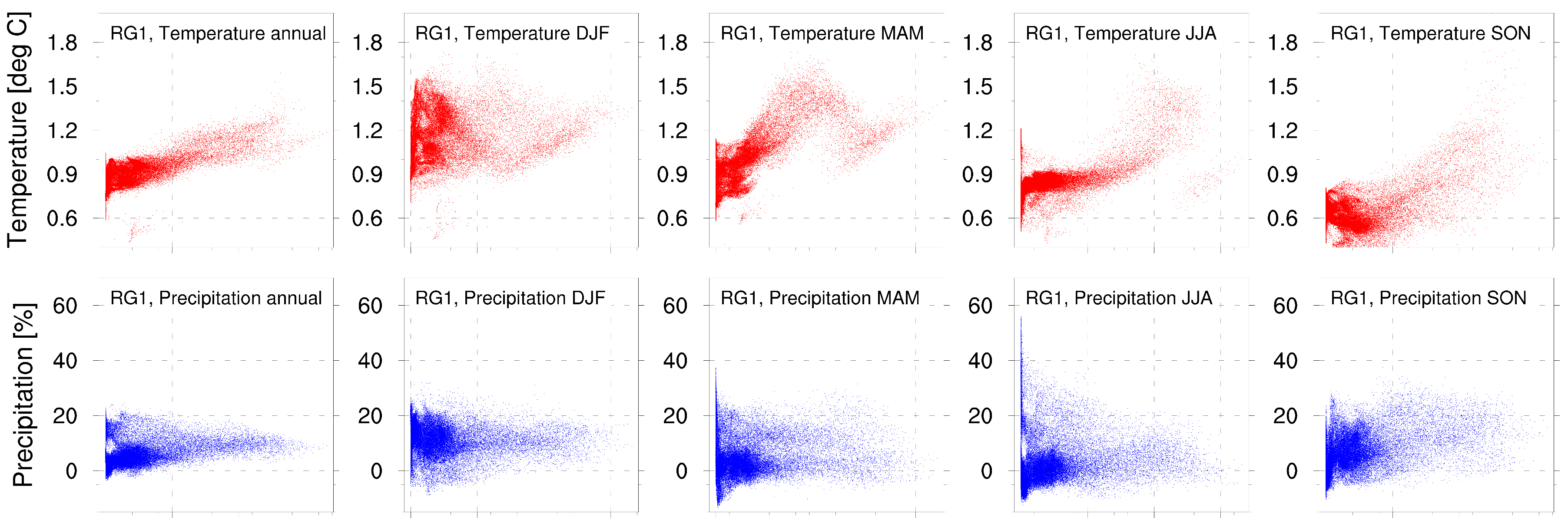
4.3.6. Elevation-Dependency of the Climate Change Signal

The high resolution of the presented WRF simulation allows an investigation of elevation-dependent effects in the climate change signal for the investigated region; 5 km or less and the implementation of non-hydrostatic equations for the atmosphere are a prerequisite for the effect to be captured [11,21,55]. Temperature and precipitation are key variables of particular relevance for climate impact analysis and are therefore assessed in the following. Elevation-dependent warming (EDW) results in accelerating change of mountain ecosystems, the cryosphere, the hydrological regimes and the biodiversity in the higher regions. Many evidences have been collected and documented in the recent past that the rate of climate change induced temperature increase is amplified in high altitudes, i.e., in the mountain regions of the world [20,22]. This evidence consists of both station recordings and model simulations (see Pepin et al. [21] for a review). The most striking example for EDW has been found for 139 stations on and around the Tibetan Plateau [56]. Generally, it is noticeable that the effect is more significant for minimum than for maximum temperatures, it may be limited to a certain elevation range, and both interdecadal and regional variabilities exist [21]. For the Swiss and Austrian Alps, e.g., the trends in the mountain station temperatures were higher than at the corresponding valley site by 0.36 °C per decade (Säntis/St. Gallen, 1971–2011), 0.17 °C per decade (Sonnblick/Bad Gastein, 1980–2011) and 0.13 °C per decade (Jungfraujoch/Interlaken, 1970–2011). The seasons with these maximum gradients were summer, spring, and winter, respectively [20]. This shows the high variability in the elevation-dependency of temperature trends, even in a period of general strong warming.
There are several mechanisms accounting for the phenomenon of EDW, similar to the ones explaining the latitudinal amplification of the warming rates [21]: first and probably most important, (i) the snow-albedo feedback around the mean elevation of the snowline causing a decrease in snow cover duration, which in turn leads to enhanced absorption of solar radiation, resulting in higher near-surface temperature. This effect can be amplified by the deposition of dark particles. Second, (ii) the temperature sensitivity to radiative forcing is higher for low temperatures. Third, (iii) long-wave radiation non-linearly depends on specific humidity such that an increase in the latter has a disproportionally large warming effect in drier conditions typical for higher elevations. Further, (iv) increased release of latent heat above the condensation level of a warmer and moister atmosphere results in additional warming in the respective elevation. The cooling effect of aerosols, on the other hand, is reduced in the higher elevations (v). The combinations of these mechanisms and changes in cloud cover and soil moisture, or the interannual to decadal variability of large-scale circulation patterns can lead to regional differences in the resulting EDW or they can even compensate for themselves.
The elevation-dependency of temperature and precipitation change in RG1, RG2, and RG3 for annual and seasonal differences is shown in Figure 19 by displaying the single change signal of the grid cells against the respective elevation. On annual average scale, an increase in warming is discernable in RG1, and RG2, ranging from approx. +0.9 °C to +1.2 °C for regions higher than 1500 m ASL. There is no such dependency in RG3. Investigating the seasonal distribution, the increase of warming with elevation in RG1 and RG2 is found in all seasons apart from winter (DJF). The dependency is the strongest in spring (MAM), rising from +0.9 °C in the low elevations to +1.5 °C in regions of 1000 to 1300 m ASL. However, when inspecting the values in regions higher than 1500 m ASL, there is a less pronounced second gradient from 1500 m ASL to 3000 m ASL. This particular effect can be located in Figure 14 (MAM), where a distinct band is present along the main Alpine Ridge with lower warming than the northern and southern adjacent regions, and including an isolated elevation gradient. A similar spatial feature is found in the winter months (DJF). There is no clear elevation-dependency for values lower than 1200 m ASL, and the warming signal strongly varies within these low elevations (from +0.9 °C to +1.5 °C) in this season. An increase in warming with elevation is found in regions higher than 1200 m ASL. Figure 14 reveals that this effect is produced by a distinct spatial pattern of the elevation-dependency. The warming signal is relatively high in the low elevated northeastern parts of RG1 with a general W-E gradient, which is overlayed by a negative warming gradient in the Northern Alps, whereas the gradient reverses at the main Alpine ridge to a positive one in the Southern Alps. These effects are reflected by the results for RG3. The region is limited to elevations up to 2000 m ASL in the 5 km WRF elevation model, and is located in the Northern Alps. The distinct increase of warming with elevation is seen in spring, and in the highest elevations in summer. In the spring months, there is a slight decreasing warming for elevations higher than 1500 m ASL. The winter months clearly show the above mentioned negative warming gradient with elevation. The general differences in seasonal changes discussed above can also be depicted in Figure 19, e.g., the warming signal in MAM being significantly higher (approx. +1.4 °C) compared to the SON signal (approx. +0.6 °C). Kotlarski et al. [57] and Gobiet et al. [7] found an increase of warming with higher elevations, whereas Smiatek et al. [8] could find such a dependency only for single simulations. As stated above and by Rangwala and Miller [58], and Winter et al. [55], the main cause for EDW is probably a positive feedback due to shortened snow cover durations in higher elevation, and the corresponding snow-albedo feedback. With the 5 km resolution of the simulations presented in this study it is possible to resolve this feedback system which might be an explanation for finding the elevation-dependency in temperature quite clearly. This additionally underlines the need for finer resolutions in RCM scenario simulations.
For precipitation changes, the patterns are more differentiated. In RG1, and RG2, an elevation-dependency is solely identifiable for the minimum annual and fall precipitation change showing increasing changes with higher elevations. The minimum change level increases from no change to an increase of +5% to +10% in the highest elevations. While lower resolved models generally show a decrease in summer precipitation over the Alps [8] an increase in high elevations was also found by Giorgi et al. [10] who attribute it to an increase in convective rainfall. A reversed relation is found only for JJA precipitation in RG3 where changes are between +5% in the lower elevations and −5% in the highest elevations. Apart from these effects, no clear elevation-dependency in precipitation change can be found in RG1, RG2, and RG3. The absent elevation-dependency for precipitation change in the Alps was also stated by Gobiet et al. [7] for the ENSEMBLES simulations, as well as by Smiatek et al. [8] for the EURO-CORDEX ensemble.

4.3.7. Precipitation Intensities

A possible change in precipitation intensities at different time scales is investigated by a comparison of probability density functions (PDF) of precipitation intensities for intervals of 1, 3, 5, and 10 days between the scenario 2020–2049 and control run 1980–2009 (Figure 20). To obtain comparable results for the regions and aggregation time scales, the PDFs are calculated using 20 bins for each value range which results in differently sized classes for the precipitation intensities. The respective bin spacing for the domains and time aggregation scales are listed in the caption of Figure 20. As described in Section 4.1, precipitation intensities <0.1 mm/d have been removed from the control and scenario to avoid overrepresentation of very small intensities that occur when averaging over a large region. Comparing the shape of the PDFs between the three regions RG1, RG2, and RG3, there are distinct differences. The smaller the regions is—RG3 (Figure 20, fifth and bottom row) being the smallest—the sharper and higher maximums occur for smaller precipitation intensities. This effect only reflects the methodical approach of areal aggregation and averaging over differently sized regions. It is evident by visual inspection of the paired black curves (control and scenario simulation) that the change signal in the PDFs is very small. However, when subtracting the two PDFs (difference plots with positive values in blue and negative values in red), there is still a clear signal. The positive changes are found at the larger intensities levels for all time scales. This means that the general increase in precipitation amounts is composed by an increased probability of higher precipitation intensities, outweighing the occurring decrease of small intensities (red indicated values). Jacob et al. [9] found the same effect in the EURO-CORDEX ensemble for daily intensities over Europe. A statistically significant increase in heavy precipitation in RCM scenario projections in Central Europe and the Alps was also reported by Knist et al. [17], Rajczak et al. [59], and Frei et al. [50].

5. Summary and Conclusions

Regional climate simulations at a very high, close to convection-permitting resolution of 5 km at a climate time scale are conducted and validated for large parts of Central Europe, the Alps, and a high Alpine region in the German Alps using both, gridded observation datasets, as well as station data. Focus of the study are the meteorological variables temperature, precipitation, relative humidity, incoming short-wave radiation, and wind speed, which are most commonly used in impact studies. The climate change signal for these variables is analysed in detail by comparing differences in seasonal, spatial and elevation-dependent distributions between the control period 1980–2009 and the near future scenario simulation 2020–2049. The future simulation is based on IPCC scenario RCP4.5. The presented analyses are limited to only one RCM simulation for one single RCP scenario. Other than for the decades after 2050, both the different RCP emission scenarios, as well as the corresponding projected climate change signals don’t differ largely for the considered period 2020–2049. However, the shown analyses are an exemplarily high-resolution climate change study only, but are instead comprehensive with respect to the regional, seasonal and elevation-dependent signal, and include the most important meteorological variables.
The reanalysis simulation reveals a very good performance in reproducing temperature for all investigated regions and scales. Averaged over the Alps, the mean bias in temperature is approx. −0.3 °C. The mean annual cycle is reproduced, and temporal dynamics are captured, even when comparing results for hourly data with observations at single stations. A precipitation bias in the simulation is found over the Alps which is in the typical range of current RCM simulations (e.g., the EURO-CORDEX ensemble simulations) when comparing them to gridded observation datasets. However, the bias is shown to be smaller in RG3 when comparing the model results to station data. Here, the bias is well within the typical observation uncertainties that are attributed to precipitation recordings in Alpine regions. The results for the validation of modeled incoming short-wave radiation at the station scale reveal a good model performance, whereas results for relative humidity and wind speed vary in their accuracy, depending on the station location and the respective terrain characteristics.
For the climate change signals between the period 1980–2009 and 2020–2049 (RCP4.5), different spatial and seasonal distributions for temperature and precipitation change are found, which strengthen the findings of Smiatek et al. [8], and Jacob et al. [9]. Beyond that, the presented 5 km resolution refines the findings, e.g., for particular seasonal and small-scale regional effects, as well as for elevation-dependencies. Additional regional patterns of changes in humidity, wind speed and short-wave radiation are found. The change in these meteorological variables are rarely assessed in current RCM studies, which are usually limited to temperature and precipitation changes. The mean warming in Central Europe is shown to vary between 0.44 °C and 1.59 °C with a spatial average of 0.90 °C (between 0.44 °C and 1.59 °C, on average 0.96 °C in the Alps/between 0.93 °C and 1.05 °C, on average 0.99 °C in the Berchtesgaden Alps). The strongest increase in temperature is found during winter and spring seasons, whereas warming is less distinct in summer and fall (from 0.33 °C to 0.80 °C less warming in fall than in spring season). An increase in warming with elevation is found in different specific regions and seasons but is absent in others and the gradient can even change its sign. Annual precipitation is shown to change between −4% and +25% in Central Europe with an average of +6% (Alps: between ±0% and +24%, on average +10%/Berchtesgaden Alps: between +4% and +13%, on average +8%) with distinct differences in seasonal changes. In the Central and Northern Alps, the increase in annual precipitation is mainly composed of a strong increase in fall and winter precipitation at all elevation levels, whereas spring and summer precipitation is almost unchanged. Precipitation intensities show a decrease in weak intensities with an increase in strong intensities in all investigated regions. The change signal for humidity, wind speed, and short-wave radiation are small, but distinct spatial and elevation-dependent patterns are found.
The presented work aims to complement the RCM ensemble simulation efforts, e.g., the EURO-CORDEX project for Europe [9] with a high-resolution simulation for Central Europe and the Alps. A detailed validation for varied spatial and temporal scales for different meteorological target variables is performed. It cannot be concluded from the presented results that the 5 km simulation is able to reduce RCM model biases or outperform the EURO-CORDEX simulations on temporal and spatial averages. However, the validation results show the benefits of the high spatial resolution. It facilitates a direct model validation at the station scale showing mostly good results and valuable insights, despite the 5 km grid size still being too coarse to reliably represent all terrain characteristics, which affect the microclimate in Alpine regions (e.g., very small-scale mountain-valley systems, absolute peak elevations, and the respective slope gradients). Specific processes that need to be parameterized or explicitly resolved by higher resolution simulations are e.g., small- and micro-scale slope flow and wind systems, or solar surface heating that impacts diurnal cycles. These are critical to energy and mass exchange in steep terrain, and particularly impact snow-albedo feedbacks and local convection enhancement. That said, the 5 km resolution of the simulations nevertheless enables to resolve many small spatial scale features and peculiarities as the local scale and the regional scale validation with high-resolution gridded observation datasets, as well as the differentiated change signal analysis over the Alps reveal. At the moment, the spatial resolution of 5 km bridges the gap between long-term, lower resolved RCM ensembles, and single, higher-resolution (convection-permitting), but shorter-term RCM simulations. This represents the current state-of-the-art until convection-permitting, long-term RCM simulations at continental scale will be feasible. The findings in the climate change signal strengthens recent results from the EURO-CORDEX project and contributes to further refine them for regional and local climate change studies such as the presented analysis of elevation-dependencies.

Author Contributions

Conceptualization, M.W. and H.K.; methodology, H.K., S.W. and M.W.; software, M.W. and S.W.; validation, M.W. and G.S.; formal analysis, M.W.; investigation, M.W., H.K., G.S.; data curation, M.W., G.S. and S.W.; writing–original draft preparation, M.W., H.K. and U.S.; writing–review and editing, P.L. and T.M.; visualization, M.W.; supervision, H.K. and U.S.; project administration, H.K., U.S., P.L. and M.W.; funding acquisition, H.K. and U.S.

Funding

This study received generous funding from the Bavarian State Ministry of the Environment and Consumer Protection (StMUV TKP01KPB-66747, BIASII), and from the German Ministry of Education and Research (BMBF, SYNOPSE).

Acknowledgments

The authors gratefully acknowledge the work of the WRF modeling community, the European Centre for Medium-Range Weather Forecast for the reanalysis data ERA-Interim, the MPI-M group for the CMIP5 data, the ECA&D group for the E-OBS data set, the ZAMG for the HISTALP and additional station data, MeteoSuisse for the EURO4M-APGD data, the Berchtesgaden National Park Administration for station data, and the Steinbuch Centre for Computing (SCC) of KIT for the possibility and their support to conduct the high-resolution RCM simulations on the HPC ForHLR1. The data are available at http://doi.org/10.5281/zenodo. 2533904.

Conflicts of Interest

The authors declare no conflict of interest. The funders had no role in the design of the study; in the collection, analyses, or interpretation of data; in the writing of the manuscript, or in the decision to publish the results.

References

  1. Pörtner, H.O.; Roberts, D.; Masson-Delmotte, V.; Zhai, P.; Tignor, M.; Poloczanska, E.; Mintenbeck, K.; Nicolai, M.; Okem, A.; Petzold, J.; et al. IPCC Special Report on the Ocean and Cryosphere in a Changing Climate; IPCC Intergovernmental Panel on Climate Change: Geneva, Switzerland, 2019. [Google Scholar]
  2. Beniston, M.; Farinotti, D.; Stoffel, M.; Andreassen, L.M.; Coppola, E.; Eckert, N.; Fantini, A.; Giacona, F.; Hauck, C.; Huss, M.; et al. The European mountain cryosphere: A review of its current state, trends, and future challenges. Cryosphere 2018, 12, 759–794. [Google Scholar] [CrossRef]
  3. Christensen, J.H.; Christensen, O.B. A summary of the PRUDENCE model projections of changes in European climate by the end of this century. Clim. Chang. 2007, 81, 7–30. [Google Scholar] [CrossRef]
  4. Van der Linden, P.; Mitchell, J.E. ENSEMBLES: Climate Change and Its Impacts—Summary of Research and Results from the ENSEMBLES Project; Met Office Hadley Centre: Exeter, UK, 2009; p. 160.
  5. Jacob, D.; Bärring, L.; Christensen, O.B.; Christensen, J.H.; de Castro, M.; Déqué, M.; Giorgi, F.; Hagemann, S.; Hirschi, M.; Jones, R.; et al. An inter-comparison of regional climate models for Europe: Model performance in present-day climate. Clim. Chang. 2007, 81, 31–52. [Google Scholar] [CrossRef]
  6. Kotlarski, S.; Keuler, K.; Christensen, O.B.; Colette, A.; Déqué, M.; Gobiet, A.; Goergen, K.; Jacob, D.; Lüthi, D.; van Meijgaard, E.; et al. Regional climate modeling on European scales: A joint standard evaluation of the EURO-CORDEX RCM ensemble. Geosci. Model Dev. 2014, 7, 1297–1333. [Google Scholar] [CrossRef]
  7. Gobiet, A.; Kotlarski, S.; Beniston, M.; Heinrich, G.; Rajczak, J.; Stoffel, M. 21st century climate change in the European Alps—A review. Sci. Total Environ. 2014, 493, 1138–1151. [Google Scholar] [CrossRef]
  8. Smiatek, G.; Kunstmann, H.; Senatore, A. EURO-CORDEX regional climate model analysis for the Greater Alpine Region: Performance and expected future change. J. Geophys. Res. Atmos. 2016, 121, 7710–7728. [Google Scholar] [CrossRef]
  9. Jacob, D.; Petersen, J.; Eggert, B.; Alias, A.; Christensen, O.B.; Bouwer, L.M.; Braun, A.; Colette, A.; Déqué, M.; Georgievski, G.; et al. EURO-CORDEX: New high-resolution climate change projections for European impact research. Reg. Environ. Chang. 2014, 14, 563–578. [Google Scholar] [CrossRef]
  10. Giorgi, F.; Torma, C.; Coppola, E.; Ban, N.; Schär, C.; Somot, S. Enhanced summer convective rainfall at Alpine high elevations in response to climate warming. Nat. Geosci. 2016, 9, 584. [Google Scholar] [CrossRef]
  11. Rasmussen, R.; Liu, C.; Ikeda, K.; Gochis, D.; Yates, D.; Chen, F.; Tewari, M.; Barlage, M.; Dudhia, J.; Yu, W.; et al. High-resolution coupled climate runoff simulations of seasonal snowfall over Colorado: A process study of current and warmer climate. J. Clim. 2011, 24, 3015–3048. [Google Scholar] [CrossRef]
  12. Zekollari, H.; Huss, M.; Farinotti, D. Modelling the future evolution of glaciers in the European Alps under the EURO-CORDEX RCM ensemble. Cryosphere 2019, 13, 1125–1146. [Google Scholar] [CrossRef] [Green Version]
  13. Prein, A.F.; Gobiet, A.; Truhetz, H.; Keuler, K.; Goergen, K.; Teichmann, C.; Fox Maule, C.; van Meijgaard, E.; Déqué, M.; Nikulin, G.; et al. Precipitation in the EURO-CORDEX 0.11° and 0.44° simulations: High resolution, high benefits? Clim. Dyn. 2016, 46, 383–412. [Google Scholar] [CrossRef]
  14. Ban, N.; Schmidli, J.; Schär, C. Evaluation of the convection-resolving regional climate modeling approach in decade-long simulations. J. Geophys. Res. Atmos. 2014, 119, 7889–7907. [Google Scholar] [CrossRef]
  15. Leutwyler, D.; Lüthi, D.; Ban, N.; Fuhrer, O.; Schär, C. Evaluation of the convection-resolving climate modeling approach on continental scales. J. Geophys. Res. Atmos. 2017, 122, 5237–5258. [Google Scholar] [CrossRef]
  16. Coppola, E.; Sobolowski, S.; Pichelli, E.; Raffaele, F.; Ahrens, B.; Anders, I.; Ban, N.; Bastin, S.; Belda, M.; Belusic, D.; et al. A first-of-its-kind multi-model convection permitting ensemble for investigating convective phenomena over Europe and the Mediterranean. Clim. Dyn. 2018, 1–32. [Google Scholar] [CrossRef]
  17. Knist, S.; Goergen, K.; Simmer, C. Evaluation and projected changes of precipitation statistics in convection-permitting WRF climate simulations over Central Europe. Clim. Dyn. 2018, 1–17. [Google Scholar] [CrossRef]
  18. Kendon, E.J.; Stratton, R.A.; Tucker, S.; Marsham, J.H.; Berthou, S.; Rowell, D.P.; Senior, C.A. Enhanced future changes in wet and dry extremes over Africa at convection-permitting scale. Nat. Commun. 2019, 10, 1794. [Google Scholar] [CrossRef]
  19. Prein, A.F.; Langhans, W.; Fosser, G.; Ferrone, A.; Ban, N.; Goergen, K.; Keller, M.; Tölle, M.; Gutjahr, O.; Feser, F.; et al. A review on regional convection-permitting climate modeling: Demonstrations, prospects, and challenges. Rev. Geophys. 2015, 53, 323–361. [Google Scholar] [CrossRef]
  20. Ohmura, A. Enhanced temperature variability in high-altitude climate change. Theor. Appl. Climatol. 2012, 110, 499–508. [Google Scholar] [CrossRef]
  21. Pepin, N.; Bradley, R.; Diaz, H.; Baraer, M.; Caceres, E.; Forsythe, N.; Fowler, H.; Greenwood, G.; Hashmi, M.; Liu, X.; et al. Elevation-dependent warming in mountain regions of the world. Nat. Clim. Chang. 2015, 5, 424–430. [Google Scholar] [Green Version]
  22. Wang, Q.; Wang, M.; Fan, X. Seasonal patterns of warming amplification of high-elevation stations across the globe. Int. J. Climatol. 2018, 38, 3466–3473. [Google Scholar] [CrossRef]
  23. Haylock, M.; Hofstra, N.; Klein Tank, A.; Klok, E.; Jones, P.; New, M. A European daily high-resolution gridded dataset of surface temperature and precipitation for 1950–2006. J. Geophys. Res. 2008, 113, 2156–2202. [Google Scholar] [CrossRef]
  24. Van den Besselaar, E.; Haylock, M.; van der Schrier, G.; Klein Tank, A. A European daily high-resolution observational gridded data set of sea level pressure. J. Geophys. Res. 2011, 116, 1–11. [Google Scholar] [CrossRef]
  25. Efthymiadis, D.; Jones, P.; Briffa, K.; Auer, I.; Böhm, R.; Schöner, W.; Frei, C.; Schmidli, J. Construction of a 10-min-gridded precipitation data set for the Greater Alpine Region for 1800-2003. J. Geophys. Res. 2006, 111. [Google Scholar] [CrossRef]
  26. Hiebl, J.; Auer, I.; Böhm, R.; Schöner, W.; Maugeri, M.; Lentini, G.; Spinoni, J.; Brunett, M.; Nanni, T.; Tadi’c, M.P.; et al. A high-resolution 1961–1990 monthly temperature climatology for the greater Alpine region. Meteorol. Z. 2009, 18, 507–530. [Google Scholar] [CrossRef]
  27. Isotta, F.; Frei, C.; Weilguni, V.; Perčec Tadić, M.; Lassègues, P.; Rudolf, B.; Pavan, V.; Cacciamani, C.; Antolini, G.; Ratto, S.; et al. The climate of daily precipitation in the Alps: Development and analysis of a high-resolution grid dataset from pan-Alpine rain-gauge data. Int. J. Climatol. 2014, 34, 1657–1675. [Google Scholar] [CrossRef]
  28. Skamarock, W.; Klemp, J.; Dudhia, J.; Gill, D.; Barker, D.; Duda, M.; Huang, X.; Wang, W.; Powers, J. A Description of the Advanced Research WRF Version 3; Technical Reports NCAR/TN-475+STR, NCAR TECHNICAL NOTE; University Corporation for Atmospheric Research: Boulder, CO, USA, 2008; p. 113. [Google Scholar]
  29. Hong, S.; Lim, J. The WRF Single-Moment 6-Class Microphysics Scheme (WSM6). J. Korean Meteorol. Soc. 1990, 42, 129–151. [Google Scholar]
  30. Grell, G.A.; Freitas, S.R. A scale and aerosol aware stochastic convective parameterization for weather and air quality modeling. Atmos. Chem. Phys. 2014, 14, 5233–5250. [Google Scholar] [CrossRef] [Green Version]
  31. Chen, F.; Dudhia, J. Coupling an Advanced Land Surface-Hydrology Model with the Penn State-NCAR MM5 Modeling System. Part I: Model Implementation and Sensitivity. Mon. Weather Rev. 2001, 129, 569–585. [Google Scholar] [CrossRef]
  32. Chen, F.; Dudhia, J. Coupling an Advanced Land Surface-Hydrology Model with the Penn State-NCAR MM5 Modeling System. Part II: Preliminary Model Validation. Mon. Weather Rev. 2001, 129, 587–604. [Google Scholar] [CrossRef]
  33. Hong, S.; Noh, Y.; Dudhia, J. A new vertical diffusion package with an explicit treatment of entrainment processes. Mon. Weather Rev. 2006, 134, 2318–2341. [Google Scholar] [CrossRef]
  34. Iacano, M.; Delamere, J.; Mlawer, E.; Shephard, M.; Clough, S.; Collins, W. Radiative forcing by long-lived greenhouse gases: Calculations with the AER radiative transfer models. J. Atmos. Sci. 2008, 113. [Google Scholar] [CrossRef]
  35. Katragkou, E.; García-Díez, M.; Vautard, R.; Sobolowski, S.; Zanis, P.; Alexandri, G.; Cardoso, R.M.; Colette, A.; Fernandez, J.; Gobiet, A.; et al. Regional climate hindcast simulations within EURO-CORDEX: Evaluation of a WRF multi-physics ensemble. Geosci. Model Dev. 2015, 8, 603–618. [Google Scholar] [CrossRef]
  36. García-Díez, M.; Fernández, J.; Vautard, R. An RCM multi-physics ensemble over Europe: Multi-variable evaluation to avoid error compensation. Clim. Dyn. 2015, 45, 3141–3156. [Google Scholar] [CrossRef]
  37. Wagner, A.; Heinzeller, D.; Wagner, S.; Rummler, T.; Kunstmann, H. Explicit Convection and Scale-Aware Cumulus Parameterizations: High-Resolution Simulations over Areas of Different Topography in Germany. Mon. Weather Rev. 2018, 146, 1925–1944. [Google Scholar] [CrossRef]
  38. Warscher, M. High-Resolution (5 km) RCM data for Central Europe, 1980–2009 and 2020-2049, WRF 3.6.1 forced by ERA-Interim and MPI-ESM, RCP4.5. 2019. Available online: https://doi.org/10.5281/zenodo.2533904 (accessed on 1 November 2019).
  39. Dee, D.P.; Uppala, S.M.; Simmons, A.J.; Berrisford, P.; Poli, P.; Kobayashi, S.; Andrae, U.; Balmaseda, M.A.; Balsamo, G.; Bauer, P.; et al. The ERA-Interim reanalysis: Configuration and performance of the data assimilation system. Q. J. R. Meteorol. Soc. 2011, 137, 553–597. [Google Scholar] [CrossRef]
  40. Giorgetta, M.; Jungclaus, J.; Reick, C.; Legutke, S.; Brovkin, V.; Crueger, T.; Esch, M.; Fieg, K.; Glushak, K.; Gayler, V.; et al. CMIP5 Simulations of the Max Planck Institute for Meteorology (MPI-M) Based on the MPI-ESM-LR Model: The rcp45 Experiment, Served by ESGF. 2012. Available online: https://doi.org/10.1594/WDCC/CMIP5.MXELr4 (accessed on 1 November 2019).
  41. Stevens, B.; Giorgetta, M.; Esch, M.; Mauritsen, T.; Crueger, T.; Rast, S.; Salzmann, M.; Schmidt, H.; Bader, J.; Block, K.; et al. Atmospheric component of the MPI-M Earth System Model: ECHAM6. J. Adv. Model Earth Syst. 2013, 5, 146–172. [Google Scholar] [CrossRef]
  42. Van Vuuren, D.P.; Edmonds, J.; Kainuma, M.; Riahi, K.; Thomson, A.; Hibbard, K.; Hurtt, G.C.; Kram, T.; Krey, V.; Lamarque, J.F.; et al. The representative concentration pathways: an overview. Clim. Chang. 2011, 109, 5–31. [Google Scholar] [CrossRef]
  43. Marke, T.; Strasser, U.; Kraller, G.; Warscher, M.; Kunstmann, H.; Franz, H.; Vogel, M. The Berchtesgaden National Park (Bavaria, Germany): A platform for interdisciplinary catchment research. Environ. Earth Sci. 2013, 69, 679–694. [Google Scholar] [CrossRef]
  44. Warscher, M.; Strasser, U.; Kraller, G.; Marke, T.; Franz, H.; Kunstmann, H. Performance of complex snow cover descriptions in a distributed hydrological model system: A case study for the high Alpine terrain of the Berchtesgaden Alps. Water Resour. Res. 2013, 49, 2619–2637. [Google Scholar] [CrossRef] [Green Version]
  45. Warrach-Sagi, K.; Schwitalla, T.; Wulfmeyer, V.; Bauer, H. Evaluation of a climate simulation in Europe based on the WRF-NOAH model system: Precipitation in Germany. Clim. Dyn. 2013, 41, 755–774. [Google Scholar] [CrossRef]
  46. Kotlarski, S.; Szabó, P.; Herrera, S.; Räty, O.; Keuler, K.; Soares, P.M.; Cardoso, R.M.; Bosshard, T.; Pagé, C.; Boberg, F.; et al. Observational uncertainty and regional climate model evaluation: A pan-European perspective. Int. J. Climatol. 2017, 39. [Google Scholar] [CrossRef]
  47. Frei, C.; Christensen, J.H.; Déqué, M.; Jacob, D.; Jones, R.G.; Vidale, P.L. Daily precipitation statistics in regional climate models: Evaluation and intercomparison for the European Alps. J. Geophys. Res. Atmos. 2003, 108. [Google Scholar] [CrossRef]
  48. Prein, A.F.; Gobiet, A. Impacts of uncertainties in European gridded precipitation observations on regional climate analysis. Int. J. Climatol. 2017, 37, 305–327. [Google Scholar] [CrossRef] [PubMed]
  49. Pieri, A.; von Hardenberg, J.; Parodi, A.; Provenzale, A. Sensitivity of Precipitation Statistics to Resolution, Microphysics, and Convective Parameterization: A Case Study with the High-Resolution WRF Climate Model over Europe. J. Hydrometeorol. 2015, 16, 1857–1872. [Google Scholar] [CrossRef]
  50. Frei, C.; Schöll, R.; Fukutome, S.; Schmidli, J.; Vidale, P.L. Future change of precipitation extremes in Europe: Intercomparison of scenarios from regional climate models. J. Geophys. Res. Atmos. 2006, 111. [Google Scholar] [CrossRef] [Green Version]
  51. Pachauri, R.K.; Allen, M.R.; Barros, V.R.; Broome, J.; Cramer, W.; Christ, R.; Church, J.A.; Clarke, L.; Dahe, Q.; Dasgupta, P.; et al. (Eds.) Climate Change 2014: Synthesis Report. Contribution of Working Groups I, II and III to the Fifth Assessment Report of the Intergovernmental Panel on Climate Change; IPCC: Geneva, Switzerland, 2014; p. 151. [Google Scholar]
  52. Berg, P.; Wagner, S.; Kunstmann, H.; Schädler, G. High resolution regional climate model simulations for Germany: Part I—Validation. Clim. Dyn. 2013, 40, 401–414. [Google Scholar] [CrossRef]
  53. Wagner, S.; Berg, P.; Schädler, G.; Kunstmann, H. High resolution regional climate model simulations for Germany: Part II—Projected climate changes. Clim. Dyn. 2013, 40, 415–427. [Google Scholar] [CrossRef]
  54. Jerez, S.; Tobin, I.; Vautard, R.; Montávez, J.P.; López-Romero, J.M.; Thais, F.; Bartok, B.; Christensen, O.B.; Colette, A.; Déqué, M.; et al. The impact of climate change on photovoltaic power generation in Europe. Nat. Commun. 2015, 6, 10014. [Google Scholar] [CrossRef] [Green Version]
  55. Winter, K.; Kotlarski, S.; Scherrer, S.; Schär, C. The Alpine snow-albedo feedback in regional climate models. Clim. Dyn. 2017, 48, 1109–1124. [Google Scholar] [CrossRef]
  56. Yan, L.; Liu, X. Has climatic warming over the Tibetan Plateau paused or continued in recent years. J. Earth Ocean Atmos. Sci. 2014, 1, 13–28. [Google Scholar]
  57. Kotlarski, S.; Bosshard, T.; Lüthi, D.; Pall, P.; Schär, C. Elevation gradients of European climate change in the regional climate model COSMO-CLM. Clim. Chang. 2012, 112, 189–215. [Google Scholar] [CrossRef]
  58. Rangwala, I.; Miller, J.R. Climate change in mountains: A review of elevation-dependent warming and its possible causes. Clim. Chang. 2012, 114, 527–547. [Google Scholar] [CrossRef]
  59. Rajczak, J.; Pall, P.; Schär, C. Projections of extreme precipitation events in regional climate simulations for Europe and the Alpine Region. J. Geophys. Res. Atmos. 2013, 118, 3610–3626. [Google Scholar] [CrossRef]
Figure 1. WRF domain configuration and nesting strategy (top): Domain 1 (D1: 45 km), Domain 2 (D2: 15 km), and Domain 3 (D3: 5 km). The investigated regions (bottom left), and a closeup of RG3 and the 5 km WRF terrain model (bottom right) are displayed. The black boxes in the bottom left figure mark the three regions that are focus of the study: RG1 (parts of Central Europe, Germany and the Alps), RG2 (the Alps and its surroundings), and RG3 (the Berchtesgaden Alps in South-East Germany).
Atmosphere 10 00682 g001
Figure 2. Annual and seasonal temperature difference for the reanalysis simulation 1980–2009 compared to E-OBS data in RG1 (top row), and to HISTALP in RG2 (center row) and RG3 (bottom row), respectively.
Atmosphere 10 00682 g002
Figure 3. Mean annual cycle 1980–2009 of temperature for the reanalysis simulation and the observation datasets, and the monthly model bias averaged for RG1 (top), RG2 (center), and RG3 (bottom).
Atmosphere 10 00682 g003
Figure 4. Mean annual precipitation for the WRF reanalysis simulation 1980–2008 (left: D2, Δ x/ Δ y = 15 km, center: D3, Δ x/ Δ y = 5 km) and the respective EURO4M-APGD observation data (right) for RG2. The spatial pattern correlation between the two model resolutions and observed values is expressed as the centered Pearson product-moment coefficient of linear correlation (0.70 for WRF in the 15 km domain D2, and 0.82 in the 5 km domain D3).
Atmosphere 10 00682 g004
Figure 5. Annual and seasonal percentage difference in precipitation for the reanalysis simulation 1980–2009 compared to E-OBS data in RG1 (top row), to HISTALP (second row) in RG2, and to EURO4M-APGD (1980–2008) in RG2 (third row)/in RG3 (bottom row).
Atmosphere 10 00682 g005
Figure 6. Mean annual cycle 1980–2009 (1980–2008 for EURO4M-APGD/1989–2008 where EURO-CORDEX is shown) of precipitation for the simulations and the observation datasets, and the monthly model bias averaged over RG1 (top), RG2 (center), and RG3 (bottom).
Atmosphere 10 00682 g006
Figure 7. Probability density functions for precipitation intensities from the WRF simulation and from the E-OBS/EURO4M-APGD observation data for RG1 (top row), RG2 (center row), and RG3 (bottom row) in mm per 1 day/3 days/5 days/10 days (moving window, from left to right). The bin sizes for the PDFs are for RG1: 0.9, 2.0, 2.6, and 4.1 mm, for RG2: 1.8, 3.3, 4.6, and 6.9 mm, and for RG3: 3.8, 8.3, 9.9, and 12.0 mm.
Atmosphere 10 00682 g007
Figure 8. Elevation differences between WRF model grid cells and the corresponding measurement stations for the domains D2 (15 km) and D3 (5 km). The left figure shows scatter plots for the two domains, the right one displays the differences between model cell and station elevation depending on absolute elevation of the station.
Atmosphere 10 00682 g008
Figure 9. Temperature (left) and precipitation (right) modeled and measured at the station Loferer Alm (1623 m ASL) for the period 2001–2009. From top to bottom the panel shows hourly (top row), daily (center row), and monthly (bottom row) aggregated data.
Atmosphere 10 00682 g009
Figure 10. Scatter plot for temperature (top row) and precipitation (bottom row) modeled and measured at the station Loferer Alm (1623 m ASL) for the period 2001–2009. From left to right the panel shows hourly, daily, and monthly aggregated data.
Atmosphere 10 00682 g010
Figure 11. Relative humidity (left) and wind speed (right) modeled and measured at the station Loferer Alm (1623 m ASL) for the period 2001–2009. From top to bottom the panel shows hourly (top row), daily (center row), and monthly (bottom row) aggregated data.
Atmosphere 10 00682 g011
Figure 12. Incoming short-wave radiation modeled and measured at the station Loferer Alm (1623 m ASL) for the period 2001–2009. From top to bottom the panel shows hourly (top), daily (center), and monthly (bottom) aggregated data.
Atmosphere 10 00682 g012
Figure 13. Projected changes 2020–2049 (scenario RCP4.5) compared to 1980–2009 for mean annual temperature (top left), precipitation (top center and right), humidity (bottom left), wind speed (bottom center), and short-wave radiation (bottom right) based on the 5 km simulation (domain D3). The black boxes mark the three investigated regions.
Atmosphere 10 00682 g013
Figure 14. Projected changes 2020–2049 (scenario RCP4.5) compared to 1980–2009 for temperature for RG1, RG2 (top row), and RG3 (bottom row). Annual, winter (DJF), spring (MAM), summer (JJA), and fall (SON) changes are displayed (from left to right).
Atmosphere 10 00682 g014
Figure 15. Projected changes 2020–2049 (scenario RCP4.5) compared to 1980–2009 for precipitation over RG1, RG2 (top row), and RG3 (second row), as well as percentage precipitation change over RG1, RG2 (third row), and RG3 (bottom row). Annual, winter (DJF), spring (MAM), summer (JJA), and fall (SON) changes are displayed (from left to right).
Atmosphere 10 00682 g015
Figure 16. Projected changes 2020–2049 (scenario RCP4.5) compared to 1980–2009 for relative humidity for RG1, RG2 (top row), and RG3 (bottom row). Annual, winter (DJF), spring (MAM), summer (JJA), and fall (SON) changes are displayed (from left to right).
Atmosphere 10 00682 g016
Figure 17. Projected changes 2020–2049 (scenario RCP4.5) compared to 1980–2009 for wind speed for RG1, RG2 (top row), and RG3 (bottom row). Annual, winter (DJF), spring (MAM), summer (JJA), and fall (SON) changes are displayed (from left to right).
Atmosphere 10 00682 g017
Figure 18. Projected changes 2020–2049 (scenario RCP4.5) compared to 1980–2009 for incoming short-wave radiation over RG1, RG2 (top row), and RG3 (bottom row). Annual, winter (DJF), spring (MAM), summer (JJA), and fall (SON) changes are displayed (from left to right).
Atmosphere 10 00682 g018
Figure 19. Annual and seasonal elevation-dependency of projected changes (2020–2049 compared to 1980–2009) in temperature and precipitation for RG1 (first and second row), RG2 (third and fourth row), and RG3 (fifth and last row).
Atmosphere 10 00682 g019aAtmosphere 10 00682 g019b
Figure 20. Probability density functions (PDF) of precipitation intensities for intervals of 1, 3, 5, and 10 days (moving window, from left to right) and the changes in the PDFs between the scenario (2020–2049) and control run (1980–2009) for RG1 (first and second row), RG2 (third and fourth row), and RG3 (fifth and last row). The bin sizes for the PDFs are for RG1: 1.2, 1.9, 2.7, and 4.6 mm, for RG2: 1.9, 3.8, 4.9, and 8.7 mm, and for RG3: 6.1, 15.3, 19.3, and 21.4 mm.
Atmosphere 10 00682 g020
Table 1. R 2 values for WRF (ERA-Interim) results against station data for the period 2001–2009 and the variables temperature, precipitation, humidity, wind speed, and short-wave radiation (hourly, daily, and monthly, g.c. = grid cell, st. = station, n.a. = not available).
StationElevationΔElevationTemperaturePrecipitationHumidityWind SpeedSW Radiation
m ASLm (g.c. - st.)hourdaymonthhourdaymonthhourdaymonthhourdaymonthhourdaymonth
Reiteralm 11753−7470.860.920.92n.a.n.a.n.a.0.530.690.610.270.480.42n.a.n.a.n.a.
Reiteralm 21679−6620.890.930.96n.a.n.a.n.a.0.500.660.46n.a.n.a.n.a.0.480.600.85
Reiteralm 31611−6070.900.960.95n.a.n.a.n.a.0.450.670.36n.a.n.a.n.a.0.540.750.90
Schoenau617+2810.800.900.970.060.440.740.060.200.050.020.150.000.540.760.96
Jenner 11219+3100.840.910.97n.a.n.a.n.a.0.410.570.40n.a.n.a.n.a.n.a.n.a.n.a.
Hoellgraben640+4630.690.790.900.060.470.690.090.210.15n.a.n.a.n.a.n.a.n.a.n.a.
Kuehroint1407−2150.900.950.970.050.360.480.530.710.580.080.140.050.560.710.91
Funtenseetauern2522−5390.770.830.89n.a.n.a.n.a.0.470.640.520.120.160.11n.a.n.a.n.a.
Hinterberghorn2270−6510.800.860.71n.a.n.a.n.a.0.320.450.290.090.140.120.510.500.91
Schlunghorn2155−6450.820.92n.a.n.a.n.a.n.a.0.410.61n.a.0.330.56n.a.n.a.n.a.n.a.
Watzmannhaus1919−7270.880.940.97n.a.n.a.n.a.0.530.700.670.320.560.800.570.690.86
Blaueis1651−619n.a.n.a.n.a.n.a.n.a.n.a.0.510.660.51n.a.n.a.n.a.n.a.n.a.n.a.
Hinterseeau839+7150.780.910.98n.a.n.a.n.a.n.a.n.a.n.a.n.a.n.a.n.a.0.500.690.96
Brunftbergtiefe1238+1130.830.880.960.070.440.85n.a.n.a.n.a.n.a.n.a.n.a.0.500.660.85
Lofer625+4290.870.920.970.090.500.650.180.290.05n.a.n.a.n.a.0.740.760.95
Loferer Alm1623−4040.870.930.980.090.470.560.510.700.570.280.570.770.750.730.88
Salzburg Flughafen430−400.910.950.99n.a.n.a.n.a.0.260.400.450.140.390.51n.a.n.a.n.a.
Schmittenhoehe1973−747n.a.n.a.n.a.0.070.430.650.500.690.520.090.210.050.720.670.95
Golling491+2720.910.950.960.100.430.670.340.560.520.030.040.090.750.790.95
Saalbach974+4810.830.890.970.080.420.49n.a.n.a.n.a.0.030.140.230.730.810.95
Average1382−1770.840.910.940.070.440.640.390.550.420.150.300.290.610.700.91
Table 2. RMSE values for WRF (ERA-Interim) results against station data for the period 2001–2009 and the variables temperature, precipitation, humidity, wind speed, and short-wave radiation (hourly, daily, and monthly) and percentage bias (PBias) for precipitation (g.c. = grid cell, st. = station, n.a. = not available).
StationElevationΔElevationTemperaturePrecipitationHumidityWind SpeedSW Radiation
m ASLm °C mm % % m/s W/m2
g.c. - st.hourdaymonthhourdaymonthPBiashourdaymonthhourdaymonthhourdaymonth
Reiteralm 11753−7473.112.321.94n.a.n.a.n.a.n.a.12.748.423.931.160.750.34n.a.n.a.n.a.
Reiteralm 21679−6622.772.061.39n.a.n.a.n.a.n.a.13.128.754.26n.a.n.a.n.a.186.1362.7331.71
Reiteralm 31611−6072.701.711.51n.a.n.a.n.a.n.a.13.948.804.38n.a.n.a.n.a.163.6146.4526.07
Schoenau617+2813.742.491.140.666.4149.62+2417.6913.305.371.210.820.35174.9847.8517.41
Jenner 11219+3103.342.431.25n.a.n.a.n.a.n.a.13.699.484.54n.a.n.a.n.a.n.a.n.a.n.a.
Jenner 2640+4634.453.442.240.768.5697.82+6318.0513.656.02n.a.n.a.n.a.n.a.n.a.n.a.
Kuehroint1407−2152.631.831.190.818.4294.19+5412.948.334.281.531.170.56167.6151.6124.59
Funtenseetauern2522−5394.153.352.42n.a.n.a.n.a.n.a.12.298.294.241.901.600.79n.a.n.a.n.a.
Hinterberghorn2270−6513.823.153.97n.a.n.a.n.a.n.a.14.4010.273.832.131.670.92176.0466.5823.73
Schlunghorn2155−6452.951.82n.a.n.a.. n.a.n.a.n.a.15.039.69n.a.1.761.05n.a.n.a.n.a.n.a.
Watzmannhaus1919−7272.811.921.09n.a.n.a.n.a.n.a.12.758.293.341.400.900.31155.4151.0829.37
Blaueis1651−619n.a.n.a.n.a.n.a.n.a.n.a.n.a.13.108.954.43n.a.n.a.n.a.n.a.n.a.n.a.
Hinterseeau839+7153.822.351.20n.a.n.a.n.a.n.a.n.a.n.a.n.a.n.a.n.a.n.a.186.4454.4516.61
Brunftbergtiefe1238+1133.682.911.610.899.2757.21+19n.a.n.a.n.a.n.a.n.a.n.a.179.5656.6933.72
Lofer625+4293.122.331.160.696.2155.32+1916.5412.135.31n.a.n.a.n.a.133.4647.0418.00
Loferer Alm1623−4043.072.201.060.777.2161.05+4112.517.673.541.030.610.21126.2949.8227.74
Salzburg Flugh.430−402.651.850.71n.a.n.a.n.a.n.a.14.4810.274.311.000.540.22n.a.n.a.n.a.
Schmittenhoehe1973−747n.a.n.a.n.a.0.585.1441.96−712.787.633.720.970.600.21136.3854.0418.12
Golling491+2722.611.801.500.646.0054.28+3615.1810.164.321.461.120.47122.4345.0219.81
Saalbach974+4813.632.731.290.716.7662.14+85n.a.n.a.n.a.1.501.120.53129.1440.8818.51
Average1382−1773.282.371.570.727.1163.73+3714.199.654.361.421.000.45156.7351.8623.49
Table 3. Areal minimum, maximum, and average differences between scenario and control run for the variables temperature, precipitation, humidity, wind speed, and short-wave radiation in the three investigated regions RG1, RG2, and RG3.
TemperaturePrecipitationHumidityWind speedSW radiation
K mm % % m/s W/m2
min.max.avg.min.max.avg.min.max.avg.min.max.avg.min.max.avg.min.max.avg.
RG1 ann.+0.44+1.59+0.90−40+666+83−4+25+6−3.37+1.61−0.20−0.22+0.25+0.06−8.31+0.72−1.91
    DJF+0.46+1.73+1.13−60+331+ 32−9+32+11−4.73+2.95−0.96−0.43+0.56+0.15−5.77+1.50−1.56
    MAM+0.42+1.73+0.97−55+215+16−13+37+5−4.53+1.79−0.22−0.30+0.47+0.17−18.94+0.90−3.40
    JJA+0.43+1.72+0.84−70+198+10−12+67+3−3.78+4.46+0.22−0.57+0.29−0.05−17.60+5.56−0.39
    SON+0.21+2.27+0.64−55+317+19−10+38+6−8.61+2.760−0.78+0.58+0.01−10.77+4.20−1.45
RG2 ann.+0.44+1.59+0.96+2+666+1550+24+10−3.37+1.61+0.03−0.22+0.250−8.31−0.73−2.94
    DJF+0.46+1.73+1.15−60+331+34−9+32+8−4.73+2.95−0.92−0.43+0.56+0.05−5.77+1.03−2.13
    MAM+0.56+1.73+1.11−55+215+35−10+37+9−4.53+1.79−0.33−0.30+0.45+0.05−18.94+0.85−4.56
    JJA+0.43+1.72+0.90−70+198+32−10+67+10−3.78+4.46+0.96−0.57+0.29−0.08−17.60+4.20−2.48
    SON+0.21+2.27+0.68−55+317+40−8+38+9−8.61+2.76−0.01−0.78+0.58−0.02−10.77+4.20−1.52
RG3 ann.+0.93+1.05+0.99+77+298+169+4+13+8−0.60+0.63+0.04−0.07+0.060−7.12−2.50−4.61
    DJF+0.88+1.31+1.04+22+121+59+6+27+13−2.38+1.86+0.43−0.10+0.23+0.03−4.22−1.16−2.69
    MAM+1.18+1.55+1.41−19+41+10−3+10+2−3.14−0.06−1.69−0.05+0.16+0.03−12.22−1.97−6.90
    JJA+0.80+1.13+0.89−39+540−5+80−1.12+0.95+0.46−0.17+0.03−0.06−11.28+0.24−2.65
    SON+0.42+0.74+0.61+48+173+99+16+33+23+0.18+2.76+0.86−0.30+0.18+0.02−8.04−1.83−5.87

