Parameterization of Wave Boundary Layer


1
Shirshov Institute of Oceanology, RAS, Saint-Petersburg 197110, Russia
2
Department of Infrastructure Engineering, Melbourne School of Engineering, University of Melbourne, Victoria 3010, Australia
3
Laboratory for Regional Oceanography and Numerical Modeling, National Laboratory for Marine Science and Technology, Qingdao 266237, China
*
Author to whom correspondence should be addressed.
Atmosphere 2019, 10(11), 686; https://doi.org/10.3390/atmos10110686
Submission received: 9 October 2019
/
Revised: 25 October 2019
/
Accepted: 2 November 2019
/
Published: 7 November 2019
(This article belongs to the Special Issue Wind-Wave Interaction)
Abstract
:It is known that drag coefficient varies in broad limits depending on wind velocity and wave age as well as on wave spectrum and some other parameters. All those effects produce large scatter of the drag coefficient, so, the data is plotted as a function of wind velocity forming a cloud of points with no distinct regularities. Such uncertainty can be overcome by the implementation of the WBL model instead of the calculations of drag with different formulas. The paper is devoted to the formulation of the Wave Boundary Layer (WBL) model for the parameterization of the ocean-atmosphere interactions in coupled ocean-atmosphere models and wave prediction models. The equations explicitly take into account the vertical flux of momentum generated by the wave-produced fluctuations of pressure, velocity and stresses (WPMF). Their surface values are calculated with the use of the spectral beta-functions whose expression was obtained by means of the 2-D simulation of the WBL. Hence, the model directly connects the properties of the WBL with an arbitrary wave spectrum. The spectral and direct wave modeling should also take into account the momentum flux to a subgrid part of the spectrum. The parameterization of this effect in the present paper is formulated in terms of wind and cut-off frequency of the spectrum.
1. Introduction
A theory of the surface layer for the case of the flat underlying surface is well developed and confirmed by experimental data. The Monin-Obukhov similarity theory for the stratified surface layer is used in all atmospheric models. The lowest layer of such numerical model is usually identified as the surface layer. It is supposed that the surface layer is close to the state of local horizontal homogeneity and stationarity and, consequently, the vertical divergence of momentum, energy and vapor is equal to zero. It means that the vertical fluxes remain constant by height. As a rule, in the lowest layer all other terms of equations are also taken into account, but their influence is small, so, the vertical structure of layer can be described with the Monin-Obukhov similarity theory. Above the surface layer up to the height of the order of one kilometer, extends the atmospheric boundary layer. Attempts were also made to parameterize the effects of this layer (which is often called the ‘Ekman layer’), but generally with no success. This was because in contrast to the surface layer, all terms of the equations, including the Corioles force, are of the same order of value. Hence, the structure of the Ekman layer cannot be in the least degree universal. The so called Ekman layer turns out to be more complicated than ‘free atmosphere’ because of the strong influence of the vertical turbulent fluxes produced by velocity shear and convective motions.
The surface layer above the sea is generally similar to the surface layer above a solid surface, so for the calculation of fluxes, the same methods are usually accepted. However, there is a significant difference in the presence of a moving and curvilinear lower boundary. The most popular way to take this property into account is the introduction of the Charnock relation for the roughness parameter of sea surface :
where is the friction velocity ( is a vector of the vertical kinematic momentum flux at the upper level of surface layer); is an empirical coefficient of the order of 0.01, g is the gravity acceleration. The length scale was introduced in a famous one-page paper by Charnock [1]. This scale always appears in a theory of wind-wave interaction, so it is reasonable to call it the ‘Charnock scale’. Formula (1) can be used for estimation of the drag coefficient at height
where is von Karman constant.
Formula (1) does not include any characteristics of the wave field. It is implicitly assumed that waves are fully developed and defined by wind velocity through Such a suggestion does not seem senseless because on average stronger wind produce higher waves. This is why the Charnock’s scaling slightly reduces the scatter of dependences on the sea surface roughness parameter. Such property is a likely reason for the popularity of the Charnock formula (1). Uncertainty of such an approach, however, is expressed in a large range of values for coefficient , which according to different sources varies within the interval 0.01–0.05. It can be expected that the value of this coefficient can influence a wind forecast above sea. It looks like the Charnock scale can be replaced by the significant wave height :
(where is the wave spectrum in polar coordinates: (radians) is a direction counted counterclockwise from east and () is frequency). Value of characterizes wave energy explicitly; however, such scaling turns out to be worse than the Charnock scale. As shown in this paper, such an effect can be explained by the strong dependence of friction on high-frequency waves which produce most of the drag but contribute little to , while big waves define but contribute a much smaller part of the drag.
The results of this paper show that, for the same wind speed, the coefficient increases with the growth of wave age ( is a phase velocity in a peak of the spectrum, is a wind velocity at height 10 m), which means that the connection between wind and roughness is not direct. It is evident that the roughness of the sea surface depends on a specific shape of the wave spectrum ( is wave frequency, is wave direction). Many other factors can influence the value the of drag coefficient.
At present, many branches of geophysical fluid mechanics need a more detailed description of air-sea interactions. The most important are the modeling of coupled circulation of ocean and atmosphere (including climate models and the medium-range weather forecast models), and the models for surface wave forecast. The coupled models require accurate formulations of the heat, moisture and momentum exchanges between ocean and atmosphere. The models of wave forecast are based on the equation of evolution of wave spectrum (x and y are coordinates, t is time). Their task is calculations of the evolution of spectrum at space grid under the action of energy input, dissipation and advection of wave energy. Energy input depends essentially on the structure of boundary layer above waves.
Investigation of the wind and wave coupling was initiated by Ursell [2] who made the only conclusion that this process was not understood. His review stimulated two theories of the generation of wind waves by Miles [3] and Phillips [4]. The first of those theories explained the role of the pressure disturbances produced by waves in the air, while the second one explained the initial generation of waves by turbulent fluctuations of air pressure in the wind.
All further models designed for the description of interaction of waves and wind were based on Miles’ linear theory in which the finite amplitude waves were actually absent. Such models considered the flow structure above the single mode while for calculation of the integral effect a linear superposition was used. Hence, the model is constructed in the coordinates linked with the mean level. However, the mean level is not a physical object contrary to the real physical interface where a kinematic surface condition is valid. This condition assumes the absence of exchange by finite volumes of fluid through the surface. The assumptions used in linear theory oversimplify the process. In reality the fluctuating boundary layer rises above the moving interface which becomes a viscous sub-layer close to the surface. Formally, the averaging of the Navier-Stokes equations in Cartesian coordinates (which is possible to perform above sea crests) gives nothing except the turbulent fluxes of momentum, i.e., the fluxes produced by wave fluctuations of velocity, pressure and stresses are absent.
2. Wave Boundary Layer (WBL)
The energy is transferred to waves by non-uniform distribution of the non-static pressure on the surface. The formation of spatial pressure distribution occurs over the entire Wave Boundary Layer (WBL). The WBL is defined as the lowest part of the atmospheric boundary layer where the fluctuations produced by waves are clearly manifested [5,6,7,8,9]. The height of WBL is equal to several significant wave heights . A typical height of the WBL for medium waves is several meters, while for big waves it can reach 20 meters [10]. At the bottom, the WBL contacts with the wave surface, while on top it merges with the Monin-Obukhov stratified boundary layer [11]. In most cases the WBL height does not exceed the dynamic sub-layer height; hence, a direct influence of stratification on wind-wave interaction is small. Inside WBL the movement is influenced by surface waves. As waves produce fluctuations in the WBL, its structure depends on the characteristics of a wave field.
The fully nonlinear modeling of wind and wave interactions, as well as the concept of WBL was presented in papers [5,6,12]. A 2-D model of the WBL was used for the investigation of some problems of wind-wave interaction (see review [8]) and for formulation of a first version of the input energy in the WAVEWATCH model [13,14]. Later the approach was improved by the use of the conformal coordinates and the Fourier-transform method and by the coupling of WBL with the conformal wave model [15,16]. This approach is based on several important principles: (1) the model is formulated in a curvilinear surface-following coordinate system; (2) the waves are the object of modeling, i.e., the nonlinear equations of potential motion are solved simultaneously with the equation for the WBL and with matching of the solutions on interface; (3) due to the periodicity condition the Fourier-transform method is used; (4) the problem is formulated as a typical problem of statistical fluid mechanics, i.e., the model generates extended ensembles of 2-D fields of main variables which then are processed with the many-way statistical processing. A coupled model was used for a detailed investigation of the 2-D structure of the WBL and the development of a new scheme for the calculation of the energy input ([17], see also book [18]). Currently, a new version of the 2-D coupled model is underway.
The WBL model uses turbulent closure schemes based on the equation of the turbulent energy balance and additional hypothesis. It means that such a model does not include a direct interaction of turbulence with waves (Phillips mechanism). It does not mean that the energy of parameterized turbulence is not influenced by waves since it is generated and transferred by the full velocity field which includes the wave-produced components of velocity. Hence, it is assumed that the flow is affected by strong viscosity, the characteristics of which depend on the mean velocity field. A much more general approach is represented by three-dimensional models. Actually, the 3-D modeling of the wind-wave interaction was launched with so-called direct (or turbulence-resolving) models (see [19,20,21,22,23,24]. This type of model does not require any scheme for parameterization of turbulence, since it is assumed that the fluctuations of all scales are simulated explicitly, while stabilization of the statistically stationary regime occurs under the action of molecular viscosity. Naturally, this type of simulation can be applied to very small volumes only. Such models can be useful for the investigation of capillary waves with air flow, but mostly they are used for the development of a numerical scheme for the 3-D Euler equation in the curvilinear coordinate system. The LES modeling assumes that motion can be separated into two parts: the explicitly simulated and parameterized fluctuations. The better the resolution, the more detailed the description of the statistical structure of flow. In practice the boundaries between the simulated and subgrid ranges are set for reasons of the computational realism. It is desirable that the energy of individually described turbulence would be much larger than the parameterized energy; however, it is not always possible. The presence of multi-scale waves imposes additional troubles, since the resolution of the LES model should be in compliance with the wave spectrum.
Unfortunately, the coupled LES modeling requires extremely large computer resources, so the usual practice of geophysical computer modeling consisting of multiple runs with variation and tuning of parameters is impossible. A most advanced LES model [21] is designed for the simulation of turbulent flow in volume . The effects of Coriolis force and stratification are taken into account. The drag produced by wave breaking is described with a simple speculative scheme. Waves are assigned as a superposition of linear waves with random phases and a prescribed spectrum. The statistical properties of such wave field can be taken into account by joining with a 3-D phase-resolving wave model (for example, the HOS model, or the model described in [18]). The aim of this work is the creation of a ’piece of nature’ that can be investigated in its full complexity. It is a very promising direction, but it should be combined with a detailed investigation of different sides of the process using more specific models.
3. Wind and Wave Dynamic Interaction
Energy and momentum are transferred from the air to the water by the surface pressure field and by tangent stress. The tangent stress cannot be assimilated in a potential wave model. Even in a non-potential wave model the flux of energy to waves through the tangent stress is very small, since the local stress is weakly correlated with the surface orbital velocities. Hence, such momentum is transferred not to waves but to surface currents. When considering the formation of the tangent stress it is necessary to take into account its spectral properties. If the resolution of wave spectrum is very high, we can suggest that the momentum is transferred through molecular viscosity at very large local gradients of a tangent component of velocity.
According to the linear theory [3], the Fourier components of surface pressure are connected with those of surface elevation through the following expression:
where , are real and imaginary parts of elevation and the so-called -function (k and l denote COSINE Fourier mode and −k and −l denote SINE mode; is a ratio of the air and water densities). Equation (4) is a standard presentation of pressure in a wave number space above a multi-mode surface. It means that every wave mode with amplitude initiates the pressure mode with amplitude shifted off the phase of wave mode by angle . Both coefficients are the functions of the nondimensional frequency:
( is a dimensional frequency, which characterizes a ratio of wind velocity at reference level to phase velocity of :
Since the supply of wave with energy and momentum occurs in the layer, the height of which is proportional to the wave length, it is reasonable to suggest that a reference height for wind velocity should be different for a different virtual wave length (distance between wave peaks in wind direction, index denotes a direction of mode). Wind velocity can be found by interpolation or extrapolation to the reference level:
The definition of should take into account an angle between the wind vector and the direction of wave mode. Finally, the virtual nondimensional frequency takes the form:
The distribution of surface pressure and the spectral structure of momentum and energy exchange depend on the shape of -function. Spectral models use an imaginary part of -function only, which describes the pressure mode shifted by relatively wave mode. The nonlinear phase-resolving models use both parts of -function.
The concept of -function was advanced by Miles [3,25,26]; its shape was investigated theoretically in [27,28] and others. Such schemes qualitatively explained the mechanism of the wind-wave interaction, but they were not able to provide a solid basis for the calculation of the momentum and energy exchange between wind and waves. For the experimental derivation of the -function shape it is necessary to simultaneously measure the wave surface elevation and non-static pressure on the surface. The measurement of surface pressure is a very difficult problem since it should be done very close to a moving surface, preferably with a surface-following sensor. Such measurements are done quite seldom, especially in the field. The measurements were carried out for the first time by a team of authors both in the laboratory and field [29,30,31,32,33]. The data obtained in this way allowed them to construct an imaginary part of the beta-function used in some versions of wave forecasting models [34,35]. Such measurements and further data processing are quite complicated since the wave-produced pressure fluctuations are masked by the turbulent pressure fluctuations.
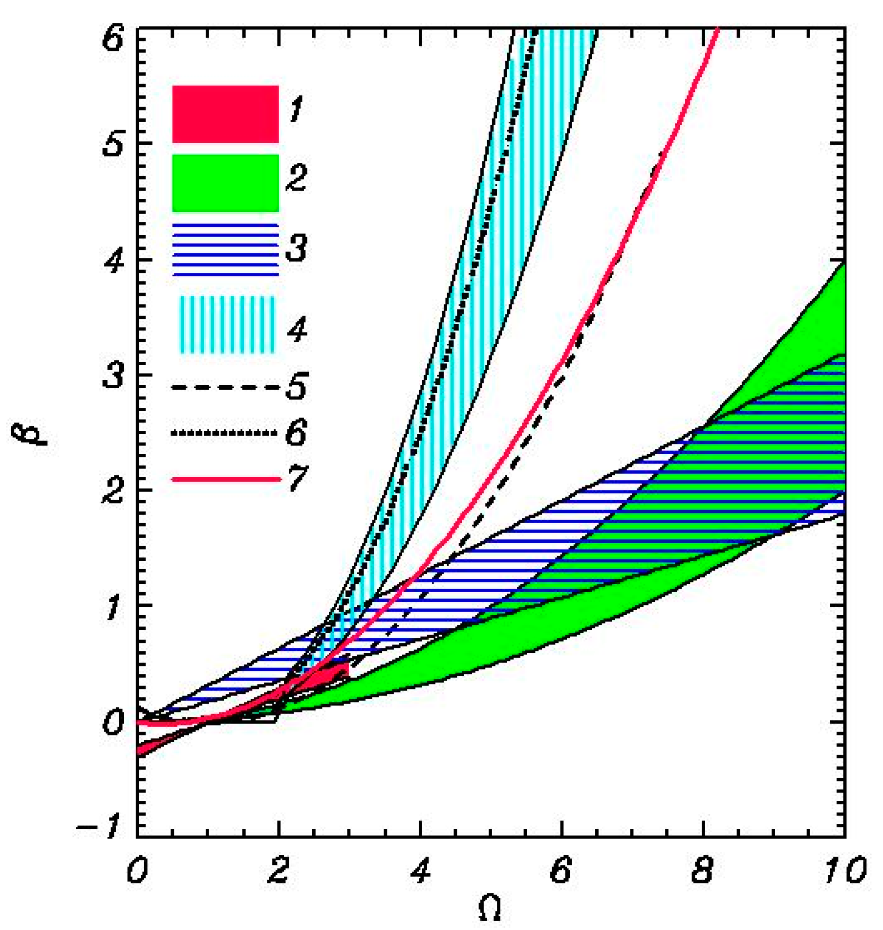
Different versions of the experimental -function are given in Figure 1. As seen, the values differ by several times. The function calculated in [17] which is discussed below is very close to a relatively old version [30]. Naturally, such an agreement does not confirm the trueness of both approximations. Figure 1 demonstrates that the problem of wind-wave interaction is very far from being resolved. However, it is not surprising that the wave prediction models using such different recommendations generally give satisfactory results. The evolution of waves occurs under the influence of two competing processes: input energy and its dissipation. Dissipation is even more complicated than the input energy. Therefore, the parameters regulating dissipation as well as the entire scheme can be modified in broad limits. Finally, the comparison of wave forecast with the available experimental data gives the possibility to compensate inaccuracies in both schemes for obtaining an acceptable result.
The second way of the -function evaluation is based on the results of the numerical investigations of the statistical structure of the boundary layer above waves with use of Reynolds equations and an appropriate closure scheme. In general, this method works so well that many problems in the technical fluid mechanics are often solved using numerical models, not experimentally [12,38]. This method was being developed beginning from [6,8], followed by [9,39,40,41]. The results were implemented in the WAVEWATCH model, i.e., a third-generation wave forecast model [13], and thoroughly validated against the experimental data in the course of developing WAVEWATCH-III [14]. This method was later improved on the basis of the more advanced coupled modeling of waves and boundary layer [17], while the beta-function used in WAVEWATCH-III was corrected and extended up to high frequencies.
In our earlier works (see review [8]) the surface was assigned as a superposition of linear modes with a prescribed spectrum. Actually, the shape of the real wave is influenced by nonlinearity: the wave crests are high and sharp, and the probability distribution of elevation deviates considerably from Raleigh distribution. Also, the waves demonstrate a tendency for nonlinear sharpening [42] and breaking. All these features strongly modify the wave drag. A more realistic description was used in a model [17] where the model of WBL was coupled with a nonlinear phase-resolving wave model. Both models were written in the surface -following conformal coordinates. The 2-D WBL model was based on Reynolds equations and the energy/dissipation closure scheme; the solutions were matched at the interface. The initial conditions for waves were assigned as a random superposition of Stokes waves which amplitudes corresponded to JONSWAP spectrum. The description of the models and the numerical scheme can be found in [18].
One of the aims of the above investigation was the evaluation of function in a wide range of nondimensional frequency . For such purposes, 47 long-term (up to several hundred peak wave periods) numerical runs with the different wind velocity and spectral resolution were performed using the coupled wind-wave model. Wind velocity was assigned through the different values of wind stress at the upper level directed along and against the general direction of waves. The non-dimensional peak wave number was in a range (−28, 16), while the non-dimension wave numbers were in a range (−50, 50). The total number of Fourier amplitudes for the surface pressure and surface elevation falling in this interval was equal to 1,390,100. For the estimation of values, the above interval was separated into 100 bins with width . The number of points falling within each interval was roughly the same, i.e., around 1400. Generation of such large ensemble was necessary because together with the wave-produced pressure fluctuations the signal included a wide range of the pressure fluctuation caused by nonlinearity.
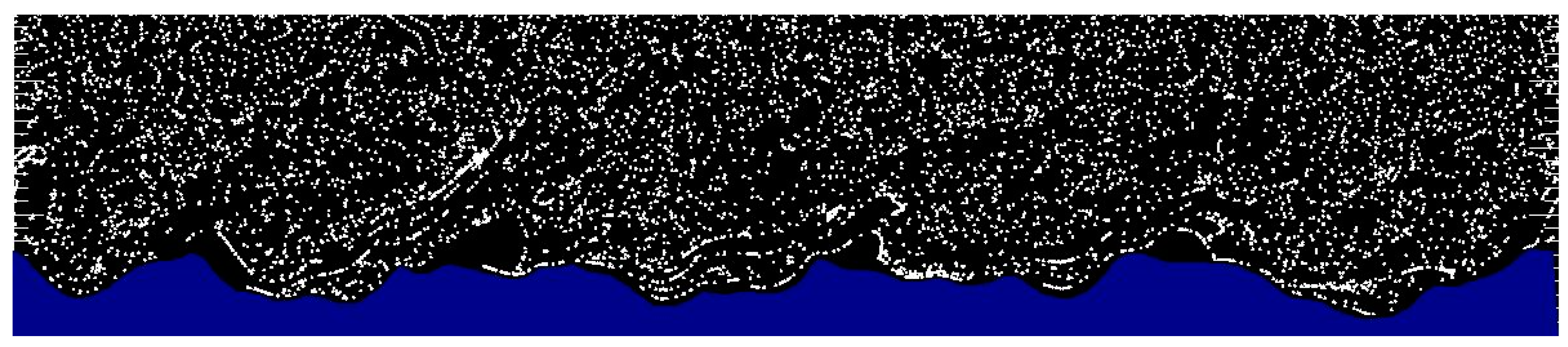
The structure of flow in WBL is illustrated by tracers that were initially placed in the cells of the regular conformal grid. The trajectories of tracers are not affected directly by turbulence, otherwise they would be less regular, and so, they are carried by the averaged flow. It is seen that separation of flow is a frequent phenomenon; it often happens behind more or less steep waves, but not necessarily after the breaking. We believe that the overflow of breaking waves is very similar to that of steep non-breaking waves. The events of breaking essentially modify the distribution of pressure and all these cases are, in fact, taken into account in the parameterization of the surface pressure distribution described below. Not that a picture in Figure 2 is remarkably similar to the pictures with tracers obtained in a laboratory wind-wave channel (described in [43]).
We found that the processing of the signal done in a paper [17] was not accurate enough and was repeated here with some improvements. Note that the data described above were obtained with an undirected model. It is why in the equations below, the index is omitted. Before calculating of values we performed filtration of the data excluding the points with an excessive deviation of a mean value. In one-dimensional wave field the one-point values of real and imaginary parts of -function can be calculated through the Fourier coefficients for and for each bin :
while the averaged values of and were calculated in each bin with i number using rms method:
where is the number of points falling in each bin.
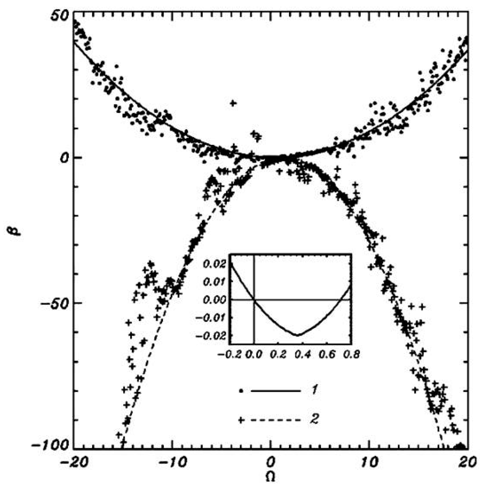
The data marked by dots and by the + sign show the imaginary and real part of function . A fragment in the middle of Figure 3 shows an imaginary part of function .
The data obtained in [17] fall in the interval . However, the scatter of the data outside this interval is large, hence, the approximation of -function may not be accurate (though, in our opinion, it is still acceptable). Usually, such high values seldom occur. The imaginary part of function is negative in the interval where the phase velocity of waves is larger than the wind velocity; hence, the momentum and energy are transferred from waves to wind. It means that the pressure at the upwind slope of waves is less than the pressure at the downwind slope; hence, waves accelerate wind and lose their momentum and energy in a vicinity of .
In all other intervals of the flux of energy and momentum is directed from wind to waves, i.e., the pressure at the upwind slope of a wave is larger than at the downwind slope what decreases the absolute value of wind velocity. The flux of momentum is directed to waves, but the wave momentum is negative, hence, the waves decelerate, and the energy dissipates. In the cases when wind blows against waves, the function is larger than in the opposite case with the same value of , so the function is not symmetric regarding . The processing of the large volume of data generated in [17] based on Equations (9)–(11) gave the approximation:
where , , , , , .
The -function can be represented as a dependence of time scale for energy input for the modes with nondimensional wave number , normalized by period of mode :
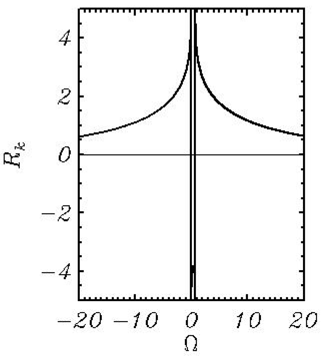
(here the imaginary part of is included; and are densities of air and water). The Equation (14) gives an estimation of the timescale for the rate of wave growth in terms of wave period as a function of . This function varies by orders and has both positive and negative values. Therefore, it is convenient to use the following transformation:
For estimations, formula can be used. Vertical lines at and correspond to the zero values of (see inset in Figure 3) and infinite time scale. Timescale is everywhere positive, which means that energy goes to waves. It is negative (an inverse flux of energy) in a narrow interval where waves give their energy to air at the timescale of the order of .
The same order of value has a positive timescale for small frequencies. For the timescale for input is of the order of 10, while for the timescale is as small as few periods of mode. It means that only low-frequency waves, typically in the peak of the spectrum, are conservative, but high-frequency modes in the tail of the wave spectrum are short-living. Because the shape of the tail is more or less steady, the rate of dissipation in the spectral tail is also high. Consequently, the suggestion that the spectral tail is mostly formed of the nonlinear cascade of energy cannot be confirmed. Note that the approximation suggested in [33], (Figure 1) gives unrealistic small-time scales, i.e., by orders smaller than in Figure 4.
The non-stationarity of wave modes as well as the non-linearity of wave field as a whole (e.g., the tendency for being a superposition of Stokes-like modes), variability of phase velocities (see [44]) and the presence of the broad spectrum of pressure fluctuations of non-wave nature all indicate that the connection between and is not deterministic. This is why the calculations, (10), (11) based on the results of many runs with different initial conditions and wind velocities give an effective shape of -function, which, in fact, implicitly takes into account most of the complicating factors mentioned above, including the effects of random flow separation. The time scales of these processes are much smaller than those for energy growth [44]. This is why we tend to treat Equation (4) not as a connection between instantaneous amplitudes of pressure and elevation but rather as a connection between the quantities averaged over time and over some frequency intervals.
4. Wave-Produced Momentum Flux
The existence of interface dictates to use the surface-following coordinate system where the vertical coordinate at . Above the flat surface the natural boundary condition is a zero vertical velocity, i.e., . In the conformal coordinates the role of vertical velocity is played by the contravariant component of velocity ([15,18]). The kinematic condition on surface suggests the absence of exchange through the surface by finite volumes.
An equation of evolution of horizontal momentum can be obtained by averaging of equation for component of velocity along the coordinate lines . Brackets denote the averaging (see details in [18])
Since , and , Equation (16) can be considered as written in the Cartesian coordinate system.
According to (16) the rate of evolution of horizontal momentum depends on vertical divergence of vertical momentum flux generated by wave-produced components of velocity , by pressure and by the averaged turbulent flux .
Equation (16) is analogous to the equation of momentum balance above flat surface
which, in fact, is used in linear theories and can be obtained by averaging in the Cartesian coordinate system above sea crests. Equation (17) is useless since it does not include wave effects. Note that the averaging in a surface-following coordinate system is physically performable both in the laboratory [32] and the field [33].
Let us represent Equation (16) in the form
where is a wind profile, is a turbulent momentum flux, and is the Wave Produced Momentum Flux (WPMF). Vectors and are directed along x axis.
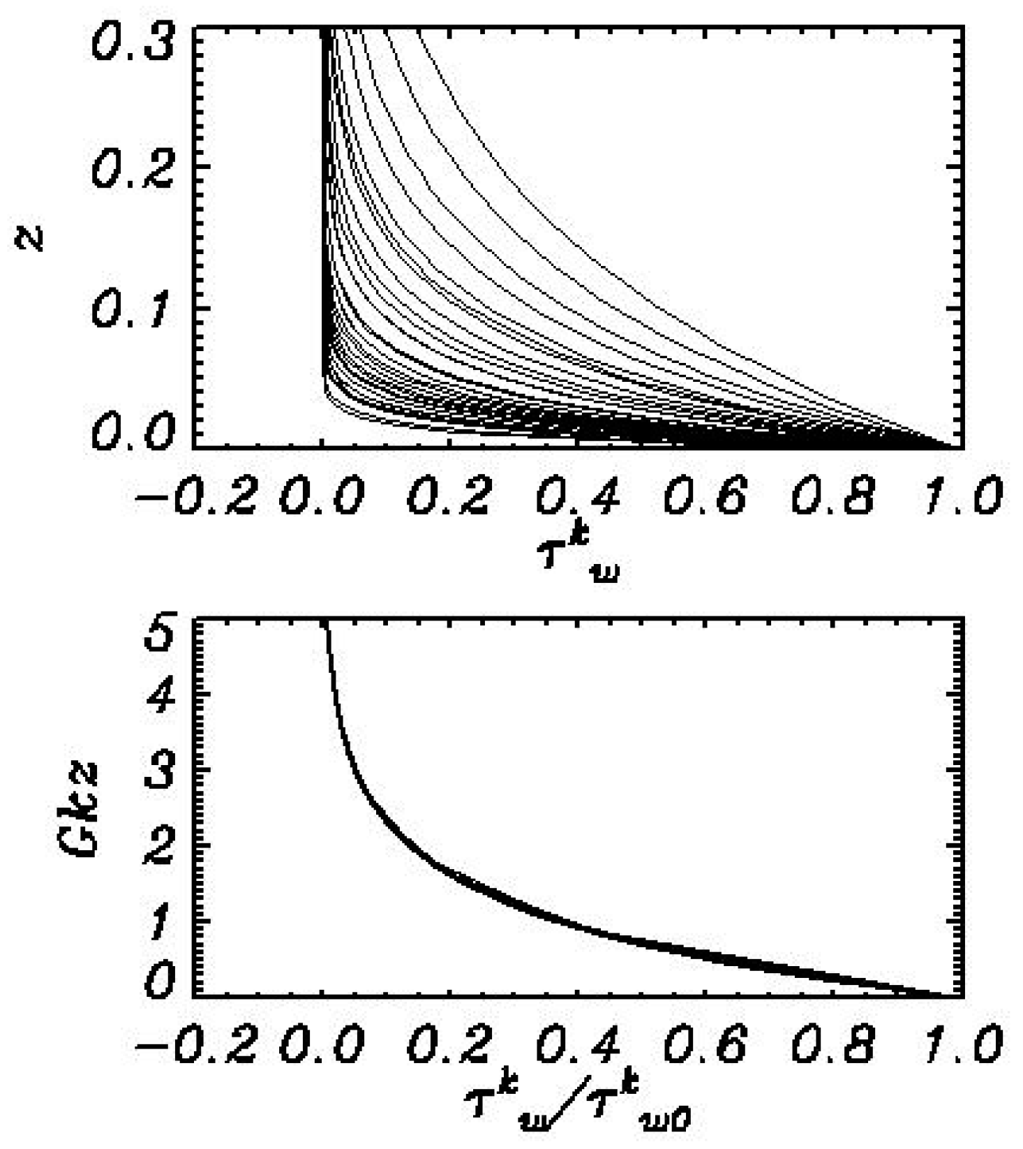
The vertical profiles of WPMF were investigated in detail in [17], where the numerical experiments with the coupled wind/wave model were described. A wave boundary layer (WBL) model is based on Reynolds equations with the closure scheme. The solutions for air and water matched through the interface. The structure of the WBL and vertical profiles of the wave-produced momentum flux (WPMF) in a long-term simulation of the coupled dynamics are investigated and parameterized. The averaged profiles of spectral components of WPMF calculated in [17] are shown in the top panel of Figure 5 reproduced from [17]. As seen, the shape of those profiles depends on the wavenumber. These data can be arranged by normalizing each profile by its surface value and representing them as a function of nondimensional height. After that transformation the profiles converge. The convergence can be even closer when by introducing the following relation:
where G is a function of
Note that at the moderate spectral resolution the introduction of function G in (19) changes the result insignificantly, hence, in such cases it is possible to put . The profiles of spectral components of are given in the bottom panel of Figure 5 as a function of (20). As seen, Formula (19) demonstrates a good approximation of vertical profiles of WPMF.
5. One-Dimensional Model of the Boundary Layer above Waves
The WBL is defined as the lowest part of the atmospheric boundary layer where a considerable part of momentum and energy is transferred by fluctuations of velocity and pressure produced by waves. The WBL height is of the order of several significant wave heights, typically of the order of 10 m. In the bottom, WBL adjoins the wave surface and in top it merges with the stratified Monin-Obukhov boundary layer. In the majority of cases the WBL height does not exceed the height of the dynamic sub-layer, so it is not necessary to take into account the effects of stratification, though these effects can be easily included in the model below. The equations of non-dimensional WBL were derived in [17] with an averaging of two-dimensional equations in the conformal coordinates along the coordinate lines. Here we present a more general case considering velocity as a vector velocity with components :
where is a vector of vertical WPMF; e is kinetic energy of turbulence; is the coefficient of turbulent viscosity ( is Karman constant); τw—wave-produced momentum flux; P—a rate of turbulent energy generation:
In a previous version of the model the system of equations included an equation of evolution of the dissipation rate together with the formula written with dimension consideration. Fortunately enough for the current problem this equation is not required as it does not change the results noticeably. In fact, this equation does not seem to be physical, and in complicated problems it often gives unrealistic values removed with the use of the so-called ‘limiters’.
In the current work the averaged over horizontal domain structure of the wave boundary layer above wave surface assigned by a two-dimensional wave spectrum () is under consideration. Axis is directed to East, while axis —to North. The frequency varies in the interval , the wave direction changes counterclockwise in a range . The frequency grid is set with the three parameters: number of intervals , top value of frequency and stretching coefficient
At the upper bound of domain the components of wind velocity are assigned:
where is wind velocity; is direction. In the description of wind-wave interaction in Section 2 it was accepted that direction of wind coincides with k-axis. It is assumed that WPMF attenuates at and the value of turbulent energy at is proportional to the turbulent stress
where and are the components of horizontal stress; is a constant. The same rule is used for calculation of the energy of turbulence at the lowest level :
The equations of the WBL model are approximated at the irregular stretched grid where is a stretching coefficient. In a research version of the model considered here, the height of the domain was 10 m, the number of levels in the air was equal to 50 and the stretching coefficient was taken as . The variables and placed to the middle of the layers; their fluxes and wave-produced momentum flux were placed in accordance to the intermediate levels. A high value of was used for setting a high resolution close to the surface so that the thickness of the lowest level was of the order of height of the viscous sub-layer ( is a molecular air viscosity and is the local friction velocity). In this case an effective roughness parameter can be calculated with Formula [11].
The local surface drag coefficient , surface tangent stress and local friction are calculated by a formula:
The method of WPMF profile calculation requires more detailed consideration.
Typically, the wave spectrum contains thousands of values of wave energy. For calculation of the energy input to each interval it is necessary to calculate the wind velocity value at level . Since the vertical grid is irregular, this simple operation procedure turns into a big problem, especially, if the WBL model is used for the coupling of the atmosphere with the wave model or ocean model. A simple way to overcome this problem is the approximation of wind profile , for example by a relation:
where
where coefficient is calculated by the root mean square method:
where the summation is performed over the vertical coordinate. Formula (29) with coefficient A is used for calculation of the interpolated and extrapolated values of wind velocity :
at height:
where , and is an angle between the wind direction and the direction of kth mode. The function is included in a reference level because waves moving at angle to the wind direction have a corresponding longer virtual length. Note that Equation (32) can give unnaturally high values of , especially for the low-frequency waves. We restricted this quantity by limit which did not influence the results.
The nondimensional frequency is calculated by a formula:
These values of are used for the calculation of an imaginary part of -function (12). The components of surface momentum fluxes from air to waves are calculated with the formulae:
The flux of energy to waves in the spectral cell is calculated by formula:
Here, in Equations (35)–(37) is the imaginary part of -function of (34) calculated by (12). The 1-D spectra of the surface wave flux of momentum and can be calculated by summation over angle
while the components of total wave flux—by summation over frequencies:
The total flux of energy to waves is calculated by summation over angles and frequencies
The vertical profiles of WPMF components are calculated taking into account the exponential attenuation (19), (20):
where is the virtual wavenumber (i.e., taking into account the direction ):
and is the function (19).
Note that in the above equations, a variable with two indexes denotes matrix; with one index it denotes the same variable but vector obtained by summation over angle; and with no indexes–the variable denotes scalar obtained by summation over angles and frequencies.
6. Examples of the Calculations for Idealized Spectrum
A model formulated above is designed for the calculation of the drag coefficient that can be used for estimation of fluxes specific feature of the model is that it links the structure of WBL with the upper boundary condition and any arbitrary wave spectrum.
Below are the results of the calculations performed for the cases when surface waves are assigned by JONSWAP spectrum [45] for different wind velocities and inverse wave age ( is a wind velocity at height , is a phase velocity in spectral peak).
Here is a one-dimensional spectrum and is a function describing the angle distribution of the potential energy density.
where ( is frequency in spectral peak), is a coefficient depending on [46]
and is a function of :
The angle spreading is taken in a form suggested by Donelan (1999).
The shape of spectrum depends on and on the frequency in spectral peak
A wave spectrum was assigned at grid at stretched grid with a stretching coefficient ; in the interval with a constant step over angle . The WBL model was approximated at grid with a number of levels at with a stretching coefficient . Such a high number of level and value provided a high resolution close to the surface which justified a use of the roughness parameter for smooth surface (27).
A steady numerical solution of Equations (21) and (22) was obtained with a second order scheme over and an explicit time integration scheme. Such a scheme requires a very small time step estimated by condition:
For steady conditions the total flux of momentum should be constant over height
Note that a term in Equation (50) at should be replaced by the term (see Equation (28)). The criterion of steadiness was chosen is a form:
where is the total flux of momentum at . An explicit scheme was used here because the solution was very fast. However, when the model is used for massive calculations together with another model (for example, with a wave forecast model), it is reasonable to use the TDMA method [47].
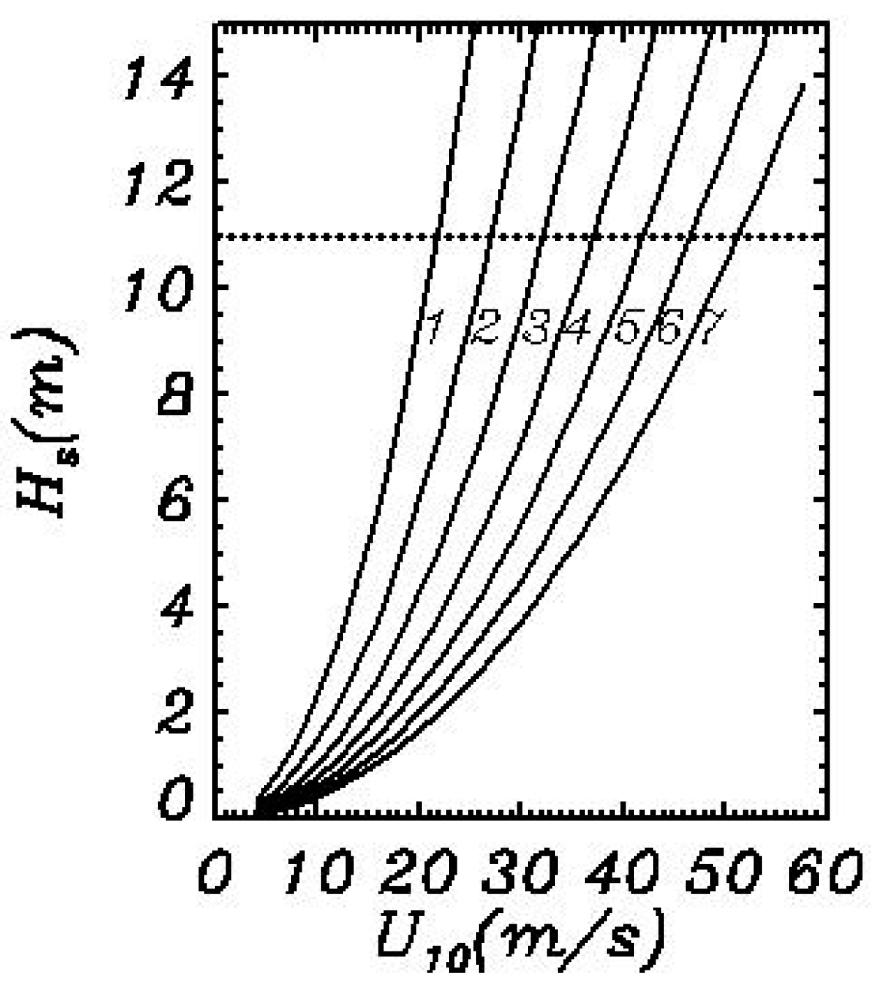
The structure of WBL is illustrated in the cases shown in Figure 6. The area of unrealistic value of the significant wave height corresponding to the wave height about 33 m is separated by a dotted line. This area will be shown for other characteristics of WBL.
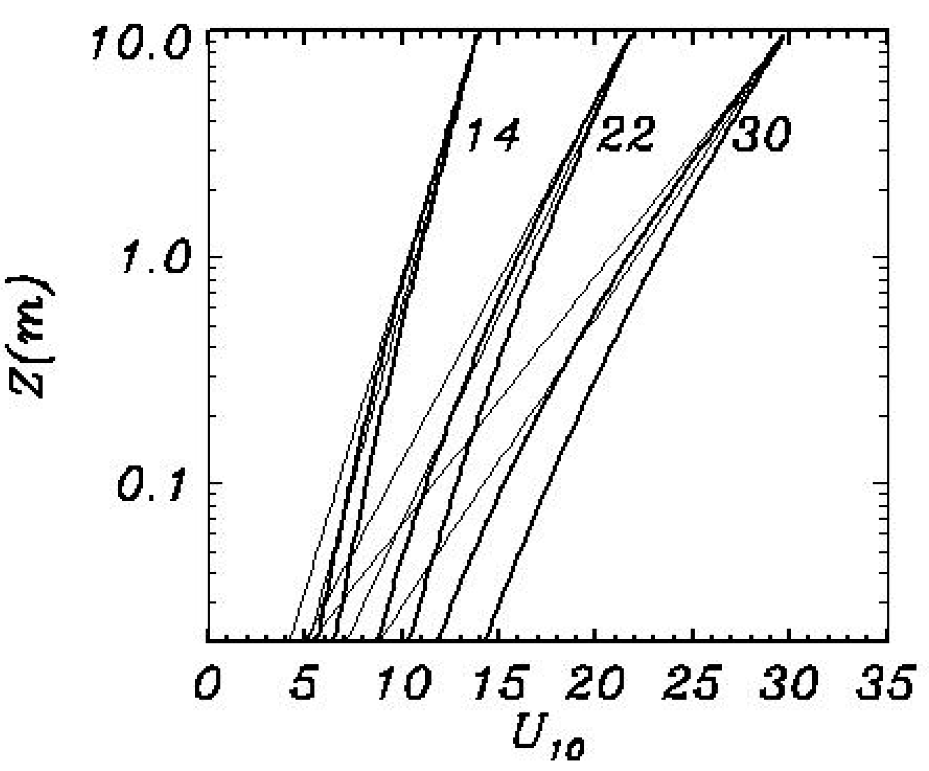
The wind profiles shown in Figure 7 demonstrate a considerable deviation of the logarithmic behavior (described by the second term in Equation (29)). For a smaller wave age (larger ) the deviation is larger and can be as big as for .
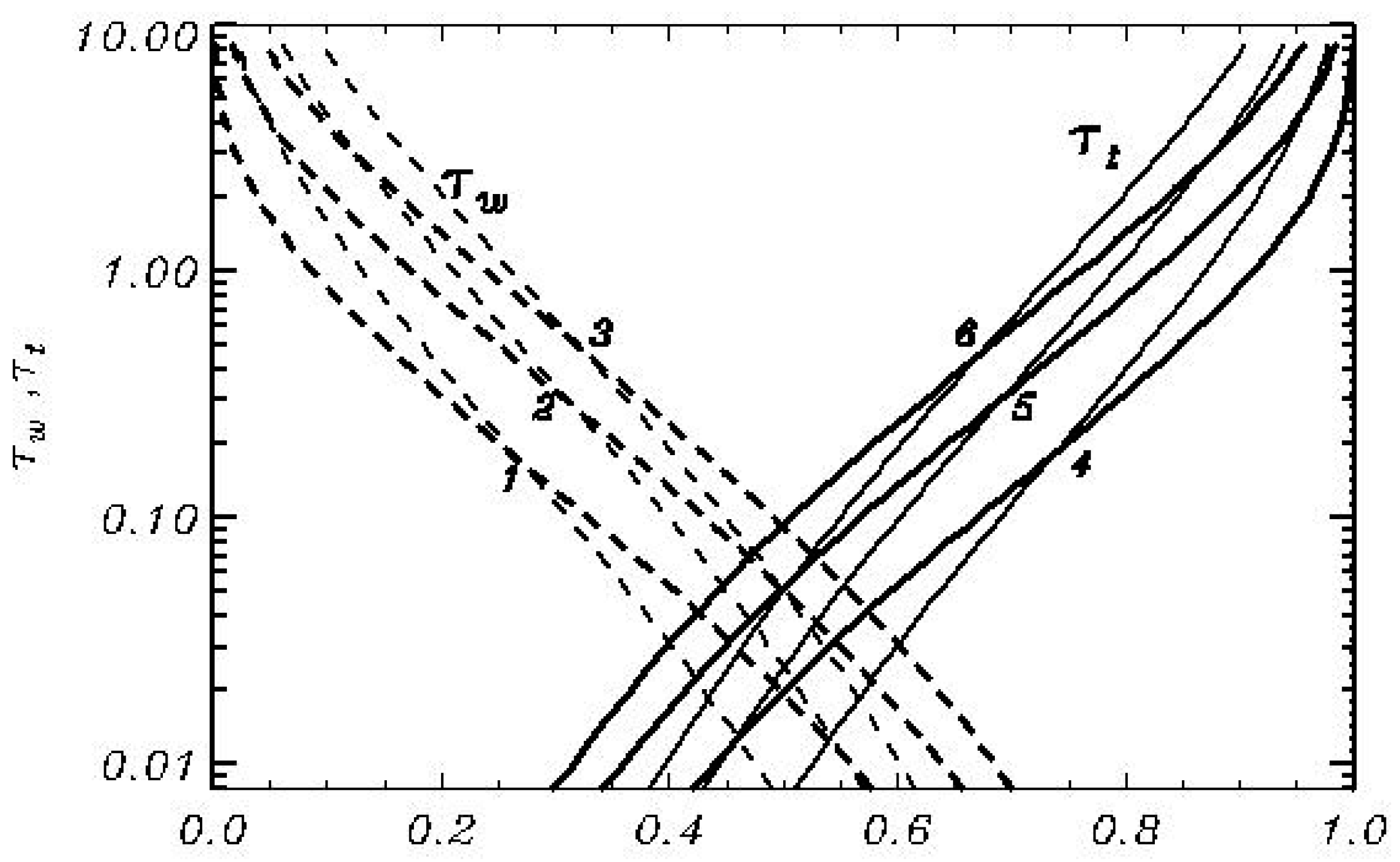
The specific property of WBL is that the mechanism of momentum transfer to wave develops very close to the surface. Figure 7 shows that deviations of the logarithmic wave profile are concentrated below the height of 1 m. It proves that the main part of momentum is transferred by small waves at high frequencies. The main advantage of a one-dimensional approach is that it allows a broad range of frequencies to be taken into account and most part of the wave produced flux. Contrary to the turbulent stress, the wave produced flux of momentum is generated directly by an external factor, i.e., by curvilinearity of a moving surface. In a steady boundary layer the vertical flux of momentum should be constant over height; hence, the turbulent momentum flux should decrease when approaching the surface, and the connection between the stress and wind profile is modified (Figure 8).
As can be seen, a decrease of turbulent momentum flux is completely compensated by the increase of WPMF that when close to the surface, can reach values as high as 0.7. For the wind that is less than 20 m/s, the WPMF turns into 0 at the upper level. For higher winds, the WPMF can reach a value of , which means that the total height of WBL is higher than . The calculations with the increased height of domain up showed that the results in the layer obtained at complete attenuation of WPMF to the upper level are very close to the current results. Since is a standard reference level, we keep to this value for all variants of calculations.
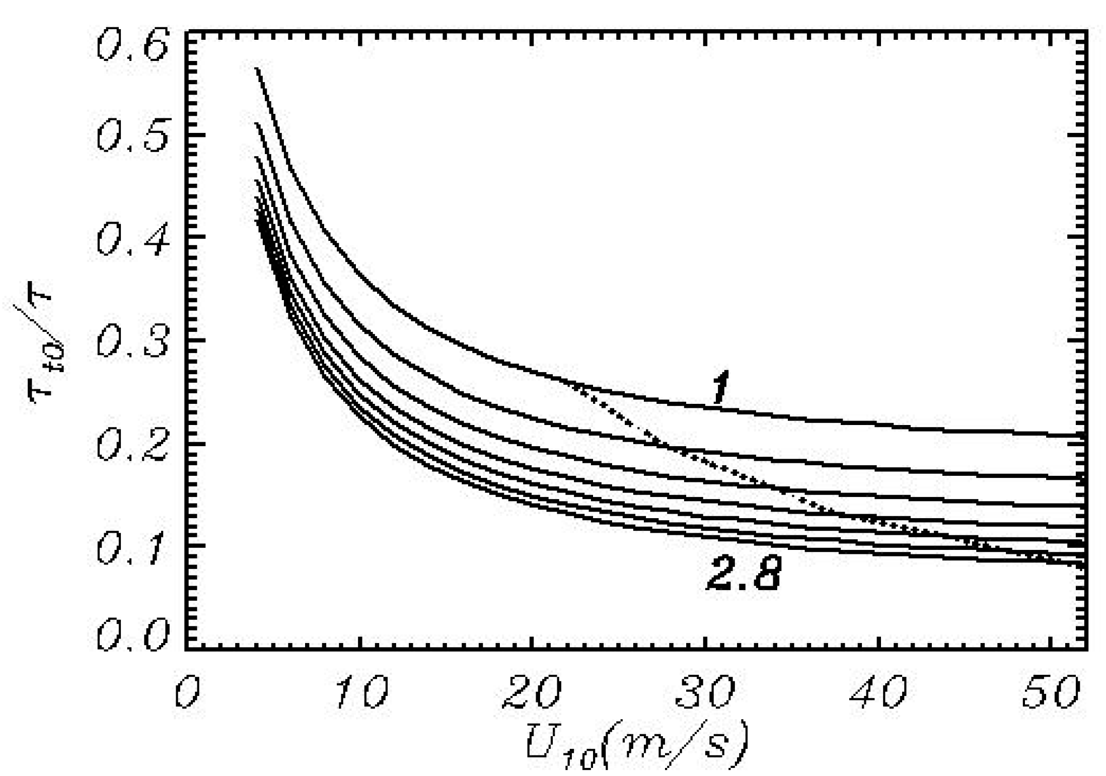
The role of surface tangent stress calculated with Equation (28) is illustrated in Figure 9. The contribution of tangent stress in the total surface stress is large for small wind and increases with growth of inverse wave .
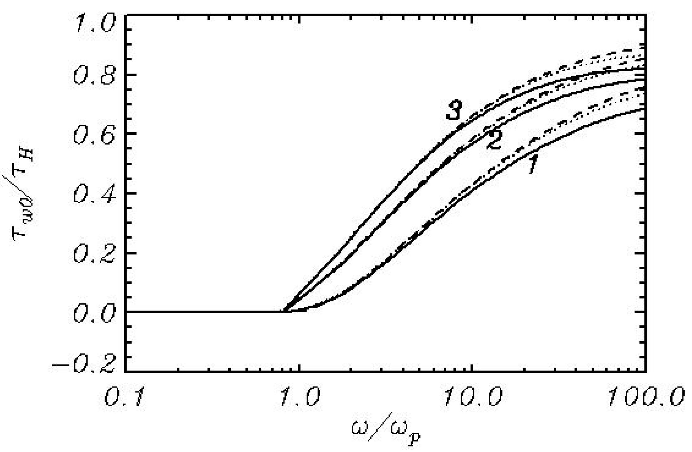
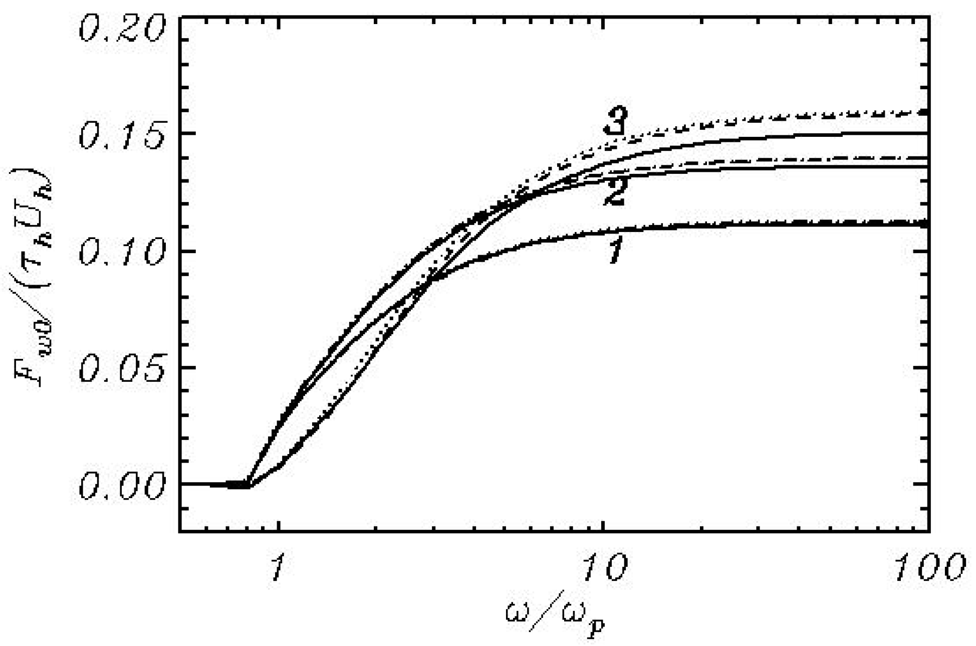
The dependence of these quantities on nondimensional frequency is shown in Figure 10 and Figure 11. As seen, both pictures demonstrate a great contribution of high-frequency modes to the fluxes. The spectral composition of the surface momentum and energy fluxes is convenient to consider their integrated values and as a function of the upper limit :
where is the total vertical flux of energy at .
The flux of energy comes to the saturation level at while the flux of momentum remains growing up to . It can be explained just by dimensional consideration: Equations (35) and (36) contain , while an expression (37) contains . The tendency for the tangent stress to drop at high frequencies in Figure 9 and the tendency of fluxes to increase in Figure 10 and Figure 11 can be explained by an insufficient resolution. This effect could be reduced by introducing a higher resolution in frequency, but a shape of the -function for high frequencies is not well known. However, the total stress as a sum of and is calculated correctly.
The stationary solution for WBL can be obtained without separation of subgrid stress into a tangent and WPMF part by assuming that a total stress on surface is equal to the outer stress .
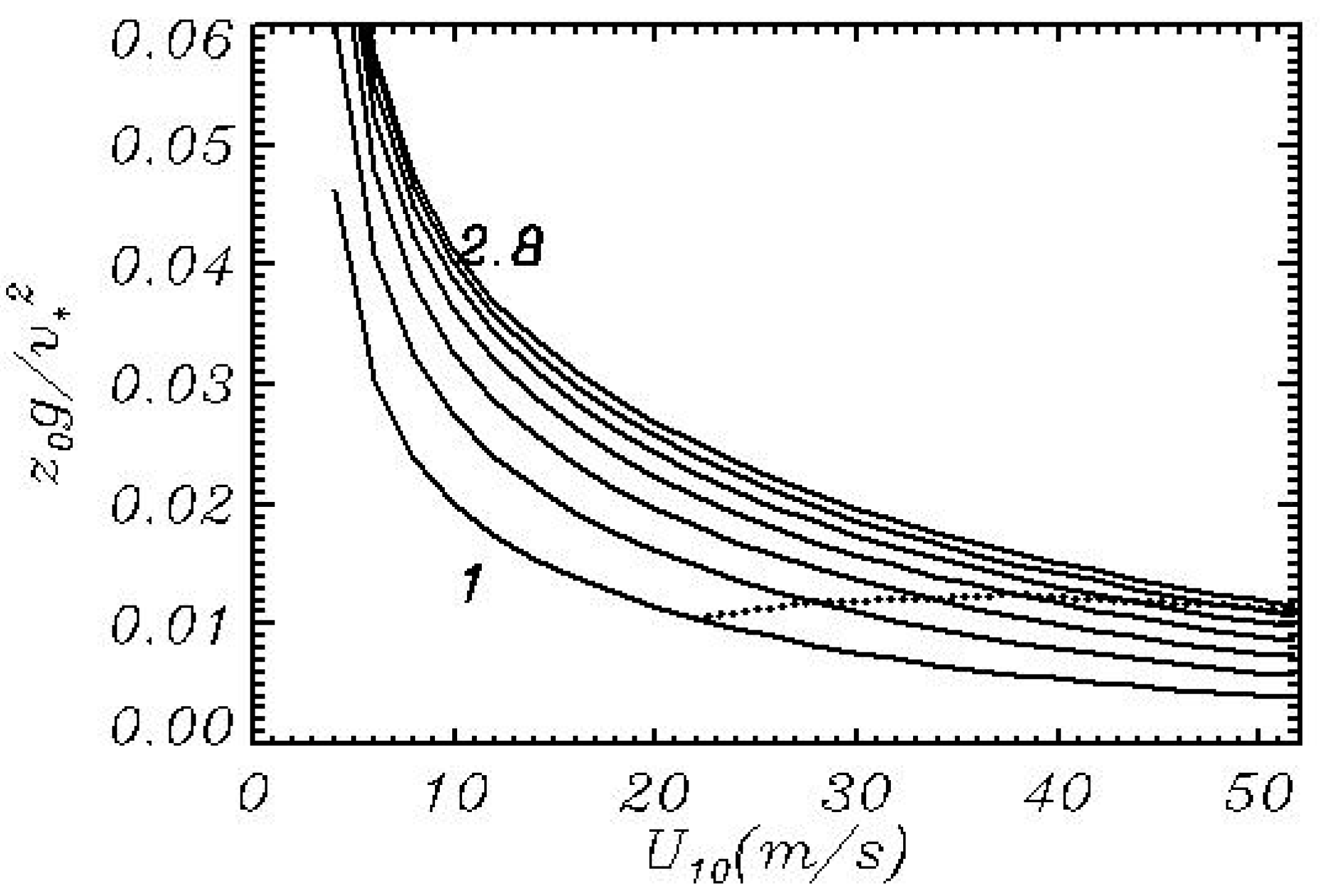
Such formulation of the WBL problem does not require the use of high resolution in and . However, this scheme cannot be recommended for the precise calculation of wind-wave interaction, since WBL is not always fully adjusted to waves, and the sum of turbulent momentum flux and WPMF is not constant over height (see Section 5). In general cases, the WBL can be unsteady. The nondimensional roughness parameter is calculated by relation
here is plotted in Figure 12. As seen, is not a constant but significantly depends on wind velocity and inverse wave age .
The JONSWAP wave spectrum depends on the two parameters, i.e., wind velocity and inverse wave age . Hence, the drag coefficient also depends on these parameters: the dependence on is direct, while on inverse wave age it depends because the larger , the larger the steepness of the wave field which can be defined as follows:
where is a wavenumber. Naturally, is nondimensional, but for its value depends logarithmically on cut-frequency . This is why cannot serve as an absolute characteristic of wave field, but it is useful for the comparison of the wave fields with the same spectral resolution. In our case for it equals 0.25 and for it is 0.3. This difference is large enough to consider that the dependence on might be significant. The dependence of on turns out to be quadratic (Figure 13). For the developed sea () it does not exceed , while for the young sea it reaches the value . A comparison of these results with the experimental data is easy, as the existing data due to a large scatter can confirm any reasonable results.
The dependence of drag coefficient on wind was studied in laboratory ([48,49]) and field ([50,51,52,53]). In general, these data show that at least up to the drag coefficient grows (see the data collected in [54]). The values at wind velocity fall in the interval . Above the value the drag coefficient in compliance with the majority of recent data starts to drop. According to [54,55] the drag coefficient can be influenced by swell. Different functions were tested being implemented in coupled models [56,57,58,59,60,61]. Those studies showed that introduction of a drag coefficient decreased at strong wind improves the forecast results.
The data from different sources being plotted together (see [54]) look chaotic. The data can equally prove and disprove any reasonable theoretical scheme. A reason for this is an absence of ideal conditions when the theory is applicable. There are many reasons why the vertical flux of momentum is not a constant over height. For example, in a specially selected area for conducting a study of the Monin-Obukhov boundary layer the conditions during the vertical flux of momentum changing twice over the distance of 10 m, was not unusual. The cause of such a phenomenon was a forest at a distance of 2 km from the point of observations, which violated the condition of horizontal homogeneity (A.M. Obukhov, private communication). Finally, it looked as if the drag coefficient depended on wind direction. Sea conditions are usually closer to homogeneity, but the deviation can be created by meso-scale wind and sea surface temperature disturbances as well as by secondary circulations in the planetary boundary layer and upper ocean, and for many other reasons. If the wind profile is not logarithmic, the value of drag coefficient can change unpredictably in a broad range.
If the sea surface is flat at the conditions of stationarity and homogeneity, the structure of the boundary layer is very simple and can be described by the well-known formulae. Hence, even at ideal conditions in the presence of waves the drag coefficient is a product of waves. Wave spectrum is seldom described by the JONSWAP approximation [45]; it often contains more than one peak. Also, a general direction of waves can deviate from the wind direction. The angle distribution even for the JONSWAP approximation is not well known. The drag coefficient depends on many factors:
1. A specific shape of the spectrum. The spectrum can have more than one maximum; it contains swell and high-frequency tail. The spectrum can be asymmetric about wind direction, and the general direction of energy-containing waves can deviate from the wind direction. The data on time scales for the energy input (Figure 4) show that high-frequency waves should be adjusted to the local wind conditions and are most likely generated by the local in time and space wind.
2. The local non-stationarity and non-homogeneity are caused by change of wave spectra and wind velocity. In this case wind profile is not adjusted to the local wave spectra and can considerably deviate from the structure shown in Figure 7. At the time scales of a governing model the WBL can be also nonstationary, hence, we cannot rely on stationary solution.
Great variations of drag coefficient can be observed in the complicated processes such as tropical storms where waves are not directly connected with local wind, and the conditions are very far from being homogeneous and stationary. In this case, the characteristics of ocean-atmosphere interaction are the product of local wind and waves as well as of the prehistory of the process. Definitely, drag coefficient should be different in the different phases of storm. It means that this process should be described not by the selected formulae and rules, but by a system of the equations describing a dynamic interaction between the atmospheric boundary layer and upper ocean taking into account sea waves.
7. Pragmatic Model of the WBL
A one-dimensional WBL model described above is not convenient for regular use in a frame of the ocean-atmosphere-sea wave models because it is based on direct calculations of high-frequency waves and tangent stress in a viscous sub-layer. Hence, the formulation of such a model suggests a high resolution for wave spectrum and for vertical coordinate. Such a model is well suited for research. The spectral wave models usually do not include high-frequency waves. Besides, the high resolution WBL model being included in a large model takes considerable time, which can slow down the entire process. The straight way to avoid such a problem is to assume the stationarity of WBL. In this case WPMF for the wave modes included in wave spectrum are calculated directly with Equations (41) and (42), while a surface boundary condition for turbulent stress is taken in a form:
following from the assumption of the homogeneity and stationarity of the WBL. With such formulation the WBL model can use a poor resolution by vertical (about 10–20 levels). This approach is too simple to be universal, because the real process is seldom close to the conditions assumed, hence Equation (56) is, in general, inapplicable. However, the ocean-atmosphere and wave modeling require the formulation of a simplified approach, what we call here a ‘pragmatic’ model.
Let us consider a model of the WBL (21)–(23) for the calculation of the WBL structure above waves assigned by an arbitrary wave spectrum . The upper boundary conditions (24) and (25) remain unchanged. The principal difference between the research model and pragmatic model is that wave spectrum is assigned up to the relatively low frequencies, of the order of 1 Hz, i.e., the smallest wave has the length of the order of . We should admit that such spectral resolution is too poor for a good description of the WBL structure, because even the smallest wave with the frequency of 1Hz, is supplied by energy from a layer with the thickness of the order of WBL height. In fact, wave prediction models are the models of big waves. However, we hope that the resolution of wave models will be gradually improving, at least for research purposes.
Let us suppose that the wave model uses a grid with the maximum frequency . It means that the influence of waves with smaller frequencies is described individually in terms of the spectral components of momentum flux calculated with a use of -function. The influence of the subgrid modes with should be taken into account parametrically. Let us suggest that above frequency waves are generated by current wind; the spectrum is with respect to wind direction and the energy is falling down to . Such assumptions are not voluntary, since according to Figure 4, high-frequency waves have a small timescale, i.e., it would be reasonable to suggest that they are generated by local wind. Such situation can happen, for example, in a tropical storm when the wind quickly changes direction and starts to generate new waves. The problem is describing the total momentum flux to waves in the interval :
where
is an index of frequency and is a number of frequencies in the research model. The data on and were generated in a series of calculations with a high-resolution model for the JONSWAP spectrum. The parameterization means that the values of and should be represented in terms of the individually calculated variables of pragmatic model. There are several ways of obtaining such an approximation, and we chose a version that gives the smallest errors. We found that the stress produced by subgrid waves can be approximated by relation:
where ( is peak frequency), is the external friction velocity, while and are the functions of :
The tangent stress is approximated by relation:
where and
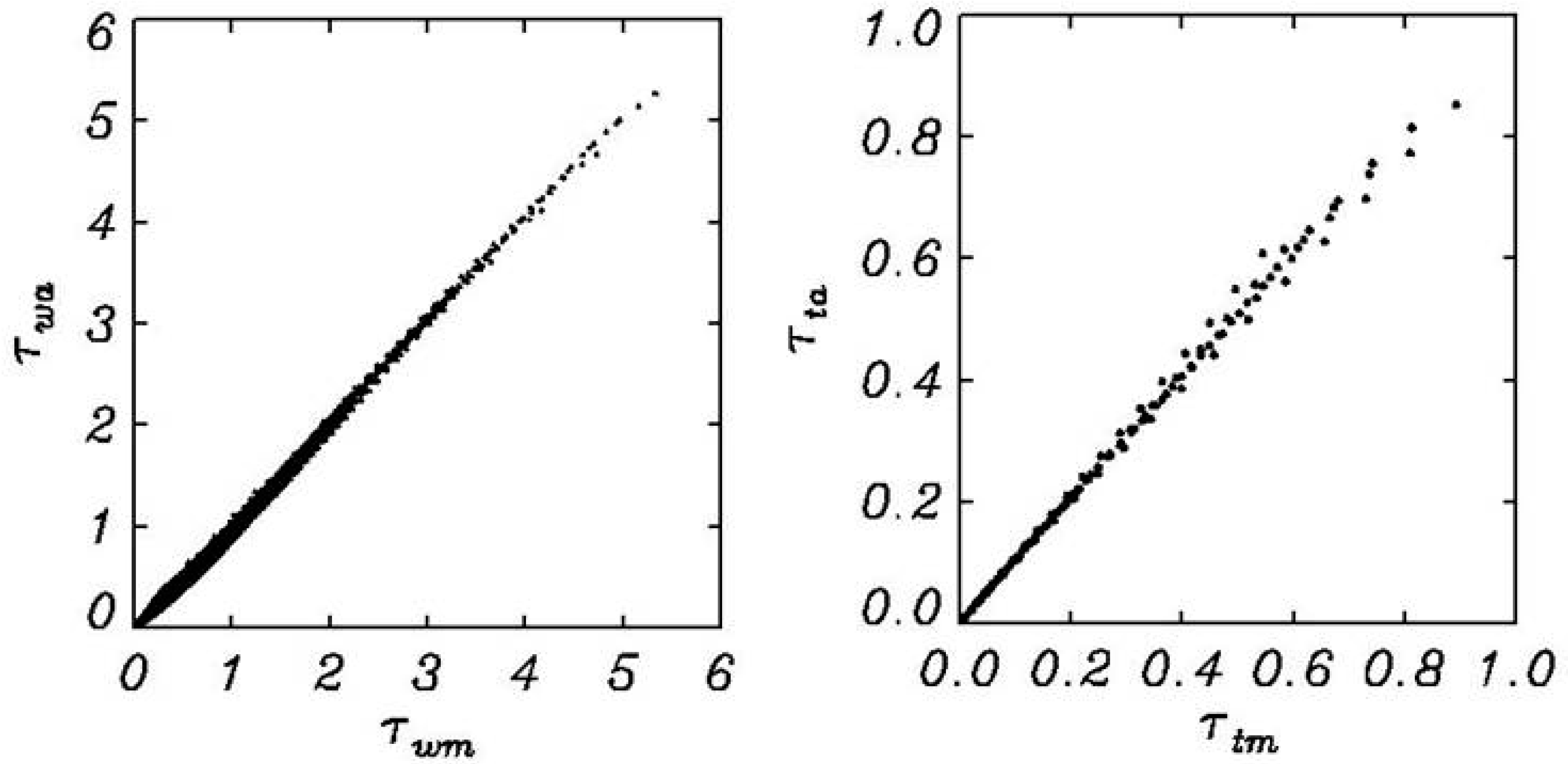
The approximations (59)–(62) are valid in a range and for the wind velocity . The accuracy of the approximations (59)–(62) is demonstrated in Figure 14 where the values calculated with (55)–(58) are compared with the model calculated with high resolution. It should be underlined that parameterization (59)–(62) is based on the assumption that parameterized high-frequency stress is produced by local wind.
8. Dependence of Drag Coefficient on Wind Direction
The model described above was used for illustration of dependence of drag coefficient on wind direction. It seldom occurs that wave spectrum is symmetrical and is produced by constant wind. In reality, wind often rotates and starts to generate its own wave system and provide by energy the existing waves. In a most clear form it happens in tropical storms where waves are a product of a rapidly changing wind system.
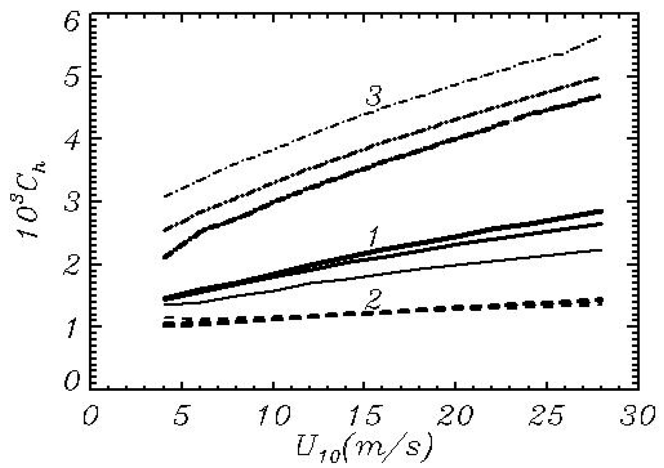
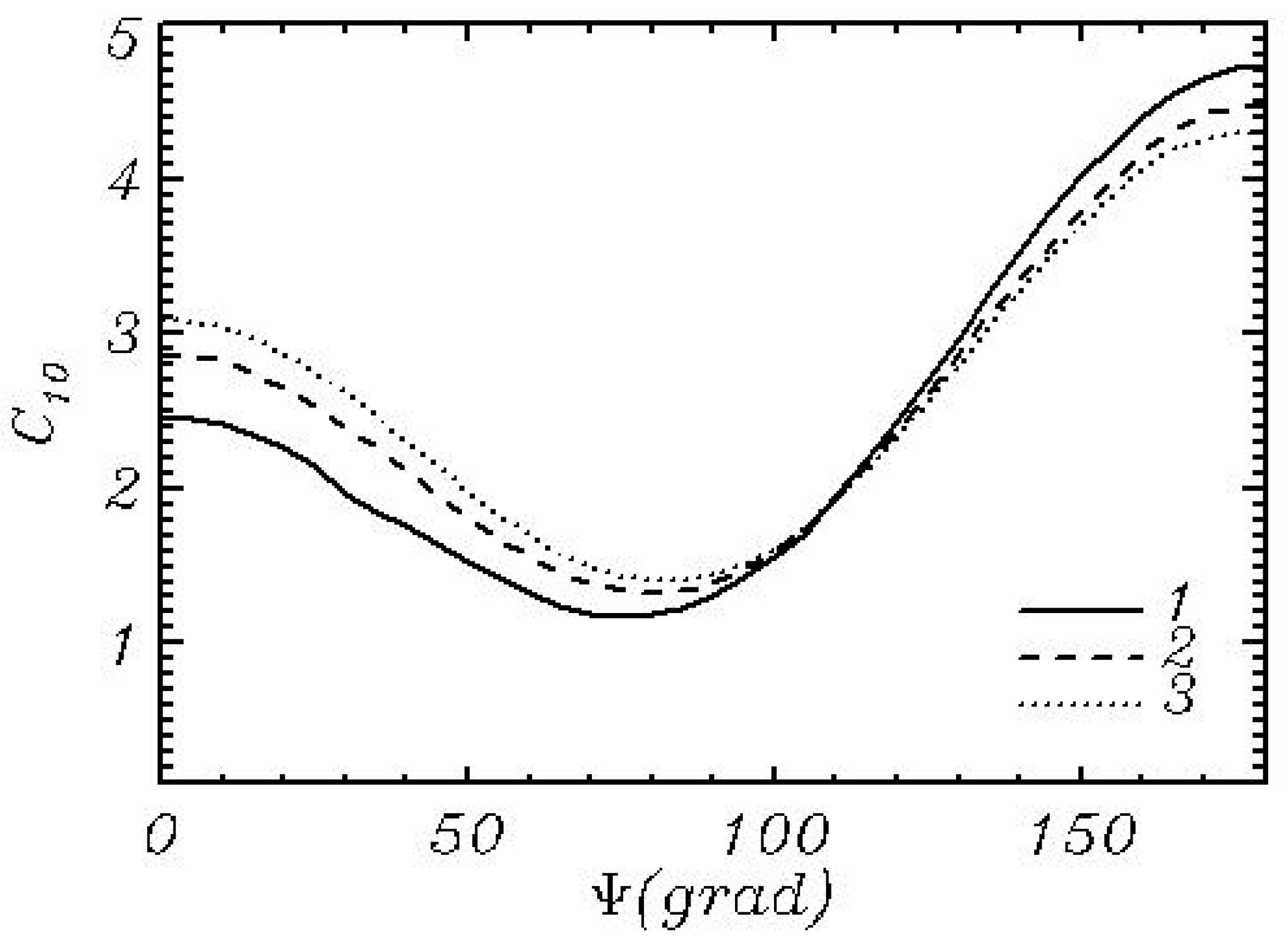
For the calculations a simplified model with modest resolution was used: the number of frequencies ; maximum frequency is ; the stretching coefficient ; the angle resolution . The WBL model was approximated at a grid with levels; the time step was estimated with Equation (48). The surface boundary conditions for the subgrid wave-produced momentum flux and were calculated by Equations (58)–(62). The wave spectrum in a range was assigned by the JONSWAP approximation. It was assumed that at higher frequencies the wave spectrum is also described by the JONSWAP asymptotic, but a general direction of such high-frequency waves coincides with the wind direction. The calculations were made for three values of inverse wave age: and ; for three directions of wind: (the directions of wind and waves are the same, curves 1 in Figure 15); (vector of wind is perpendicular to waves which are treated as a multi-mode swell); merging curves 2; (wind is directed against swell, curves 3). Curves from Group 1 are close to the same curves in Figure 13. Case 3 corresponds to the waves moving mostly perpendicular to wind. In this case the drag coefficient is supported by subgrid stress only. This is why the drag coefficient is small and it is the same for different wave ages. The curves in Group 3 relate to the case of opposite wind (high-frequency waves are still directed along the wind). In this case, in calculation of the overflow is a sum of wind and phase velocities (the values of an imaginary part of for are larger than for ). As seen, the drag coefficient for opposite wind can reach very high values.
Figure 15 confirms that the instantaneous value of drag coefficient for any wind velocity is a product of wave spectrum. Another example of the strong influence of wave spectrum on drag coefficient is given in Figure 16. The calculations were done with a set of parameters used for the calculations shown in Figure 15.
As seen, drag coefficient can change significantly above a variable wave spectrum. All of the calculations in this Section were done up to the state of momentum balance (Equation (50)). In general case, it is incorrect, since the boundary layer can remain in nonstationary conditions. In our opinion, the time step should be comparable with the time steps for the wave and atmospheric model. In our calculations the explicit time scheme was used, since the rate of calculations did not matter. When a model is intended as a link between the atmosphere and ocean, it is reasonable to use an implicit time step. In such a mode the time spent for the WBL modeling is very small compared with the time for the calculation of atmospheric physics. Note that in the nonstationary WBL above complicated wavefield the connection between wind velocity and drag coefficient can vary in broad ranges.
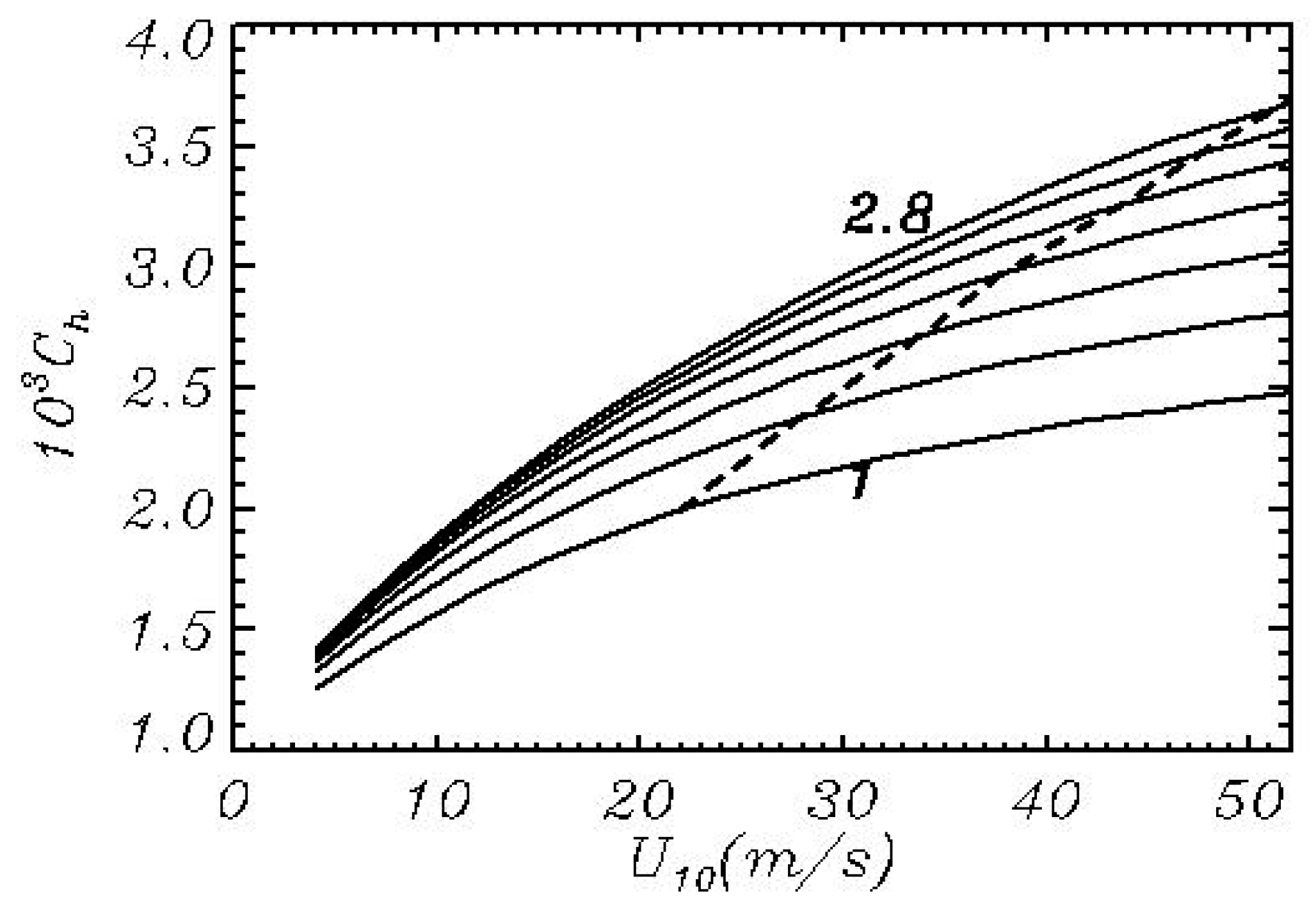
9. Thoughts on Drag Coefficient at Strong Wind
As demonstrated in Figure 12, the current theory predicts a monotonic growth of drag coefficient with an increase of wind speed. However, there exist some data revealing that for a wind speed exceeding 25–30 , the drag coefficient reaches an upper limit (Powell et al. 2003, Donelan et al. 2004), while as the wind speed increases further, the drag coefficient can decrease. Earlier such an effect was also noted when analyzing the tropical cyclone development (Emanuel, 1995). Currently, some attempts are made to explain such behavior of drag coefficient on the basis of a ‘droplet theory’ [43,62,63,64]. According to this theory, the drops generated as a result of the splitting of falling water volumes intensify the dissipation of turbulence, which causes reduction of drag coefficient. Such scheme looks reasonable, although a model of drop generation (as well as the mechanism of drops-turbulence interaction) uses too many arbitrary assumptions and ‘constants’, leaving a great possibility for fitting the theory to the observation data. In fact, this mechanics was suggested by Barenblatt and Golitsyn [65] for explanation of a dust storm phenomenon (and for liquid fuel droplets in rocket engines before that). According to their theory, sand particles increase the dissipation of turbulence and decrease friction, which accelerates the flow. The difference between the sea condition and desert is that the specific weight of sand particles is 3—4 times larger than that of water, and the concentration of sand particles is very high (visibility in dust storms is usually zero). It is easy to estimate that the density of sand fraction in a dust storm is by orders of magnitude higher than the density of water in a flow above sea waves.
According to our data, an effect of the wave-drag reduction at high wind speeds can be easily explained through the influence of high-frequency waves. As seen in Figure 10, about 50–70% of WPMF is transferred to waves at frequencies . Hence, the variation of stress in a high-frequency part of the spectrum can modify the drag coefficient. It would be appropriate to suggest that the energy of short waves at high winds decreases due to two factors: the presence of bubble foam that suppresses short waves, and the flow deceleration in troughs due to the flow separation. The latter can be investigated using the coupled wind-wave model directly, though the model must take into account a broad range of wave spectrum from peak waves to capillary waves. A high wind speed and the necessity to use a high vertical resolution in the WBL make this problem quite time-consuming; however, such calculations are possible from a technical point of view. Note that the reduction of drag can also be caused by ‘blowing away’ sharp crests: high winds can smooth the surface and remove the elements responsible for stress. This effect was directly observed in the wind-wave tunnel (J. Troitskaya—private communication).
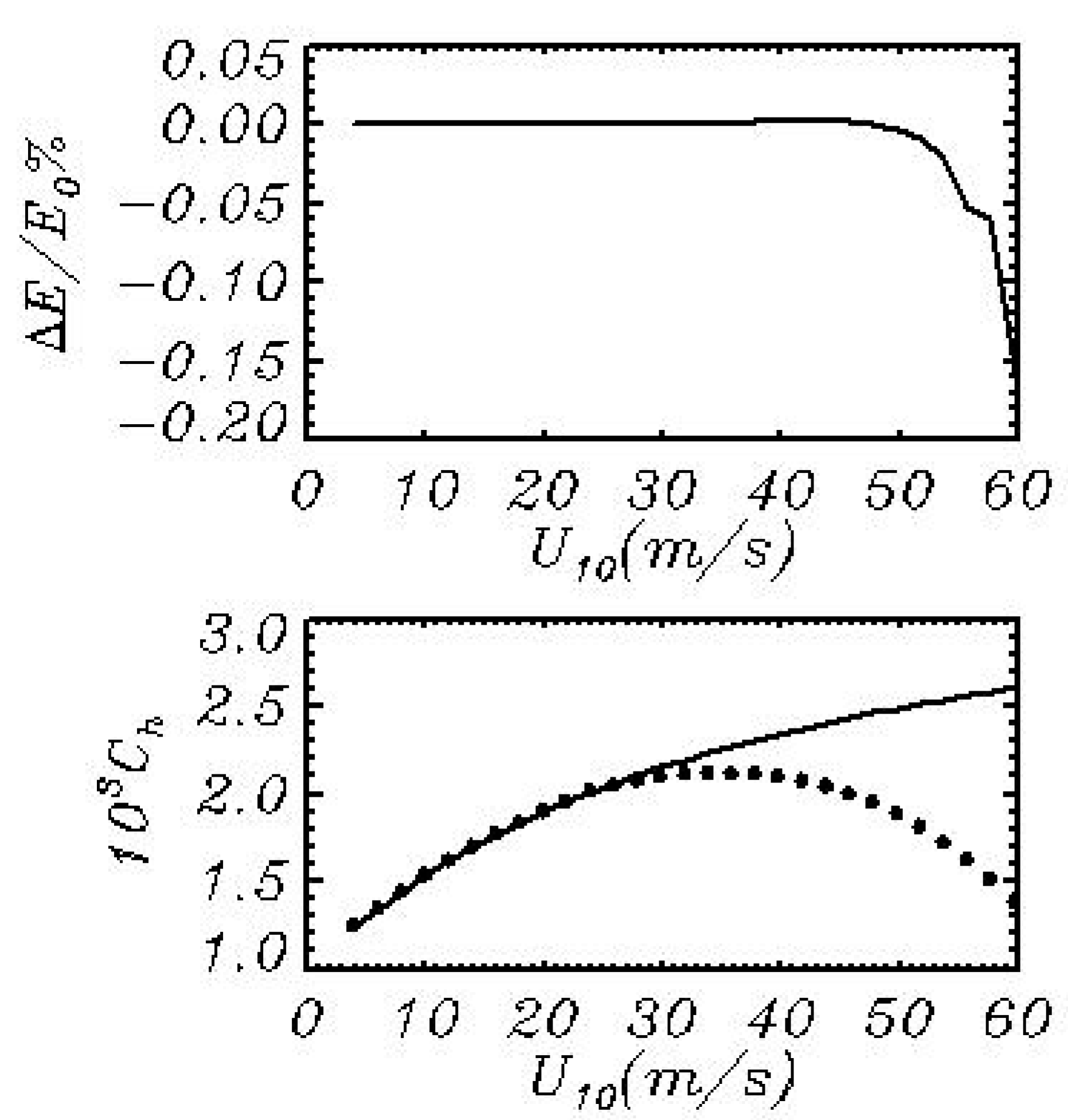
To prove that the reduction of drag coefficient is caused by the suppression of small waves, the additional calculations of drag coefficient were performed with a use of a non simplified WBL model described in Section 3 for the modified JONSWAP spectrum. A somewhat arbitrary assumption suggests that waves, whose frequency exceeds some value of , are absent. In other words, we just cut the spectral tail in small pieces starting from and calculated the stationary structure of the WBL and drag coefficient. The calculations were started from when a drag coefficient was equal to . Then the calculations were repeated for the next wind value, with cutting a new portion of wave tail. The sizes of cuts were chosen for good qualitative approximation of data obtained on [51,55,66]. The final dependence is shown by dots in the lower panel of Figure 17. In the upper panel a relative decline of total wave energy is shown. It is seen that a considerable decrease of drag can be reached by a very small reduction of energy in a high-frequency part of the spectrum. Note that the form of reduction does not influence general results: essentially the same dependence can be obtained by increase of the rate of energy drop in the spectral tail.
It should be emphasized that the result presented in Figure 17 is purely qualitative, since the exact shape of spectrum at high wind speeds is unknown. Figure 17 just illustrates a simple explanation of the drag coefficient reduction at high wind speeds on the basis of the high-frequency wave spectrum modification. To take into account this effect, it is necessary to study the exact shape of spectrum tail, i.e., to find a connection between the wind velocity and energy in a high-frequency part of spectrum. This problem seems to be simpler than defining a set of ‘constants’ in the equations of the ‘droplet’ theory.
10. Conclusions
Contrary to the turbulent transfer, the wave-produced momentum flux (WPMF) is not an internal factor of the wave boundary layer (WBL), since the structure and magnitude of the WPMF are controlled by the wave field. Only the stationary and horizontally homogeneous flow above smooth or rough surface has the universal structure. Even above land such conditions are seldom, because in reality the surface is inhomogeneous, and the external flow is nonstationary. Above sea the variable wind and advection of wave energy produce infinite diversity of wave spectra. The dynamic structure of wave boundary layer considered in this paper is completely defined by upper boundary conditions (i.e., wind velocity or turbulent stress) and wave field properties. This is true if the wind or wave spectrum does not change; otherwise the structure of the WBL depends on a relatively short prehistory. All these processes can be well simulated by coupling the WBL 2-D model or 3-D model with turbulence closure or LES schemes [67]—with the phase resolving model of waves (like the HOS model [68] or the finite difference model [69] or model [70].
Spectral wave models [14], as well as 2-D [17] and 3-D LES [21] modeling [67], or modeling with a turbulent closure scheme [17] require the parameterization of tangent stress and subgrid waves effects. The scheme (59–62) was developed specifically for these purposes. A more practical approach, such as wave prediction modeling [14] or coupled ocean-waves-atmosphere modeling [71] is based on a spectral presentation of wave fields. Parameterizations of the dynamic WBL should solve two main tasks: (1) calculate the flux of momentum lost by the atmosphere model and obtained by the ocean; (2) calculate the flux of energy to waves. Both of these problems are far from being resolved. Until recently numerous attempts have been made to find the best approximation for dependence of surface stress on wind velocity (see [72]). However, it became clear many years ago that such a unique dependence cannot exist (e.g., [73]). The drag coefficient at any given wind velocity is a product of the wave spectrum which can be quite different. For example, let us consider an ideal wave field consisting of one single mode. If wind direction coincides with the direction of wave propagation, the wave will produce some wave drag which is superimposed upon tangent drag. If the wave front is parallel to the wind direction, the wave-produced drag is equal to zero, and friction is supported by the tangent stress only. If the direction of the wind is the opposite to wave propagation, the drag will be larger than in the first case, because the rate of overflow is a sum of wind and phase velocities. In a multimode wave field, waves of different directions are present, but the effect of deviation of wave direction from the wind direction remains important (see Figure 16). Naturally, the magnitude and direction of wave drag strongly depends on thea shape of the two-dimensional wave spectrum .
Unfortunately, the data on wind vector and spectral shape cannot be converted directly into the magnitude of drag coefficient. For such purposes it is necessary to use a model of WBL that calculates the structure of the WBL and the rate of exchange by momentum and energy between wind and waves. The construction of the WBL model became possible following the investigation of function performed in [17] and the recent new post-processing of their results. For approximation (12), (13) of -function 1,400,000 individual values in the range of were used. The data on at had a large scatter and were considered as not quite reliable. Such values of are used infrequently. -function was defined by the processing of the simultaneous local values of elevation and surface pressure. The pressure was calculated by a standard method based on the Poisson equation, and to some degree can be considered as exact. However, the results depend on the vertical and horizontal resolution of WBL, and the significance of this dependence is not clear enough. We were not able check the effect of this resolution because the calculations similar to those described in [17] normally take several months. Note that the entire approach demonstrated in the current paper requires further investigation of -function calculated with a high-resolution coupled model. This problem is far from being solved; the current paper is just a first step in this direction.
The simplest way of derivation of the 1-D WBL model (Equations (21) and (23)) should be based on the complete Euler equations extended by an appropriate closure scheme. The averaging of the equation for horizontal momentum gives a 1-D equation that contains the components of WPMF. The vertical profiles of these components can be represented in a convenient form as a sum of fluxes produced by separate wave modes (see Figure 5). Finally, we obtain the equations which directly connect the structure of the WBL with an arbitrary wave spectrum. To avoid uncertainty with a lower boundary condition we used a very high resolution for frequency and height, which allowed us placing the lowest layer in a viscous sub-layer and calculate the tangent stress in the near-surface layer with the usage of molecular viscosity. The calculations showed that the results are not too sensitive to resolution. As an example, the solution of equations was done for the symmetrical JONSWAP spectrum. The structure of the WBL was illustrated by profiles of wind velocity and WPMF, as well as by energy of turbulence and some other characteristics. It is shown that the Charnock’s scaling decreases the dependence on wind velocity, but the coefficient in this formula still remains dependent on wind velocity and wave age. Finally, the dependence of drag coefficient on wind velocity and wave age was presented. Naturally, this result is valid only for the situations which are similar to the idealized conditions of the JONSWAP experiment. In reality, the general direction of the wind wave spectrum deviates from wind direction, and the spectrum can contain the waves not generated by local wind. Each spectrum at given velocity generates its own drag coefficient. If the conditions change quickly, the structure of WBL is not stationary, and the drag coefficient is not fully defined by the local spectrum and wind.
A detailed model that uses high resolution over wave frequency and elevation above the water surface cannot be used as an element of a complicated system similar to the wave prediction model or coupled ocean-atmosphere model. However, this model can be used for the development of a simplified approach which does not require considerable computational resources. The simplification of the model can be done by the sharp reduction of frequency range (engineering models like WAM or WAVEWATCH do not consider high-frequency waves). Parameterization is based on the evident properties of small waves: they are mostly generated by current wind; hence, their structure is more or less universal. We assume that an asymptotic form of wave spectrum at high frequencies is similar to that of the JONSWAP spectrum. It was shown before that the friction generated by subgrid waves and tangent stress can be parameterized in terms of cut-frequency, external friction velocity and wave age. The calculations of the WBL structure with a simplified model proved that such parameterization is acceptable.
The 1-D model of WBL is useful for the investigation of a broad range of problems. The main advantage of the model is a direct connection of the WBL structure with an arbitrary wave spectrum. In general cases, the WBL problem is nonstationary: the boundary layer is all the time adjusting to the changing wave field and wind velocity. If the model is used as a link in the atmosphere-waves-upper ocean system, the stationary solution is not always reachable, since the boundary conditions are typically unsteady.
This paper is devoted to the purely-dynamic interaction. The model will be generalized by including stratification effects and the equations for temperature and vapor transfer.
Author Contributions
Conceptualization—A.V.B.; Writing—original draft, D.C.; Writing review & editing, A.V.B.
Funding
This research received no external funding.
Acknowledgments
The current investigations presented in Section 2, Section 3, Section 4, Section 5 and Section 6 of paper is supported by RFBR (project №18-05-01122) and the Section 1, Section 7, Section 8 and Section 9 by state program 0149-2019-0015 (D. Chalikov). A.V. Babanin acknowledges support from the US Office of Naval Research grant N00014-17-1-3021.
Conflicts of Interest
The authors declare no conflict of interests.
References
- Charnock, H. Wind stress on a water surface. Quart. J. Roy. Meteorol. Soc. 1955, 81, 639–640. [Google Scholar] [CrossRef]
- Ursell, F. Wave generation by wind. In Surveys in Mechanics; Batchelor, G.K., Ed.; Cambridge University Press: Cambridge, UK, 1956; pp. 216–249. [Google Scholar]
- Miles, J.W. On the generation of surface waves by shear flows. J. Fluid Mech. 1957, 3, 185–204. [Google Scholar] [CrossRef]
- Phillips, O.M. Dynamics of Upper Ocean, 2nd ed.; Cambridge University Press: Cambridge, UK, 1977; p. 336. [Google Scholar]
- Chalikov, D.V. A mathematical model of wind–induced waves. Doklady Acad. Sci. USSR. 1976, 229, 121–126. [Google Scholar]
- Chalikov, D.V. Numerical simulation of wind–wave interaction. J Fluid Mech. 1978, 87, 561–582. [Google Scholar] [CrossRef]
- Chalikov, D.V. Mathematical modeling of wind waves. In Gidrometeoizdat Saint-Petersburg; 1980; 50p. [Google Scholar]
- Chalikov, D.V. Numerical simulation of the boundary layer above waves. Bound. Layer Met. 1986, 34, 63–98. [Google Scholar] [CrossRef]
- Chalikov, D. The parameterization of the wave boundary layer. J. Phys. Oceanogr. 1995, 25, 1335–1349. [Google Scholar] [CrossRef]
- Voermans, J.J.H.; Rapizo, H.; Ma, F.; Qiao, A.V. Babanin, Air-sea momentum fluxes during Tropical Cyclone Olwyn. J. Phys. Oceanogr. 2019. [Google Scholar] [CrossRef]
- Monin, A.S.; Yaglom, A.M. Statistical Fluid Mechanics: Mechanics of Turbulence; MIT Press: Cambridge, MA, USA, 1971; p. 769. [Google Scholar]
- Gent, P.R.; Taylor, P.A. A numerical model of the air flow above water waves. J. Fluid Mech. 1976, 77, 105–128. [Google Scholar] [CrossRef]
- Tolman, H.; Chalikov, D. On the source terms in a third-generation wind wave model. J. Phys. Oceanogr. 1996, 11, 2497–2518. [Google Scholar] [CrossRef]
- Tolman, H.L. The WAVEWATCH III °R Development Group: User Manual and System Documentation of WAVEWATCH III °R Version 4.18; Contribution No. 316; Environmental Modeling Center Marine Modeling and Analysis Branch: College Park, MA, USA, 2014. [Google Scholar]
- Chalikov, D.; Sheinin, D. Direct Modeling of One-dimensional Nonlinear Potential Waves. Nonlinear Ocean Waves. Adv. Fluid Mech. 1998, 17, 207–258. [Google Scholar]
- Chalikov, D. Interactive modeling of surface waves and boundary layer. In Ocean Wave Measurements and Analysis; Proceedings of the on the third Intern. Symp. WAVES 97, Virginia Beach, VA, USA, 3–7 November 1998; ASCE: Reston, VA, USA, 1998; pp. 1525–1540. [Google Scholar]
- Chalikov, D.; Rainchik, S. Coupled numerical modeling of wind and waves and the theory of the wave boundary layer. Boundary-Layer Meteorol. 2010, 138, 1–41. [Google Scholar] [CrossRef]
- Chalikov, D. Numerical Modeling of Sea Waves; Springer: Berlin/Heidelberg, Germany, 2016; p. 330. [Google Scholar]
- Sullivan, P.P.; McWilliams, J.C.; Moeng, C.-H. Simulation of turbulent flow over idealized water waves. J. Fluid Mech. 2000, 404, 47–85. [Google Scholar] [CrossRef] [Green Version]
- Sullivan, P.P.; Edson, J.B.; Hristov, T.; McWilliams, J.C. Large-eddy simulations and observations of atmospheric marine boundary layers above nonequilibrium surface waves. J. Atmos. Sci. 2008, 65, 1225–1245. [Google Scholar] [CrossRef]
- Sullivan, P.P.; McWilliams, J.C.; Oatton, E.G. Large-Eddy Simulation of Marine Atmospheric Boundary Layers above a Spectrum of Moving Waves. J. Atmos. Sci. 2014, 71, 4001–4027. [Google Scholar] [CrossRef] [Green Version]
- Yang, D.; Shen, L. Direct-simulation-based study of turbulent flow over various waving boundaries. J. Fluid Mech. 2010, 650, 131–180. [Google Scholar] [CrossRef] [Green Version]
- Yang, D.; Meneveau, C.; Shen, L. Dynamic modelling of sea-surface roughness for large eddy simulation of wind over ocean wavefield. J. Fluid Mech. 2013, 726, 62–99. [Google Scholar] [CrossRef]
- Richter, D.H.; Sullivan, P.P. Sea surface drag and the role of spray. Geophys. Res. Lett. 2013, 40, 656–660. [Google Scholar] [CrossRef] [Green Version]
- Miles, J.W. On the generation of surface waves by shear flows, Part 2. J. Fluid Mech. 1959, 6, 568–582. [Google Scholar] [CrossRef]
- Miles, J.W. On the generation of surface waves by turbulent shear flows. J. Fluid Mech. 1960, 7, 469–478. [Google Scholar] [CrossRef]
- Janssen, P.A.E.M. Quasi-linear theory of wind-wave generation applied to wave forecasting. J. Phys. Oceanogr. 1991, 21, 1631–1642. [Google Scholar] [CrossRef]
- Kudryavtsev, R.L.; Makin, V.K. The impact of air-flow separation on the drag of the sea surface. Boundary-Layer Meteorol. 2001, 98, 155–171. [Google Scholar] [CrossRef]
- Snyder, R.L.; Dobson, F.W.; Elliott, J.A.; Long, R.B. Array measurements of atmospheric pressure fluctuations above surface gravity waves. J. Fluid Mech. 1981, 102, 1–59. [Google Scholar] [CrossRef]
- Hsiao, S.V.; Shemdin, O.H. Measurements of wind velocity and pressure with a wave follower during MARSEN. J. Geophys. Res. 1993, 88, 9841–9849. [Google Scholar] [CrossRef]
- Hasselmann, D.; Bösenberg, J. Field measurements of wave-induced pressure over wind-sea and swell. J. Fluid Mech. 1991, 30, 391–428. [Google Scholar] [CrossRef]
- Donelan, M.A.; Babanin, A.V.; Young, I.R.; Banner, M.L.; McCormick, C. Wave follower field measurements of the wind input spectral function. Part, I. Measurements and calibrations. J. Atmos. Ocean. Technol. 2005, 22, 799–813. [Google Scholar] [CrossRef]
- Donelan, M.A.; Babanin, A.V.; Young, I.R.; Banner, M.L. Wave follower field measurements of the wind input spectral function. Part II. Parameterization of the wind input. J. Phys. Oceanogr. 2006, 36, 1672–1688. [Google Scholar] [CrossRef]
- Rogers, W.E.; Babanin, A.V.; Wang, D.W. Observation-consistent input and whitecapping-dissipation in a model for wind-generated surface waves: Description and simple calculations. J. Atmos. Ocean. Technol. 2012, 29, 1329–1346. [Google Scholar] [CrossRef]
- Liu, Q.; Rogers, W.E.; Babanin, A.V.; Young, I.R.; Romero, L.; Zieger, S.; Qiao, F.; Changlong, G. Observation-Based Source Terms in the Third-Generation Wave Model WAVEWATCH III: Updates and Verification. J. Phys. Oceanogr. 2019, 49, 489–517. [Google Scholar] [CrossRef]
- Plant, W.J. A relationship between wind stress and wave slope. J. Geophys. Res. 1982, 87, 1961–1967. [Google Scholar] [CrossRef]
- Donelan, M.A. Wind-induced growth and attenuation of laboratory waves. In Wind-Over-Wave Couplings. Perspective and Prospects; Sajadi, S.G., Thomas, N.H., Hunt, J.C.R., Eds.; Clarendon Press: Boston, MA, USA, 1999; pp. 183–194. [Google Scholar]
- Al’Zanaidi, M.A.; Hui, H.W. Turbulent airflow over water waves-a numerical study. J. Fluid Mech. 1984, 148, 225–246. [Google Scholar] [CrossRef]
- Chalikov, D.; Makin, V. Models of the wave boundary layer. Bound. Layer Met. 1991, 56, 83–99. [Google Scholar] [CrossRef]
- Chalikov, D.; Belevich, M. One–dimensional theory of the wave boundary layer. Bound. Layer Meteorol. 1993, 63, 65–96. [Google Scholar] [CrossRef]
- Mastenbroek, C.; Makin, V.K.; Garat, M.H.; Giovanangeli, J.P. Experimental evidence of the rapid distortion of turbulence in the air flow over water waves. J. Fluid Mech. 1996, 318, 273–302. [Google Scholar] [CrossRef]
- Chalikov, D.; Babanin, A.V. Nonlinear sharpening during superposition of surface waves. Ocean Dyn. 2016, 66, 931–937. [Google Scholar] [CrossRef]
- Troitskaya, Y.; Ezhova, E.; Irina Soustova, I.; Zilitinkevich, S. On the effect of sea spray on the aerodynamic surface drag under severe winds. Ocean Dyn. 2016, 66, 659–669. [Google Scholar] [CrossRef]
- Chalikov, D. Statistical properties of nonlinear one-dimensional wave fields. Nonlinear Process. Geophys. 2005, 12, 1–19. [Google Scholar] [CrossRef]
- Hasselmann, K.; Barnett, T.P.; Bouws, E.; Carlson, H.; Cartwright, D.E.; Enke, K.; Ewing, J.A.; Gienapp, H.; Hasselmann, D.E.; Kruseman, P.; et al. Measurements of wind-wave growth and swell decay during the Joint Sea Wave Project (JONSWAP). Deut. Hydrogr. Z. 1973, 8, 1–95. [Google Scholar]
- Babanin, A.V.; Soloviev, Y.P. Field investigation of transformation of the wind wave frequency spectrum with fetch and the stage of development. J. Phys. Oceanogr. 1998, 28, 563–576. [Google Scholar] [CrossRef]
- Thomas, L.H. Elliptic Problems in Linear Differential Equations over a Network; Columbia University: New York, NY, USA, 1949. [Google Scholar]
- Ocampo-Torres, F.J.; Donelan, M.A.; Merzi, N.; Jia, F. Laboratory measurements of mass transfer of carbon dioxide and water vapor for smooth and rough ow conditions. Tellus 1994, B46, 16–32. [Google Scholar] [CrossRef]
- Donelan, M.A.; Haus, B.K.; Reul, N.; Plant, W.J.; Stiassnie, M.; Graber, H.C.; Brown, O.B.; Saltzman, E.S. On the limiting aerodynamic roughness of the ocean in very strong wind. Geophys. Res. Lett. 2004, 31, L18306. [Google Scholar] [CrossRef]
- Large, W.G.; Pond, S. Open ocean momentum ux measurements in moderate to strong winds. J. Phys. Oceanogr. 1981, 11, 324–336. [Google Scholar] [CrossRef]
- Powell, M.D.; Vickery, P.J.; Reinhold, T.A. Reduced drag coefficient for high wind speeds in tropical cyclones. Nature 2003, 422, 279–283. [Google Scholar] [CrossRef] [PubMed]
- Jarosz, E.; Mitchell, D.A.; Wang, D.W.; Teague, W.J. Bottomup determination of air-sea momentum exchange under a major tropical cyclone. Science 2007, 315, 1707–1709. [Google Scholar] [CrossRef] [PubMed]
- Fernandez, D.E.; Carswell, J.R.; Frasier, S.; Chang, P.S.; Black, P.G.; Marks, F.D. Dualpolarized C- and Ku-band ocean backscatter response to hurricane-force winds. J. Geophys. Res. 2006, 111, C08013. [Google Scholar] [CrossRef]
- Bryant, K.M.; Akbar, M. An exploration of wind stress calculation techniques in hurricane storm surge modeling. J. Mar. Sci. Eng. 2016, 58. [Google Scholar] [CrossRef]
- Holthuijsen, L.H.; Powell, M.D.; Pietrzak, J.D. Pietrzak Wind and waves in extreme hurricanes. J. Geophys. Res. 2012, 117, C09003. [Google Scholar] [CrossRef]
- Moon, I.-J.; Isaac, G.; Tetsu, H. Effect of surface waves on air-sea momentum exchange. Part II: Behavior of drag coefficient under tropical cyclones. J. Atmos. Sci. 2004, 61, 2334–2348. [Google Scholar] [CrossRef]
- Walsh, K.J.; Sandery, P.; Brassington, G.B.; Entel, M.; Siegenthaler-LeDrian, C.; Kepert, J.D.; Darbyshire, R. Darbyshire Constraints on drag and exchange coeffcients at extreme wind speeds. J. Geophys. Res. 2019, 115, C09007. [Google Scholar]
- Zweers, N.C.; Makin, V.K.; de Vries, J.W.; Burgers, G. A sea drag relation for hurricane wind speeds. Geophys. Res. Lett. 2010, 37, L21811. [Google Scholar] [CrossRef]
- Zweers, N.C.; Makin, V.K.; de Vries, J.W.; Burgers, G. On the influence of changes in the drag relation on surface wind speeds and storm surge forecasts. Nat. Hazards 2012, 62, 207–219. [Google Scholar] [CrossRef]
- Vatvani, D.; Zweers, N.C.; van Ormondt, M.; Smal, A.J.; de Vries, H.; Makin, V.K. Storm surge and wave simulations in the Gulf of Mexico using a consistent drag relation for atmospheric and storm surge models. Nat. Hazards Earth Syst. Sci. 2012, 12, 2399–2410. [Google Scholar] [CrossRef]
- Zijlema, M.; van Vledder, G.P.; Holthuijsen, L.H. Bottom friction and wind drag for wave models. Coast. Eng. 2012, 65, 19–26. [Google Scholar] [CrossRef]
- Andreas, E.L. Spray-mediated enthalpy flux to the atmosphere and salt flux to the ocean in high winds. J. Phys. Oceanogr. 2010, 40, 608–619. [Google Scholar] [CrossRef]
- Kudryavtsev, V.N. On the effect of sea drops on the atmospheric boundary layer. J. Geophys. Res. 2006, 111, C07020. [Google Scholar] [CrossRef]
- Kudryavtsev, V.N.; Makin, V.K. Impact of ocean spray on the dynamics of the marine atmospheric boundary layer. Boundary-Layer Meteorol. 2011, 140, 383–410. [Google Scholar] [CrossRef]
- Barenblatt, G.I.; Golitsyn, G.S. Local Structure of Developed Dust Storms; Moscow State University: Moscow, Russia, 1973; p. 44. [Google Scholar]
- Zhang, L.; Oey, L. An Observational Analysis of Ocean Surface Waves in Tropical Cyclones in the Western North Pacific Ocean. JGR Oceans 2019, 124, 184–195. [Google Scholar] [CrossRef]
- Sullivan, P.P.; McWilliams, J.C. Dynamics of Winds and Currents Coupled to Surface Waves. Annu. Rev. Fluid Mech. 2010, 42, 19–42. [Google Scholar] [CrossRef] [Green Version]
- Ducrozet, G.; Bonnefoy, F.; Le Touzé, D.; Ferrant, P. HOS-ocean. Open-source solver for nonlinear waves in open ocean based on High-Order Spectral method. Comp. Phys. Commun. 2016. [Google Scholar] [CrossRef]
- Engsig-Karup, A.P.; Harry, B.; Bingham, H.B.; Lindberg, O. An efficient flexible-order model for 3D nonlinear water waves. J. Comput. Phys. 2009, 228, 2100–2118. [Google Scholar] [CrossRef]
- Chalikov, D.; Babanin, A.V.; Sanina, E. Numerical Modeling of Three-Dimensional Fully Nonlinear PotentialPeriodic Waves. Ocean Dyn. 2014, 64, 1469–1486. [Google Scholar] [CrossRef]
- Warner, J.C.; Armstrong, B.; He, R.; Zambon, J.B. Development of a Coupled Ocean–Atmosphere–Wave–Sediment Transport (COAWST) Modeling System. Ocean Model. 2010, 35, 230–244. [Google Scholar] [CrossRef]
- Sterl, A. Drag at high wind velocities—A review. Roy. Netherland Met. Office. Tech. Rep. 2017, 361, 23. [Google Scholar]
- Babanin, A.V.; Makin, V.K. Effects of wind trend and gustiness on the sea drag: Lake George study. J. Geophys. Res. 2008, 113, C02015. [Google Scholar] [CrossRef]
Figure 1.
Shape of as a function of nondimensional frequency . The filled areas characterize uncertainty of approximation. 1—Snyder [29] (red color in the interval (0–2.5); 2—Plant [36]; 3—Hasselmann and Bösenberg [31]; 4—Donelan [32,33]; 5—Hsiao [30]; 6—Donelan [37]; 7—Chalikov, Rainchik [17].

Figure 2.
A typical snapshot of tracers in the WBL above waves. The picture is seven times stretched in a vertical direction.
Figure 2.
A typical snapshot of tracers in the WBL above waves. The picture is seven times stretched in a vertical direction.

Figure 3.
The values the of imaginary (1) and real (2) parts of -function calculated with (10) and (11). Inset shows the imaginary part of -function in vicinity of 0.
Figure 3.
The values the of imaginary (1) and real (2) parts of -function calculated with (10) and (11). Inset shows the imaginary part of -function in vicinity of 0.

Figure 4.
Dependence of R on the nondimensional frequency . Function is given in Figure 4.
Figure 4.
Dependence of R on the nondimensional frequency . Function is given in Figure 4.

Figure 5.
Upper panel: vertical profiles of Fourier components of WPMF (Wave Produced Momentum Flux) as a function of height z. Bottom panel—the same profiles, but each being normalized by their surface values as a function of (Equations (19) and (20)).
Figure 5.
Upper panel: vertical profiles of Fourier components of WPMF (Wave Produced Momentum Flux) as a function of height z. Bottom panel—the same profiles, but each being normalized by their surface values as a function of (Equations (19) and (20)).

Figure 6.
Dependence of the significant wave height on wind velocity and inverse wave age : 1— = 1, 2—1.3; 3—1.6; 4—1.9; 5—2.2; 6—2.5 7—2.8. A horizontal dotted line separates the area of unrealistic values of
Figure 6.
Dependence of the significant wave height on wind velocity and inverse wave age : 1— = 1, 2—1.3; 3—1.6; 4—1.9; 5—2.2; 6—2.5 7—2.8. A horizontal dotted line separates the area of unrealistic values of

Figure 7.
The examples of wave profile for the values of 14, 22 and 30 m/s. Thick curves correspond to , while thin curves relate to .
Figure 7.
The examples of wave profile for the values of 14, 22 and 30 m/s. Thick curves correspond to , while thin curves relate to .

Figure 8.
The vertical profiles of turbulent momentum flux (solid curves) and WPMF (dashed curves), normalized by external momentum flux . Curves 1, 2 and 3 refer to for the wind velocity 14, 22 and 30 m/s, respectively; curves 4, 5 and 6 refer to for the same wind velocities. Thick curves correspond to , while thin curves to .

Figure 9.
The dependence of surface tangent stress (Equation (28)) normalized by the external value of stress on wind velocity and inverse wave age . Only edge values and are marked. The intermediate values of are indicated in a caption to Figure 5. On the right of a dotted curve is the area of unrealistic values of .

Figure 10.
The integral WPMF normalized by external stress as a function of , and : 1— 2—; 3— Solid curves correspond to ; dotted curve to dashed curves to .
Figure 10.
The integral WPMF normalized by external stress as a function of , and : 1— 2—; 3— Solid curves correspond to ; dotted curve to dashed curves to .

Figure 11.
The integral energy flux to waves normalized by the external energy flux at height as a function of and : 1— 2—; 3— Solid curves correspond to , a dotted curve correspond to dashed curves correspond to .
Figure 11.
The integral energy flux to waves normalized by the external energy flux at height as a function of and : 1— 2—; 3— Solid curves correspond to , a dotted curve correspond to dashed curves correspond to .

Figure 12.
Dependence of the total roughness parameter (Equation (1)) normalized by the Charnock scale as a function of wind velocity and inverse wave age . Only the edge values and are marked (see capture to Figure 8).
Figure 12.
Dependence of the total roughness parameter (Equation (1)) normalized by the Charnock scale as a function of wind velocity and inverse wave age . Only the edge values and are marked (see capture to Figure 8).

Figure 13.
Dependence of a drag coefficient as a function of wind velocity and inverse wave age . Only the edge values and are marked (see capture to Figure 9). A dashed curve separates the area of unrealistic waves.
Figure 13.
Dependence of a drag coefficient as a function of wind velocity and inverse wave age . Only the edge values and are marked (see capture to Figure 9). A dashed curve separates the area of unrealistic waves.

Figure 14.
Comparison of the subgrid stresses calculated by model and by Equations (59)–(62) . Left panel: comparison of the wave-produced surface stress obtained with a high-resolution wave model with approximations by Equations (59) and (60). Right panel: the same as in the left panel, but for the tangent stress and approximations by Equations (61) and (62).

Figure 15.
Dependence of drag coefficient on wind velocity for different angles between a general direction of waves and the wind direction : 1—; 2—; 3—; In each group thick curves correspond to , while a thinner curve to , and thin curves to .
Figure 15.
Dependence of drag coefficient on wind velocity for different angles between a general direction of waves and the wind direction : 1—; 2—; 3—; In each group thick curves correspond to , while a thinner curve to , and thin curves to .

Figure 16.
Dependence of drag coefficient on the angle between wind direction and general direction of waves for : 1—; 2—; 3—.
Figure 16.
Dependence of drag coefficient on the angle between wind direction and general direction of waves for : 1—; 2—; 3—.

Figure 17.
The influence of energy of the high-frequency part of spectrum on drag coefficient. In upper panel the reduction of wave energy (%) due to truncation of the spectral tail is shown. The bottom panel shows the undisturbed dependence of drag coefficient (solid curve) and a drag coefficient calculated at the truncated spectrum (dots).

© 2019 by the authors. Licensee MDPI, Basel, Switzerland. This article is an open access article distributed under the terms and conditions of the Creative Commons Attribution (CC BY) license (http://creativecommons.org/licenses/by/4.0/).
Share and Cite
MDPI and ACS Style
Chalikov, D.; Babanin, A.V. Parameterization of Wave Boundary Layer. Atmosphere 2019, 10, 686. https://doi.org/10.3390/atmos10110686
AMA Style
Chalikov D, Babanin AV. Parameterization of Wave Boundary Layer. Atmosphere. 2019; 10(11):686. https://doi.org/10.3390/atmos10110686
Chicago/Turabian StyleChalikov, Dmitry, and Alexander V. Babanin. 2019. "Parameterization of Wave Boundary Layer" Atmosphere 10, no. 11: 686. https://doi.org/10.3390/atmos10110686
Note that from the first issue of 2016, this journal uses article numbers instead of page numbers. See further details here.