Article

Atmospheric Trace Metal Deposition near the Great Barrier Reef, Australia

1
Institute for Marine and Antarctic Studies, University of Tasmania, Hobart TAS 7005, Australia
2
Australian Centre for Research on Separation Science, University of Tasmania, Hobart TAS 7005, Australia
3
Antarctic Climate and Ecosystems CRC, University of Tasmania, Hobart TAS 7005, Australia
4
School of Earth Sciences, University of Melbourne, Melbourne VIC 3010, Australia
5
ARC Centre of Excellence for Climate System Science, University of New South Wales, Sydney NSW 2052, Australia
6
International Laboratory for Air Quality and Health, Queensland University of Technology (QUT), Brisbane City QLD 4000, Australia
7
Climate Science Centre, Oceans and Atmosphere, CSIRO, 107-121 Station St, Aspendale VIC 3195, Australia
*
Author to whom correspondence should be addressed.
Atmosphere 2020, 11(4), 390; https://doi.org/10.3390/atmos11040390
Submission received: 19 March 2020 / Revised: 3 April 2020 / Accepted: 7 April 2020 / Published: 15 April 2020
(This article belongs to the Special Issue The Formation and Transformation of Atmospheric Soluble Iron)

Abstract

:
Aerosols deposited into the Great Barrier Reef (GBR) contain iron (Fe) and other trace metals, which may act as micronutrients or as toxins to this sensitive marine ecosystem. In this paper, we quantified the atmospheric deposition of Fe and investigated aerosol sources in Mission Beach (Queensland) next to the GBR. Leaching experiments were applied to distinguish pools of Fe with regard to its solubility. The labile Fe concentration in aerosols was 2.3–10.6 ng m−3, which is equivalent to 4.9%–11.4% of total Fe and was linked to combustion and biomass burning processes, while total Fe was dominated by crustal sources. A one-day precipitation event provided more soluble iron than the average dry deposition flux, 0.165 and 0.143 μmol m−2 day−1, respectively. Scanning Electron Microscopy indicated that alumina-silicates were the main carriers of total Fe and samples affected by combustion emissions were accompanied by regular round-shaped carbonaceous particulates. Collected aerosols contained significant amounts of Cd, Co, Cu, Mo, Mn, Pb, V, and Zn, which were mostly (47.5%–96.7%) in the labile form. In this study, we provide the first field data on the atmospheric delivery of Fe and other trace metals to the GBR and propose that this is an important delivery mechanism to this region.

1. Introduction

Oceans play an essential role in Earth’s climate through the uptake of atmospheric CO2. An important component of this system is the land-atmosphere-ocean transport of minerals and micronutrient trace elements vital to biology [1,2,3]. Included in this is the iron (Fe) biogeochemical cycle, in which Fe-rich aerosols are delivered to the oceans as a result of the deposition of mineral dust, biomass burning, and anthropogenic emissions. Trace micronutrients, such as Fe, are essential for the biogeochemical functioning of marine ecosystems [4,5,6]. The Great Barrier Reef (GBR) is an oligotrophic environment and, in general, a net source of CO2 to the atmosphere [7]. The GBR is an ecosystem on the verge of collapse due to climate change such as temperature increase and ocean acidification [8]. Phytoplankton growth in the temperate waters of the GBR is generally limited by nitrogen (N), which is provided by alluvial deposition from agricultural lands of northern Queensland in the summer-wet season (December–April) or through nitrogen fixation by cyanobacteria in the winter-dry season (May-September) [9]. The most common phytoplankton species in the GBR is the cyanobacteria Trichodesmium, which is characterised by high Fe requirements [10,11]. Consequently, during the winter-dry season, low atmospheric deposition of Fe may limit nitrogen fixation and, consequently, phytoplankton growth [12,13,14]. A distinct response in chlorophyll production to mineral dust deposition was observed along the GBR coast after a massive dust storm in 2002 [13,14]. On the other hand, for some dust events, the ocean biological response was difficult to confirm or was not observed [15,16]. Understanding atmospheric deposition of Fe and other trace metals (TMs) and their potential role in biogeochemical cycling in this region is limited. Atmospheric Fe deposition in oligotrophic waters such as the GBR may promote nitrogen fixation and, consequently, alter the carbon cycle [17,18,19,20].
Atmospheric aerosol deposition delivers potentially toxic elements to the sensitive GBR marine environment and to local habitats [21]. Atmospheric concentrations of lead (Pb) above accepted environmental standards were reported in the coastal city of Townsville near the GBR due to ore transport and marine port activities [22]. Other elements, such as copper (Cu), influence marine biota by inhibiting fertilization success during the mass coral spawning [23,24]. Deposition of Zn, which is commonly emitted by the shipping industry, has caused consumption of the coral’s metal detoxificator, in which dimethyl sulfoniopropionate influences long-term coral health [25].
A key challenge in studying the atmospheric deposition of nutrients to the oceans is the quantification of bioavailable nutrients that can be used for photosynthesis and other biochemical processes. Bioavailability depends, in part, on nutrient solubility in seawater. Therefore, a wide range of leaching experiments and digestion experiments have been applied to determine the amount and proportion of nutrients that may dissolve in a range of different leaching media. Results show a large range of observed atmospheric Fe solubility worldwide: 0.01%–80% [26]. In Australia, reported solubilities for aerosols collected on the coast are rather within the lower range: 0.6%–6.0% in Western Australia [27], 2%–12% in the Northern Territory [28], and 0.5%–56% in Tasmania [29]. The main types of aerosol sources are mineral dust, biomass burning, volcanic eruptions, and a variety of anthropogenic emissions including (among others) industrial and domestic combustion processes as well as shipping and road dust from tires and car brakes. The vast majority of total Fe in global aerosol budgets comes from mineral dust, where Fe is contained in a variety of minerals. However, the fraction of soluble Fe in mineral dust is low, below 1% for most Fe oxides and around 4% for most alumina-silicates [30]. In contrast, pyrogenic emissions provide little total Fe compared to mineral dust, but this Fe is more soluble and it has recently been suggested to have a dominant contribution to the soluble Fe pool in waters around Australia [31,32]. Desboeufs et al. [33] found that TMs in carbonaceous matrices (e.g., combustion products) are more soluble than in alumina-silicate crystal clusters. Desboeufs et al. [33] also reported that Fe solubility for oil fly ash (36%) was much higher than for coal fly ash (0.2%) and urban dust (3.0%). The high solubility of oil combustion products was confirmed by Schroth et al. [34] who reported Fe solubilities of up to 81%, while arid soils and glacial products had low solubilities (1% and 2%–3%, respectively). The contribution of soluble Fe to total Fe in mineral dust is often significantly higher at the place of deposition compared to the origin due to processes such as proton-promoted and ligand-promoted dissolution [35,36,37] and photochemical reactions [38,39,40]. Furthermore, mixing with acidic gases and particulates combined with condensation evaporation cloud cycles may induce significant pH variations and creates easily soluble amorphous Fe particles [41,42,43]. However, a study by Winton and co-authors showed that the solubility of Fe in mineral dust may still be low even after a long-distance transport [44].
The origin of total and soluble Fe in aerosols can be investigated by studying their correlation with other chemical markers. Each elemental marker may represent a distinct anthropogenic emission, e.g., V for oil combustion [45,46]. Levoglucosan (LG) is a marker of cellulose degradation and, consequently, biomass burning processes [47,48,49], which is similar to non-sea salt potassium (nss-K) [50,51], while black carbon (BC) represents emissions from both biomass burning and anthropogenic combustion processes [52]. Increases in Fe solubility were found to be correlated with biomass burning and combustion processes markers [34,46,53]. Elements found in biomass and anthropogenic combustion, non-sea salt potassium (nss-K) and V, have also been used to determine relationships with the soluble Fe content [46]. Siefeld et al. [54] observed a sporadic high fractional iron solubility (FFeS) defined as contribution of soluble forms of Fe in total Fe in aerosols collected in the Arabian Sea coinciding with the fine V fraction, which suggests possible influences from ship emissions. Anthropogenic emissions also contributed to the atmospheric deposition of soluble Fe [55], as indicated by correlations between FFeS and the content of Fe sulfates and Fe oxalates, as well as the presence of the fossil fuel marker V.
Additionally, enrichment factors (EF) can provide information about the enrichment of a chosen element in the atmosphere relative to the upper continental crust, and, consequently, provide information on whether crustal or anthropogenic activity is the primary source of the element. Aluminium (Al) and titanium (Ti) are commonly used as proxies for mineral dust for EF calculations as their concentrations in the upper continental crust are high and relatively constant on a global scale [56]. However, Mackie et al. [57] found that Al is more easily abraded from soil than Fe and questioned its application as a mineral aerosol proxy. Moreover, Al is also contained in soot materials [33,58,59], which makes it a less specific marker. Therefore, Ti is likely a more reliable mineral dust proxy for aerosol samples.
The aim of this study was to quantify atmospheric trace metal (TM) concentrations and solubilities for the sensitive GBR region. In addition to Fe, we also analysed the fractional solubility of other elements that are considered important marine bioactive TMs including coral toxins (Cu, Pb, Zn), widely scrutinized elements (Cd, Mn, Mo,) and other potential nutrients (Co, V) [60,61,62]. We also aimed to fingerprint the sources of TMs and their contribution to FFeS as toxins. We, therefore, analysed TM concentrations and solubilities in aerosol and rainwater samples collected at Mission Beach, Queensland, in the vicinity of the GBR. We applied a three-stage leaching protocol, consisting of (i) a ultra-high purity water (UPW) leach-through, (ii) an ammonium acetate (pH 4.7) buffer bath, and (iii) a total digestion to determine the soluble, leachable, and refractory fractions of bioactive trace elements, respectively [3]. We studied the sample origin using air-mass backward trajectories (BT) and wind direction records from a local weather station. We applied EF analysis to distinguish between crustal and anthropogenic origin of elements and investigated the relationship between FFeS and biomass burning and combustion in general using the indicators LG and BC, respectively. The influence of soluble major ions (MI) and oxalate on FFeS was studied to investigate the aging processes and combustion source influences. Lastly, representative samples were analysed by Scanning Electron Microscopy (SEM) to identify the main elemental composition of Fe-bearing particulates.

2. Experiments

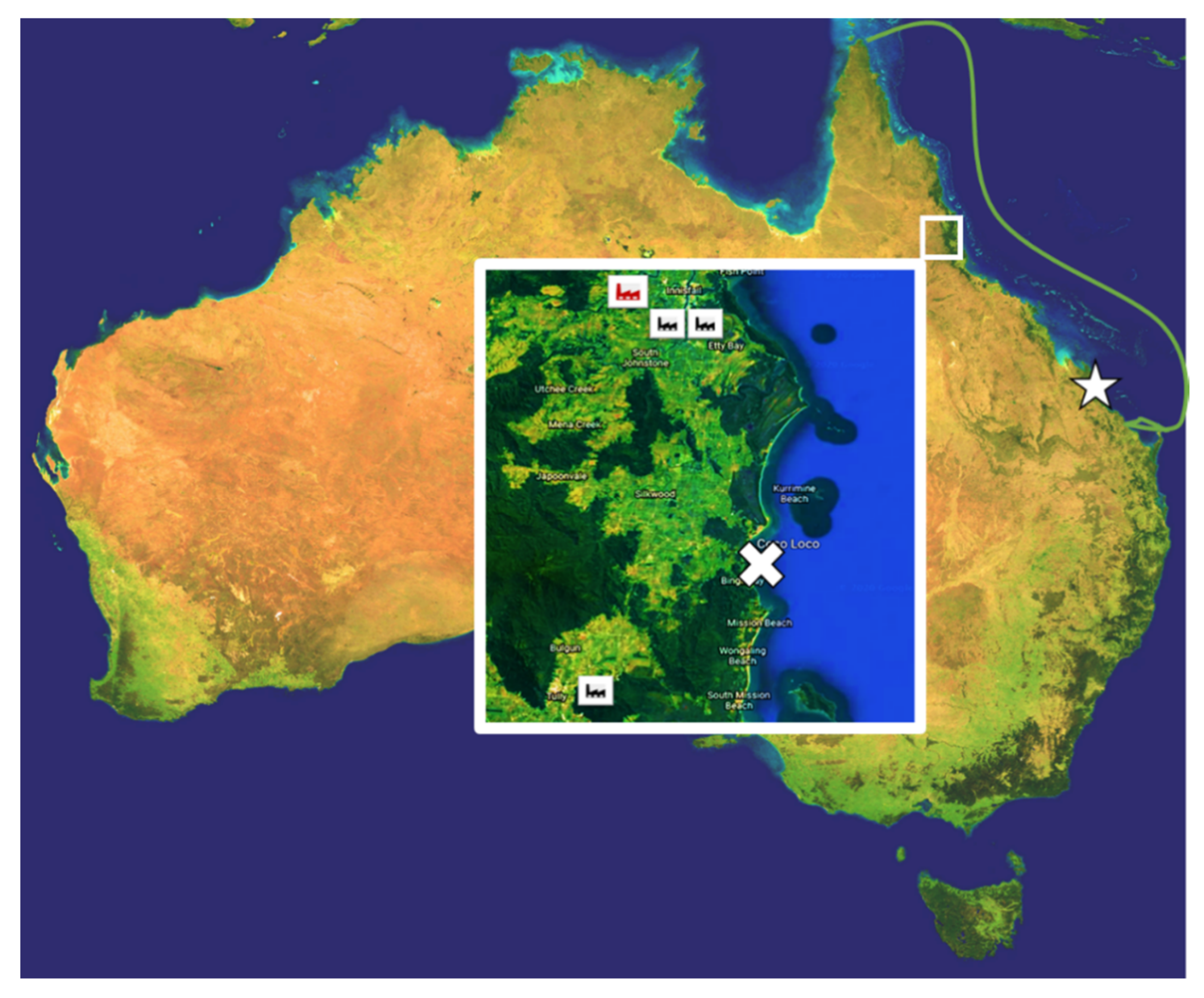
2.1. Sample Collection

Aerosol and rain samples were collected during the ‘Reef to Rainforest’ campaign [63,64], which used facilities of the Atmospheric Integrated Research on Burdens and Oxidative capacity (AIRBOX) project [65] to study atmospheric properties in Mission Beach, Queensland (Australia). A mobile air laboratory, AIRBOX, was located in direct proximity to the coastline and the GBR, around 150 km south-east of Cairns in the Coco Loco recreation resort (17.82° S, 146.12° E) (Figure 1), was surrounded by tropical rain forests and agricultural areas. To differentiate between aerosols transported from the sea during the day and those transported from the land at night, a short 12-h sampling period was applied from 6 a.m.–6 p.m. and 6 p.m.–6 a.m. (the first three samples were collected for 24 h). The sampling campaign was from 17 September to 7 October 2016, but samples chosen for analysis were collected between 19 September and 5 October 2016. Detailed information about sampling periods are given in Table S1. A high-volume air sampler, HiVol3000 (Ecotech), was placed on the roof of the AIRBOX container (Figure 1), and the sampling height was ~25 m above sea level. Aerosol particulates were accumulated by pumping the air through an acid-cleaned full sheet (20 cm x 25 cm) cellulose filter (Whatman 41, W41) without a size cut-off (TSP). As a result, we directly measured concentrations of trace metals in air, and use these data to estimate trace metal deposition fluxes using the methods previously described [28,66,67,68]. Before sampling, filters were cleaned for TM analysis according to GEOTRACES procedures [69,70]. After sampling, aerosol laden filters were folded in half (aerosol layer inside) and stored until analysis in two zip lock plastic bags in the freezer. There was no TM clean laboratory available in the field. Instead, all filter preparation and handling in the field was done inside an in-house made simple box consisting of plastic pipes covered by plastic sheeting without the high-efficiency particulate air (HEPA) filter air flow (Appendix A) that was regularly cleaned with UPW. Contamination issues were investigated by blank samples analysis (Appendix A) to assess the contamination provided by in-field sample handling. Before analysis, in the clean laboratory, two 47-mm diameter subsamples of the full filter sheet were taken using a pre-cleaned circular Ti punch and one was used for leaching and digestion experiments while the second subsample was used for major ion analysis.
Rainwater samples were collected on the top of the AIRBOX container roof using an in-house made rain sampler. An HDPE funnel and collection bottle (LDPE) for rainwater were cleaned according to GEOTRACES protocols [70]. Sample bottles were capped and stored in double plastic bags in the freezer until analysis. Two rain samples were collected over the entire campaign and then analyzed for trace element concentrations. Both were collected on 22 September 2016 (local time). The rain water sampler was exposed at the beginning of the rain event and deployed until several minutes after the end of the rain event. Sampling times were 165 and 135 min for the first and second rain event, respectively. The first rain event was a heavy rainfall for which the amount of collected water exceeded the sampler capacity (>500 mL, exceeding 5 mm of rainfall in the event). The second rain event was a shower and provided about 1 mm of rainfall (~100 mL). Our results revealed three fractions of Fe contained in rain water: (1) soluble, defined as the fraction passing through a W41 filter, (2) total-dissolvable, defined as the difference between being suspended in the non-filtered and filtered sample before solution acidification, and (3) particulate, defined as the digest of the fraction remaining on the filter. The same type of filter was applied for rain water filtration, which was used for dry deposition collection leaching experiments (cleaned W41). The relative contribution of Fe fractions was similar for both samples. The amount of Fe deposited on the surface area unit, called Fe wet deposition flux (Fwet), was calculated based on the funnel inlet area size, volume of collected water, and Fe concentration (1).
Fwet = [Fe]rain × Vrain/Ainlet
where: [Fe]rain is a concentration of chosen fraction of Fe (soluble, suspended, and particulate) in collected rain water, Vrain is a volume of collected rain water, and Ainlet is a surface area of the funnel inlet.

2.2. Back Trajectories Analysis

To distinguish remote aerosol sources and investigate air masses transport paths, samples were classified, according to their origin using back trajectories (BT) obtained from NOAA Air Resources Laboratory Hybrid Single-Particle Lagrangian Integrated Trajectory (HYPSPLIT) and the Global Data Assimilation System (GDAS) 05 model, with 3-h intervals and 72-h BT periods (Figure S1) [72,73]. The shorter interval allowed us to assess the homogeneity of the air masses. The height of the sampler location of 25 m above sea level was applied for generating backward trajectories. Based on these BTs, samples were divided into the following groups: marine (samples MB3, MB4, MB5, MB6, MB7, MB9, MB10) and terrestrial (samples MB11, MB12, MB13, MB18A, MB18, MB20). The remaining samples represent either mixed sources (MB19) or terrestrial aerosols, which were transported over the sea and returned to the coast (MB17, MB23, MB24, MB25) (Table S2).

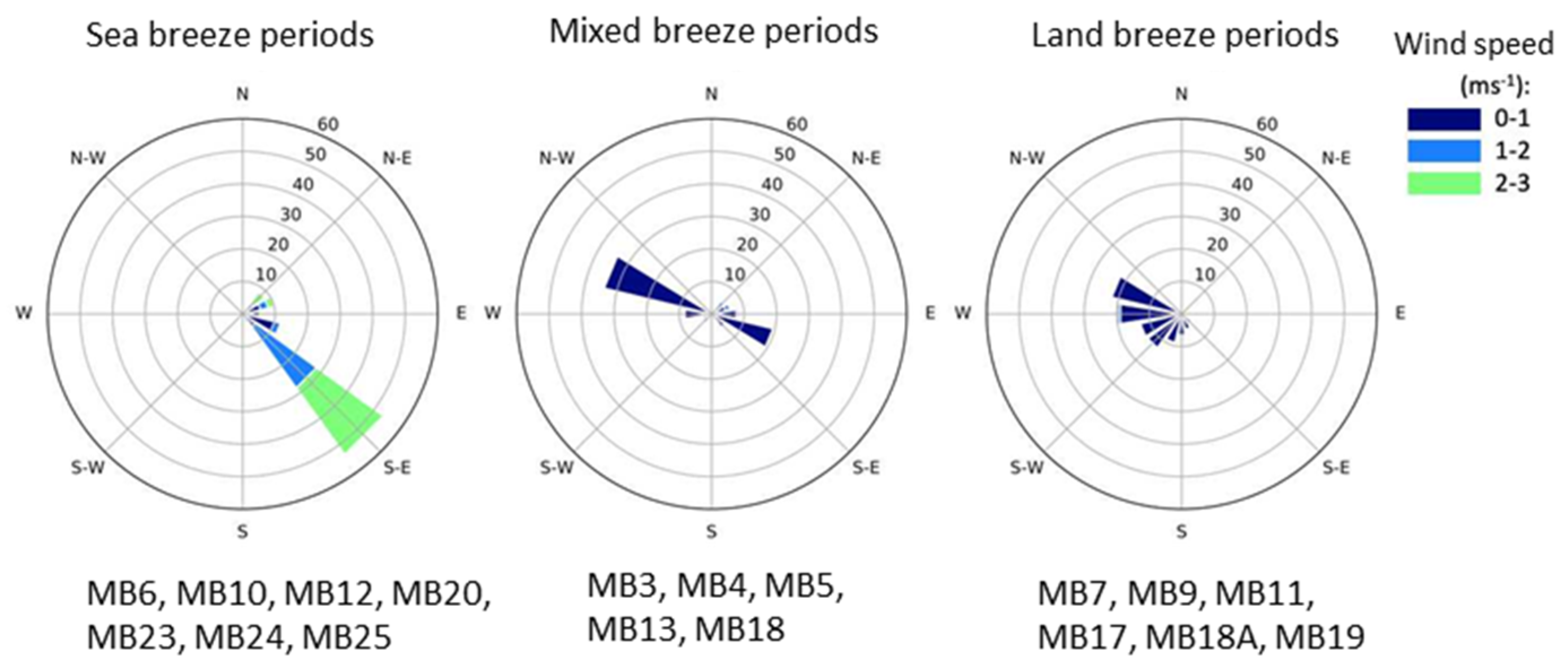
2.3. Wind Direction Analysis

In addition to back trajectories, samples were classified according to the wind patterns to consider contribution of local sources. Wind data was recorded by a Thompson WS800 Meteorological Station located on the top of AIRBOX container, approximately two meters from the aerosol sampler. Samples were classified into three groups based on the dominating wind direction (Figure 2): sea breeze (samples MB6, MB10, MB12, MB20, MB23, MB24, MB25), land breeze (samples MB7, MB9, MB11, MB17, MB18A, MB19), and mixed breeze (samples MB3, MB4, MB5, MB13, MB18).

2.4. Aerosol Sample Preparation

Samples collected on 47-mm filter punches were subjected to a three-step analytical protocol described by Perron et al. [3] and then analysed by Inductively Coupled Plasma Mass Spectrometry (ICP-MS) using a similar instrument setup as that reported in Bowie et al. [74]. Briefly, the protocol consists of three consecutive steps using the same 47-mm filter punch in each step. Step 1, ultra-pure water (UPW) leach: The subsample was put into Savillex Perfluoroalkoxy (PFA) filter holder and 50 mL of UPW was passed through the filter using a vacuum pump and collected in a Teflon container. An aliquot of the UPW leach (9.8 mL) was collected and acidified to 1% (v/v) with distilled HNO3. This fraction was termed the “soluble fraction”. Step 2, ammonium acetate (pH 4.7) leach: Following step 1, the wet filter was put inside a 15-mL centrifuge tube and 10 mL of 1.1 M ammonium acetate buffer was added. The filter was soaked for one hour in the buffer solution and agitated three times (at the beginning, after 20 min and after 40 min). In the final 5 min, samples were centrifuged to separate filter fibers from the solution. Lastly, the top 4.5 mL of solution was pipetted to 15 mL PFA (Savillex) vials and evaporated to dryness. The dry sample was re-suspended in 4.5 mL 1% HNO3 (v/v) and transferred into 10 mL auto sampler tubes for analysis. This fraction was termed the “leachable fraction.” Step 3, total digestion using HNO3 and HF: The remaining buffer solution (5.5 mL) and filter were transferred to a 15-mL Teflon vial and evaporated to dryness. Samples were then digested for 12 h in 1.0 mL of concentrated distilled HNO3 and 0.25 mL of concentrated HF (SEASTAR, BASELINE®) at 120 °C. Samples were then evaporated to dryness, redissolved in 5 mL of 50% (v/v) distilled HNO3, and digested again for 12 h at 120 °C. Once the filter was digested, the samples were evaporated to dryness once again and re-suspended in 4.5 mL of 1% (v/v) HNO3. This fraction was termed the “refractory fraction.” The sum of step 1 (soluble) and step 2 (leachable) fractions was termed the ‘labile fraction,’ while the sum of all three fractions was termed ‘total.’ Recovery of the digestion procedure was measured for the reference materials, which aim to mimic mineral dust. Arizona Test Dust and Köln Loess GeoPT13 were digested and analysed in the same way as the filter sub-samples. Digestion recovery for Fe was 102% and 104% and details are reported in Perron et al. [3].

2.5. Rainwater Sample Preparation

Rainwater samples were taken out from the freezer 24 h before processing, thawed, and intensively shaken before taking aliquot. The following fractions of rain water were prepared for trace element analysis by ICP-MS: (1) unfiltered rain water (9.8 mL) was pipetted into 10 mL of auto-sampler tubes and acidified to 1% (v/v) using distilled HNO3, (2) 50 mL of filtered rain was filtered through an acid cleaned W41 filter, and 9.8 mL of filtrate was pipetted into 10 mL auto-sampler tubes and acidified to 1% (v/v) using distilled HNO3. This fraction is more likely comparable to the soluble fraction of dry deposition. The filters after rainwater filtering were subjected to a total digestion procedure as used for dry deposition samples.

2.6. Trace Metal Analysis by ICP-MS

All samples from the three leaching steps and wet deposition samples were analysed for TMs content using ICP-MS (Element 2, Thermo Fisher Scientific) in the Central Science Laboratory, University of Tasmania. ICP-MS instrumental parameters and detailed analytical protocol description are reported in Perron et al. [3].

2.7. Major Ion Analysis

2.7.1. Aerosol Sample Preparation

A 47-mm diameter punch of the W41 cellulose filter was folded and transferred to a 10-mL glass container. A portion of 6 mL of UPW was added and the sample was left in an ultrasonic bath for 50 min. The extract was then filtered through 0.22 μm, 33-mm diameter polyethersulfone (PESdiameter, sterile, Millex® syringe-driven filters, and were collected in 10 mL of auto-sampler glass vials. Thawed rain samples were intensively shaken and 5 mL was poured into 10 mL of auto-sampler glass vials.

2.7.2. Major Ion Analysis by IC

Dissolvable major ion (MI) (Na+, NH4+, K+, Mg2+, Ca2+, Cl, NO3, SO42−, PO43−, C2O42−) concentrations in aerosol and rainwater samples were analysed by Ion Chromatography (IC) with a conductivity detector (Dionex ICS 3000) at the Australian Centre for Research on Separation Science (ACROSS), University of Tasmania. Anions were separated on the column AS18 (2 × 250 mm) by isocratic flow with 24 mM hydroxide as an eluent. Cations were separated on the column CS12A (2 × 250 mm) in an isocratic gradient of 3–15 mM methane sulphonic acid (MSA) as an eluent. Mixed standards for calibration were prepared by dilution of single element 1000 mg L−1 standards (TraceCERT Sigma Aldrich) for all ions except oxalate for which a 1000 mg L−1 solution was prepared in the laboratory by dissolving sodium oxalate 99.99% (Sigma-Aldrich) in UPW. Particulate non-sea salt sulfate atmospheric concentrations [nss-SO42–] were calculated (2) based on global average sodium-to-sulfate constant ratio in sea spray [75].
[nss-SO42−] = [SO42−] − [Na+] × 0.253
where [SO42−] is the atmospheric concentration of SO42 determined by IC and a constant value of 0.253 is the assumed ratio between sulfate and sodium in sea spray [75].

2.8. Black Carbon, Organic Carbon, and Levoglucosan Derivatives

Black carbon and organic carbon were measured as part of the Mission Beach campaign with instrumentation in the AIRBOX chemistry laboratory. Black carbon concentrations were measured by a Multi Angle Absorption Photometer (MAAP) (Thermo Scientific Model 5012) [76] with time resolution of 5 s. Organic carbon concentrations were measured by an Aerodyne compact time of flight Aerosol Mass Spectrometer (AMS) [77] and 10-min averaged measurement data were used for further calculation in this work. The instrument vaporises aerosols at 600 °C and uses a destructive electron ionisation process to detect non-refractory aerosol species. In this campaign, we measured the absolute concentration in air of compounds characterized by mass (m) to charge (z) ratios of 60 and 73 [78], which are levoglucosan (LG) decomposition compounds.
Levoglucosan is a proxy for cellulose degradation in biomass burning [47,48,49]. Due to technical issues, LG was only measured from September 25 to the end of the campaign and, therefore, we do not have results for marine samples and less samples available for other groups. Nevertheless, we checked for correlations between LG/Fe total and FFeS, in a similar approach to that used for BC.

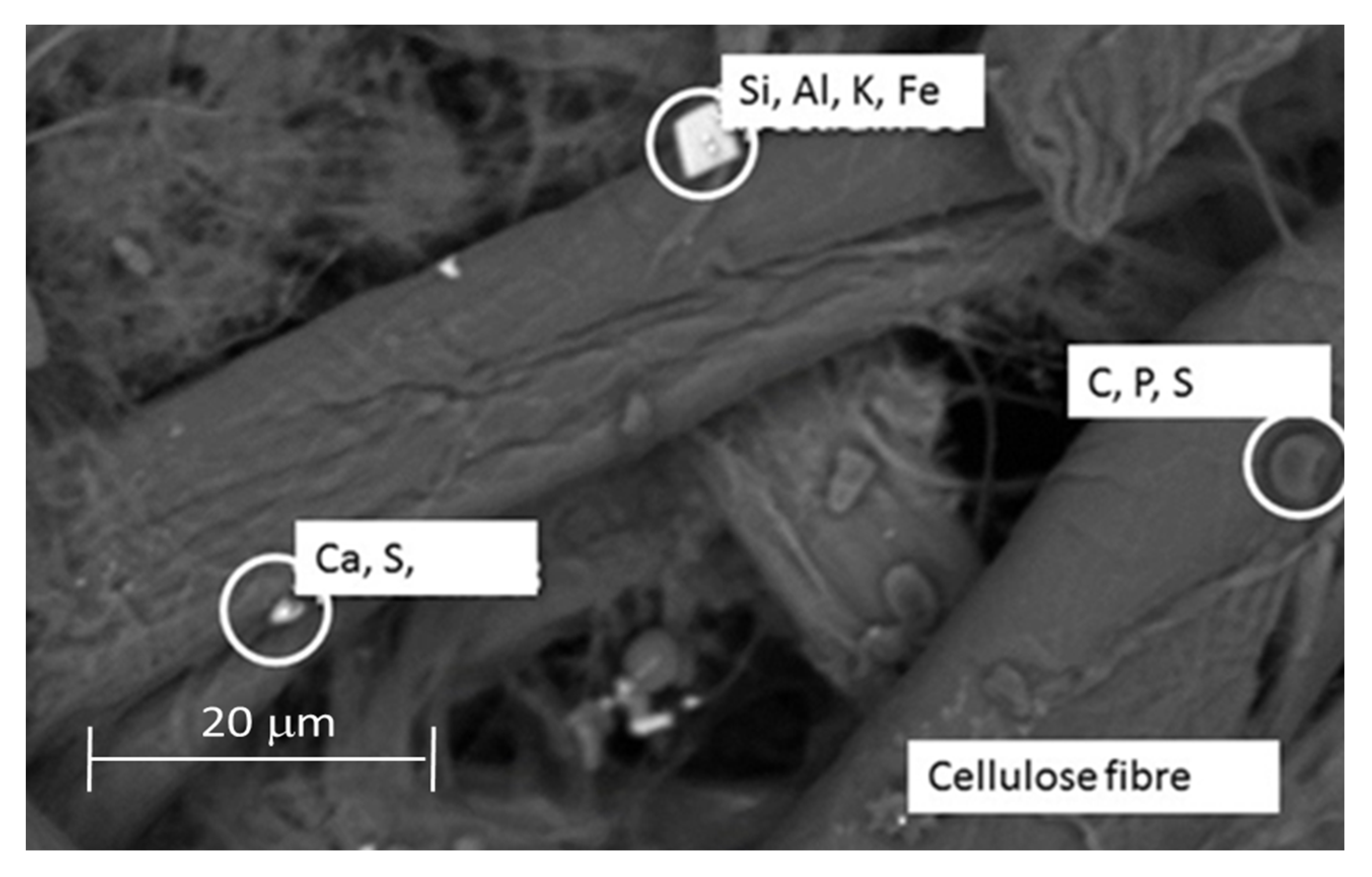
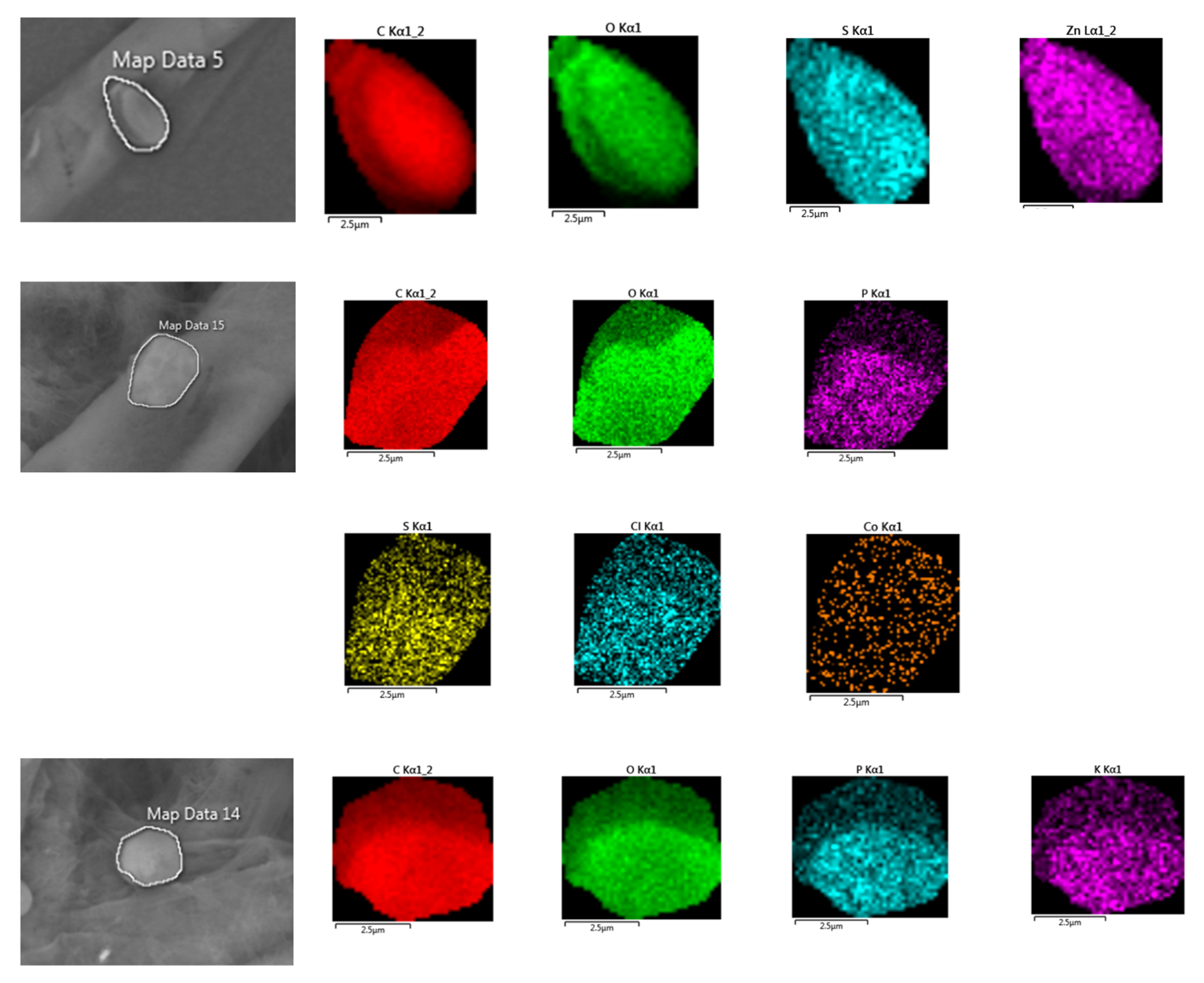
2.9. Scanning Electron Microscopy

All measurements were performed using the Hitachi SU-70 analytical field emission Scanning Electron Microscope (SEM) at the Central Science Laboratory, University of Tasmania. An area of approximately 1 cm2 of sample on Whatman 41 filter was covered by powdered carbon and analysed using an electron beam voltage of 15 kV. To find the best observation area, secondary electron (SE) images of the filter were collected [79]. Backscattered electrons (BSE) were used to determine average molecular masses of aerosols [79]. X-ray Energy Dispersive Spectrum (EDS) was applied to determine the elemental composition of the selected particles [79]. Two types of EDS measurements were applied: (1) in point measurements, where the electron beam hits a single point (within the particle surface) of a particle and (2) mapping of part of the filter or selected particle by the electron beam. Five samples were chosen for analysis (MB5, MB6, MB10, MB11, MB18A) based on predominant aerosol sources determined by leaching results, back trajectories, and wind patterns.

2.10. Enrichment Factor

The enrichment factor (EF) expresses the enrichment of a particular element in the particle relative to the global crust concentration. EF compares the ratio of the element (Z) with a mineral dust tracer (here Ti) in aerosols to the average content in the upper crustal layer [80] (3). Low values approaching 1 indicate that mineral dust is the main source of the element of interest in the atmosphere. A higher EF represents a higher contribution of non-crustal source. Elements were divided into three groups based on their median EF into (1) low, EF<2, (2) moderate, 2≤ EF<10, and (3) high, EF ≥10. This classification is similar to the one applied by Winton et al. [28] and Buck at al. [81] for an aerosol samples origin investigation.
EF = ([Z]/[Ti])atm./([Z]/[Ti]crust)
where [Z](atm.) indicates concentration of element Z in the atmosphere or in the average global crust [Z](crust).

2.11. Other Calculations

Fractional solubilities of Fe and other TMs are the relative contribution (in percent) of the atmospheric concentrations of (i) one fraction (soluble, leachable, or labile) to the atmospheric concentration to (ii) the total concentration of this element, which is the sum of soluble, leachable, and refractory fractions. FFeS was calculated by dividing the atmospheric concentration of soluble, leachable, and labile Fe by atmospheric concentration of total Fe (4).
e.g., %Fesoluble = 100% × [Fesoluble]atm./([Fesoluble]atm. + [Feleachable]atm. + [Ferefractory]atm.)
For studying FFeS correlations with anthropogenic emissions and combustion/biomass burning particulates, a Pearson correlation was applied. The Pearson correlation coefficient ‘r’ was compared with critical Pearson rc (p = 0.05 two tailed) for the specific number of pairs (n) expressed as a degree of freedom (df) where df = n − 2, to test the correlation significance (if rrc then the correlation is significant). The following correlation coefficient (r) denomination was applied: 0.00–0.19 very weak, 0.20–0.39 weak, 0.40–0.59 moderate, 0.60–0.79 strong, and 0.80–1.0 very strong [82].
The Fe dry deposition flux (Fdry) was calculated by multiplying the Fe concentration in air [Fe] atm. by the velocity of dry deposition (vdry) (5). Where [Fe]atm. is atmospheric Fe concentration and vdry is a dry deposition velocity.
Fdry = [Fe]atm. × vdry

3. Results and Discussion

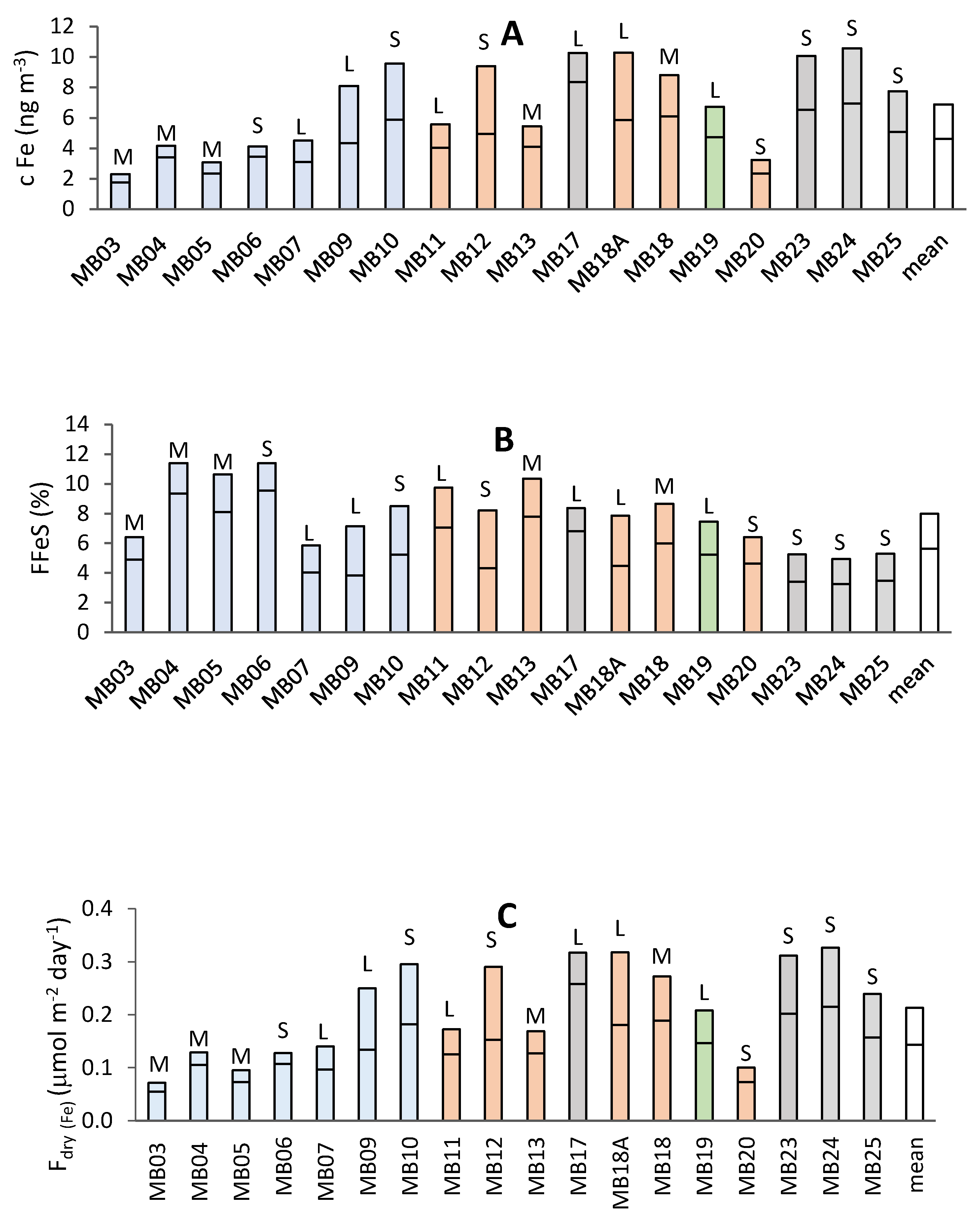
3.1. Iron in Aerosols

3.1.1. Iron Provenance

Enrichment factor of iron ranged from 0.6 to 1.2 (one outlier of 6.8 for sample MB6) with a median (± SD) of 0.9 ± 0.2, which indicates that most Fe originates from crustal materials. In addition, total Fe was very strongly correlated with the mineral dust tracers Al (r = 0.990) and Ti (r = 0.943).
Backscattered electron imaging (Figure 3) distinguished between two classes of particles, which included irregularly-shaped mineral dust and regularly-shaped carbonaceous particles. Among analyzed samples, almost all particulates containing Fe were alumino-silicates, which explains the high correlation between total Fe and Al. On the other hand, very few Fe oxide particulates were detected.
SEM observations suggest that alumino-silicates are the main source of total Fe. Iron from alumino-silicate lattices is generally more bioaccesible than from oxides due to greater chemical weathering rates [83], which may partially explain the relatively high FFeS observed in this study as discussed below.

3.1.2. Iron Solubility

The contribution of contamination from filter handling in the field increased the amount of Fe in the blank sample by 14.3%, 5.7%, and 4.9% for soluble, leachable, and refractory fraction, respectively, while the average contribution of Fe from the blank in the sample was 1.54 ± 0.53%, 6.37 ± 3.78%, and 4.03 ± 2.10% for soluble, leachable, and refractory fractions, respectively. Precision of the applied leaching protocol was determined based on triplicate analysis and was reported as 1.9%, 8.5%, and 9.5% for soluble, leachable, refractory fraction, respectively [3]. More details about the initial method assessment is provided in Appendix A. Based on determined atmospheric concentrations of soluble, leachable, and refractory Fe fractions, we calculated FFeS and dry deposition fluxes (Figure 4 and Table S3). Labile Fe concentrations ranged from 2.3 to 10.6 (mean ± SD 6.9 ± 2.9) ng m−3 while total Fe concentrations ranged from 29.0 to 213.7 (mean ± SD 95.2 ± 53.9) ng m−3. Atmospheric concentration of total Fe lies in the lower range of global model estimates forecast for this part of Australia, which are 40–1000 ng m−3 [84]. The labile Fe was 4.9%–11.4% (mean ± SD 8.0 ± 2.1%) of the total Fe content, and is at a similar level to the Fe solubility estimates from the global model, which forecasts an FFeS of 4%–10% for this part of Australia [85]. Between 52.6% and 83.7% (mean ± SD 69.4 ± 9.2%) of the labile Fe originated from the soluble (UPW) leach while the buffer leach provided an additional 16.3%–47.4% (mean ± SD 30.6 ± 9.2%). The fraction of labile Fe is inversely proportional to the total Fe content, which may be explained by the coexistence of two Fe pools characterized by (a) low and (b) high labile Fe content. The relative proportion of these factors drives the solubility of the mixture.
Reported values for Fe solubilities around Australia are sparse and variable between sampling sites. In this scenario, we are comparing data from the Misison Beach with results of FFeS of Australian aerosols and soils to get comparision in terms of ocean fetrilisation potential and sources. The FFeS results reported in this section are similar to data reported by Winton et al. [28] for aerosols collected at a coastal site in the Northern Territory (Australia) (2%–12%) and lie in the lower range of solubilities observed in Tasmania (0.5%–56%) [29]. The labile fraction of Fe in aerosols collected at Mission Beach is similar to those reported in aerosols collected at sea during the same period (4%–33%) [68]. Our results are higher than those reported by Mackie et al. [57] for readily soluble Fe (dissolving in the time range from minutes to hours) from soil samples collected in Thargomindah in Southwest Queensland (0.9 ± 0.3%). However, our findings are similar for dust samples collected in Burunga in the Mellee region between Victoria and New South Wales (5.6 ± 0.7%) [57]. Results presented in this study are also higher than previous findings for mineral dust from other regions, e.g., the fractrional Fe solubility was below 1% for Saharan dust [34,45] and 4.0 ± 0.5% for Chinese Loess [34]. FFeS also ranged from 0.02% to 0.4% for coarse dust from desert regions (Sahara, Arab Desert, and Thar Desert) collected in the Arabian Sea, while, for aerosols collected on the Bay of Bengal FFeS, it was much higher at 1.4%–24% [86]. Srinivas et al. [86] also reported a correlation between FFeS and non-sea salt sulfate (nss-SO42−), which suggests emissions from biomass burning and/or fossil fuel combustion was also present in samples from the Bay of Bengal. The higher FFeS of particles may be explained by a higher content of combustion particles from biomass burning and anthropogenic emission, which are more soluble than mineral dust.

3.1.3. Drivers of Iron Solubility

Non-Crustal Emissions vs. Iron Solubility

The correlations between soluble and leachable Fe fractions with total fractions of mineral dust tracers were much weaker than between total fractions of Fe and a mineral dust tracer. This indicated the existence of other sources of soluble Fe in aerosol samples. Thus, anthropogenic and crustal emissions were tested as a potential source of soluble and leachable Fe by analyzing correlation coefficients between them (Table 1). The correlations between FFeS with total fractions of non-crustal elements were also calculated. To consider mineral dust loadings for each sample, total atmospheric concentrations of an anthropogenic element (AE) was divided by the total atmospheric concentration of Ti. In general, significant correlations, between fractional FFeS and Ti normalised anthropogenic elements, were only observed for the soluble Fe fraction, but not the leachable fraction. Therefore, we focused only on the observed moderate (0.40 < r < 0.59) correlations between soluble Fe and Cd, Co, Cu, and Mn, and strong (0.60 < r < 0.79) correlations between soluble Fe with total Mo, Pb, V, and Zn normalized to Ti (Table 1).
To assign the non-crustal emissions to more specific sources, samples were divided into groups based on their marine and terrestrial origin, as identified by BT analysis (Figure S1) and (see 0 for more information about BT analysis). This provided information about sources and areas of possible mixing along the transport path. Local wind direction patterns (Figure 2) (sea breeze and land breeze) were also noted to assess the contribution from local anthropogenic emissions (0 for details about wind direction classification). A significant and strong (0.80 < r < 1) correlation was found between soluble Fe with Cd (r = 0.964), V (r = 0.892), and Zn (r = 0.786) for sea breeze samples. This may be explained by anthropogenic emissions from ships in the GBR region and/or from emission along the northern Queensland coast (transport, power plants, and fuel combustion) due to air masses usually passing along the coastline just prior to sampling. Moderate (Cd, Co, Mn) and even strong (Cu, Mo, Pb, V, Zn) correlations were observed for marine samples, but these results were not significant due to a limited number of samples for which the critical value of the Pearson coefficient was high. Studies of land-derived samples indicated a significant correlation between soluble Fe and Mn (r = 0.878) and V (r = 0.833) within the terrestrial group, and between soluble Fe and Pb (r = 0.833) within the land breeze group. For V, we also observed strong but not significant correlations for the land breeze group. Similarly, strong but not significant (due to a limited number of samples) correlation for both terrestrial and land breeze samples were observed for Cd and Co. Non-crustal emissions were an important source of soluble Fe, particularly for sea breeze air masses. Terrestrial-based anthropogenic emissions indicated that soluble Fe coexists in the air with Mn and V, according to BT origin classification, and with Pb, according to wind direction origin classification. Sedwick et al. [45] reported higher FFeS for aerosols collected in Bermuda when air masses passed over North America compared to those that passed over the Sahara. North American air masses were characterized by low total Fe content accompanied by elevated values of V/Al, Fe/Al, and V/Mn indicating anthropogenic combustion products. On the other hand, Fu et al. [46] found high correlation coefficients between FFeS and K from biomass burning and the V/Fe ratio in spring in Shanghai, which suggests that both biomass burning and oil ash from ship emissions are responsible for an increase in FFeS. Correlations between FFeS with V and Pb were observed in our study, which confirms anthropogenic origin of labile Fe.

Combustion Products vs. Iron Solubility

Black carbon (BC) is a proxy for combustion processes including fossil fuel and biomass burning. A correlation between the ratio of atmospheric concentrations of BC to total Fe with fractions of soluble, leachable, and labile Fe was investigated. This was analogous to the procedure applied by Fu et al. [46] in which K+ normalized to total Fe was used as biomass burning tracer and correlated with FFeS.
The soluble Fe was strongly positively correlated (r = 0.601, df= 15, p < 0.05) with BC/Fetotal, which indicates that the FFeS increases with increased concentrations of BC. In addition, a very strong (r = 0.851, df = 4, p < 0.05) correlation was observed between soluble Fe with BC/Fetotal within the group of sea breeze samples. Within this group, strong correlations between the percent of soluble Fe with Cd, V, and Zn were reported (Table 1). We, therefore, conclude that anthropogenic combustion processes, such as fossil fuel combustion, may provide soluble forms of Fe. No significant (p < 0.05) correlations were found for samples from other origins.
A moderate correlation (r = 0.50) was found between the percent of soluble Fe and both LG indicators (m/z 60 and 73). However, for this limited set of analyzed aerosol samples for which the LG data are available (df = 9), correlations were not significant. A significant (p < 0.05) correlation was observed only for sea breeze samples for which we calculated r = 0.95 and r = 0.92 (df = 3) for organics m/z = 60 and 73, respectively. This may indicate that FFeS originated from biomass burning emission from the land, and then transported above the sea before returning to the coast and/or from emissions from sources along the coast (e.g., sugar mills, which are also a source of LG). Within the sea breeze group, significant correlation was also found between soluble Fe and BC and Cd, V, and Zn. It has been reported that substantial proportion of anthropogenic elements, such as emissions from open mining, may be accumulated on the vegetation [87,88] and, consequently, then could be re-entrained to the atmosphere during the fire event.
The correlation between soluble Fe and both BC/Fetotal and LG/Fetotal in the atmosphere was observed in this study and agrees with previous reports [34,46,53] where combustion processes and biomass burning were found to provide a significant amount of soluble Fe. Therefore, we suggest that both sources enhance FFeS near the GBR. The Northern Queensland coast is both more densely populated compared to the inland and is a popular tourist destination with intensive ship movements across the GBRMoreover, this is an agricultural area with numerous sugar cane plantations and sugar mills, which produce energy by burning the bagasse, to generate electricity and steam for factory operations, while producing around 500 GWh [89]. Some of the sugar mills are in the proximity to the sampling site, in Tully (approx. 20 km S-E), South Johnstone (approximately 30 km N-E) and Mourilyan (approximately 35 km N-E) (National Pollution Inventory) (Figure 1). Similar to the enrichment of anthropogenic elements, we observed a higher correlation between the percentage of soluble Fe and total Fe normalized BC and LG during sea breeze conditions that may be explained by emissions from along the coast, from ship movements across the GBR, and emissions from the sugar mills located in close proximity to the sampling station. Bushfires occurring several hundred kilometers north-west and south-west of the sampling site around the time of sampling are another potential source of biomass burning emission [90]. However, due to limited LG data, this cannot be confirmed.
Observation of our samples by SEM confirm carbonaceous particulates were more abundant in some samples, particularly in these for which a high level of BC and LG was observed. Round shape particulates were more homogenously distributed across the filter area and their size range was more uniform compared to the minerals. These particles were 1–5 μm in size, which mainly consist of homogenously distributed C, P, and S. Some of the carbonaceous particles also contained homogenously distributed Zn, K, and Ca (Figure 5). These particles may be classified as tar balls, which is a common particle from natural and industrial biomass burning [91,92].

Aging Processes vs. Iron Solubility

Possible aging processes were studied by analyzing soluble major ion (MI) contents in our aerosol samples and correlating them with FFeS. Results indicate that relationships exist between the presence of aging agents represented by anions (e.g., NO3, nss-SO42−) and increased FFeS. Normalization of the MI atmospheric concentration to the total Fe atmospheric concentration was applied to minimize mineral dust contribution to MI content by following Fu et al. [46]. Strong and significant (p < 0.05) correlations between soluble Fe and total Fe normalized concentrations of NO3 (r = 0.669, df = 16) and nss-SO42− (r = 0.724, df = 16) were found, which indicates that aging processes may increase Fe solubility. For marine samples, the correlation for these anions was even stronger (and significant, p < 0.05): r = 0.767 for both (df = 5). A strong and significant (p < 0.05) correlation (r = 0.925, df = 4) was also found between nss-SO42− Fetotal−1 and FFeS for sea breeze samples (collected 6 AM–6 PM). There were no significant correlations for either land breeze samples (collected 6 PM–6 AM) or terrestrial samples. Our results indicate that NO3 and nss-SO42− anions coexist with soluble Fe. Both anions may exist in the atmosphere as acids or salts (commonly known as ammonium sulfate). Both nitric and sulphuric acids are derived from oxidation of precursor gases. Sulphur dioxide (SO2) originates from combustion processes or oxidation of dimethyl sulphide (produced by surface ocean biota) [93]. Nitrogen oxides (NOx) are produced from fossil fuel combustion and biomass burning [94], but also from lightening [95], soil emissions [96], and organic marine nitrate [97]. Nitric and sulphuric acid play two different roles: (1) as indicators of combustion processes, which provide highly soluble Fe and/or (2) as a source of protons, which increases FFeS for insoluble or low solubility Fe species such as minerals [98]. In this study, the correlation between FFeS and major ions indicates possible aging processes. However, correlations were also observed between FFeS and combustion and biomass burning emissions as well as elements of elevated EF. These observations suggest that major ions may simply be emitted together with the pyrogenic Fe.

3.1.4. Estimation of Fe Deposition Fluxes

Correlation coefficient between atmospheric concentrations of total Fe and total Ti was very high and their (atmospheric concentrations of total Fe and total Ti) ratio was similar to the value for the global average of the upper crust (see part 3.1.1. for details), which indicates a crustal origin that usually exists in the form of coarse particulates above 2.5 μm in size, and was confirmed by SEM images. A value of dry deposition velocity (Vdry) (4) is sensitive to the wind speed and humidity as well as particle size profile. For coarse crustal particulates, Vdry has been estimated to range from 0.3 to 3.0 cm s−1 [66] and was assumed of 2 cm s−1 for coastal regions of Australia [28,67,68] with uncertainty of 50% [28,29]. The calculated dry deposition Fe flux ranged from 0.055 ± 0.027 to 0.258 ± 0.129 μmol m−2 day−1 (mean 0.143 ± 0.072) for the soluble, 0.017 ± 0.008 to 0.138 ± 0.069 μmol m−2 day−1 (mean 0.070 ± 0.035) for the leachable, and 0.802 ± 0.401 to 6.27 ± 3.14 μmol m−2 day−1 (mean 2.73 ± 1.37) for the refractory Fe fraction. Hence, the total Fe deposition ranged from 0.897 ± 0.448 to 6.61 ± 3.31 μmol m−2 day−1 (mean 2.95 ± 1.47). However, soluble and labile Fe appeared to be linked with the anthropogenic emissions/combustion processes (see parts 3.1.3.1 and 3.1.3.2), which usually exist in fine mode (<2.5 m) and, consequently, their deposition flux may be lower (assumed as 0.2 cm s−1 in part 3.3 for anthropogenic elements). These finer particulates may reach more remote ocean areas.
The mean flux of labile Fe in this study was 0.213 ± 0.107 μmol m−2 day−1, which is lower than results of marine aerosols collected at sea (Coral Sea Marine Region) during the same time period, 0.303 ± 0.590 μmol m−2 day−1 [68] calculated based on the same deposition velocity. Fluxes reported in this case are also similar to the lower results reported by Winton et al. [28] for Northern Territory, 0.2 ± 0.1–4 ± 2 μmol m−2 day−1 (also calculated for the same deposition velocity). The Northern Territory samples were collected during the dry season and had more land than marine-based origin compared to the samples collected in this study.

3.2. Iron in Rain Water

The fluxes of Fe provided by two rain events combined were 0.165, 0.195, and 0.659 μmol m−2, for soluble, total-dissolvable, and particulate fractions, respectively. This corresponded to 16.2%, 19.2%, and 64.6% of total Fe in the rain, respectively. The second rain event provided more Fe (soluble as well as suspended and refractory) despite providing approximately five times less rainfall. Rain events tend to wash out the particulates from the atmophere at the beginning of the rain event. In case of the first rain events in our study, the amount of washed out iron was likely highly diluted by the cleaner rain water falling in the later parts of the rain event. The wet deposition flux of soluble Fe exceeded the dry deposition soluble Fe flux recorded on this day (0.073 μmol m−2 day−1) as well as the average dry deposition for the entire sample set (0.143 μmol m−2 day−1). Consequently, the amount of soluble Fe deposited in two rain events is equal to soluble Fe depostited by dry deposition for 28 h if the average for the sampling campaign soluble Fe flux is applied. These results highlight the importance of wet deposition as a source of soluble Fe during the dry season in Northern Queensland. It is worth noting the difference in Fe concentrations in two rain events occurring on the same day. Variability may be much greater when considering rain events occurring in different parts of the year and depending on BT of air masses. These wet deposition Fe results gives 0.248 μmol m−2 of soluble Fe flux in wet deposition in total during the sampling period. The average fraction of soluble Fe in collected rain water samples was 16.2%, which is twice as high as FFeS for dry deposition samples collected on the same day of the rain event (8.1% for soluble and 10.6% for labile). Similar FFeS for dry and wet depositions was also reported for most of the rain samples collected over the Sargasso Sea (typically below 4%) [45] and the Mediterranean Sea (0.5%–27%) [99]. Theodosi et al. [99] also identified strong source and acidity influences on this parameter. Leaching experiments conducted on samples from the same region revealed FFeS of approximately 1% and 12% for Saharan dust and anthropogenic emission, respectively [100]. Our study confirmed the significant role of single wet deposition events as a source of soluble Fe, as previously reported [67,101]. Moreover, long-term records indicate that rainfall is typically higher than observed during our campaign, which suggests that the contribution of wet Fe deposition to the total Fe deposition may be even higher.

3.3. Atmospheric Deposition of Coral Toxins and Other Bioactive Metals

Origins of Cd, Co, Cu, Mn, Mo, Pb, V, and Zn were investigated based on the EF analysis, by following the method described in 2.10 using Equation (3). Due to concentrations spanning several orders of magnitude, log(EF) is presented on a linear scale (Figure 6). Elements were divided into three groups based on their median EF into (1) low, EF <2: Co, Fe, Mn, (2) moderate, 2≤ EF <10: Mo, Pb, V, and (3) high, EF ≥10: Cd, Cu, Zn. Results indicate a significant contribution of non-mineral dust sources to the atmospheric TMs content at Mission Beach. Only Co and Mn (in addition to Fe) had a low EFs indicating mostly a crustal origin. Moderate contributions of anthropogenic emissions were observed for Mo, Pb, and V, which were classified as having a mixed origin overall. Lastly, Cd, Cu, and Zn had the highest EFs and, thus, we assumed they were mostly emitted by anthropogenic sources. However, Shotyk et al. [102] reported the relatively elevated EF for ancient peat samples originating from the mid-Holoscene and Boutron et al. [103] found severe variations and peaks of Cd in the Antarctic ice and snow in the last 155,000 years, which may not be simply accounted for by crustal emissions and volcano eruptions. Correlation of analysed TMs with the mineral dust tracers, Al and Ti, was weaker for elements of higher EF and the correlation increases with the drop of EF between elements, which confirms that Fe, Co, and Mn had a crustal origin while Cd, Cu, Zn, Mo, V, and Pb were rather independent on the mineral dust concentration (Figure 6).
The main delivery of heavy metals to the GBR has been linked with riverine discharges associated with agriculture and stormwater runoff, and waste water from ships [104]. In this case, we studied atmospheric deposition as an additional source of heavy metals to GBR. Atmospheric concentrations of total and labile forms of elements, which were found to have toxic influences on corals, Cu, Zn, and Cd [21,23,24,25], were determined. Deposition fluxes of labile fractions were estimated to assess the amount that may be available to marine biota (Table S4). The calculations were analogous to these for Fe (details in 3.1.2), but an order of magnitude lower deposition velocity (0.2 cm s−1) was applied for Cd, Cu, Mo, Pb, V, and Zn since they showed mixed or anthropogenic signatures, which typically exists in the finer form than mineral dust [66]. The mean (±SD) atmospheric concentration of total Cu was 1.54 ± 1.62 ng m−3 while the fraction of labile Cu was 52.6 ± 23.2%, which results in a flux of labile Cu of 1.74 ± 0.87 nmol m−2 day−1. The mean ( ± SD) atmospheric concentration of total Cd was 0.069 ± 0.11 ng m−3 with 96.7 ± 4.0% in the labile form, which results in a flux of 0.11 ± 0.05 nmol m−2 day−1 of labile Cd. Analogous values for Zn were 3.50 ± 2.15 ng m−3, 84.6 ± 19.5%, and 7.93 ± 3.95 nmol m−2 day−1. All of these elements (Cd, Cu, and Zn) showed an anthropogenic signature and relatively high fraction of the labile form.
Deposition fluxes of potentially bioavailable forms of TMs obtained in this study were compared to the estimations for the riverine freshwater delivery based on data of discharged water volume to the GBR from Fabricius et al. [105] and TM concentrations measured in the Port Curtis estuary (Queensland) [71] (Table 2). We acknowledge the large uncertainty of this comparison as a result of (1) using short term data on atmospheric deposition (18 aerosol samples and 2 rain samples) not reflecting the seasonal variations, (2) using data from one sampling point for atmospheric deposition and two catchements for riverine input, which do not represent the diversity of the large area of GBR and its catchment, and (3) uncertainties of the calculation of deposition fluxes and riverine imputs. However, the aim of this comparison was to test the hypothesis that atmospheric deposition of heavy metals may be comparable to riverine discharge, which is currently considered to be the largest source of nutrients and contaminants.
Atmospheric deposition provides more Zn in both dry (7.9 ± 1.4 μmol m−2 y−1) and wet (40.1 ± 5.9 μmol m−2 y−1) form when compared to riverine input (5.5 ± 2.5 μmol m−2 y−1). Wet deposition is also an important carrier of soluble Cd (1.26 ± 0.54 μmol m−2 y−1), ahead of riverine input (0.19 ± 0.17 μmol m−2 y−1) and dry deposition (0.04 ± 0.06 μmol m−2 y−1). On the other hand, rivers deliver the majority of dissolved Cu (22.0 ± 4.9 μmol m−2 y−1) more than wet (8.0 ± 0.7μmol m−2 y−1) and dry (0.6 ± 0.4 μmol m−2 y−1) deposition. Therefore, atmospheric deposition cannot be neglected as a source of toxins [21] as it may be delivered to remote sites of the GBR in a more effective way than freshwater discharges. Heavy metals have been previously shown to cause a reduction of spawning efficiency [23,24,106] and a strong accumulation of toxins by corals [107,108]. In addition, coral spawning occurs for a few nights in late spring or early summer before the wet season. This suggests that, at the time of spawning, riverine delivery of toxins is limited and, consequently, the atmospheric deposition contribution may be even greater. Iron fluxes could not be compared due to the lack of riverine Fe data. Further investigations are needed to understand the significance of atmospheric deposition of toxins to the GBR.

4. Conclusions

The application of leaching experiments followed by bulk analysis of trace metals in aerosol samples resulted in a unique data set of atmospheric TM deposition to a globally significant coral region known as the Great Barrier Reef. Our study showed that mineral dust, particularly alumina-silicates, was the main source of total Fe. However, Fe from mineral dust was not a dominant source of soluble and labile forms of Fe. We observed relatively high Fe solubility near the GBR, which was linked to Fe originating from anthropogenic emissions such as fossil fuel combustion and biomass burning. Furthermore, we revealed that a prevalent proportion of coral toxins such as Cu, Zn, or Pb delivered from the atmosphere originate from combustion processes including anthropogenic emissions. Due to their high solubility, they may enter the local food chains rapidly. Combustion processes are currently growing due to climate change (more frequent bushfires in Australia) and growing industrial and touristic development of Queensland (higher emission of anthropogenic aerosols). Therefore, ocean fertilization of the GBR by labile Fe may be expected to increase in the future. The previously mentioned processes are also a source of potential toxins, and our study indicates their contribution should not be neglected in the total toxic element delivery budget. Evaluation of effects of the atmospheric TM deposition on the GBR ecosystem was beyond the aim of this study. However, our study emphasizes the importance of atmospheric deposition of TMs in the GBR region including Fe and toxic elements. Our study is limited to land-based investigations in a rural part of Australia. Further work is required to understand the effect of natural and anthropogenic atmospheric TM emissions on coral reefs. Lastly, our results of Fe deposition fluxes reported here match the global Fe atmospheric deposition models in terms of atmospheric concentration of total Fe and FFeS [84], despite the fact that there is limited data for the models for the Southern Hemisphere. Our study also raises the importance of wet deposition, which may deliver a great quantity of TMs in a short time frame.

Supplementary Materials

The following are available online at https://www.mdpi.com/2073-4433/11/4/390/s1: Figure S1. Air mass back trajectories of the aerosol samples and consequent origin classification, Table S1. Dry deposition aerosol samples log sheet. Measured volume was corrected to the temperature and pressure conditions, Table S2. Classification of aerosol samples based on their origin. Table S3. Fractional solubility, atmospheric concentration, and dry deposition flux of Fe, Table S4. Mean (±SD) values of total atmospheric concentration, labile fraction, and dry deposition flux of bioactive elements.

Author Contributions

Project conception (A.R.B.), data interpretation (M.S., B.C.P., A.R.B., M.G.-R.), writing manuscript (M.S.), reviewing manuscript (all authors), designing experiments (M.S., A.R.B., B.C.P., M.G.-R., P.W.B., M.M.G.P.), aerosol sample collection (M.S., R.G.R.), laboratory work (M.S., M.M.G.P., M.G.-R.), AMS data (Z.D.R., J.A.), MAAP data (R.S.H., M.D.K. and J.W.), wind data (R.S., R.G.R.), and fieldwork commanding (R.S., Z.D.R.). All authors have read and agreed to the published version of the manuscript.

Funding

This work was supported by an Australian Research Council Future Fellowship to A.R.B. (FT130100037), an ARC Linkage, Infrastructure, Equipment and Facilities (LE150100048), the Antarctic Climate & Ecosystems Cooperative Research Centre, an ARC Discovery Project (DP150101649) to Z.D.R. and the ARC Centre of Excellence for Climate System Science (CE110001028) grants to R.S.

Acknowledgments

Chemical analysis of ICP-MS and SEM were conducted at the CSL while IC at ACROSS and Ashley Townsend (ICP-MS), Karsten Goemann (SEM), and Brett Paul (IC) are gratefully acknowledged. The authors gratefully acknowledge Thomas Holmes and Luis Duprat for their help in reading earlier versions of this manuscript. The authors gratefully acknowledge the NOAA Air Resources Laboratory (ARL) for the provision of the HYSPLIT transport and dispersion model and/or READY website (http://www.ready.noaa.gov) used in this publication.

Conflicts of Interest

The authors declare no conflict of interest.

Appendix A. Analytical Methods Check

Appendix A.1. Iron Blanks

Two types of blank samples were analyzed to track sources of contamination during filter handling in the field when TM clean conditions were unavailable, and a simple house-made ‘clean-box’ (Figure A1) was used to minimize contamination issues. The laboratory blank (LB) is a clean filter, which has not been used for aerosol collection (remaining double bagged until processing) while the procedural blank (PB) is a filter exposed on the sampler for 10 min with the vacuum pump being turned off. Results presented below are for a 47-mm diameter filter punches of both LB and PB filters. More details are available from Perron et al. [3].
Figure A1. Cassette with filter inside ‘the clean-box’ during routine filter changeover.
Atmosphere 11 00390 g0a1
The averaged values of four LB and three PB samples were 1.8 ng and 2.1 ng per filter, respectively, for the soluble Fe fraction, and 3.3 ng and 3.5 ng per filter for the leachable Fe fraction and 87.1 and 91.6 ng for the refractory Fe fraction. The difference between these two blanks (LB and PB) can be used as an indicator of contamination caused by handling of the filter. Consequently, the Fe content in PB was 14.3%, 5.7%, and 4.9% higher than in LB for soluble, leachable, and refractory fractions, respectively. Increase (between LB and PB) in the soluble fraction of Fe is considerate. However, the blank contribution in relation to the amount of soluble Fe contained in aerosol samples was, in most cases, below 2% (blue dots in Figure A2). This proves that applied in-field laboratory conditions and leaching protocol did not cause serious sample contamination and, consequently, they were suitable for TM clean handling of filters in the field.
The average PB has been used to correct sample concentration because this blank accounts for every stage of possible contamination. The single standard deviation from blank replicates has been used for uncertainty calculation. Generally, the average contribution of the PB to the Fe content in samples was 1.54 ± 0.53%, 6.37 ± 3.78%, and 4.03 ± 2.10 for soluble, leachable, and refractory fractions, respectively. Data for individual samples are given in Figure A2.
Figure A2. Contribution of procedural blanks to the Fe content in the samples for soluble (blue), leachable (green), and refractory (orange) fractions. Error bars calculated based on single standard deviations between separated PB’s collected in Mission Beach.
Atmosphere 11 00390 g0a2

Appendix A.2. Digestion Procedure Recovery

Recovery of the digestion procedure was measured for the reference materials, which aim to mimic the mineral dust. Arizona Test Dust and Köln Loess GeoPT13 were digested and analysed in the same way as the filter sub-samples. Recoveries using the digestion procedure presented in this case were a subject of analytical method development and was already reported by Perron et al. [3]. Reported recovery for Fe was 102% and 104% for Arizona Test Dust and Köln Loess, respectively [3]. The recoveries were 99% and 105% for Al, 97% and 103% for Co, 102% and 109% for Cu, 99% and 105% for Mn, 82% and 80% for Pb, 100% and 84% for Ti, and 94% and 100% for V [3].

Appendix A.3. Precision of the Leaching Protocol and Digestion

To test the sample’s homogeneity (aerosol distribution across the filter) and precision of the applied leaching protocol, triplicate analysis of one sample has been conducted. Data from triplicate analysis was used to determine relative standard deviation and was 1.9%, 8.4%, and 9.5% for soluble, leachable, and refractory fraction of Fe, which gives 9.5% of uncertainty in total Fe fractions [3].

References

  1. Jickells, T.; Moore, C.M. The Importance of Atmospheric Deposition for Ocean Productivity. Annu. Rev. Ecol. Evol. Syst. 2015, 46, 481–501. [Google Scholar] [CrossRef]
  2. Jickells, T.D. Global Iron Connections Between Desert Dust, Ocean Biogeochemistry, and Climate. Science 2005, 308, 67–71. [Google Scholar] [CrossRef] [PubMed] [Green Version]
  3. Perron, M.M.G. Assessment of leaching protocols to determine the solubility of trace metals in aerosols. Talanta 2020, 208, 120377. [Google Scholar] [CrossRef] [PubMed]
  4. Morel, F.M.M.; Price, N. The Biogeochemical Cycles of Trace Metals in the Oceans. Science 2003, 300, 944–947. [Google Scholar] [CrossRef] [Green Version]
  5. Henderson, G. GEOTRACES—An international study of the global marine biogeochemical cycles of trace elements and their isotopes. Chemie Der Erde Geochem. 2007, 67, 85–131. [Google Scholar]
  6. Lohan, M.C.; Tagliabue, A. Oceanic Micronutrients: Trace Metals that are Essential for Marine Life. Elements 2018, 14, 385–390. [Google Scholar] [CrossRef]
  7. Lønborg, C. The Great Barrier Reef: A source of CO 2 to the atmosphere. Mar. Chem. 2019, 210, 24–33. [Google Scholar] [CrossRef]
  8. Morrison, T.; Hughes, T. Climate change and the Great Barrier Reef. Policy Information Brief 1; National Climate Change Adaptation Research Facility: Gold Coast, Australia, 2016. [Google Scholar]
  9. Brodie, J. Dispersal of suspended sediments and nutrients in the Great Barrier Reef lagoon during river-discharge events: Conclusions from satellite remote sensing and concurrent flood-plume sampling. Mar. Freshw. Res. 2010, 61, 651–664. [Google Scholar] [CrossRef]
  10. Brand, L.E. Minimum iron requirements of marine phytoplankton and the implications for the biogeochemical control of new production. Limnol. Oceanogr. 1991, 36, 1756–1771. [Google Scholar] [CrossRef]
  11. Kustka, A.B. Iron requirements for dinitrogen- and ammonium-supported growth in cultures of Trichodesmium (IMS 101): Comparison with nitrogen fixation rates and iron: Carbon ratios of field populations. Limnol. Oceanogr. 2003, 48, 1869–1884. [Google Scholar] [CrossRef] [Green Version]
  12. Cropp, R.A. The likelihood of observing dust-stimulated phytoplankton growth in waters proximal to the Australian continent. J. Mar. Syst. 2013, 117–118, 43–52. [Google Scholar] [CrossRef] [Green Version]
  13. Shaw, E.C.; Gabric, A.J.; McTainsh, G.H. Impacts of aeolian dust deposition on phytoplankton dynamics in Queensland coastal waters. Mar. Freshw. Res. 2008, 59, 951–962. [Google Scholar] [CrossRef]
  14. Shaw, E.C.; Gabric, A.J.; McTainsh, G.H. Response to comment on Impacts of aeolian dust deposition on phytoplankton dynamics in Queensland coastal waters. Mar. Freshw. Res. 2010, 61, 504–506. [Google Scholar] [CrossRef] [Green Version]
  15. Mackie, D.S. Biogeochemistry of iron in Australian dust: From eolian uplift to marine uptake. Geochem. Geophys. Geosyst. 2008, 9, Q03–Q08. [Google Scholar] [CrossRef]
  16. Boyd, P.W.; Mackie, D.S.; Hunter, K.A. Aerosol iron deposition to the surface ocean - Modes of iron supply and biological responses. Mar. Chem. 2010, 120, 128–143. [Google Scholar] [CrossRef]
  17. Falkowski, P.G. Evolution of the nitrogen cycle and its influence on the biological sequestration of CO2 in the ocean. Nature 1997, 387, 272–275. [Google Scholar] [CrossRef]
  18. Berman-Frank, I. Iron availability, cellular iron quotas, and nitrogen fixation in Trichodesmium. Limnol. Oceanogr. 2001, 46, 1249–1260. [Google Scholar] [CrossRef]
  19. Mills, M.M. Iron and phosphorus co-limit nitrogen fixation in the eastern tropical North Atlantic. Nature 2004, 429, 292–294. [Google Scholar] [CrossRef]
  20. LaRoche, J.; Breitbarth, E. Importance of the diazotrophs as a source of new nitrogen in the ocean. J. Sea Res. 2005, 53, 67–91. [Google Scholar] [CrossRef]
  21. Kroon, F.J. Sources, presence and potential effects of contaminants of emerging concern in the marine environments of the Great Barrier Reef and Torres Strait, Australia. Sci. Total Environ. 2020, 719, 135140. [Google Scholar] [CrossRef]
  22. Taylor, M.P. Atmospherically deposited trace metals from bulk mineral concentrate port operations. Sci. Total Environ. 2015, 515–516, 143–152. [Google Scholar] [CrossRef] [PubMed]
  23. Reichelt-Brushett, A.; Michalek-Wagner, K. Effects of copper on the fertilization success of the soft coral Lobophytum compactum. Aquat. Toxicol. 2005, 74, 280–284. [Google Scholar] [CrossRef] [PubMed]
  24. Reichelt-Brushett, A.J.; Harrison, P.L. The effect of copper, zinc and cadmium on fertilization success of gametes from scleractinian reef corals. Mar. Pollut. Bull. 1999, 38, 182–187. [Google Scholar] [CrossRef]
  25. Deschaseaux, E. High zinc exposure leads to reduced dimethylsulfoniopropionate (DMSP) levels in both the host and endosymbionts of the reef-building coral Acropora aspera. Mar. Pollut. Bull. 2018, 126, 93–100. [Google Scholar] [CrossRef] [PubMed]
  26. Mahowald, N.M. Observed 20th century desert dust variability: Impact on climate and biogeochemistry. Atmos. Chem. Phys. 2010, 10, 10875–10893. [Google Scholar] [CrossRef] [Green Version]
  27. Strzelec, M. Atmospheric Trace Metal Deposition from Natural and Anthropogenic Sources in Western Australia. Submited to Atmosphere in March 2020.
  28. Winton, V.H.L. Dry season aerosol iron solubility in tropical northern Australia. Atmos. Chem. Phys. Discuss. 2016, 16, 12829–12848. [Google Scholar] [CrossRef] [Green Version]
  29. Winton, V.H.L. Fractional iron solubility of atmospheric iron inputs to the Southern Ocean. Mar. Chem. 2015, 177, 20–32. [Google Scholar] [CrossRef]
  30. Journet, E. Mineralogy as a critical factor of dust iron solubility. Geophys. Res. Lett. 2008, 35, 12829–12848. [Google Scholar] [CrossRef] [Green Version]
  31. Ito, A. Pyrogenic iron: The missing link to high iron solubility in aerosols. Sci. Adv. 2019, 5, eaau7671. [Google Scholar] [CrossRef] [Green Version]
  32. Scanza, R.A. Atmospheric processing of iron in mineral and combustion aerosols: Development of an intermediate-complexity mechanism suitable for Earth system models. Atmos. Chem. Phys. 2018, 18, 14175–14196. [Google Scholar] [CrossRef] [Green Version]
  33. Desboeufs, K.V. Dissolution and solubility of trace metals from natural and anthropogenic aerosol particulate matter. Chemosphere 2005, 58, 195–203. [Google Scholar] [CrossRef] [PubMed]
  34. Schroth, A.W. Iron solubility driven by speciation in dust sources to the ocean. Nat. Geosci. 2009, 2, 337–340. [Google Scholar] [CrossRef]
  35. Huang, X.-F. Water-soluble organic carbon and oxalate in aerosols at a coastal urban site in China: Size distribution characteristics, sources, and formation mechanisms. J. Geophys. Res. Atmos. 2006, 111, D22212. [Google Scholar] [CrossRef]
  36. Matsuki, A. Morphological and chemical modification of mineral dust: Observational insight into the heterogeneous uptake of acidic gases. Geophys. Res. Lett. 2005, 32, L22806. [Google Scholar] [CrossRef] [Green Version]
  37. Zuo, Y.; Zhan, J. Effects of oxalate on Fe-catalyzed photooxidation of dissolved sulfur dioxide in atmospheric water. Atmos. Environ. 2005, 39, 27–37. [Google Scholar] [CrossRef]
  38. Cwiertny, D.M. Characterization and acid-mobilization study of iron-containing mineral dust source materials. J. Geophys. Res. Atmos. 2008, 113, D05202. [Google Scholar] [CrossRef]
  39. Fu, H. Photoreductive dissolution of Fe-containing mineral dust particles in acidic media. J. Geophys. Res. Atmos. 2010, 115, D11304. [Google Scholar] [CrossRef]
  40. Dupart, Y. Mineral dust photochemistry induces nucleation events in the presence of SO2. Proc. Natl. Acad. Sci. USA 2012, 109, 20842–20847. [Google Scholar] [CrossRef] [Green Version]
  41. Shi, Z. Formation of iron nanoparticles and increase in iron reactivity in mineral dust during simulated cloud processing. Environ. Sci. Technol. 2009, 43, 6592–6596. [Google Scholar] [CrossRef]
  42. Mackie, D.S. Simulating the cloud processing of iron in Australian dust: pH and dust concentration. Geophys. Res. Lett. 2005, 32, L06809. [Google Scholar] [CrossRef]
  43. Spokes, L.J.; Jickells, T.D. Factors controlling the solubility of aerosol trace metals in the atmosphere and on mixing into seawater. Aquat. Geochem. 1995, 1, 355–374. [Google Scholar] [CrossRef]
  44. Winton, V.H.L. Multiple sources of soluble atmospheric iron to Antarctic waters. Glob. Biogeochem. Cycles 2016, 30, 421–437. [Google Scholar] [CrossRef] [Green Version]
  45. Sedwick, P.N.; Sholkovitz, E.R.; Church, T.M. Impact of anthropogenic combustion emissions on the fractional solubility of aerosol iron: Evidence from the Sargasso Sea. Geochem. Geophys. Geosyst. 2007, 8, Q10Q06. [Google Scholar] [CrossRef]
  46. Fu, H.B. Fractional iron solubility of aerosol particles enhanced by biomass burning and ship emission in Shanghai, East China. Sci. Total Environ. 2014, 481, 377–391. [Google Scholar] [CrossRef] [PubMed]
  47. Shafizadeh, F. Production of levoglucosan and glucose from pyrolysis of cellulosic materials. J. Appl. Polym. Sci. 1979, 23, 3525–3539. [Google Scholar] [CrossRef]
  48. Simoneit, B.R.T. Levoglucosan, a tracer for cellulose in biomass burning and atmospheric particles. Atmos. Environ. 1999, 33, 173–182. [Google Scholar] [CrossRef]
  49. Rodriguez, E.S. Analysis of levoglucosan and its isomers in atmospheric samples by ion chromatography with electrospray lithium cationisation—Triple quadrupole tandem mass spectrometry. J. Chromatogr. A 2019, 1610, 460557. [Google Scholar] [CrossRef]
  50. Yu, X. Recyclable silver nanoplate-decorated copper membranes for solid-phase extraction coupled with surface-enhanced Raman scattering detection. Anal. Methods 2018, 10, 1353–1361. [Google Scholar] [CrossRef]
  51. Liang, L. Biomass burning impacts on ambient aerosol at a background site in East China: Insights from a yearlong study. Atmos. Res. 2020, 231, 104660. [Google Scholar] [CrossRef]
  52. Catelani, T.; Pratesi, G.; Zoppi, M. Raman Characterization of Ambient Airborne Soot and Associated Mineral Phases. Aerosol Sci. Technol. 2014, 48, 13–21. [Google Scholar] [CrossRef] [Green Version]
  53. Desboeufs, K.; Cautenet, G. Transport and mixing zone of desert dust and sulphate over Tropical Africa and the Atlantic Ocean region. Atmos. Chem. Phys. 2005, 5, 5615–5644. [Google Scholar] [CrossRef] [Green Version]
  54. Siefert, R.L.; Johansen, A.M.; Hoffmann, M.R. Chemical characterization of ambient aerosol collected during the southwest monsoon and intermonsoon seasons over the Arabian Sea: Labile-Fe(II) and other trace metals. J. Geophys. Res. Atmos. 1999, 104, 3511–3526. [Google Scholar] [CrossRef] [Green Version]
  55. Takahashi, Y. Seasonal changes in Fe species and soluble Fe concentration in the atmosphere in the Northwest Pacific region based on the analysis of aerosols collected in Tsukuba, Japan. Atmos. Chem. Phys. 2013, 13, 7695–7710. [Google Scholar] [CrossRef] [Green Version]
  56. Rudnick, R.; Gao, S. Composition of the Continental Crust. Treatise Geochem 3:1-64. Treatise Geochem. 2003, 3, 1–64. [Google Scholar]
  57. Mackie, D.S. Soil abrasion and eolian dust production: Implications for iron partitioning and solubility. Geochem. Geophys. Geosyst. 2006, 7, Q12Q03. [Google Scholar] [CrossRef]
  58. Vassilev, S.V. An overview of the composition and application of biomass ash. Part 1. Phase–mineral and chemical composition and classification. Fuel 2013, 105, 40–76. [Google Scholar] [CrossRef]
  59. Vassilev, S.V.; Vassileva, C.G.; Baxter, D. Trace element concentrations and associations in some biomass ashes. Fuel 2014, 129, 292–313. [Google Scholar] [CrossRef]
  60. Butler, A. Acquisition and Utilization of Transition Metal Ions by Marine Organisms. Science 1998, 281, 207–209. [Google Scholar] [CrossRef] [Green Version]
  61. Morel, F.M.M.; Milligan, A.J.; Saito, M.A. 6.05—Marine Bioinorganic Chemistry: The Role of Trace Metals in the Oceanic Cycles of Major Nutrients. In Treatise on Geochemistry; Holland, H.D., Turekian, K.K., Eds.; Pergamon: Oxford, UK, 2003. [Google Scholar]
  62. Fishwick, M.P. Impact of surface ocean conditions and aerosol provenance on the dissolution of aerosol manganese, cobalt, nickel and lead in seawater. Mar. Chem. 2018, 198, 28–43. [Google Scholar] [CrossRef]
  63. ARC Centre for Excellence for Climate System Science. Available online: https://www.climatescience.org.au/content/1130-reef-rainforest-campaign (accessed on 13 April 2020).
  64. AIRBOX, Reef to Reefforest. Available online: https://airbox.earthsci.unimelb.edu.au/reef-to-rainforest/ (accessed on 13 April 2020).
  65. AIRBOX A Mobile Air Chemistry Laboratory. Available online: https://airbox.earthsci.unimelb.edu.au/ (accessed on 13 April 2020).
  66. Duce, R.A. The atmospheric input of trace species to the world ocean. Glob. Biogeochem. Cycles 1991, 5, 193–259. [Google Scholar] [CrossRef]
  67. Baker, A.R. Dry and wet deposition of nutrients from the tropical Atlantic atmosphere: Links to primary productivity and nitrogen fixation. Deep Sea Res. Part I Oceanogr. Res. Pap. 2007, 54, 1704–1720. [Google Scholar] [CrossRef]
  68. Perron, M.M.G. Origin, transport and deposition of aerosol iron to Australian coastal waters. Atmos. Environ. 2020, 228, 117432. [Google Scholar] [CrossRef]
  69. Morton, P.L. Methods for the sampling and analysis of marine aerosols: Results from the 2008 GEOTRACES aerosol intercalibration experiment. Limnol. Oceanogr. Methods 2013, 11, 62–78. [Google Scholar] [CrossRef] [Green Version]
  70. Cutter, G. Sampling and Sample-Handling Protocols for GEOTRACES Cruises. Version 3. Available online: https://epic.awi.de/id/eprint/34484/ (accessed on 13 April 2020).
  71. Angel, B. Spatial variability of cadmium, copper, manganese, nickel and zinc in the Port Curtis Estuary, Queensland, Australia. Mar. Freshw. Res. 2010, 61, 170–183. [Google Scholar] [CrossRef] [Green Version]
  72. Stein, A.F. NOAA’s HYSPLIT Atmospheric Transport and Dispersion Modeling System. Bull. Am. Meteorol. Soc. 2015, 96, 2059–2077. [Google Scholar] [CrossRef]
  73. Rolph, G.; Stein, A.; Stunder, B. Real-time Environmental Applications and Display System: Ready. Environ. Model. Softw. 2017, 95, 210–228. [Google Scholar] [CrossRef]
  74. Bowie, A.R. Modern sampling and analytical methods for the determination of trace elements in marine particulate material using magnetic sector inductively coupled plasma–mass spectrometry. Anal. Chim. Acta 2010, 676, 15–27. [Google Scholar] [CrossRef]
  75. Keene, W.C. Sea-salt corrections and interpretation of constituent ratios in marine precipitation. J. Geophys. Res. Atmos. 1986, 91, 6647–6658. [Google Scholar] [CrossRef]
  76. Thermo Scientific Model 5012 MAAP Multi Angle Absorption Photometer. Available online: https://www.aires.com.br/wp-content/uploads/2018/01/5012-MAAP.pdf (accessed on 13 April 2020).
  77. Aerodyne Research, Aerosol Mass Spectrometer. Available online: http://www.aerodyne.com/products/aerosol-mass-spectrometer (accessed on 13 April 2020).
  78. Alfarra, M.R. Identification of the Mass Spectral Signature of Organic Aerosols from Wood Burning Emissions. Environ. Sci. Technol. 2007, 41, 5770–5777. [Google Scholar] [CrossRef]
  79. Goldstein, J.I. Scanning Electron Microscopy and X-Ray Microanalysis, 4th ed.; Springer: Berlin/Heidelberg, Germany, 2018. [Google Scholar]
  80. Wedepohl, H.K. The composition of the continental crust. Geochim. Cosmochim. Acta 1995, 59, 1217–1232. [Google Scholar] [CrossRef]
  81. Buck, C.S. Trace element concentrations, elemental ratios, and enrichment factors observed in aerosol samples collected during the US GEOTRACES eastern Pacific Ocean transect (GP16). Chem. Geol. 2019, 511, 212–224. [Google Scholar] [CrossRef] [Green Version]
  82. Evans, J.D. Straightforward Statistics for the Behavioral Sciences; Thomson Brooks/Cole Publishing Co.: Belmont, CA, USA, 1996. [Google Scholar]
  83. Goldich, S.S. A Study in Rock-Weathering. J. Geol. 1938, 46, 17–58. [Google Scholar] [CrossRef]
  84. Mahowald, N.M. Atmospheric iron deposition: Global distribution, variability, and human perturbations. Annu. Rev. Mar. Sci. 2009, 1, 245–278. [Google Scholar] [CrossRef] [PubMed] [Green Version]
  85. Mahowald, N.M. Aerosol trace metal leaching and impacts on marine microorganisms. Nat. Commun. 2018, 9, 2614. [Google Scholar] [CrossRef]
  86. Srinivas, B.; Sarin, M.M.; Kumar, A. Impact of anthropogenic sources on aerosol iron solubility over the Bay of Bengal and the Arabian Sea. Biogeochemistry 2012, 110, 257–268. [Google Scholar] [CrossRef]
  87. Schneider, L.; Allen, K.; Haberle, S. Mercury Pollution from Decades Past May Have Been re-Released by Tasmania’s Bushfires. The Conversations 2019. Available online: https://theconversation.com/mercury-pollution-from-decades-past-may-have-been-re-released-by-tasmanias-bushfires-114603 (accessed on 13 April 2020).
  88. Schneider, L. How significant is atmospheric metal contamination from mining activity adjacent to the Tasmanian Wilderness World Heritage Area? A spatial analysis of metal concentrations using air trajectories models. Sci. Total Environ. 2019, 656, 250–260. [Google Scholar] [CrossRef]
  89. Available online: https://asmc.com.au/ (accessed on 13 April 2020).
  90. Chen, Z. Characterization of aerosols over the Great Barrier Reef: The influence of transported continental sources. Sci. Total Environ. 2019, 690, 426–437. [Google Scholar] [CrossRef]
  91. Pósfai, M. Individual aerosol particles from biomass burning in southern Africa: 1. Compositions and size distributions of carbonaceous particles. J. Geophys. Res. 2003, 109, 1–9. [Google Scholar] [CrossRef] [Green Version]
  92. Pósfai, M. Atmospheric tar balls: Particles from biomass and biofuel burning. J. Geophys. Res. Atmos. 2004, 109, D06213. [Google Scholar] [CrossRef] [Green Version]
  93. Cullis, C.F.; Hirschler, M.M. Atmospheric sulphur: Natural and man-made sources. Atmos. Environ. 1980, 14, 1263–1278. [Google Scholar] [CrossRef]
  94. Galbally, I.; Roy, C.R. The fate of nitrogen compounds in the atmosphere. In Gaseous Loss of Nitrogen from Plant-Soil Systems; Springer: Dordrecht, The Netherlands, 1983. [Google Scholar]
  95. Viemeister, P.E. Lightning and the origin of nitrates found in precipitation. J. Meteorol. 1960, 17, 681–683. [Google Scholar] [CrossRef] [Green Version]
  96. Butterbach-Bahl, K. Nitrous oxide emissions from soils: How well do we understand the processes and their controls? Philos. Trans. R. Soc. Lond. Ser. B Biol. Sci. 2013, 368, 20130122. [Google Scholar] [CrossRef] [PubMed]
  97. Jickells, T. The cycling of organic nitrogen through the atmosphere. Philos. Trans. R. Soc. Lond. Ser. B Biol. Sci. 2013, 368, 20130115. [Google Scholar] [CrossRef] [PubMed]
  98. Sholkovitz, E.R. Fractional solubility of aerosol iron: Synthesis of a global-scale data set. Geochim. Cosmochim. Acta 2012, 89, 173–189. [Google Scholar] [CrossRef]
  99. Theodosi, C.; Markaki, Z.; Mihalopoulos, N. Iron speciation, solubility and temporal variability in wet and dry deposition in the Eastern Mediterranean. Mar. Chem. 2010, 120, 100–107. [Google Scholar] [CrossRef]
  100. Séguret, M.J.M. Iron solubility in crustal and anthropogenic aerosols: The Eastern Mediterranean as a case study. Mar. Chem. 2011, 126, 229–238. [Google Scholar] [CrossRef]
  101. Heimburger, A.; Losno, R.; Triquet, S. Solubility of iron and other trace elements in rainwater collected on the Kerguelen Islands (South Indian Ocean). Biogeosciences 2013, 10, 6617–6628. [Google Scholar] [CrossRef] [Green Version]
  102. Shotyk, W. A peat bog record of natural, pre-anthropogenic enrichments of trace elements in atmospheric aerosols since 12 370 14C yr BP, and their variation with Holocene climate change. Earth Planet. Sci. Lett. 2002, 199, 21–37. [Google Scholar] [CrossRef]
  103. Boutron, C.F. Changes in cadmium concentrations in Antarctic ice and snow during the past 155,000 years. Earth Planet. Sci. Lett. 1993, 117, 431–441. [Google Scholar] [CrossRef]
  104. Haynes, D.; Johnson, J. Organochlorine, Heavy Metal and Polyaromatic Hydrocarbon Pollutant Concentrations in the Great Barrier Reef (Australia) Environment: A Review. Mar. Pollut. Bull. 2000, 41, 267–278. [Google Scholar] [CrossRef]
  105. Fabricius, K.E. Changes in water clarity in response to river discharges on the Great Barrier Reef continental shelf: 2002–2013, Estuarine. Coast. Shelf Sci. 2016, 173, A1–A15. [Google Scholar] [CrossRef] [Green Version]
  106. Mitchelmore, C.; Verde, A.; Weis, V. Uptake and partitioning of copper and cadmium in the coral Pocillopora damicornis. Aquat. Toxicol. 2007, 85, 48–56. [Google Scholar] [CrossRef] [PubMed]
  107. Denton, G.R.W.; Burdon-Jones, C. Trace metals in corals from the Great Barrier Reef. Mar. Pollut. Bull. 1986, 17, 209–213. [Google Scholar] [CrossRef]
  108. Esslemont, G. Heavy metals in seawater, marine sediments and corals from the Townsville section, Great Barrier Reef Marine Park, Queensland. Mar. Chem. 2000, 71, 215–231. [Google Scholar] [CrossRef]
Figure 1. Location of the atmospheric deposition sampling station. The white cross on the insert map and Port Curtis, where concentration of trace metals in river water were determined by Angel et al. [71] (white star on the main map) for assessment of atmospheric deposition fluxes in part 3.3. Black and red symbols on the insert indicate sugar cane mill (black) and iron smelter and steel manufacturing (red) locations (National Pollution Inventory). The green line indicates the Great Barrier Reef.
Atmosphere 11 00390 g001
Figure 2. Wind roses recorded during aerosol sampling and corresponding sample IDs. Concentric circles indicate the relative proportion (in percent) of the time when wind blowed from a specific direction.
Atmosphere 11 00390 g002
Figure 3. Backscattered electrons’image of the sample shows three types of particulates collected on the cellulose fibrous filter.
Atmosphere 11 00390 g003
Figure 4. Budget of labile Fe in aerosol deposition. Fractions of soluble (down column) and leachable (upper column) Fe atmospheric concentrations (cFe) (A), fractional contributions to the total Fe pool (FFeS) (B), and dry deposition fluxes (Fdry (Fe))(C). Column colour indicates sample origin according to backward trajectories: blue- marine, orange- terrestrial, green- mixed, grey- land see land. Index above the column indicates the sample origin according to wind direction: S- sea breeze, M- mixed breeze, and L- land breeze.
Atmosphere 11 00390 g004
Figure 5. Spatial elemental distribution in combustion particulates (tar balls). Grey image on the left is the BSE image showing the particle shape while the colour images observed by EDS x-ray microprobe show elemental distribution per single element (stated with measured X-ray emission line above the image) across the particle.
Atmosphere 11 00390 g005
Figure 6. Enrichment factor (black whiskers-box) and Pearson correlation coefficient r with the mineral dust marker (Ti) (grey stars).
Atmosphere 11 00390 g006
Table 1. Pearson correlation coefficients between percentages of soluble Fe to total concentrations of anthropogenic elements normalised to total Ti atmospheric concentration. Significant Pearson’s r values in bold.
AllMarineSea BreezeTerrestrialLand Breeze
df (n − 2)1654
(p = 0.05)0.4680.7550.811
Cd0.5740.5820.9640.7110.603
Co0.5460.5710.08940.7200.648
Cu0.5750.6510.555−0.3150.321
Mn0.5760.5820.1220.8780.112
Mo0.6240.6290.6080.7020.005
Pb0.6670.6670.6040.5400.833
V0.6180.6510.8920.8330.711
Zn0.6770.6750.7860.5790.167
Table 2. Comparison of fluxes (in μmol m−2 y−1) of Cd, Cu, and Zn to the GBR from the riverine system with dry and wet atmospheric deposition from this study. (*) Concentrations of TMs in river water Cd (7.7 ± 6.9 ng L−1), Cu (514 ± 115ng L−1), and Zn (153 ± 61 ng L−1) (based on data for Port Curtis and The Rivers [71]) volume of rivers freshwater to the GBR of 934,000,000 ML and the GBR area of 344,000 km2 [105]. Wet deposition was estimated by assuming flux recorded during the campaign, which was an equivalent of proportion of recorded 6 mm of rainfall to the average annular rainfall to the GBR of 2010 mm.
ElementRiverine (Dissolved) *Dry Deposition (Labile)Wet Deposition (Soluble)
trace metal deposition (μmol m−2 y−1)
Cd0.19 ± 0.170.04 ± 0.061.26 ± 0.54
Cu22.0 ± 4.90.6 ± 0.48.0 ± 0.7
Zn5.5 ± 2.57.9 ± 1.440.1 ± 5.9

