
Big Data Analytics for Long-Term Meteorological Observations at Hanford Site


Energy and Environment Directorate, Pacific Northwest National Laboratory, Richland, WA 99354, USA
*
Author to whom correspondence should be addressed.
Atmosphere 2022, 13(1), 136; https://doi.org/10.3390/atmos13010136
Submission received: 25 November 2021
/
Revised: 19 December 2021
/
Accepted: 12 January 2022
/
Published: 14 January 2022
(This article belongs to the Special Issue Machine Learning for Extreme Events)
Abstract
:A growing number of physical objects with embedded sensors with typically high volume and frequently updated data sets has accentuated the need to develop methodologies to extract useful information from big data for supporting decision making. This study applies a suite of data analytics and core principles of data science to characterize near real-time meteorological data with a focus on extreme weather events. To highlight the applicability of this work and make it more accessible from a risk management perspective, a foundation for a software platform with an intuitive Graphical User Interface (GUI) was developed to access and analyze data from a decommissioned nuclear production complex operated by the U.S. Department of Energy (DOE, Richland, USA). Exploratory data analysis (EDA), involving classical non-parametric statistics, and machine learning (ML) techniques, were used to develop statistical summaries and learn characteristic features of key weather patterns and signatures. The new approach and GUI provide key insights into using big data and ML to assist site operation related to safety management strategies for extreme weather events. Specifically, this work offers a practical guide to analyzing long-term meteorological data and highlights the integration of ML and classical statistics to applied risk and decision science.
1. Introduction
Big data is typically defined by high volume and frequently updated data involving a broad range of data types that are often disparate in nature, including structured, semi-structured and unstructured sources. An emerging research priority and fundamental applied objective related to big data is to develop sound methodologies to process, manage, and analyze this information to extract meaningful information to better inform decision making. One key area where this can be applied most effectively is risk management and planning related to extreme weather events.
Extreme events can be characterized by deviation in observed values from long-term norms and can be punctuated by irregular occurrences both spatially and temporally in temperature, wind speed, wind direction, pressure, and other meteorological parameters [1]. These events can be precursors to larger-scale extreme-weather-induced hazards such as drought, wildfire, and flooding. Extreme events also pose risks to daily operations at critical infrastructure and safety facilities and may result in an increased risk to operation safeguards. For example, extreme heat impacts energy demand and consumption, increasing the probability of interruption in daily operation and risks in safeguarding facilities [2]. Similarly, prolonged periods of lower-than-average temperatures or unexpected sharp decreases in temperatures accompanied by snow and deep freeze can result in damage to personnel and site properties.
Extreme weather events are occurring more frequently and with greater intensity, and present significant challenges to understanding, evaluating, and predicting the environmental risk with complications from global climate change [3,4,5]. Natural hazards impose significant risk on the management of critical infrastructure and U.S. power systems. There is a need for emergency response managers to plan response measures related to power backup systems and manage risk on longer time scales [5]. The pattern in variation meteorological parameters over long-term monitoring datasets, for instance, wind speed and direction, is relevant to risk analysis [6]. Besides their chemical and physical properties, weather conditions such as temperature, wind speed, and humidity affect dispersive behavior in the release of hazardous materials [7]. The Center for Chemical Process Safety (CCPS, New York, USA) notes that wind speed is highly correlated with odor dispersion and pollution [8].
Extreme events can be characterized by duration, timing, and magnitude and are tightly coupled with key drivers that can be used to describe variation [9]. Classification allows for the grouping of similar types of extreme events by considering common features [10]. The criteria used to classify extreme weather events can vary by region and by season. Katz and Brown [4] demonstrate that the frequency of extreme events is more dependent on changes in variability than in the mean of long-term climate data. An event can also be defined based on the occurrences of maximum values or exceedances above a defined upper bound threshold value [9]. Hershfield [11] demonstrated that the probability theory could be used to identify extreme events related to precipitation [11]. In the work presented here, both thresholds and probability were used to define extreme events from the long-term observations at the Hanford site as one of the Department of Energy (DOE, DC, USA) sites in this work [11].
It is important to apply principles of data science to large datasets to uncover underlying trends and patterns and help predict extreme events because such capability can help site operation by proactively mitigating the risk of exposure from weather anomalies. Here, data preprocessing, cleaning, and exploratory data analysis (EDA) [12] was applied to meteorological observations spanning a decade from multiple stations at the Hanford site. Our research objective was to develop an integrated data analytical model using classical statistics and ML to highlight irregularities in weather data. In order to extend these capabilities to a broader base of prospective users, a user-friendly Graphical User Interface (GUI) was developed. This user interface can be used by site managers without any inherent understanding of programming to process large amounts of data and use this information for the assessment of multi-site and multi-year meteorological records in Hanford. The ability to process at least 5 years’ worth of recent and representative meteorological data is required in the DOE standard to assure the proper implementation of dispersion models for the preparation of nonreactor nuclear facility documented safety analysis of site operation safety [13].
Data pretreatment included handling missing values, noise, and outlier detection, and applying statistical data mining to enhance data reliability [14,15,16]. A scalable outlier detection technique [17,18] has been adopted to process large volumes of data and missing values [19]. EDA is an essential step and involves ascertaining classical statistics such as standard deviation, categorical variables, and confidence intervals, which provide insight into the dataset and can be used to guide subsequent approaches to analytics [20]. Additionally, guidance concerning thresholds for different extreme events at the regional scale can be applied [21,22]. Properly defining thresholds, such as extreme temperature and wind speed, are important to obtain a reliable assessment of the weather conditions usable in dispersion models. This work aims to provide practical applied mathematical methods to process a large amount of meteorological data as required in the DOE standard for the safety analysis of nonreactor nuclear facilities [13]. An explanation of why such observational differences exist is beyond the scope of this work. The extracted features from EDA are used to prepare for more complicated model development using machine learning (ML) techniques [23,24,25].
Machine learning models such as the Random Forest (RF) model and Gradient Boosting Machine (GBM) are well-accepted ensemble ML models. RF is an ensemble tree-based ML technique used to solve regression and classification problems [26,27]. Bagging is a powerful ensemble method. The RF model builds each tree independently, with each tree growing using a randomly generated subset of the full training dataset with bagging technique. RF classification models are voted by decision tree models that split on a subset of features. RF is well-suited for the high-dimensional dataset and/or highly correlated input features and has been successfully applied on the soil microbial community, remote sensing classification, sentiment analysis, and so on. The RF model can reduce overfitting [26,27,28]. It is noted that the generalization error would be limited by increasing trees.
The GBM model uses the boosting method, which builds on weaker classifiers [29,30]. It builds one tree at a time, with each tree learning from and improving upon the previous one by minimizing the error. Ren et al. [31] compared the RF and GBM model performance, and found that GBM has a better performance than RF. The GBM model had a better predictive capability than RF models in genomic selection. Nawar and Mouazen [32] compared the RF, ANN, and GBM models to predict soil nitrogen and total carbon and found that the RF model had better performance than GBM. Zhang and Haghani [33] pointed out the issues of the GBM model; the GBM model was more dependent on its parameters than RF models. Furthermore, since the GBM grows trees sequentially, the computational time will increase depending on the complexity of the trees and the increase of the number of trees.
RF classification was used to analyze large continuous sensor-driven data sets and better understand the relationship between defined extreme events and the weather variables in relation to climatological data at Hanford. RF has been successfully used in analyzing meteorological data and classifying extreme events [34,35,36,37].
This paper gives a practical example and establishes a proficient workflow to implement ML analytics to process meteorological data for follow-up risk analysis regarding its importance to site safety and security. The Extreme Weather Events Classifier (EWEC) GUI is developed to implement the developed data treatment and assessment, and it will facilitate site operation in the future. The methodology developed here can be applied more broadly at sites with similar datasets and can be used to guide management practices with respect to forecasting and planning for extreme event-related risks.
2. Methods
2.1. Site Description
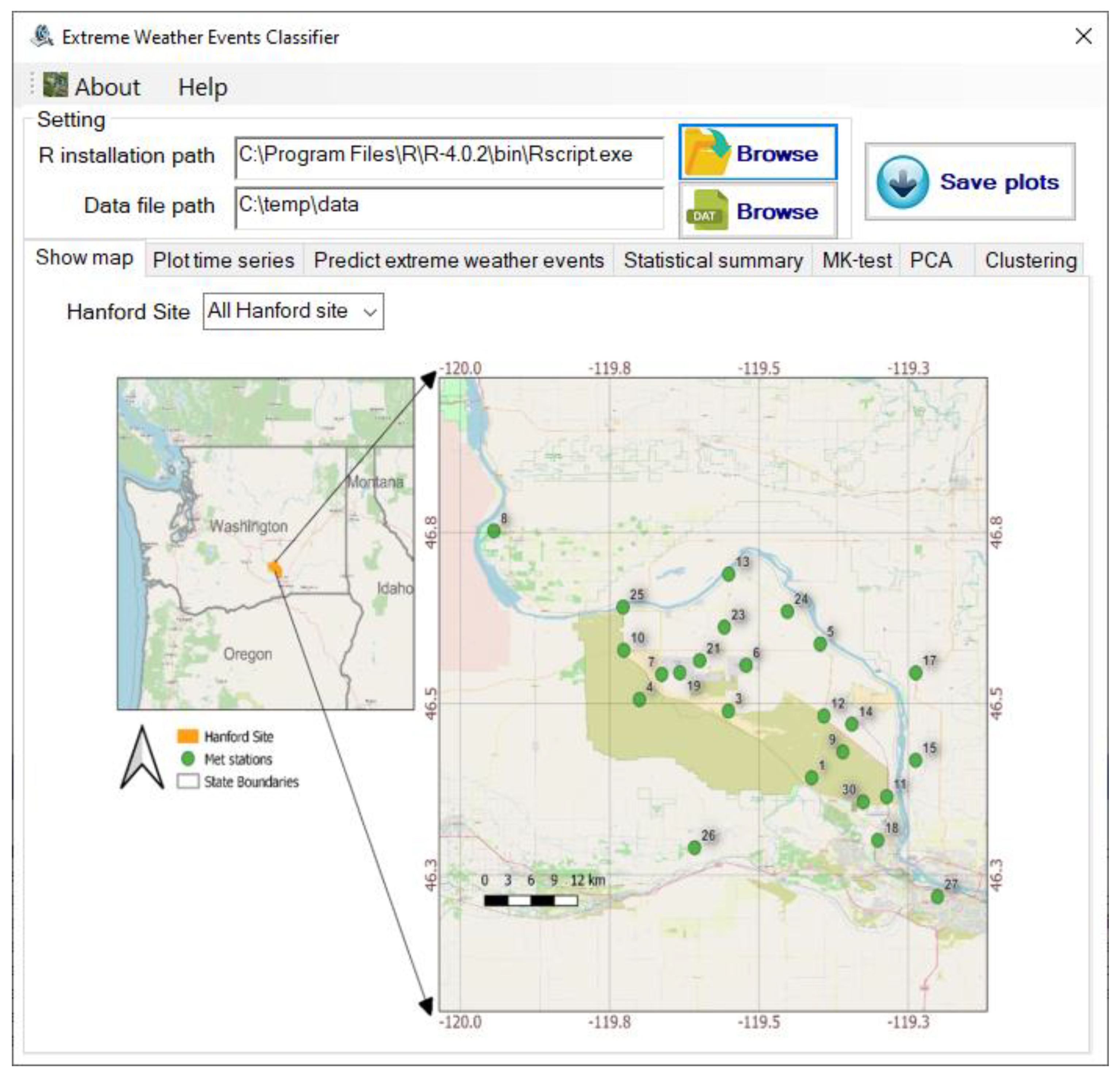
The Hanford site, the largest DOE environmental cleanup site in the United States, is located in eastern Washington state, USA (Figure 1 and Figure S1). It has 32 weather stations throughout the 1500 km2 area. The Hanford meteorological monitoring network provides a range of weather forecast products, including near real-time data from well-distributed historical meteorological and climatological data through a variety of monitoring stations. Data from 23 stations at the Hanford site was evaluated for this work. The monitoring stations are marked in green circles in Figure 1. Most of the monitoring stations are above sea level at 119 m or 120 m, with a couple at higher elevations up to 322 m.
2.2. Data Description
The meteorological data has been collected, stored, and managed through the Hanford Site monitoring program. This data can be accessed in near real-time using a linked server connection to the underlying sensor collection SQL database, which is updated every 15 min. The parameters measured at each monitoring station include temperature, wind direction, and wind speed. The 32 stations also have measurements of precipitation and air pressure. The recording units have been listed as the following: (1) temperature in Celsius (°C), (2) wind direction in radians from the north, (3) wind speed in meters per second (m/s), (4) precipitation in centimeters (cm), and (5) the air pressure in millimeters of mercury (mmHg). The Hanford region’s climate is hot during summer, with an extensive range of extremely high temperatures, often persisting at 40 °C in July and August annually. Strong wind occurs in spring, and low wind occurs in winter. Furthermore, precipitation in the Hanford region is sporadic from spring to summer. Snow is common in winter. However, the Hanford site does not collect this deposition measurement. A 10-year (2010–2019) period of data was resampled as necessary from raw data using a running average.
Data were treated to remove outliers. Additional details are provided in the Supplemental Information (SI). An example is demonstrated in Figure S2. The daily, monthly, and annual maximum and minimum data were input into the EDA framework. The mean and variance in 1-, 3-, 6-, and 12-h of each measured variable of the long-term 10-year meteorological data were included in the ML setup to classify different extreme events and evaluate their impacts on the facility operation at Hanford.
2.3. Basis for Defining Threshold and Trend Analysis
The thresholds of extreme heat and wind were adopted from criteria defined by the NOAA National Climate Data Center (NCDC, Asheville, USA). They were adjusted and used according to specific Hanford regional conditions. For example, NOAA defines sustained winds as 31 to 39 mph for at least 1 h. as windy conditions. When the heat index reaches or exceeds 40.56 °C, it is deemed excessive heat. NOAA also marks three different kinds of extreme events, namely strong wind, high temperature, and low temperature, in Benton County, where the Hanford site resides. We define the localized extreme events thresholds largely based on NOAA records (Table 1). When applying the threshold to meteorological data, about 0.7% of wind chill index records are lower than −15 °C; and about 0.5% of heat index records are greater than 38 °C. Approximately 0.65% of wind speed records are greater than 30 mph. Those percentiles are used to qualify for extreme events.
Two methods for trend analysis were adopted: namely Sen’s slope [38] and the Mann–Kendall (MK) test [39,40], to determine the representative trend of the measured parameters. The MK test is a non-parametric statistical test that can be used for detecting trends in a time series. It can identify the trend mainly based on ranks without specifying its linearity [41]. Hence, it offers robustness to non-normality and cleans data with missing values. The MK hypothesis includes the null hypothesis, where H0 refers to either a sample (i.e., measured meteorological parameter) or the independent random variables. The subsamples of each variable are independent and identically distributed over years [42].
In the null hypothesis (H0) of the MK test, data that come from a population with independent realizations are not significantly different (i.e., no trend). If the calculated p-value for a trend test is smaller than a significance level (e.g., 0.05), the null hypothesis is rejected (i.e., the trend is significant). The MK method is well-known for assessing the significance of trends in hydroclimatic time series data, such as rainfall, temperature, and streamflow [43,44,45,46,47].
The Seasonal Kendall (SK) test, an extension of the MK test, is usually adopted when the data are collected with expected monotonic trends during different seasons [48,49]. Seasonality may exist for long-term data with different distributions over months, quarters, or seasons of many years. In addition, using Sen’s slope is another classical method to quantify the trend by calculating the slope of the parameter trends through pairs of sample points. It is a non-parametric technique as an alternative to the linear models using the median of the slopes. This trend estimation is robust to outliers with a breakdown point of 0.29 and can be computed efficiently [50,51,52].
2.4. RF Classification
An RF is an ensemble ML algorithm using a collection of decision trees as base classifiers [26], i.e., , where the are independent and identically distributed random vectors, and x the input vector that each tree casts a unit vote for the most popular class. RF is robust to categorical and numerical data types. The prediction of the RF is obtained by a majority vote from the individual decision tree. To reduce the variance of a decision tree and achieve the stability of classifiers with high accuracy, a bootstrap aggregating technique (bagging) was applied to ensure random and uniform resampling from the full training dataset with replacement [53,54]. The input features give an equal weight during split using resampling instead of reweighting [26]. Each tree has a set of internal nodes and leaves developed by user-defined parameters, including the number of trees in the ensemble and the number of predictive variables used to split the nodes. Any tree is allowed to grow to the maximum possible depth with a given combination of features to improve tree-based model performance [53,55]. In the internal nodes, the selected feature is used to make decisions in each individual tree and the correlation between any two trees to evaluate the generalization error. The convergence of the generalization error provides a means to estimate the required number of trees. The Gini index, a popular quantity for splitting selection, measures the frequency at which any features of the dataset will be mislabeled when it is randomly labeled. We collect how, on average, it decreases the impurity for each measured parameter. Feature importance (FI) helps to understand the RF models because the importance score provides insight into features that are the most and least important to the model when making a prediction. The FI score can help feature selection. Additionally, it can be used to improve the predictive model by facilitating feature selection [56].
2.5. GUI Development for Rapid Assessment
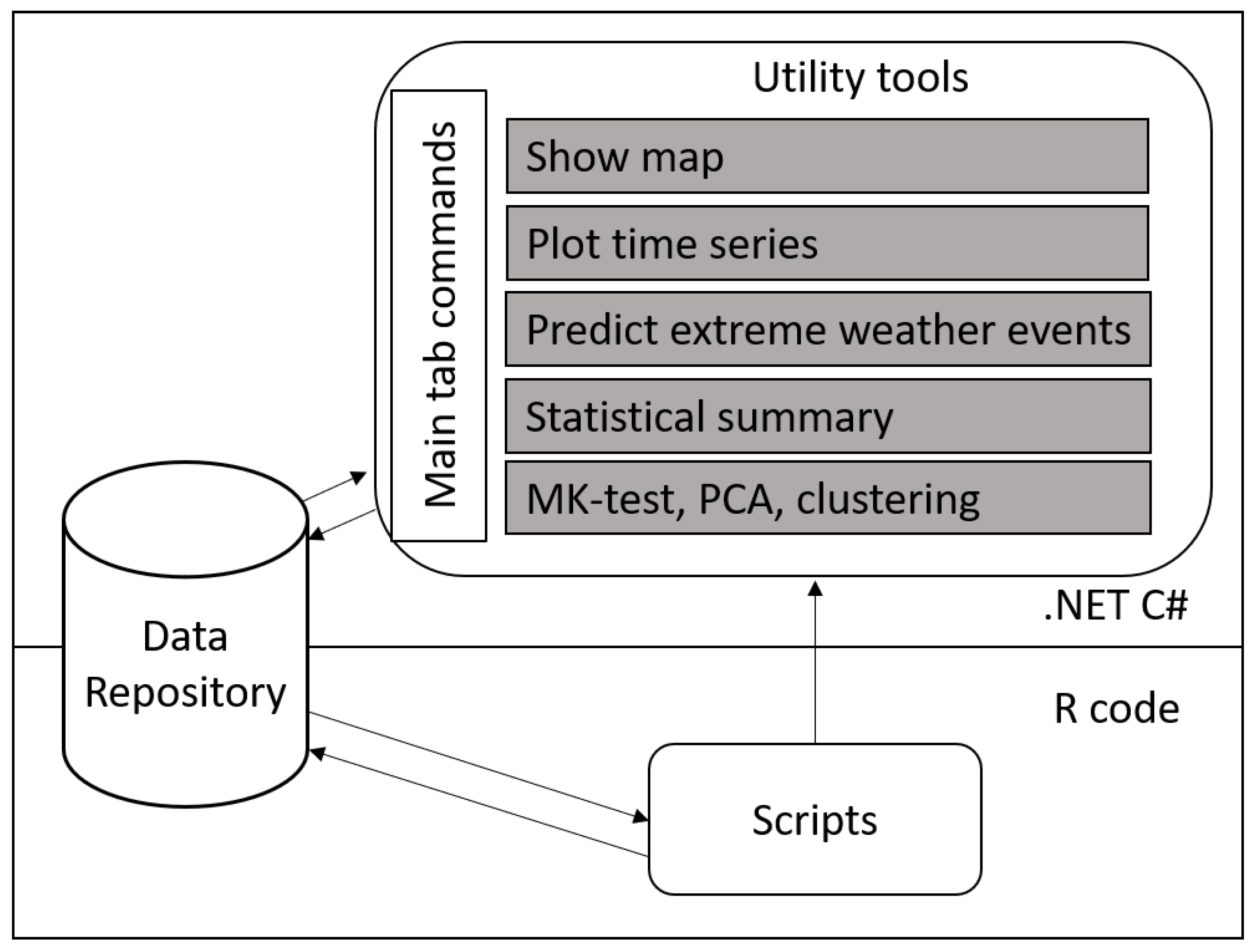
The EWEC is an integrated suite of science-based tools with a user-friendly interface. Code for the development of this tool is managed and available via git through the PNNL data repository (Figure 2). Built with .NET C#, EWEC incorporates R scripts to perform data analyses and plotting. It uses historical meteorological data collected at monitoring stations to analyze and characterize weather extreme events. EWEC enables users to analyze data, classify extreme weather events, and develop and validate weather extreme prediction models. However, if needed, users can flexibly adapt to any new formats by adjusting the input parameters for the pre-created R scripts. To use all the features of EWEC, R software is required to install R packages, such as dplyr, lubridate, plyr, and plotrix. After completing all those processes, users need to set the R installation path and data file locations to use EWEC. EWEC is free and available to all users upon request.
3. Results
3.1. Threshold for Extreme Events
Winds with relatively low speed but lasting longer than 3 h occurred more frequently in winter compared to other seasons based on the 10-year meteorological data. In addition, low-speed winds lasting longer than 48 h, and even up to 10 days, were observed in winter. If hazardous particles were released during such low wind or stagnant periods, it is less likely they would be transported downwind over longer distances throughout the Hanford site. In contrast, high-speed winds occurred more frequently in the spring and summer compared to other seasons. The summer season in the Hanford region is typically dry with little precipitation. The longest record without precipitation was 186 days from station 5 starting in May 2013 (See Table S2). Similarly, station 7 also had a period without rainfall which lasted 111 days at the same time. Station 5 had more periods without precipitation than other stations. A long period without precipitation accompanied by low humidity could lead to wildfires, a hazardous event for the Hanford site area. Understanding and predicting these conditions are therefore critical for environmental monitoring and remediation. Figure S3 provide additional information on the frequency of low wind and high wind events.
3.2. Seasonal MK Test and Sen’s Slope Analysis
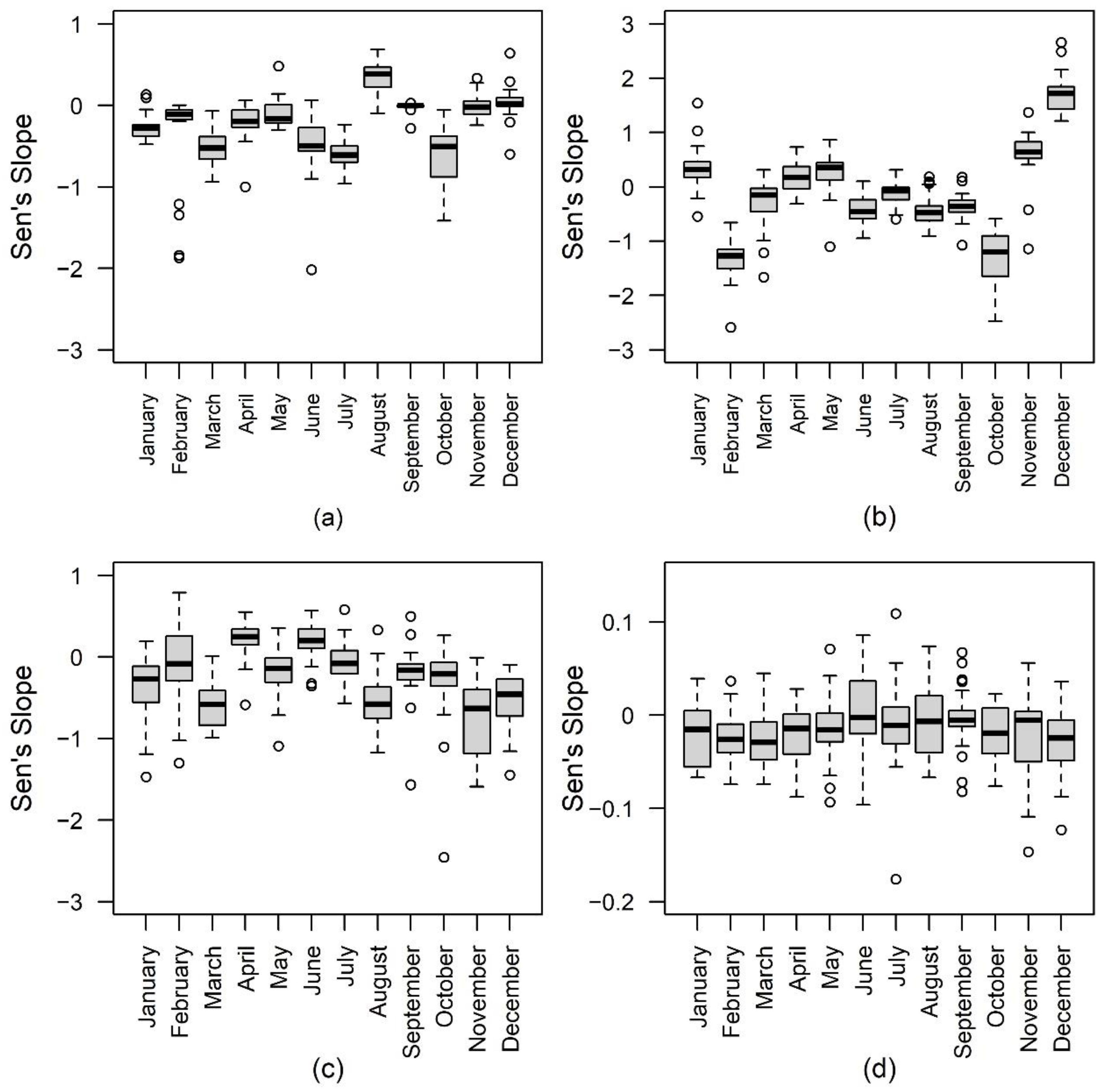
A seasonal MK test was applied for identifying the monotonic trend which could occur in different seasons. To extract the trending magnitude, Sen’s slope was used to measure the slope of a regression line fit using observed trends among the sample periods. For example, if Sen’s slope is positive, it indicates an increasing trend. In contrast, a negative Sen’s slope implies a decreasing trend. Both maximum and minimum monthly temperature and wind speed were extracted in the MK test to highlight trends in the two types of extreme directions in different seasons in Hanford. Temperature and wind speed values analyzed in Sen’s slope analysis can be interpreted as down-trending or decreasing over the 10 years when values are less than zero. Similarly, Sen’s slope results can be interpreted as up-trending or increasing over the 10-year period when values are greater than zero (Figure 3).
The Sen’s slope box plot of the maximum monthly temperature is shown in Figure 3a. The trend of the maximum monthly temperature has decreased over the past decade. However, the trend of maximum monthly temperature increased in August. The values of Sen’s slopes are close to 0. The result indicates that the variation of temperature in September is statistically insignificant. This result suggests that summers persist until August and that the maximum temperature is increasing. The Sen’s slope box plot of the minimum monthly temperature is depicted in Figure 3b. The monthly minimum temperature increases during winter. February and October’s minimum and maximum monthly temperatures tend to go down, which suggests that transitional seasonal high and low temperatures are lower than in previous years.
The Sen’s slope box plot of the maximum monthly wind speed is demonstrated in Figure 3c. The positive values of Sen’s slope represent the increasing trend, and the negative values of Sen’s slope the decreasing trend. The trend of the maximum monthly wind speed decreases in January, March, November, and December, respectively, among most stations. The variations in September among most stations are minor. However, the outliers located outside the whiskers of the box plot in September are noticeable, which identify the strong variability in the extreme values. The Sen’s slope box plot of the minimum wind speed is presented in Figure 3d. The range of Sen’s slopes is from −0.15 to 0.1, which indicates that variations of the minimum wind speed are insignificant. Almost all the box plot’s medium values are close to 0. In general, wind speed becomes stronger in April and June. The light air conditions do not change significantly at the same time, unlike the wind conditions.
Distinct seasonal trends were observed with respect to the intensity and duration of wind speed and temperature, having important ramifications for atmospheric dispersion and natural hazard events. Results from Sen’s slope analysis indicate that for most months, maximum monthly temperatures have been trending downward over the past 10 years. However, August temperatures showed a notable increase in maximum temperatures over the last 10 years. February, October, and December exhibited a strong trend in minimum temperatures over the 10-year period. Other months exhibited minor changes over the 10-year period.
3.3. Features before, during, and after an Extreme Event
Wind direction, wind speed, temperature, precipitation, and temperature were characterized before and after a heatwave and strong wind events in 3-, 6- and 12-h. bins, which were used to represent an extreme event in the following methods.
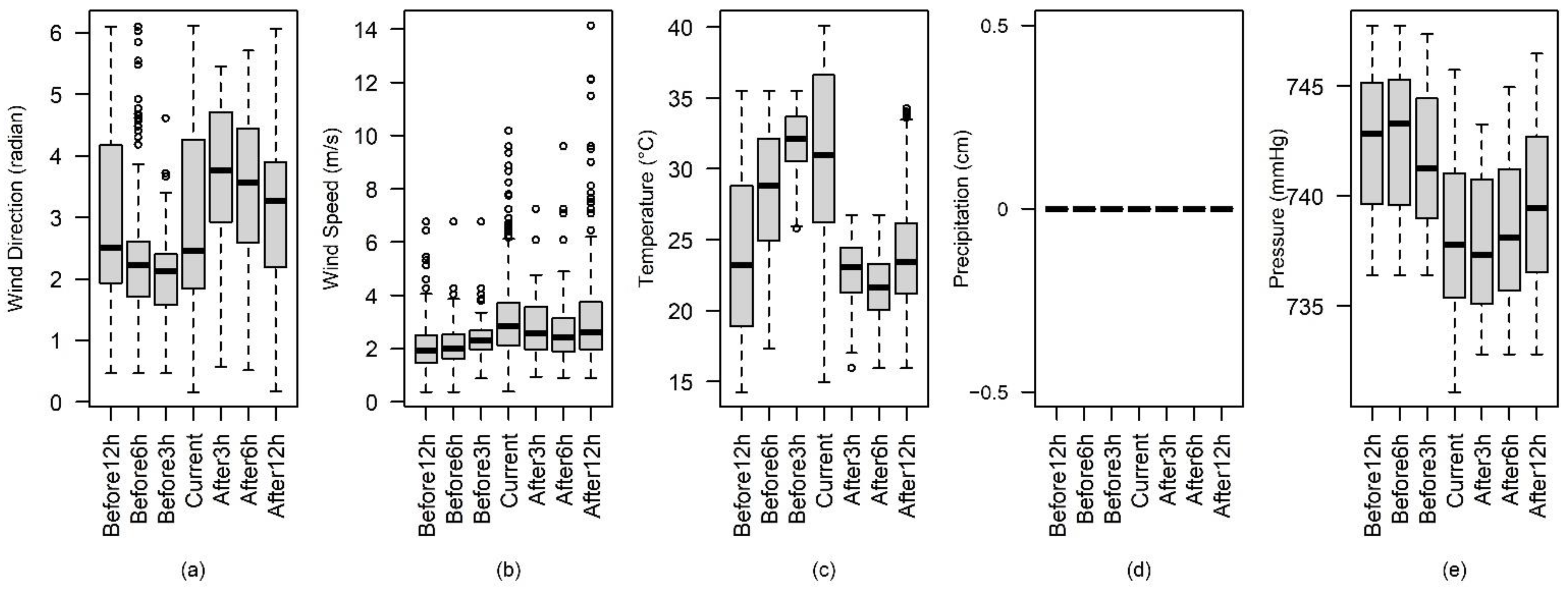
Heatwaves typically occur in the summer, characterized by persistent high temperatures. The diurnal atmosphere pressure variation is approximately 0.6 mm Hg during normal conditions for a mid-latitude region such as Hanford [57]. If a severe event happens, pressure changes accordingly. The box plots of meteorological measurement data 12-, 6-, and 3-h. before the heatwave event, data during an event, and data 3-, 6-, and 12-h. after the heatwave, are represented in Figure 4. The wind speeds observed in summer are not high. Based on the observed data and identified events, when wind speed increases, pressure decreases. Temperature increases when a heatwave occurs (see Figure 4c). Meanwhile, pressure decreases slightly, and wind speed increases. The wind direction may have a 12-h. cycle. The wind direction observations from 12-h. before, during, and 12-h. after range from close to 0 (the lower bound) to more than 6 radians (the higher bound).
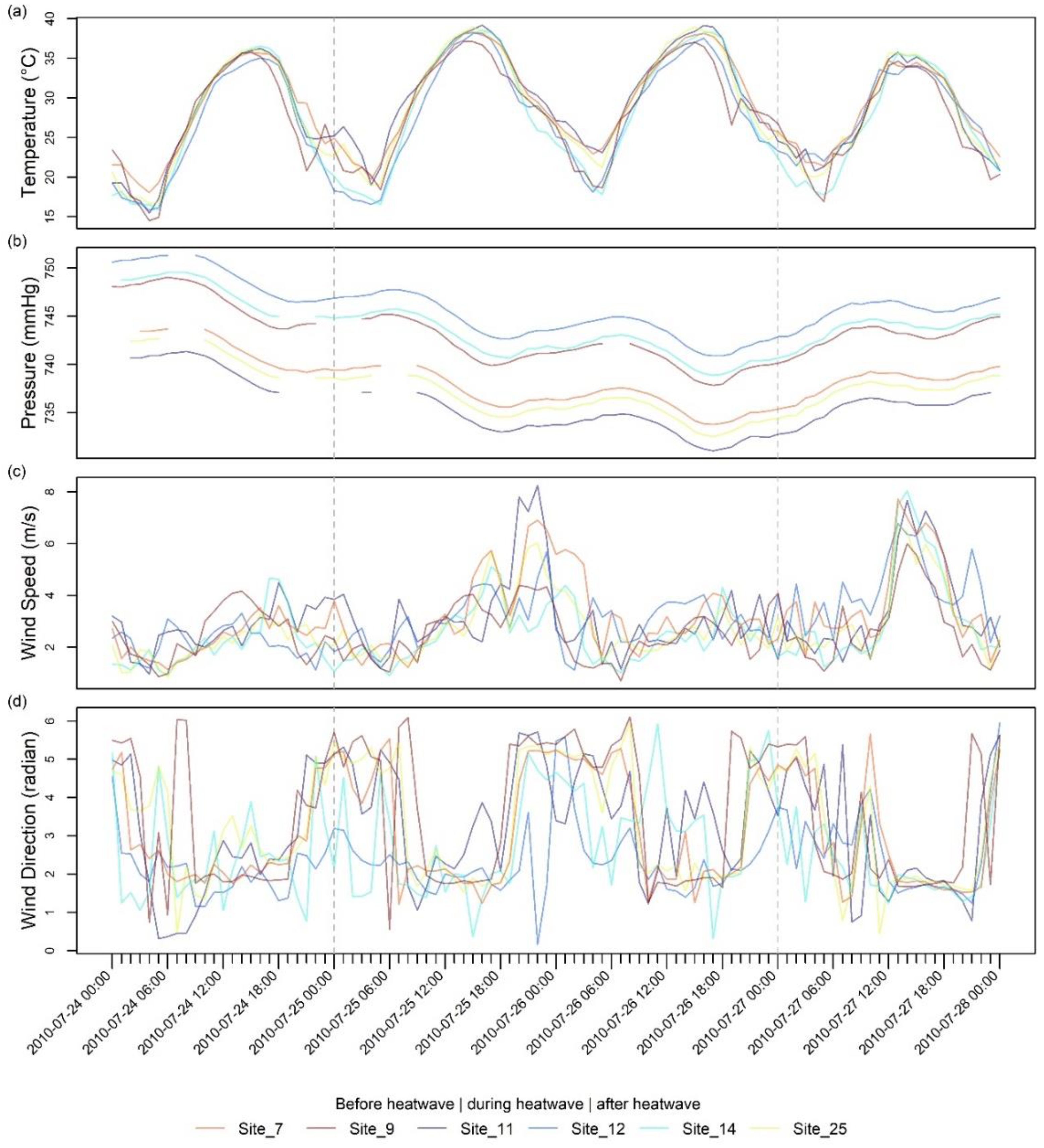
A selected time series of meteorological measurements during the heatwave episode is displayed in Figure 5. Six stations are selected to highlight the temporal change in temperature and pressure. This exercise is limited due to data availability because only 6 out of the 32 weather stations have measured the complete meteorological variables. A heatwave does not significantly impact wind speed or wind direction. The temperatures of 25 and 26 July of 2010 were higher than those before and after heatwave events. The temperature was high during the advent of heatwave events, and it remained high continuously. There was an anticorrelation between temperature and pressure. When temperatures went up (Figure 5a), pressures went down (Figure 5b). During the heatwave event, pressure was lower than before and after such an event. This finding can help us form the primary applications of weather-driven extreme events that may complicate site operation when dealing with hazard transport and dispersion. The wind speed plot (Figure 5c) shows that the wind speed is low during the heatwave period. The lower wind speed could not dissipate heat efficiently and may have been a factor for the observed prolonged heatwave events in Hanford during summers. High pressure conditions were associated with low wind speeds [58]. Figure 5d illustrate that, in general, the wind direction is high in radians at nighttime. As only three monitoring stations have complete observed parameters, it is expected that these results may not provide a full understanding of the cause and relationship of the heatwave occurrences. The key implication is that meteorological data must be fully accessible before further investigation. The approach illustrated here serves this purpose.
3.4. EWEC GUI for Rapid Assessment
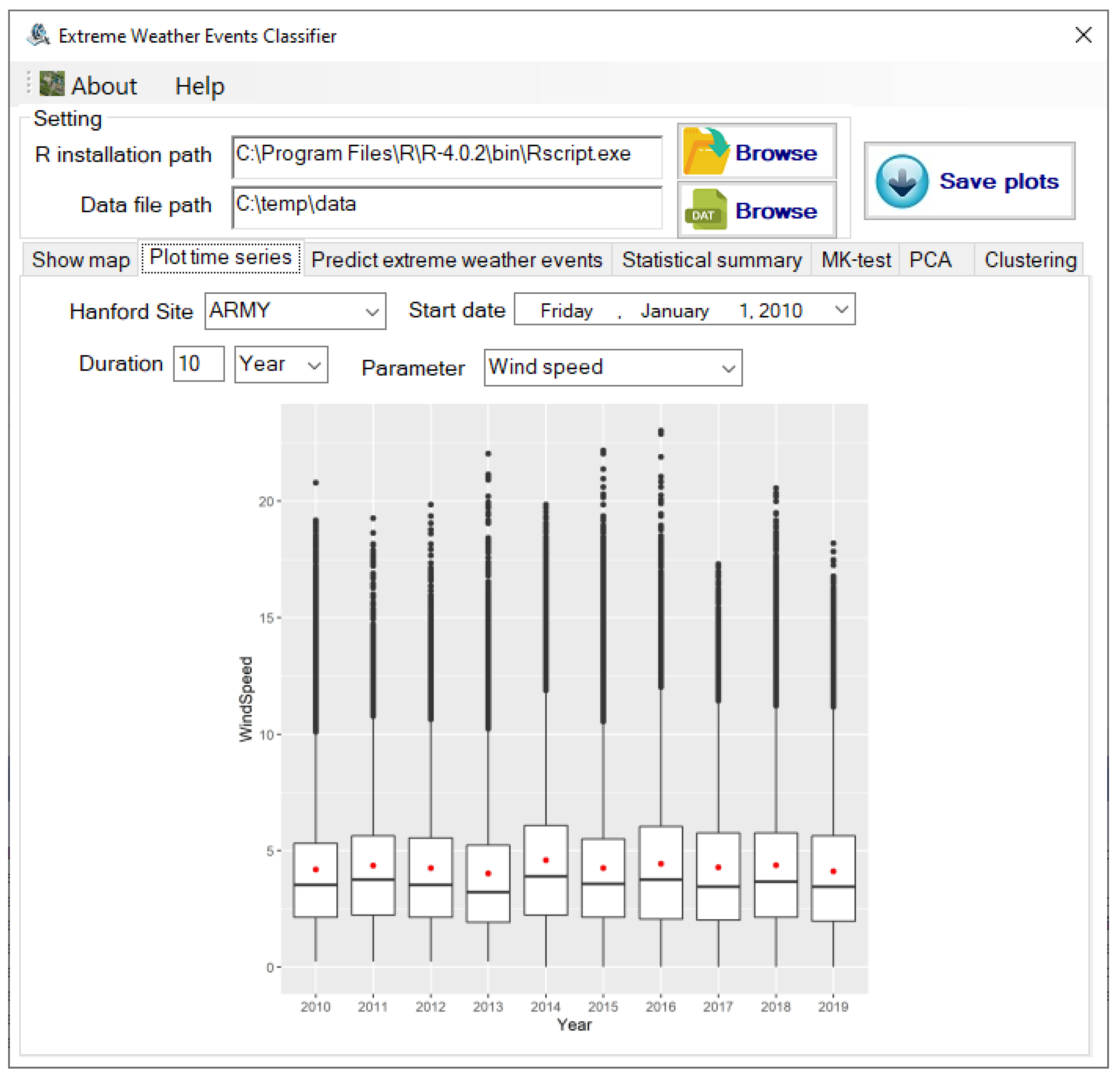
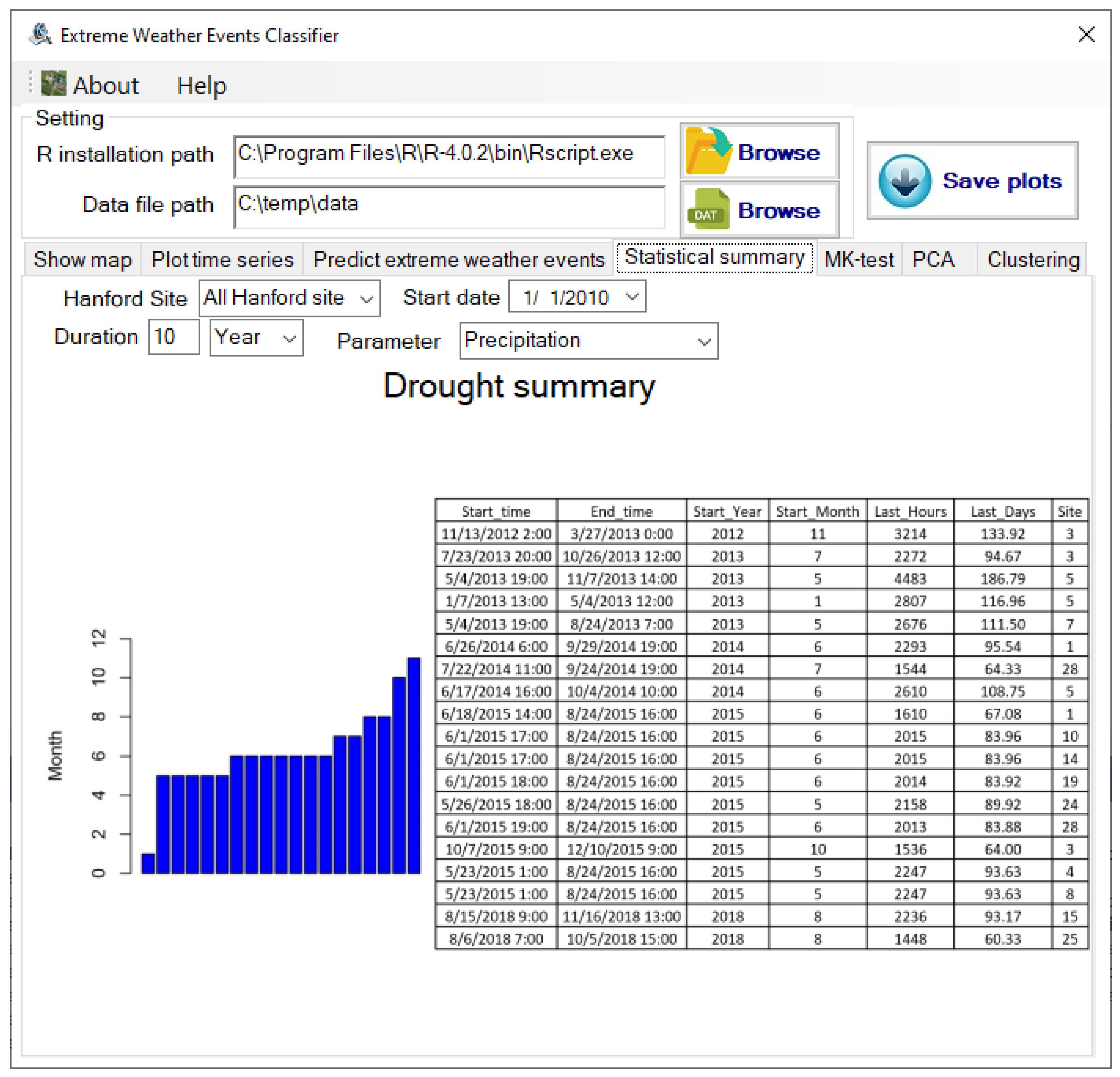
Currently, EWEC supports comma-separated value (CSV) data files, which contain data in the order of timestamp, wind direction, wind speed, temperature, precipitation, and pressure. EWEC contains seven major components corresponding to the seven tabs in the user interface. The “Show map” component is used to show the geolocations of the user-picked stations and the corresponding weather stations. The “Plot time series” component is used to plot a meteorological time series for user-selected stations, parameters, and time periods. For example, the plot of wind speed time series from 2010 to 2019 in the ARMY station is illustrated in Figure 6. The “Predict extreme weather events” component is used to detect extreme weather events for the meteorological dataset using regional specified thresholds, which can vary if moving to different regions. The “Statistic summary” component is used to provide summary information of the monitoring data, including different types of wind, drought/precipitation, temperature, and a strong variation of pressure change. The drought information, for example, when choosing 60 days as the threshold for all Hanford monitoring stations from 2010 to 2019, can be seen in Figure 7. According to the data analysis, we can conclude that 2013, 2014, and 2015 had more maximum drought periods than other years, and drought usually happened in summer. The “MK-test” component is used to analyze the trending non-stationarity of weather attributes. The “PCA” component is used to detect heatwaves and strong wind events for the selected period for the selected stations. The “Clustering” component is used to detect the similarities of each parameter for the selected period among all stations.
3.5. Extreme Event Classification
EDA results suggest that heatwave events are seasonally triggered, often occurring in summer. Strong wind events occurred in all seasons but were more prevalent in spring. We summarized different types of extreme events and labeled them individually using the defined thresholds presented in Table 1. We used the classification framework to predict events in the Hanford region without records for other kinds of extreme events such as strong winds, heatwaves, and winter storms. In this ML classification setup, if an extreme event occurs in a specific month, the data from this month will be converted into ML input data. Data collection is not complete among all stations. For example, station 11 had sufficient data to build the ML models, and it was selected for ML classification model development regarding two extreme event types, namely, heatwaves and strong wind. It is found that meteorological data have noticeable changes before an extreme event. The mean and variance of the previous 1-, 3-, 6-, and 12-h. data are generated based on the monitoring data for each current hour and variables. Data were randomly split into training data (70%), validation data (15%), and testing data (15%) for both the heatwave and strong wind RF models.
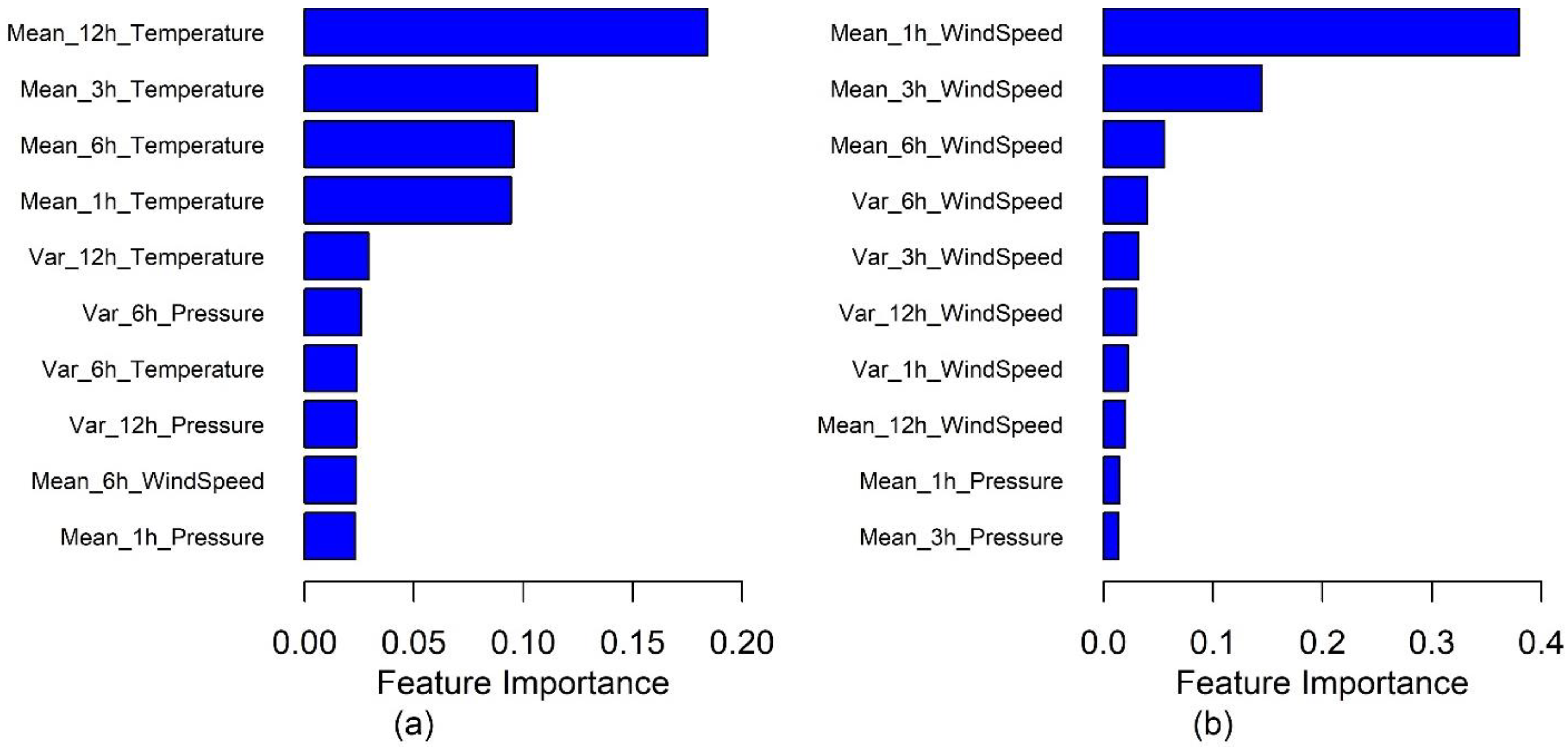
The top 10 FI plots of the heatwave model and the strong wind model are presented in Figure 8a,b, respectively. Figure 8a demonstrate that the past 12-, 6-, 3-, and 1-h. temperatures are essential indicators for heatwaves. Pressure-related parameters, such as the variation of the past 12-h. temperature and the past 6-h. pressure, also contribute to the heatwave RF model. The average temperature of the past 12 h is the dominant factor in the heatwave model, and FIs of the average 1-, 3-, and 6-h. temperature are comparable.
Our RF model results show that persistent high temperatures during a longer time window, i.e., the mean temperature in a 12-h. window, greatly impacts heatwave events. This indicates that a heatwave is a climate phenomenon affected by prolonged high temperatures. The FI of the strong wind model is demonstrated in Figure 8b. In general, the variations of meteorological measurements are less important than the mean values. The past 1-h. wind speed is the dominant factor, and its importance is much higher than the rest of the parameters. Our results suggest that short-time wind speed is more important in the strong wind model.
RF classification models were developed to capture non-heat wave periods and periods with strong wind speeds using the aforementioned training, validation, and testing datasets. The RF models return predictions by probability. In this work, we use 0.5 as the threshold to evaluate the predicted probability. A false positive error means that the predicted probability is greater than 0.5, and the actual probability is less than or equal to 0.5. Conversely, a false negative error indicates that the predicted probability is equal to or less than 0.5 and the actual probability is greater than 0.5. The actual and forecast results of the heatwave and strong wind RF models are shown in Table 2, respectively. Both models have reached high accuracy on event classification (see Table S3). The misclassified classes, including both false negative and false positive errors, are comparable concerning the testing results of heatwave extreme events. The strong wind model tends to classify more false negatives. These misclassified samples could be caused by the variation in a strong wind which leads, incorrectly, to an association with the positive error. In addition, the patterns of the sampled data may be similar, which cannot be distinguished by the classifier.
4. Discussion
Both EDA analysis and RF classification were applied to study long-term meteorological data in Hanford in this study. The Sen’s slope variation of the maximum monthly temperature is smaller than that of the minimum monthly temperature, according to the MK test results. The maximum monthly temperature increases among most stations are not as significant as the minimum monthly temperature. Minimum temperatures at all stations increase in winter, indicating that the lower monthly temperatures increase. Sen’s slopes of the maximum monthly temperature at most stations are around 0. This finding suggests that most of the minimum temperature increases and the maximum temperature remains at a level comparable to historical records. These findings imply that extremely high temperatures will increase in the future, with all other assumptions remaining the same. Our results show that ML, specifically RF models, can assist the mechanistic/predictive model development by utilizing existing decadal records and adding more predicted features.
Additionally, Table S1 gives the summary of the low wind speed lasting more than 5 days in the Hanford area. Low wind speed is another extreme regional event in summer. Wildfires always occur in the Pacific Northwest in summer, and low wind speed makes the smoke stagnate and sit in the Columbia basin area. Prolonged stagnation has often led to hazardous conditions for outdoor activities, including performing job functions on site. Therefore, the ability to predict and prevent adverse exposure conditions is valuable for improving site operations. Moreover, particle release in low wind scenarios may cause more unpredictable damages due to low visibility. This type of extreme event warrants further investigation.
Ongoing analyses are being conducted upon historical meteorological datasets with different frequencies in Hanford to validate the RF models. Those datasets include data acquired and streamed at different intervals, such as every 15-min or hourly, near real-time. Beyond model validation, potential future upgrades being considered include data imported from other meteorological monitoring sites to make this approach feasible for applications elsewhere.
5. Conclusions
Meteorological data for a period spanning 10 years were investigated to study the local climate change trend at the Hanford site. EDA was used to study the weather pattern and capture trends indicative of extreme weather that impacts site operations. RF classification was used to classify extreme weather conditions such as strong winds and heatwaves. The heatwave and the strong wind RF models were developed and investigated. The acceptance performance of the RF models was validated. The strong wind model was shown to be sensitive to the past 1 h wind speed. The heatwave model relies more on the average temperature of the past 12-, 3-, and 6-h, respectively.
Extreme events are becoming more common at the Hanford Site. The extreme events of heatwaves and strong wind were studied as the most impactful and representative scenarios in this work. Higher risks in site operation (e.g., failure in ventilation systems, power outage) may be caused by or related to prolonged heatwaves. Our results suggest that a heatwave is a cumulative phenomenon. Thus, it is possible to use the previous days’ temperature or pressure to help predict heatwave events. Strong and low wind events are other types of extreme events that need investigation. Wind speed can change in a short time, and it is affected by site temperature and pressure. Low wind speed has an inconsequential effect on the accidental release and subsequent dispersion of hazardous particles, as it tends to prevent particle transport downwind away from the site. Therefore, studying extreme events using long-term big meteorological data in Hanford is important to guide site operations. The development of the EWEC GUI provides a user-friendly means to process a large amount of meteorological data using statistical analysis and EDA. It gives an example of a practical tool for DOE sites. More importantly, this work provides a new means of long-term meteorological data assessment using ML, particularly RF models, to enable sensible characterization and lead to improvement of the safety analysis standard warranted for the safeguarding of the DOE facilities, personnel, and operations.
Supplementary Materials
The following are available online at https://www.mdpi.com/article/10.3390/atmos13010136/s1, Algorithm S1: MK test. Algorithm S2: Random Forest. Algorithm S3: Outlier detection. Figure S1: Location of the Hanford Site of the Columbia River and meteorological stations. Figure S2: Data outlier analysis of pressure measurement. Figure S3: Frequency summary of low wind speed of all sites monthly lasting more than (a) 3 h and (b) 48 h. Similarly, frequency summary of high wind speed of all sites monthly lasting more than (c) 3 h and (d) 48 h. Figure S4: The PCA biplots showing (a) no heatwave and (b) heatwave events among all stations over 10 years. Figure S5: The PCA biplots showing (a) no strong wind and (b) strong wind events among all stations over 9 years. Figure S6: Time series plots of the day before, during, and after the strong wind event: (a) temperature, (b) pressure, (c) wind speed, and (d) wind direction. Figure S7. The F1 results of the RF models parameters tuning under different trees: (a) the strong wind and (b) the heatwave model. Figure S8. The accuracy of RF models parameter tuning under different minimum sample splits: (a) the strong wind and (b) the heatwave model. Figure S9. The accuracy of RF models parameter tuning under different minimum sample leaves: (a) the strong wind and (b) the heatwave model. Table S1: Summary of the low wind period. Table S2: Summary of the no precipitation period. Table S3. The model evaluation table of Table 2.
Author Contributions
Conceptualization, X.-Y.Y. and H.R.; methodology, H.R., H.H., H.Z. and X.-Y.Y.; software, H.H., H.Z. and H.R.; validation, H.Z. and H.R.; formal analysis, H.R., H.Z. and X.-Y.Y.; investigation, H.R., H.Z. and X.-Y.Y.; resources, H.R. and X.-Y.Y.; data curation, P.R.; writing—original draft preparation, H.Z., H.R., H.H. and X.-Y.Y.; writing—review and editing, H.R., X.-Y.Y., H.H. and P.R.; supervision, X.-Y.Y.; project administration, X.-Y.Y.; funding acquisition, X.-Y.Y. All authors have read and agreed to the published version of the manuscript.
Funding
The authors are grateful for the programmatic support from the Department of Energy (DOE) NNSA AU31 program. The opinions expressed are solely based on the research results of the authors. Computational resources are from R and Python.
Institutional Review Board Statement
Not applicable.
Informed Consent Statement
Not applicable.
Data Availability Statement
The data presented in this study are available on request from the corresponding author. The data are not publicly available because they are germane to the Hanford site operation.
Acknowledgments
Pacific Northwest National Laboratory (PNNL) is operated for the U.S. DOE by Battelle Memorial Institute under Contract No. DE-AC05-76RL01830.
Conflicts of Interest
The authors declare no conflict of interest.
References
- Albeverio, S.; Jentsch, V.; Kantz, H. Extreme Events in Nature and Society; Springer Science & Business Media: Berlin/Heidelberg, Germany, 2006; pp. 1–9. [Google Scholar]
- Dehghanian, P.; Zhang, B.; Dokic, T.; Kezunovic, M. Predictive Risk Analytics for Weather-Resilient Operation of Electric Power Systems. IEEE Trans. Sustain. Energy 2019, 10, 3–15. [Google Scholar] [CrossRef]
- Otto, F.E.L.; Philip, S.; Kew, S.; Li, S.; King, A.; Cullen, H. Attributing high-impact extreme events across timescales—a case study of four different types of events. Clim. Change 2018, 149, 399–412. [Google Scholar] [CrossRef] [Green Version]
- Katz, R.W.; Brown, B.G. Extreme events in a changing climate: Variability is more important than averages. Clim. Change 1992, 21, 289–302. [Google Scholar] [CrossRef]
- Staid, A.; Guikema, S.D.; Nateghi, R.; Quiring, S.M.; Gao, M.Z. Simulation of tropical cyclone impacts to the US power system under climate change scenarios. Clim. Change 2014, 127, 535–546. [Google Scholar] [CrossRef]
- Marx, J.D.; Cornwell, J.B. The importance of weather variations in a quantitative risk analysis. J. Loss Prev. Process Ind. 2009, 22, 803–808. [Google Scholar] [CrossRef]
- Bubbico, R. A statistical analysis of causes and consequences of the release of hazardous materials from pipelines. The influence of layout. J. Loss Prev. Process Ind. 2018, 56, 458–466. [Google Scholar] [CrossRef]
- CCPS. Guidelines for Siting and Layout of Facilities; Wiley: Hoboken, NJ, USA, 2018; pp. 59–62. [Google Scholar]
- Stephenson, D.B.; Diaz, H.F.; Murnane, R.J. Definition, diagnosis, and origin of extreme weather and climate events. In Climate Extremes and Society; Cambridge University Press: Cambridge, UK, 2008; Volume 340, pp. 11–23. [Google Scholar]
- Huth, R.; Beck, C.; Philipp, A.; Demuzere, M.; Ustrnul, Z.; Cahynova, M.; Kysely, J.; Tveito, O.E. Classifications of atmospheric circulation patterns: Recent advances and applications. ANNALS N. Y. Acad. Sci. 2008, 1146, 105–152. [Google Scholar] [CrossRef]
- Hershfield, D.M. On the Probability of Extreme Rainfall Events. Bull. Am. Meteorol. Soc. 1973, 54, 1013–1018. [Google Scholar] [CrossRef]
- Tukey, J.W. Exploratory Data Analysis; Addison-Wesley: Reading, MA, USA, 1977; Volume 2. [Google Scholar]
- DOE-STD-3009-2014; Preparation of Nonreactor Nuclear Facility Documented Safety Analysis; DOE: Washington, DC, USA, 2014.
- Hodge, V.J.; Austin, J. A survey of outlier detection methodologies. Artif. Intell. Rev. 2004, 22, 85–126. [Google Scholar] [CrossRef] [Green Version]
- Rousseeuw, P.J.; Leroy, A.M. Robust Regression and Outlier Detection; John Wiley & Sons: Hoboken, NJ, USA, 2005; Volume 589. [Google Scholar]
- Maimon, O.; Rokach, L. Outlier detection. In Data Mining and Knowledge Discovery Handbook; Maimon, O., Rokach, L., Eds.; Springer: Berlin/Heidelberg, Germany, 2005; pp. 131–146. [Google Scholar]
- Akouemo, H.N.; Povinelli, R.J. Time series outlier detection and imputation. In Proceedings of the 2014 IEEE PES General Meeting|Conference & Exposition, National Harbor, MD, USA, 27–31 July 2014; pp. 1–5. [Google Scholar]
- Zhang, M.H.; Li, X.; Wang, L.L. An Adaptive Outlier Detection and Processing Approach Towards Time Series Sensor Data. IEEE Access 2019, 7, 175192–175212. [Google Scholar] [CrossRef]
- Wang, H.Z.; Bah, M.J.; Hammad, M. Progress in Outlier Detection Techniques: A Survey. IEEE Access 2019, 7, 107964–108000. [Google Scholar] [CrossRef]
- Camizuli, E.; Carranza, E.J. Exploratory data analysis (EDA). Encycl. Archaeol. Sci. 2018, 1–7. [Google Scholar] [CrossRef]
- Ren, F.M.; Trewin, B.; Brunet, M.; Dushmanta, P.; Walter, A.; Baddour, O.; Korber, M. A research progress review on regional extreme events. Adv. Clim. Change Res. 2018, 9, 161–169. [Google Scholar] [CrossRef]
- Farnham, D.J.; Doss-Gollin, J.; Lall, U. Regional Extreme Precipitation Events: Robust Inference From Credibly Simulated GCM Variables. Water Resour. Res. 2018, 54, 3809–3824. [Google Scholar] [CrossRef]
- Joseph, B.; Wang, F.H.; Shieh, D.S.S. Exploratory Data Analysis: A Comparison of Statistical-Methods with Artificial Neural Networks. Comput. Chem. Eng. 1992, 16, 413–423. [Google Scholar] [CrossRef]
- Singh, K.; Nagpal, R.; Sehgal, R. Exploratory Data Analysis and Machine Learning on Titanic Disaster Dataset. In Proceedings of the 2020 10th International Conference on Cloud Computing, Data Science & Engineering (Confluence), Noida, India, 29–31 January 2020; pp. 320–326. [Google Scholar]
- Jones, Z.M.; Linder, J.F. edarf: Exploratory Data Analysis using Random Forests. J. Open Source Softw. 2016, 1, 92. [Google Scholar] [CrossRef] [Green Version]
- Breiman, L. Random forests. Mach. Learn. 2001, 45, 5–32. [Google Scholar] [CrossRef] [Green Version]
- Jaiswal, J.K.; Samikannu, R. Application of random forest algorithm on feature subset selection and classification and regression. In Proceedings of the 2017 World Congress on Computing and Communication Technologies (WCCCT), Tiruchirappalli, India, 2–4 February 2017; pp. 65–68. [Google Scholar]
- Lee, S.; Choi, H.; Cha, K.; Chung, H. Random forest as a potential multivariate method for near-infrared (NIR) spectroscopic analysis of complex mixture samples: Gasoline and naphtha. Microchem. J. 2013, 110, 739–748. [Google Scholar] [CrossRef]
- Friedman, J.H. Stochastic gradient boosting. Comput. Stat. Data Anal. 2002, 38, 367–378. [Google Scholar] [CrossRef]
- Friedman, J.H. Greedy function approximation: A gradient boosting machine. Ann. Stat. 2001, 29, 1189–1232. [Google Scholar] [CrossRef]
- Ren, H.; Song, X.; Fang, Y.; Hou, Z.J.; Scheibe, T.D. Machine Learning Analysis of Hydrologic Exchange Flows and Transit Time Distributions in a Large Regulated River. Front. Artif. Intell. 2021, 4, 648071. [Google Scholar] [CrossRef]
- Nawar, S.; Mouazen, A.M. Comparison between Random Forests, Artificial Neural Networks and Gradient Boosted Machines Methods of On-Line Vis-NIR Spectroscopy Measurements of Soil Total Nitrogen and Total Carbon. Sensors 2017, 17, 2428. [Google Scholar] [CrossRef]
- Zhang, Y.; Haghani, A. A gradient boosting method to improve travel time prediction. Transp. Res. Part C Emerg. Technol. 2015, 58, 308–324. [Google Scholar] [CrossRef]
- Booker, D.J.; Snelder, T.H. Comparing methods for estimating flow duration curves at ungauged sites. J. Hydrol. 2012, 434, 78–94. [Google Scholar] [CrossRef]
- Snelder, T.H.; Datry, T.; Lamouroux, N.; Larned, S.T.; Sauquet, E.; Pella, H.; Catalogne, C. Regionalization of patterns of flow intermittence from gauging station records. Hydrol. Earth Syst. Sci. 2013, 17, 2685–2699. [Google Scholar] [CrossRef] [Green Version]
- Kaminska, J.A. A random forest partition model for predicting NO2 concentrations from traffic flow and meteorological conditions. Sci. Total Environ. 2019, 651, 475–483. [Google Scholar] [CrossRef]
- O’Gorman, P.A.; Dwyer, J.G. Using Machine Learning to Parameterize Moist Convection: Potential for Modeling of Climate, Climate Change, and Extreme Events. J. Adv. Model. Earth Syst. 2018, 10, 2548–2563. [Google Scholar] [CrossRef] [Green Version]
- Sen, P.K. Estimates of the Regression Coefficient Based on Kendall’s Tau. J. Am. Stat. Assoc. 1968, 63, 1379–1389. [Google Scholar] [CrossRef]
- Mann, H.B. Nonparametric Tests against Trend. Econometrica 1945, 13, 245–259. [Google Scholar] [CrossRef]
- Kendal, M.G. Rank Correlation Methods. Br. J. Stat. Psychol. 1956, 9, 68. [Google Scholar] [CrossRef]
- Pingale, S.M.; Khare, D.; Jat, M.K.; Adamowski, J. Spatial and temporal trends of mean and extreme rainfall and temperature for the 33 urban centers of the arid and semi-arid state of Rajasthan, India. Atmos. Res. 2014, 138, 73–90. [Google Scholar] [CrossRef]
- Anderson, D.R.; Burnham, K.P.; Thompson, W.L. Null hypothesis testing: Problems, prevalence, and an alternative. J. Wildl. Manag. 2000, 64, 912–923. [Google Scholar] [CrossRef]
- Seleshi, Y.; Zanke, U. Recent changes in rainfall and rainy days in Ethiopia. Int. J. Climatol. 2004, 24, 973–983. [Google Scholar] [CrossRef]
- Luo, Y.; Liu, S.; Fu, S.L.; Liu, J.S.; Wang, G.Q.; Zhou, G.Y. Trends of precipitation in Beijiang River basin, Guangdong Province, China. Hydrol. Process. 2008, 22, 2377–2386. [Google Scholar] [CrossRef]
- Yilmaz, A.G.; Perera, B.J.C. Extreme Rainfall Nonstationarity Investigation and Intensity–Frequency–Duration Relationship. J. Hydrol. Eng. 2014, 19, 1160–1172. [Google Scholar] [CrossRef] [Green Version]
- Agilan, V.; Umamahesh, N.V. Modelling nonlinear trend for developing non-stationary rainfall intensity-duration-frequency curve. Int. J. Climatol. 2017, 37, 1265–1281. [Google Scholar] [CrossRef]
- Ren, H.; Hou, Z.J.; Wigmosta, M.; Liu, Y.; Leung, L.R. Impacts of Spatial Heterogeneity and Temporal Non-Stationarity on Intensity-Duration-Frequency Estimates—A Case Study in a Mountainous California-Nevada Watershed. Water 2019, 11, 1296. [Google Scholar] [CrossRef] [Green Version]
- Hirsch, R.M.; Slack, J.R.; Smith, R.A. Techniques of Trend Analysis for Monthly Water-Quality Data. Water Resour. Res. 1982, 18, 107–121. [Google Scholar] [CrossRef] [Green Version]
- Gilbert, R.O. Statistical Methods for Environmental Pollution Monitoring; Wiley: Hoboken, NJ, USA, 1987; pp. 230–239. [Google Scholar]
- El-Shaarawi, A.H.; Piegorsch, W.W. Encyclopedia of Environmetrics; Wiley: Hoboken, NJ, USA, 2006; Volume 2. [Google Scholar]
- Partal, T.; Kahya, E. Trend analysis in Turkish precipitation data. Hydrol. Process. 2006, 20, 2011–2026. [Google Scholar] [CrossRef]
- da Silva, R.M.; Santos, C.A.G.; Moreira, M.; Corte-Real, J.; Silva, V.C.L.; Medeiros, I.C. Rainfall and river flow trends using Mann–Kendall and Sen’s slope estimator statistical tests in the Cobres River basin. Nat. Hazards 2015, 77, 1205–1221. [Google Scholar] [CrossRef]
- Pal, M. Random forest classifier for remote sensing classification. Int. J. Remote Sens. 2005, 26, 217–222. [Google Scholar] [CrossRef]
- Rodriguez-Galiano, V.F.; Ghimire, B.; Rogan, J.; Chica-Olmo, M.; Rigol-Sanchez, J.P. An assessment of the effectiveness of a random forest classifier for land-cover classification. ISPRS J. Photogramm. Remote Sens. 2012, 67, 93–104. [Google Scholar] [CrossRef]
- Mingers, J. An empirical comparison of selection measures for decision-tree induction. Mach. Learn. 1989, 3, 319–342. [Google Scholar] [CrossRef]
- Kuhn, M.; Johnson, K. An Introduction to Feature Selection. In Applied Predictive Modeling; Springer: New York, NY, USA, 2013; pp. 487–519. [Google Scholar]
- Le Blancq, F. Diurnal pressure variation: The atmospheric tide. Weather 2011, 66, 306–307. [Google Scholar] [CrossRef]
- Ngarambe, J.; Nganyiyimana, J.; Kim, I.; Santamouris, M.; Yun, G.Y. Synergies between urban heat island and heat waves in Seoul: The role of wind speed and land use characteristics. PLoS ONE 2020, 15, e0243571. [Google Scholar] [CrossRef] [PubMed]
Figure 1.
Distributions of meteorological sites at the Hanford Site as depicted in the GUI. Green dots indicate monitoring site location.
Figure 1.
Distributions of meteorological sites at the Hanford Site as depicted in the GUI. Green dots indicate monitoring site location.

Figure 2.
The schematic diagram of Extreme Weather Events Classifier (EWEC). EWEC contains seven major components corresponding to the seven tabs in the user interface: “Show map”, “Plot time series”, “Predict extreme weather events”, “Statistic summary”, “MK-test”, “PCA”, and “Clustering”.
Figure 2.
The schematic diagram of Extreme Weather Events Classifier (EWEC). EWEC contains seven major components corresponding to the seven tabs in the user interface: “Show map”, “Plot time series”, “Predict extreme weather events”, “Statistic summary”, “MK-test”, “PCA”, and “Clustering”.

Figure 3.
The boxplot of the Sen’s slopes: (a) the maximum temperature; (b) the minimum temperature; (c) the maximum wind speed; and (d) the minimum wind speed of each month.
Figure 3.
The boxplot of the Sen’s slopes: (a) the maximum temperature; (b) the minimum temperature; (c) the maximum wind speed; and (d) the minimum wind speed of each month.

Figure 4.
The box plots of (a) wind direction, (b) wind speed, (c) temperature, (d) precipitation, and (e) pressure using data 12-, 6-, and 3-h. before, during, and 3-, 6-, and 12-h. after the heatwave extreme events.
Figure 4.
The box plots of (a) wind direction, (b) wind speed, (c) temperature, (d) precipitation, and (e) pressure using data 12-, 6-, and 3-h. before, during, and 3-, 6-, and 12-h. after the heatwave extreme events.

Figure 5.
The time series plots of the day before, during, and after the heatwave: (a) temperature, (b) pressure, (c) wind speed, and (d) wind direction. The grey dashed line indicates when the recorded heatwave event occurs.
Figure 5.
The time series plots of the day before, during, and after the heatwave: (a) temperature, (b) pressure, (c) wind speed, and (d) wind direction. The grey dashed line indicates when the recorded heatwave event occurs.

Figure 6.
The plotted time series of wind speed from 2010 to 2019 for station ARMY.

Figure 7.
Drought summary based on precipitation data of all Hanford sites from 2010 to 2019.

Figure 8.
Feature importance of (a) heatwave and (b) strong wind RF models.


Table 1.
Thresholds for extreme temperature and wind speed events.
| Extreme Events | Threshold | Duration |
|---|---|---|
| High wind | >30 mph | 1 h |
| Low wind | <5 mph | 1 day |
| Heatwave | >38 °C | max temperature over 38 °C more than 2 days |
| Extreme cold | <−15 °C | low temperature less than −15 °C more than 2 days |
Table 2.
The confusion matrix of the heatwave and strong wind models of station 11.
| Heat Wave | Strong Wind | ||||||
|---|---|---|---|---|---|---|---|
| Training data confusion matrix | Training data confusion matrix | ||||||
| Actual Class | Actual Class | ||||||
| Predicted Class | Heatwave | Not heatwave | Predicted Class | Strong wind | Not strong wind | ||
| Heatwave | 985 | 0 | Strong wind | 92 | 0 | ||
| Not heatwave | 9 | 9958 | Not strong wind | 14 | 44299 | ||
| Validation data confusion matrix | Validation data confusion matrix | ||||||
| Actual Class | Actual Class | ||||||
| Predicted Class | Heatwave | Not heatwave | Predicted Class | Strong wind | Not strong wind | ||
| Heatwave | 138 | 12 | Strong wind | 10 | 0 | ||
| Not heatwave | 77 | 2120 | Not strong wind | 2 | 9503 | ||
| Testing data confusion matrix | Testing data confusion matrix | ||||||
| Actual Class | Actual Class | ||||||
| Predicted Class | Heatwave | Not heatwave | Predicted Class | Strong wind | Not strong wind | ||
| Heatwave | 155 | 7 | Strong wind | 11 | 3 | ||
| Not heatwave | 77 | 2109 | Not strong wind | 1 | 9501 | ||
Publisher’s Note: MDPI stays neutral with regard to jurisdictional claims in published maps and institutional affiliations. |
© 2022 by the authors. Licensee MDPI, Basel, Switzerland. This article is an open access article distributed under the terms and conditions of the Creative Commons Attribution (CC BY) license (https://creativecommons.org/licenses/by/4.0/).
Share and Cite
MDPI and ACS Style
Zhou, H.; Ren, H.; Royer, P.; Hou, H.; Yu, X.-Y. Big Data Analytics for Long-Term Meteorological Observations at Hanford Site. Atmosphere 2022, 13, 136. https://doi.org/10.3390/atmos13010136
AMA Style
Zhou H, Ren H, Royer P, Hou H, Yu X-Y. Big Data Analytics for Long-Term Meteorological Observations at Hanford Site. Atmosphere. 2022; 13(1):136. https://doi.org/10.3390/atmos13010136
Chicago/Turabian StyleZhou, Huifen, Huiying Ren, Patrick Royer, Hongfei Hou, and Xiao-Ying Yu. 2022. "Big Data Analytics for Long-Term Meteorological Observations at Hanford Site" Atmosphere 13, no. 1: 136. https://doi.org/10.3390/atmos13010136
Note that from the first issue of 2016, this journal uses article numbers instead of page numbers. See further details here.