Ionospheric Variability over the Brazilian Equatorial Region during the Minima Solar Cycles 1996 and 2009: Comparison between Observational Data and the IRI Model

Abstract

The behavior of the Brazilian equatorial ionosphere during the solar minimum periods, 1996 and 2009, which cover the solar cycles 22/23 and 23/24, respectively, is investigated. For this, the F₂ layer critical frequency (foF₂) and peak height (hmF₂) registered by a Digisonde operated at São Luis (2.33° S; 44° W) are carefully analyzed. The results show that the seasonal mean values of the foF₂ and the hmF₂ in the equinoxes and winter during 2009 were lower than in 1996. In the summer, an anomalous response to solar variability was observed. In this case, the hmF₂ in 2009 is higher than in 1996 during a specific daytime interval. Besides that, it was verified that the prereversal enhancement of the zonal electric field (PRE) during the equinoxes in 2009 occurred a few minutes earlier than in 1996. Additionally, a Fast Fourier Transform (FFT) analysis was used to investigate the impacts of solar atmospheric tides (amplitude, diurnal, semidiurnal, and terdiurnal modes) on foF₂ and hmF₂ parameters with respect to its seasonality. Significant differences were observed between their values during the two minima, mainly in the amplitude of hmF₂, which was higher in 1996 than in 2009 for all days analyzed. Moreover, the seasonality in the diurnal and semidiurnal modes for both periods presented an annual variability, while the terdiurnal mode exhibited annual and semiannual components. The results are compared with the International Reference Ionosphere (IRI) model, and the main differences between the observation and the model results are discussed in this work.

1. Introduction

The solar cycle 24 and the minimum that preceded it have gained special attention from the scientific community due to the anomalous characteristics that were registered during this period. The work of Basu [1] mentioned that this cycle was considered very weak and that the transition period from the solar cycle 23 to 24 was extremely quiet and long. The F10.7 cm solar radio flux during this interval presented very low values for a longer period when compared to the previous solar cycles (see, for example the works of [2,3]), and only relatively small sunspot-carrying active regions were detected. The solar extreme-ultraviolet irradiance (EUV) variation in the 26–34 nm band recorded by the SEM detector on the SOHO presented a reduction of ~15% from the minimum solar cycle 22/23 to the minimum of solar cycles 23/24. Besides that, the global mean thermospheric density at 400 km altitude in 2007, 2008, and 2009 was lower when compared to the previous cycle. In 2008–2009, for example, the density was 29% lower than in 1996 [4].

The effects of this period of deep solar minimum activity have been discussed by many authors based on both observational and modeled data. Mansoori and collaborators [5] for example, examined the long-term solar activity effects on total electron content (TEC) over the mid-latitude station of Usuda-Japan (36.13° N, 138.36° E) and verified that the TEC was correlated strongly with all the solar activity indices analyzed (R = 0.76–0.99). Besides that, they found that this correlation is stronger in the descending phase of the solar cycle and remarkably strongest during the deep minimum of the solar cycle 24 (2007–2009). Araujo-Pradere and co-authors [6] studied the behavior of vertical TEC (vTEC) and the peak electron density of the F₂ region (NmF₂) during the transition period between solar cycles 23 and 24. They showed that the vTEC presented a modest decrease during the deepest part of the minimum (2008 and 2009) when compared to the beginning of the minimum (2006 and 2007). However, the behavior of NmF₂ showed a different response, being in some cases higher in the 23–24 minimum when compared to the previous one. As explained by the authors, the depletion of the total ionospheric plasma content could be due to less EUV ionization. However, the ionization at the F₂ region peak seems to be more complex. The level of solar activity and its influence on ionospheric variability in the TEC during the solar cycle 24 also was recently discussed by [7]. It was mentioned that the decrease in the ultraviolet ray intensity and solar ionization during the solar maximum period (2013 to 2014) of solar cycle 24 was the key factor for driving the decreasing trend in TEC between 1999 and 2017. Liu and collaborators [8] investigated the global average TEC and noted that this parameter in 2007–2009 was lower than expected for typical solar minimum conditions. A quantitative analysis performed by the authors suggested that the low solar EUV can be one of the main contributors to the unusually low electron density in the ionosphere during the minimum of the cycle 23/24. The responses of the equatorial ionosphere over Jicamarca-Peru to this record low EUV irradiance also was studied by [9]. They showed that the seasonal median values of foF₂ were remarkably low during the deep solar minimum when compared to that of the solar cycle 22/23. Similar results were found in hmF₂ and in Chapman scale height (Hm).

Regarding the comparison between the observational data and the modeled data [10] showed that the ionosphere’s transition height (ht), temperature, and ion concentration were overestimated by the International Reference Ionosphere (IRI) model. Aponte et al. (2013) [11] studied the behavior of electron density and the electron and ion temperatures collected by the incoherent scatter radar (ISR) at the geomagnetic mid-latitude of Arecibo (Puerto Rico) during 2007–2009 and showed unusually low electron densities and electron temperatures during this interval, flagging in this way an unusual contraction of the ionosphere and the thermosphere. Coley and collaborators [12] discussed such contraction by comparing the observational data with the IRI model. For an altitude of 400–450 km, for example, they noted that the IRI temperatures were slightly higher at night, lower during the day, and showed much less diurnal variation than in the observational data. Additionally, they verified that the IRI overestimated the ion density values, not only for this range of height but also for higher altitudes. Analyzing the ISR measurements of the F₂ region made at the Arecibo Observatory between 1985 and 2009 and the IRI data, [13] have shown that the model predictions overestimate the foF₂ during the daytime and underestimate it at night.

Using ion density and composition data from the C/NOFS satellite near the magnetic dip equator [14] also verified a contraction of the ionosphere. During this contracted phase, the hydrogen ion concentration [H⁺] was greater than that predicted by IRI-2007 for all observed altitudes (400 to 850 km) on the dayside and below the predicted value at the O⁺/H⁺ transition height for the night side. Additionally, they reported that while the data shows a sharp change in the vertical gradient associated with the transition height around 550 km altitude, the profile predicted by the IRI shows a smooth variation. Abdu et al. (2008) [15] studied the solar flux effects on equatorial ionization anomaly (EIA) over the Brazilian region during a period that covered a large solar flux variation from 1996 to 2003 and found that the intensity of this phenomena during post-sunset hours is generally underestimated by the IRI model for all solar flux values. It was also noted that the degree of this underestimation increased with the increase in the F10.7 cm index. Souza and coauthors [16] pointed out that the E region critical frequencies calculated by PARIM (Parameterized Regional Ionospheric Model) and the IRI show excellent agreement with all the observational data from the COPEX campaign (Conjugate Point Equatorial Experiment). On the other hand, it was noted that the IRI significantly underestimated the hmF₂ over the equatorial region (Cachimbo, 9.5° S, 54.8° W, dip angle: 4° S), and low-latitude sites (Boa Vista, 2.8° N, 60.7° W, dip angle: 22.0° N, and Campo Grande 20.5° S, 54.7° W, dip angle: 22.3° S) during the evening time. Besides that, they mentioned that the IRI also underestimated the foF₂ during daytime over the equator and during the evening–nighttime over the low-latitude sites.

Batista and Abdu [17] also found discrepancies between the IRI model and observational data over the Brazilian sector. Using Digisonde data for periods of high and low solar activity years (2000–2001) and (1996–1997), respectively, they noted that, generally, a higher agreement between observational and modeled data was observed during daytime. It was reported that the IRI model underestimated the hmF₂ and overestimated the foF₂ values over the magnetic equatorial stations. Furthermore, they noted that the IRI did not represent the post-sunset enhancement of the EIA.

Several of the references listed here and others that can be found in the literature show how special the solar minimum 23/24 is. This is because such a period gives us a unique opportunity to understand the behavior of the equatorial ionosphere during this exceptional and quiet period. In this context, this work aims to investigate the behavior of foF₂ and hmF₂ parameters over the equatorial site, São Luis, during this deep solar minimum epoch of 2009, comparing the observational results with the data of 1996, that in turn can be considered as a “normal period” in terms of solar activity flux. Additionally, we will compare our observational results with the IRI model to investigate how this model reproduces this unique period of extremely low solar activity.

2. Instrumentation, Data Set, and Geophysical Conditions

The climatology of the Brazilian equatorial region is studied in this work based on Digisonde data collected over the São Luis station (SL, 2.33° S; 44° W) during the minimum activity periods of the solar cycles 22/23 (1996; I₉₆: 0.535°) and 23/24 (2009; I₀₉: −4.751°) (the I₉₆ and I₀₉ denote dip angle for the years 1996 and 2009, respectively). The data were registered every 10 and 15 min during 2009 using a Digisonde (type DPS-4) and during 1996 using a Digisonde (type DGS256), respectively, and manually edited using the SAO-explorer software (https://ulcar.uml.edu/SAO-X/SAO-X.html, accessed on 15 June 2022). The analysis for the seasonal variation of the F₂ layer critical frequency (foF₂) and the peak height (hmF₂) performed here considers 121 days around the solstices and 61 days around the equinoxes. For the year 2009, there is a gap in the data between January and early March due to a technical problem with the equipment. Additionally, the observational data was compared with their prediction by the International Reference Ionosphere (IRI) model 2016 (https://ccmc.gsfc.nasa.gov/modelweb/models/iri2016_vitmo.php, accessed on 25 January 2022) to verify how realistic the predictions made by this model over the Brazilian region are, mainly during 2009, a period of extremely low solar activity. The model was run for each hour of the day, considering the day, month, and year as input parameters. The solar flux and geomagnetic activity associated with the date were added to the prediction (IRI library). The foF₂ was modeled considering the URSI sub-routine [18]. The foF₂ storm model [6] was turned on in our study. For determining the hmF₂, we use the AMTB2013 option [19]. IRI is a very recognized project sponsored by the Committee on Space Research (COSPAR) and the International Union of Radio Science (URSI) that describes the electron density, electron temperature, ion temperature, and ion composition in the altitude range from about 50 km to about 2000 km; and also the electron content. This empirical model is based on the available and reliable ground and space observations, such as ionosondes, the powerful incoherent scatter radars, the topside sounders, and in situ instruments flown on many satellites and rockets (see, for example, [20,21,22]). For those who have an interest, there is a new available version of the IRI model (IRI-2020) that includes a more accurate representation of the solar activity variation of the topside electron density, an updated model for the D-region electron density, a new model for the ionospheric ion temperature, and improvements in the equatorial vertical ion drift model based on 5 years of ROCSAT-1 in situ measurements. More detail can be found in [23].

The solar conditions of the periods in the study are presented in Figure 1. Panels (a) and (b) show the variability of the F10.7 cm index expressed in Solar Flux Units (1 SFU = 10⁻²² W/(m²Hz)) as well as the time series of daily values of SOHO/SEM EUV in 26–34 nm and 01–50 nm wavelengths for 1996 (red curves) and 2009 (blue curves), respectively (given in 10¹⁰.photons.cm⁻².s⁻¹). Panel (c) shows the scatterplots of F10.7 cm against the two SOHO bands for both periods studied. As shown in panel (a), the F10.7 index values in 2009 (70.5 ± 2.7 SFU) were lower than those of 1996 (72.0 ± 5.3), except in some cases. The annual average of the solar flux in terms of the F10.7 index in 2009 indicated a decrease of only 2.04% compared to 1996. On the other hand, the EUV flux presented in panel (b) shows more clearly how unique the minimum of 2009 was, a period in which the EUV radiation was considerably reduced when compared to 1996 in both the analyzed bands. In this case, the reductions of radiation in the wavelength bands of 26–34 nm and 01–50 nm were 17.6% and 18.0%, respectively. Panel (c) shows that higher differences between the EUV for both solar minimum periods and bands analyzed occurred with respect to the low values of F10.7. Such differences seem to present a decreasing tendency with the increase in the F10.7 index.

Figure 2 summarizes the geomagnetic condition of the data distribution based on the Kp index. In this study, we are considering all the available data, including the geomagnetically disturbed days. Therefore, it is important to know how the geomagnetic conditions for the periods studied were. From the distribution of levels of geomagnetic severity versus hour (panel a), it is possible to observe that the period of 2009 was geomagnetically quieter than 1996 in a very expressive way, presenting peak occurrences of ~2.000 h for Kp around 0+ (0.3) against 400 h for the same level of Kp. In the case of 1996, the maximum occurrence was ~1200 h for Kp ~1+ (1.3) and is very similar to the distribution of occurrence of the 2018–2019 minimum [24]. Besides that, it is very interesting to note that the Kp occurrence in 2009 is rather peculiar since the Kp behavior for this period is very different from that of 1996, which in turn is very similar to the Kp occurrence pattern during the period from 1932 to 2019 [25], as shown by the gray curve. These comparisons reveal more one time how interesting was the minimum of 2009. In addition, the distribution of the daily Kp sum between the years 1996 and 2009 showed that, in general, the Kp index was higher in 1996 (panel b1), especially for September and October, as evidenced by ΔKp (1996 minus 2009 Kp daily sum) in panel b2.

3. Results

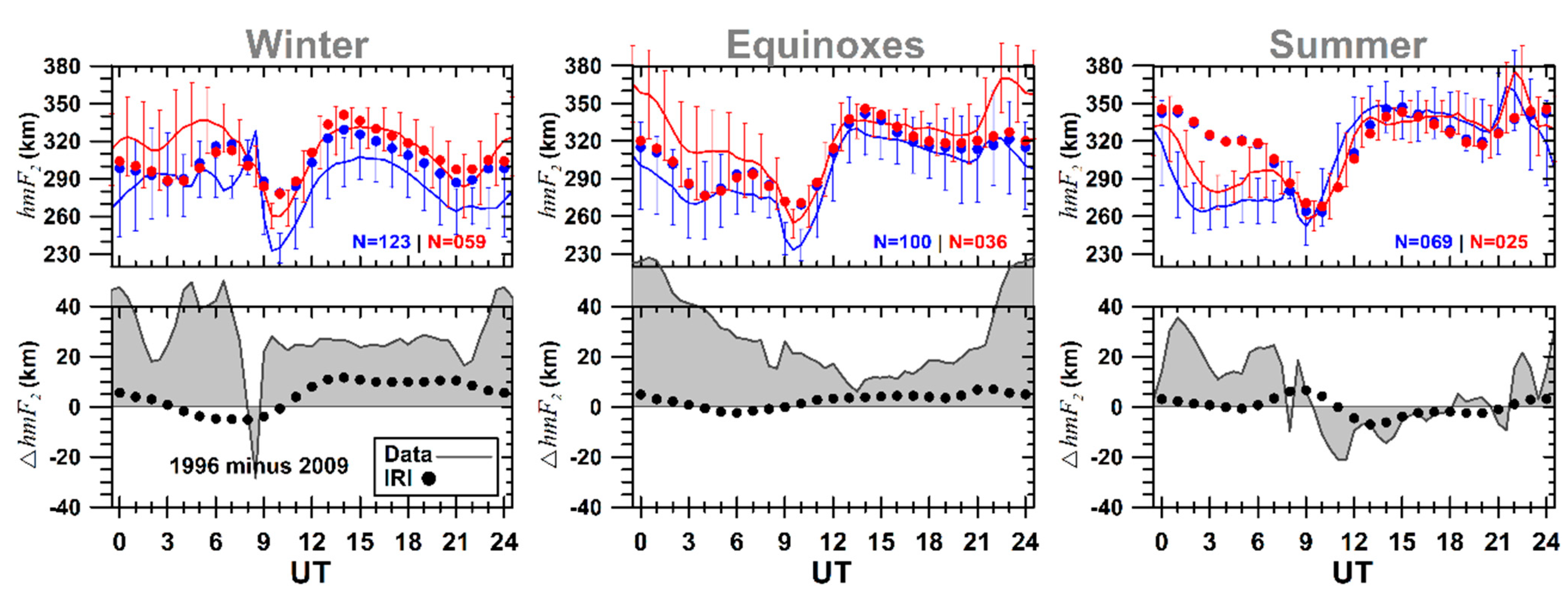
3.1. Dependence of the Model and the Observational F₂ Peak Parameters with Respect to Time and Season

The upper panels of Figure 3 and Figure 4 show the universal time (UT) and seasonal variability of the hmF₂ and foF₂, respectively, over São Luís during 1996 (red) and 2009 (blue) based on observational (solid curves) and modeled IRI data (dotted curves) (this work used the IRI 2016 version and the URSI coefficients to obtain the modeled F-layer peak parameters). The average values of foF₂ and hmF₂ and their respective standard deviation were calculated every 30 min in the case of observational data and at each hour in the case of the modeled data. The 122 days centered on 21 June (21 December) were considered for the winter (summer) seasons, and the two 61-day periods centered on 20 March and 23 September were considered to represent the equinox period, as mentioned before. The number of days used in the calculation is indicated in each panel by the N values. As mentioned previously, there is a lack of data from January to early March of 2009. Although the number of days used in calculating average values in 1996 is lower than in 2009, it is still considered statistically significant since they are reasonably spaced along the seasons. The bottom panels indicate the differences between the periods through the residual (indicated by Δ), which is the data or IRI predictions of 1996 minus 2009.

In general, the mean values of observed hmF₂ in 2009 were lower than in 1996, except in the summer when the hmF₂ during the deep solar minimum presented slightly higher values between 09:30 UT and 18:00 UT (Figure 3). These characteristics can be easily identified by the predominant positive values of ∆hmF₂ (lower panels) in the case of winter and equinoxes and negative values during the daytime in the summer. Additionally, it is possible to verify that the lowest difference between the observed data for 1996 and 2009 (gray area) occurred during the summer. Figure 3 also reveals that: (i) The F layer rise at sunset (~21:30–22:00 UT) due to the PRE in the equinoxes of 1996 was ~40 km higher than in 2009. In the summer, only 10 km of difference was observed. Besides that, the PRE was observed some minutes earlier in 2009 than in 1996, mainly during the equinoxes; (ii) The occurrence of the PRE during the winter seems to occur later in 1996 when compared to other seasons since in 2009 it seems to have absent; (iii) Regarding the performance of the IRI model (dotted curves), we may note that, in general, the model representation during the daytime was better than that of the nighttime for both periods, except in the winter of 2009, when the model prediction was higher than the observational data; (iv) Between 00:00 UT and 09:00 UT, the performance of the IRI was better in 2009 than in 1996 during the winter and equinoxes. At 04:00 UT, for example, while the hmF2 in 2009 simulated by the IRI was similar to the observed data for both seasons, in 1996, it was overestimated by the IRI for about 40 and 34 km in winter and equinoxes, respectively. During the summer, the model did not correctly reproduce both the 1996 and the 2009 data; (v) The comparison between the gray area and the black points in the lower panels indicates that, in general, the IRI model predicted the behavior of the F layer peak height during 2009 in a very similar way as that in 1996, a situation that does not correspond to what the observational data showed. Interestingly, the higher hmF₂ values in 2009 in the summer were predicted by the IRI as indicated by the negative black points in the lower panel of the summer block, but with a smaller amplitude when compared to the data.

Figure 4 shows a similar analysis to Figure 3, but now considering the foF₂ variation. Similar to what was observed for hmF₂, the seasonal dependence is very clear, and the value of foF₂ was higher in 1996 for all seasons studied, mainly during the nighttime period in summer. In general, better representation by the IRI model was observed during the daytime for winter and equinoxes, and once again for the summer, the model predicted higher values than the data for both years in this period. However, between 00:00 UT and 08:00 UT, better performance of the IRI was evident in the summer of 2009. Taking as reference the time at 02:00 UT, the values simulated by the IRI in 2009 (1996) were about 67% (56%) and 23% (13%) higher than the observational data during the winter and equinoxes, respectively. For the summer, the model IRI underestimated the data by 10% in 2009 and 15% in 1996. Regarding the ∆foF₂ (lower panels), it is possible to verify that the lowest difference between the observational data of 1996 and 2009 occurred in the winter. For the equinoxes and summer, the differences between daytime were equivalent, therefore, more significant in the summer between 02:00 UT and 08:00 UT. Similar to what was observed in the case of ∆hmF₂, the F₂ model of critical frequency in 2009 was very similar to 1996, not predicting in this way the real behavior of the ionosphere for both epochs.

3.2. Climatology of the Tidal Modes

To investigate the amplitude and the solar diurnal, semidiurnal, and terdiurnal periodicities of the F layer peak parameters, the Fast Fourier Transform analysis was applied to every day of data from 1996 to 2009 using the following equation:

$$\mathit{x}{\mathit{V}}_{\left(\mathit{t}\right)}=\mathit{A}\mathbf{0}+\mathbf{2}{\displaystyle \sum }_{\mathit{m}=\mathbf{1}}^{\mathbf{3}}\left[\mathit{A}{\mathit{m}}_{\left(\mathit{m}\right)}\mathbf{cos}\left(\mathbf{2}\mathit{\pi }\mathit{m}{\mathit{f}}_{\mathbf{1}}\mathit{t}\right)+\mathit{B}{\mathit{m}}_{\left(\mathit{m}\right)}\mathbf{sin}\left(\mathbf{2}\mathit{\pi }\mathit{m}{\mathit{f}}_{\mathbf{1}}\mathit{t}\right)\right]$$

(1)

where $x{V}_{\left(t\right)}$ is the reconstructed variable as a function of time in UT (t) ($xV$ stands for hmF₂ or foF₂), $f_1$ is the fundamental frequency of the parameter to be reconstructed (1/24), $A0$ is the daily average of such parameter for a given day of the year, and finally, $A{m}_{\left(m\right)}$ and $B{m}_{\left(m\right)}$ are the m^th Fourier coefficients also as a function of time (UT). The terms $A{m}_{\left(m\right)}$ and $B{m}_{\left(m\right)}$ together are the amplitudes for the harmonics m = 1 (24 h), m = 2 (12 h), and m = 3 (8 h).

Figure 5 shows the daily amplitude (A0), diurnal (m = 1), semidiurnal (m = 2), and terdiurnal (m = 3) components in respect of the day of the year (DOY) for the 1996 and 2009 periods (red and blue dots, respectively) for the foF₂ (left panels) and the hmF₂ (right panels). The continuous lines represent the best polynomial approximation to the data (the correlation coefficient—R—is also given for each one of the approximations). It can be noted that a good correlation was found between the data and polynomial fitting for both F₂ peak parameters for the amplitude, diurnal and semidiurnal mode (independently of the studied period). It can be noted that the R values for 2009 were higher than in 1996, except for the 12 h component of hmF₂. This better correlation in 2009 can be related to the quieter period of 2009, as revealed in Figure 2. The amplitude of foF₂ presented an annual and a semiannual component for both the studied periods, being clearly higher for 1996, mainly for the southern spring equinox (from the beginning of September to the end of November). For 26 October (DOY 301), where the difference between the two periods is more prominent, the amplitude of foF₂ was about 25% higher in 1996. For the amplitude of hmF₂, the higher difference was noted in mid-June (June solstice), when the hmF₂ amplitude in 1996 was higher than in 2009 by ~10%. The value of hmF2 presented an annual and semiannual component for 1996 and only an annual component for 2009. Additionally, it can be observed that for the diurnal (24 h) component, there is a similarity in the results for both height and frequency parameters, as can be seen by the solid blue and red curves. Nonetheless, some differences were found for semidiurnal and terdiurnal components. In these cases, the value for 2009 was generally lower than for 1996, except in some intervals. The significant contribution of the diurnal component to the variability of foF2 in the months that approaches the winter (with a peak in June) can be clearly noted. A similar trend is not seen in hmF₂, as the semidiurnal variability seems to be more important. It is interesting to observe the significant contribution of the 8 h tide to the foF2 variation, mainly in the winter months for both years, and to the hmF2 variation, especially from September to December of 2009.

The next step is verifying how realistic is the IRI model in representing the tidal components for these periods of solar minimum activity, especially in 2009. Figure 6 shows the same results as Figure 5 but now includes the results from the IRI model (crossed curves). For the foF₂ amplitude, it is possible to observe that, in general, the IRI model represented well the 1996 period during the first four months of the year; however, it overestimated the observational data for the period of mid-April (DOY 105) to the end of July (DOY 209). On the other hand, an underestimation in the last months of the year can be noted, with a maximum in November. In 2009, the model overestimated the amplitude of observational data during almost the period analyzed. Regarding the value of the height parameter, the representation of the IRI was very poor for both years. For the 24 h, 12 h, and 8 h components of the foF₂, it can be verified as a bad representation by the IRI model, except in some periods of both years. For the hmF₂, the best representation can be seen in the second half of the year for both 1996 and 2009 for the case of the diurnal component and in the first half of the year for the case of the terdiurnal component.

Table 1. Amplitude, diurnal, semidiurnal, and terdiurnal periodicity of hmF₂ and foF₂ of equatorial latitude for the ionosonde data and the IRI predictions.

1996 2009	foF2				hmF2
	Ionosonde		IRI		Ionosonde		IRI
	12 months	6 months	12 months	6 months	12 months	6 months	12 months	6 months
Amplitude	××	××	××	××	××	×	××
m = 1 (24 h)	××		××	××	××		××	××
m = 2 (12 h)	××		××	××	××		××	××
m = 3 (8 h)	××	××	××	××	××	××	××	××

summarizes the results presented in Figure 6, considering the general behavior and not the intensity of analyzed parameters. We can note that IRI predictions failed to represent a semiannual behavior of a diurnal and semidiurnal component in the case of foF₂ for 1996 and 2009 since such characteristics are not seen in the observational data. For the hmF₂, besides the model indicating a semiannual behavior in 24 h and 12 h components that do not exist in agreement with observational data, the IRI model does not represent the semiannual behavior for the amplitude of hmF₂ in 1996.

4. Discussion

This work aims to investigate the impacts of solar minimum activities in the Brazilian equatorial ionosphere during the solar cycles 22/23 (1996) and 23/24 (2009). For that, we used the hmF₂ and foF₂ data collected by a Digisonde installed at São Luis, situated close to the magnetic equator in Brazil, and compared the observational data with the prediction by the IRI model to verify how realistic this model represents the solar activity minimum conditions, especially that of 2009.

Solar and geomagnetic activity directly affects the Earth’s thermosphere and ionosphere. Due to the uniqueness of solar cycle 23/24, which presented an unusual behavior, being deeper, longer, and also geomagnetically quieter than the previous minima as shown in Figure 1 and Figure 2, several authors have devoted their time to investigating this particular period, then making comparative studies involving both observational and modeled data during the same periods analyzed here (1996 and 2009) or periods close to these (see for example [8,13,15,17,26]).

4.1. Influence of Solar Flux in the Equatorial Ionosphere

The results presented here clearly revealed the impacts of the decrease in the level of solar extreme ultraviolet radiation in 2009 (see Figure 1) in both the ionospheric parameters of the top frequency (foF₂) and the peak height (hmF₂) over the equatorial latitude. The seasonal mean values of Figure 3 and Figure 4 show not only a significant deviation between the observational data of 1996 and 2009 but also a considerable discrepancy between the observational and the modeled data for both periods in some intervals. The electron density, which is expressed here in terms of foF₂, was overall higher in 1996, and the differences between the two minima were more pronounced during the equinoxes and summer. Since the ionosphere is very sensitive to changes in its ionization sources, it is believed that the decrease in foF₂ in 2009 is directly related to the decrease in solar EUV radiation during this period. However, an interesting characteristic in our results is related to the ∆foF₂ values, which will be discussed as follows.

As shown in Figure 4, the differences between foF₂ (∆foF₂) in 1996 and 2009, on average varied by 0.37 ± 0.11 MHz in the June solstice, 0.64 ± 0.21 MHz in the equinoxes, and 0.70 ± 0.44 MHz in the summer. However, the corresponding EUV variation (∆EUV) for these seasons in the band of 26–34 nm varied by 2.13, 1.93, and 1.98 × 10⁹ photons cm⁻² s⁻¹, respectively. Therefore, the differences observed in the foF₂ were not totally corresponding to the ∆EUV, as the higher ∆foF₂ occurred in summer, while the higher ∆EUV was observed in the winter. This indicates that other processes also must be controlling the electron density (foF₂) variation in the equatorial latitude over São Luis. On the other hand, the differences observed in hmF₂ were higher in winter and equinoxes. During the summer, a curious behavior was observed in the height parameter during the daytime. In this case, a negative value of ∆hmF₂ was found, which means that the peak height of the F layer in 2009 was higher than in 1996 during a particular interval of the day. Excluding this specific period, the hmF₂ over São Luis was higher in 1996 than in 2009. Such a result is expected since the upper atmosphere and ion temperature became cooler during the deep solar minimum (see, for example, [10]). This cooling in the temperature can consistently explain the observed nature of equatorial hmF₂. According to [27], the larger temperature decrease due to the doubling of CO₂ under solar minimum conditions causes a larger decrease in plasma scale height.

Using ionosonde data over the equatorial site of Jicamarca during the solar minimum periods of 1996–1997 and 2008–2009, [9] reported that the higher ∆foF₂ (~2 MHz at nighttime) occurred in September equinox, that it was coincident with the higher ∆EUV for the corresponding period studied. In turn, [28] observed that the higher difference in foF₂ (1995 value minus 2009 value) occurred in March Equinox (~1.81 MHz) over the low latitude sector of India. For this season, they also verified higher ∆f_peak and ∆foF₃ values, which were 1.95 and 1.64 MHz, respectively.

Araujo-Pradere and collaborators [26] mentioned a complexity in the maximum electron concentration of the F region (NmF₂) over the midlatitudes regions (the NmF₂ parameter is directly related to the foF₂ through the expression NmF₂ [cm⁻³] = 1.24 × 10⁴ foF₂² [MHz] [13]. Although the authors observed a consistent depletion in the total ionospheric plasma content (vTEC) from the 22/23 minimum to the 23/24 minimum, a complex behavior was seen in the NmF₂ parameter. It was observed that the average value of this parameter in some cases was higher for the deep solar minimum than in the previous one and did not present a clear and consistent decrease as observed for the vTEC. The authors concluded that the mixed behavior in the vertical TEC and NmF₂ could indicate the depletion of the total ionospheric plasma content due to a decrease in the EUV ionization, while the ionization at the F-region peak may be associated with the movement of the plasma by the electric fields or neutral-wind interactions. This indicates that although less plasma was created during the 23/24 minimum, the global plasma dynamics played a very important role in the peak F-region electron density. The investigations of Liu and co-authors [9] also revealed that the ionosphere could respond in a complicated way to the reduction in solar input, as seen in the lower ∆N_e values that were not coincident with the lower ∆EUV.

The results presented in Figure 3 indicate that PRE probably occurred later in the winter when compared to other seasons in 1996 since, in 2009, the PRE seems to have been absent. During the equinoxes, the hmF₂ was expressively higher in 1996; however, the prereversal vertical drift (Vz) was slightly higher in 2009 (~4.00 m/s) than in 1996 (3.54 m/s). In the summer, a small difference in the Vz value between the two periods (being 6.57 m/s in 2009 and 6.78 m/s in 1996) was found. The Vz values mentioned above were calculated considering the time variability in the hmF₂, that is, ΔhmF₂/Δt. Over Jicamarca, the absence/presence of vertical drift in the winter/equinoxes was observed for both the solar minimum periods. Besides that, different from what was observed over Sao Luis, the PRE over the Peruvian sector was not identified during the summer in the 23/24 solar minimum [9]. Regarding the time of the PRE occurrence, it was noted that in 2009 it occurred a few minutes earlier than in 1996, mainly during the equinoxes. Such peculiarities seem to be typical of the Brazilian sector since a similar behavior was not observed in the equatorial region of Jicamarca. As the PRE is an important parameter for the development of the plasma bubbles (see, for example, [29]), our results indicate that the spread-F development in the equinoxes may have occurred earlier in the solar minimum of 2009 than in 1996. However, more precise investigations of this point need to be performed.

Rishbeth and Mendillo [30] mentioned that the modulation of solar EUV flux primarily drives the F-layer variability, but the geomagnetic activity and meteorological sources at lower levels in the atmosphere also play an important role. As shown in Figure 2, the geomagnetic activity in 2009 was lower than in 1996 [31], but still, it was strong enough to modify the ionospheric parameters. For example, Ref. [32] reported that even under weak geomagnetic activity, the daily mean global electron content (GEC) varied significantly on short-term time scales during the 2007–2009 deep solar minimum. They showed that daily mean GEC was positively correlated with geomagnetic activity, represented by the Ap index. On the other hand [33] showed that the foF₂ and hmF₂ at Jicamarca and the TEC in the equatorial ionization anomaly region over the American longitudinal sector could be affected by the high-speed solar wind stream during the occurrence of geomagnetic storm events during the solar minimum year 2008. Buresova and co-authors [34] also investigated the ionospheric response to occasional magnetic disturbances at the middle latitudes under the extremely low solar activity conditions of 2007–2009. They found characteristics similar to those observed during strong magnetic storms. In turn, Ref. [35] have shown that even a small variation in geomagnetic activity (represented by the Kp index) can impact the parameters of height and frequency of intermediate layers over the Brazilian low latitude region (Cachoeira Paulista, 22.42° S; 45° W) during the solar minimum period of 2009. During such a period, geomagnetic variations were present, as shown in Figure 2. Cai et al. (2021) [36], in turn, suggested the geomagnetic forcing as a plausible source of mid-latitude thermospheric composition and ionosphere density variations even during some “geomagnetically quiet” periods at solar minimum. They observed a day-to-day variability of ∼30% in the thermospheric composition and ionospheric total electron content under geomagnetically quiet conditions (Kp < 2). These results indicate that, although this period has been extremely calm, it is still sensitive to geomagnetic disturbances.

As mentioned previously, meteorological sources can also play an important role in ionospheric variability. During the data processing, strong modification in the F-layer trace was visually noted in 2009 that can be related to gravity wave propagation. Some examples can be found in Figure 13 of [37]. In agreement with these authors, large modifications in the F₁ and F₂ layers were noticed, in the form of bifurcations and forking traces in both F₁ and F₂ layers, besides other modifications that were not very well defined. For the same period [38] also showed an anomalous case in June 2009, in which the ionospheric F₂ layer trace over SL appeared to have “broken in half” making it appear that the first part of the F₂ layer (at the lower frequency region) was thrown down whilst the upper part of the trace remained at higher altitudes. In agreement with these papers, all of these features were attributed to a possible manifestation of gravity waves. Considering that the ionosphere was considerably contracted due to the extremely low level of solar fluxes, the tides and waves originating in the lower atmosphere can be expected to register their effects in the thermosphere and ionosphere more easily [2]. Although we have not quantified in our analysis the effects of magnetic and meteorological disturbances, we cannot neglect their possible impacts on the foF₂ and the hmF₂ parameters.

4.2. IRI-2016 Performance during Anomalous Solar Minimum

The results demonstrated in Figure 3 and Figure 4 indicated that, in general, the IRI modeled the behavior of the F₂ layer peak parameters in 2009 in a very similar to 1996, a condition that does not correspond to reality since the observational data during the deep solar minimum was lower than (excepted in some intervals) the data of the period that is considered as “normal” in terms of solar flux. However, it was interesting to observe what happened in the summer, when the slightly higher values of hmF₂ in 2009 in a specific interval of day-time were predicted by the IRI, although with a smaller amplitude when compared with the observational data. The impacts of solar atmospheric tides on our data were also investigated and compared with the IRI predictions. Such analysis is a novelty since we didn’t find something similar, at least on the references cited here. Atmospheric tides are defined as global scale oscillations that can be observed in all types of atmospheric fields, such as wind, temperature, pressure, and density, with periods that are subharmonics of a solar day [39]. They are primarily excited by the solar heating of atmospheric gases, including tropospheric water vapor, stratospheric and mesospheric ozone, and O₂ in the lower thermosphere [40]. Besides other meteorological influences, geomagnetic activity, solar flux, and atmospheric tides can also be considered important sources of ionospheric variability. Our results, for example, showed clearly the impacts of the tides on height and frequency parameters over the equatorial region both for 1996 and 2009, as shown in Figure 5 and Figure 6.

Regarding the different components of the tide, we highlight the similar results observed for 1996 and 2009 in the case of the diurnal component, the differences in the semidiurnal component in both the hmF₂ and the foF₂, and the impact of the terdiurnal component on the foF₂ and the hmF₂ variabilities. With respect to the last factor [41] mentioned that the 8 h tide variability in the ionosphere has attracted significant interest from the scientific community. For example, Gong and Zhou [42] reported the importance of the F region terdiurnal tide amplitude, which in general, is smaller than that of the diurnal tide. Such a result agrees with our results for foF₂, as seen in the left panel of Figure 6. Besides that, it can be observed that the foF₂ terdiunal component was higher than the semidiurnal tide until October (for both years). On the other hand, the hmF₂ terdiurnal amplitude can present the same amplitude or even be bigger than the diurnal component for the winter period. As shown in the right panels of Figure 6, the amplitude of the 8 h component was lower than the 24 h component during the summer and equinoxes (for both years); however, it was higher or compatible with the amplitude of the diurnal component in the winter. These results are evidence of the significant role of the terdiurnal tide in the hmF₂ variability

In relation to the prediction by the IRI model on the amplitude of the tidal components, a reasonable performance was observed in the case of foF₂. Although the intensity of the amplitude had not been correctly estimated (mainly for 2009), the model correctly predicted the semiannual behavior. In the case of the hmF₂, quite poor results with the IRI were found in both years. As shown in Figure 6, only a few cases/intervals of the model prediction were compatible with what was observed.

5. Final Remarks

Based on the ionograms recorded by a Digisonde operated at the equatorial site of São Luis, this work investigated the behavior of the foF₂ and the hmF₂ parameters during the solar cycles 22/23 (1996) and 23/24 (2009) by comparing the observational data with the IRI model. The main findings are summarized below:

• In general, the mean values of the hmF₂ and the foF₂ during the deep solar minimum were lower than in 1996, except in some intervals, such as in the summer, when the hmF₂ in 2009 presented slightly higher values in a specific interval of daytime when compared to 1996. Interestingly, such behavior was predicted by the IRI but with a smaller amplitude when compared with data;
• The seasonal mean values of the hmF₂ and the foF₂ presented significant deviations between their respective values for 2009 and 1996. The considerable discrepancy between the observation and the model was also observed during both years, except during some daytime intervals;
• During the equinoxes, the prereversal vertical drift (Vz) was slightly higher in 2009 (~4.00 m/s) than in 1996 (3.54 m/s). In the summer, a small difference in the Vz value for both periods (6.57 m/s in 2009 and 6.78 m/s in 1996) was found. Additionally, the PRE occurred in 2009 occurred some minutes earlier than in 1996, mainly during the equinoxes.
• The analysis of atmospheric tides showed some differences between the two minima for both amplitudes of hmF₂ and foF₂, which were higher in 1996 than in 2009 for almost all the days analyzed. Regarding the different tide components, the contribution of the diurnal component to the hmF₂ variability was similar in both periods. When compared to 12 h tide, the most important contribution of the semidiurnal tide was observed from April to September for both 1996 and 2009. It is also important to mention that the terdiurnal and the semidiurnal periodicities have similar annual amplitude, about 21 km (hmF₂) and 0.8 MHz (foF₂). However, the hmF₂ and foF₂ terdiurnal and the semidiurnal tide components present opposite behavior throughout the year; the terdiurnal hmF₂/foF₂ component is smaller/higher than the semidiurnal component during the winter and higher/smaller for the summer period.
• The amplitude of foF₂ was higher in 1996 than in 2009, mainly in the second half of the year. In general, the higher intensity of tide components was observed for 1996, except for the 24 h component, which presented similar results for both solar minimum periods. Additionally, besides the important contribution of the diurnal component in the foF₂ variability, the terdiurnal component in the foF₂ is also highlighted when compared with the semidiurnal component, which has been higher than the semidiurnal tide for almost the whole year, except for the southern summer.
• In the case of the foF₂ amplitude, a good representation by the IRI model was observed during the first four months of 1996; however, an overestimation was observed in the mid of April to the end of July. On the other hand, an underestimation was noted in the last months of the year, with a maximum in November. In 2009, the model overestimated the observational data during almost the period analyzed. For the 24 h, 12 h, and 8 h components, the representation by the IRI model was not good for both years, except in some cases.
• In the case of the hmF₂ amplitude, the prediction made by the IRI was very poor for both years. The best representation of the diurnal component was found in the second half of the year during both 1996 and 2009. In the case of the terdiurnal component, the best representation was found during the first half of the year. Finally, the importance of the terdiurnal component to hmF₂ and foF₂ variability was not predicted by the IRI, which is different from what was observed in the observational data.
• Finally, our results clearly showed the impacts of a decrease in the level of solar extreme ultraviolet radiation in 2009 on both the ionospheric parameters of frequency and height. However, it was also shown that such a decrease alone could not totally explain all the observed features. Additionally, similar to what has been reported by other authors, the model IRI needs some improvements to better represents the solar minimum periods.

References

1. Basu, S. The peculiar solar cycle 24—Where do we stand? J. Phys. Conf. Ser. 2013, 440, 012001. [Google Scholar] [CrossRef] [Green Version]
2. Balan, N.; Chen, C.Y.; Rajesh, P.K.; Liu, J.Y.; Bailey, G.J. Modeling and observations of the low latitude ionosphere plasmasphere system at long deep solar minimum. J. Geophys. Res. 2012, 117, A08316. [Google Scholar] [CrossRef]
3. Kutiev, I.; Tsagouri, I.; Perrone, L.; Pancheva, D.; Mukhtarov, P.; Mikhailov, A.; Lastovicka, J.; Jakowski, N.; Buresova, D.; Blanch, E.; et al. Solar activity impact on the Earth’s upper atmosphere. J. Space Weather Space Clim. 2013, 3, A06. [Google Scholar] [CrossRef] [Green Version]
4. Solomon, S.C.; Woods, T.N.; Didkovsky, L.V.; Emmert, J.T.; Qian, L. Anomalously low solar extreme-ultraviolet irradiance and thermospheric density during solar minimum. Geophys. Res. Lett. 2010, 37, L16103. [Google Scholar] [CrossRef]
5. Mansoori, A.A.; Khan, P.A.; Ahmad, R.; Atulkar, R.; Aslam, A.M.; Bhardwaj, S.; Malvi, B.; Purohit, P.K.; Gwal, A.K. Evaluation of long term solar activity effects on GPS derived TEC. J. Phys. Conf. Ser. 2016, 759, 012069. [Google Scholar] [CrossRef] [Green Version]
6. Araujo-Pradere, E.A.; Fuller-Rowell, T.J.; Codrescu, M.V. Storm: An empirical storm-time ionospheric correction model—1. Model description. Radio Sci. 2002, 37, 1–12. [Google Scholar] [CrossRef] [Green Version]
7. Moses, M.; Panda, S.K.; Dodo, J.D.; Ojigi, L.M.; Lawal, K. Assessment of long-term impact of solar activity on the ionosphere over an African equatorial GNSS station. Earth Sci. Inf. 2022, 15, 2109–2117. [Google Scholar] [CrossRef]
8. Liu, L.; Chen, Y.; Le, H.; Kurkin, V.I.; Polekh, N.M.; Lee, C.-C. The ionosphere under extremely prolonged low solar activity. J. Geophys. Res. 2011, 116, A04320. [Google Scholar] [CrossRef] [Green Version]
9. Liu, L.; Yang, J.; Le, H.; Chen, Y.; Wan, W.; Lee, C.-C. Comparative study of the equatorial ionosphere over Jicamarca during recent two solar minima. J. Geophys. Res. 2012, 117, A01315. [Google Scholar] [CrossRef] [Green Version]
10. Heelis, R.A.; Coley, W.R.; Burrell, A.G.; Hairston, M.R.; Earle, G.D.; Perdue, M.D.; Power, R.A.; Harmon, L.L.; Holt, B.J.; Lippincott, C.R. Behavior of the O+/H+ transition height during the extreme solar minimum of 2008. Geophys. Res. Lett. 2009, 36, L00C03. [Google Scholar] [CrossRef]
11. Aponte, N.; Brum, C.G.M.; Sulzer, M.P.; González, S.A. Measurements of the O+ to H+ transition height and ion temperatures in the lower topside ionosphere over Arecibo for equinox conditions during the 2008–2009 extreme solar minimum. J. Geophys. Res. Space Phys. 2013, 118, 4465–4470. [Google Scholar] [CrossRef]
12. Coley, W.R.; Heelis, R.A.; Hairston, M.R.; Earle, G.D.; Perdue, M.D.; Power, R.A.; Harmon, L.L.; Holt, B.J.; Lippincott, C.R. Ion temperature and density relationships measured by CINDI from the C/NOFS spacecraft during solar minimum. J. Geophys. Res. 2010, 115, A02313. [Google Scholar] [CrossRef] [Green Version]
13. Brum, C.G.M.; Rodrigues, F.S.; dos Santos, P.T.; Matta, A.C.; Aponte, N.; Gonzalez, S.A.; Robles, E. A modeling study of foF2 and hmF2 parameters measured by the Arecibo incoherent scatter radar and comparison with IRI model predictions for solar cycles 21, 22, and 23. J. Geophys. Res. 2011, 116, A03324. [Google Scholar] [CrossRef]
14. Klenzing, J.; Simões, F.; Ivanov, S.; Heelis, R.A.; Bilitza, D.; Pfaff, R.; Rowland, D. Topside equatorial ionospheric density and composition during and after extreme solar minimum. J. Geophys. Res. 2011, 116, A12330. [Google Scholar] [CrossRef]
15. Abdu, M.A.; CBrum, G.M.; Batista, I.S.; Sobral, J.H.A.; de Paula, E.R.; Souza, J.R. Solar flux effects on equatorial ionization anomaly and total electron content over Brazil: Observational results versus IRI representations. Adv. Space Res. 2008, 42, 617–625. [Google Scholar] [CrossRef]
16. Souza, J.R.; Brum, C.G.M.; Abdu, M.A.; Batista, I.S.; Asevedo, W.D.; Bailey, G.J.; Bittencourt, J.A. Parameterized Regional Ionospheric Model and a comparison of its results with experimental data and IRI representations. Adv. Space Res. 2010, 46, 1032–1038. [Google Scholar] [CrossRef]
17. Batista, I.S.; Abdu, M.A. Ionospheric variability at Brazilian low and equatorial latitudes: Comparison between observations and IRI model. Adv. Space Res. 2004, 34, 1894–1900. [Google Scholar] [CrossRef]
18. Rush, C.; Fox, M.; Bilitza, D.; Davies, K.; McNamara, L.; Stewart, F.; PoKempner, M. Ionospheric mapping—An update of foF2 coefficients. Telecomm. J. 1989, 56, 179–182. [Google Scholar]
19. Altadill, D.; Magdaleno, S.; Torta, J.M.; Blanch, E. Global empirical models of the density peak height and of the equivalent scale height for quiet conditions. Adv. Space Res. 2013, 52, 1756–1769. [Google Scholar] [CrossRef]
20. Bilitza, D. The International Reference Ionosphere—Status 2013. Adv. Space Res. 2015, 55, 1914–1927. [Google Scholar] [CrossRef]
21. Bilitza, D. IRI the International Standard for the Ionosphere. Adv. Radio Sci. 2018, 16, 1–11. [Google Scholar] [CrossRef]
22. Brown, S.; Bilitza, D.; Yiğit, E. Ionosonde-based indices for improved representation of solar cycle variation in the International Reference Ionosphere model. J. Atmos. Sol.-Terr. Phys. 2018, 171, 137–146. [Google Scholar] [CrossRef]
23. Bilitza, D.; Pezzopane, M.; Truhlik, V.; Altadill, D.; Reinisch, B.W.; Pignalberi, A. The International Reference Ionosphere model: A review and description of an ionospheric benchmark. Rev. Geophys. 2022, 60, e2022RG000792. [Google Scholar] [CrossRef]
24. Terra, P.; Vargas, F.; Brum, C.G.M.; Miller, E.S. Geomagnetic and solar dependency of MSTIDs occurrence rate: A climatology based on airglow observations from the Arecibo Observatory ROF. J. Geophys. Res. Space Phys. 2020, 125, e2019JA027770. [Google Scholar] [CrossRef]
25. Matzka, J.; Stolle, C.; Yamazaki, Y.; Bronkalla, O.; Morschhauser, A. The geomagnetic Kp index and derived indices of geomagnetic activity. Space Weather 2021, 19, e2020SW002641. [Google Scholar] [CrossRef]
26. Araujo-Pradere, E.A.; Redmon, R.; Fedrizzi, M.; Viereck, R.; Fuller-Rowell, T.J. Some Characteristics of the Ionospheric Behavior During the Solar Cycle 23–24 Minimum. Sol. Phys. 2011, 274, 439–456. [Google Scholar] [CrossRef]
27. Qian, L.; Solomon, S.C.; Roble, R.G.; Kane, T.J. Model simulations of global change in the ionosphere. Geophys. Res. Lett. 2008, 35, L07811. [Google Scholar] [CrossRef] [Green Version]
28. Chaitanya, P.P.; Patra, A.K.; Balan, N.; Rao, S.V.B. Unusual behavior of the low-latitude ionosphere in the Indian sector during the deep solar minimum in 2009. J. Geophys. Res. Space Phys. 2016, 121, 6830–6843. [Google Scholar] [CrossRef]
29. Abdu, M.A. Equatorial spread F development and quiet time variability under solar minimum conditions. Indian J. Radio Space Phys. 2012, 42, 168–183. [Google Scholar]
30. Rishbeth, H.; Mendillo, M. Patterns of F2-layer variability. J. Atmos. Sol.-Terr. Phys. 2001, 63, 1661–1680. [Google Scholar] [CrossRef]
31. Kilpua, E.K.J.; Luhmann, J.G.; Jian, L.K.; Russell, C.T.; Li, Y. Why have geomagnetic storms been so weak during the recent solar minimum and the rising phase of cycle 24? J. Atmos. Sol.-Terr. Phys. 2014, 107, 12–19. [Google Scholar] [CrossRef]
32. Chen, Y.; Liu, L.; Le, H.; Wan, W. Geomagnetic activity effect on the global ionosphere during the 2007–2009 deep solar minimum. J. Geophys. Res. Space Phys. 2014, 119, 3747–3754. [Google Scholar] [CrossRef]
33. Liu, J.; Liu, L.; Zhao, B.; Wei, Y.; Hu, L.; Xiong, B. High-speed stream impacts on the equatorial ionization anomaly region during the deep solar minimum year 2008. J. Geophys. Res. 2012, 117, A10304. [Google Scholar] [CrossRef] [Green Version]
34. Buresova, D.; Lastovicka, J.; Hejda, P.; Bochnicek, J. Ionospheric disturbances under low solar activity conditions. Adv. Space Res. 2014, 54, 185–196. [Google Scholar] [CrossRef]
35. Santos, Â.M.; Brum, C.G.M.; Batista, I.S.; Sobral, J.H.A.; Abdu, M.A.; Souza, J.R. Responses of intermediate layers to geomagnetic activity during the 2009 deep solar minimum over the Brazilian low-latitude sector. Ann. Geophys. 2022, 40, 259–269. [Google Scholar] [CrossRef]
36. Cai, X.; Burns, A.G.; Wang, W.; Qian, L.; Pedatella, N.; Coster, A.; Zhang, S.; Solomon, S.C.; Eastes, R.W.; Daniell, R.E. Variations in thermosphere composition and ionosphere total electron content under “geomagnetically quiet” conditions at solar-minimum. Geophys. Res. Lett. 2021, 48, e2021GL093300. [Google Scholar] [CrossRef]
37. Dos Santos, Â.M.; Batista, I.S.; Abdu, M.A.; Sobral, J.H.A.; de Souza, J.R.; Brum, C.G.M. Climatology of intermediate descending layers (or 150 km echoes) over the equatorial and low-latitude regions of Brazil during the deep solar minimum of 2009. Ann. Geophys. 2019, 37, 1005–1024. [Google Scholar] [CrossRef] [Green Version]
38. Santos, A.M.; Brum, C.G.M.; Batista, I.S.; Sobral, J.H.A.; Abdu, M.A.; Souza, J.R.; Chen, S.S.; Denardini, C.M.; de Jesus, R.; Venkatesh, K.; et al. Anomalous responses of the F2 layer over the Brazilian equatorial sector during a counter electrojet event: A case study. J. Geophys.Res. Space Phys. 2022, 127, e2022JA030584. [Google Scholar] [CrossRef]
39. Pancheva, D.; Miyoshi, Y.; Mukhtarov, P.; Jin, H.; Shinagawa, H.; Fujiwara, H. Global response of the ionosphere to atmospheric tides forced from below: Comparison between COSMIC measurements and simulations by atmosphere-ionosphere coupled model GAIA. J. Geophys. Res. 2012, 117, A07319. [Google Scholar] [CrossRef]
40. Chang, J.L.; Avery, S.K. Observations of the diurnal tide in the mesosphere and lower thermosphere over Christmas Island. J. Geophys. Res. 1997, 102, 1895–1907. [Google Scholar] [CrossRef]
41. Liu, J.; Wang, W.; Zhang, X. The characteristics of terdiurnal tides in the ionosphere. Astrophys. Space Sci. 2020, 365, 155. [Google Scholar] [CrossRef]
42. Gong, Y.; Zhou, Q. Incoherent scatter radar study of the terdiurnal tide in the E- and F-region heights at Arecibo. Geophys. Res. Lett. 2011, 38, L15101. [Google Scholar] [CrossRef]
Figure 1. Solar activity representation based on the decimetric solar flux (F10.7 cm) (panel (a)) and the 26–34 nm and 0.1–50 nm EUV bands data measured by the Solar EUV Monitor onboard the Solar Heliospheric Observatory (SOHO) (panel (b)). Panel (c) shows the linear regression fitting over the two SOHO bands with respect to F10.7 cm. The red and blue colors represent the 1996 and 2009 solar minimums, respectively.
Atmosphere 14 00087 g001
Figure 2. Geomagnetic conditions of the periods in the study. Panel (a) shows the occurrence rate (in hours) of the Kp levels found in our data and those reported by [25]. Panel (b1) are the Kp daily sum but is distributed along the year (day of the year—DOY), while panel (b2) presents the 1996 minus 2009 Kp daily sum (the magenta dots denotes the monthly average, and the error bars indicate a 1 SD confidence interval).
Atmosphere 14 00087 g002
Figure 3. The universal time and seasonal variations of the hmF2 parameter over São Luís for 1996 (red) and 2009 (blue). The dots represent the IRI estimations (one-hour step), while the continuous lines are the 30 min averaged data by season (the error bars represent a 1 SD confidence interval for each 60-min). The N denotes the number of available days used for the average computation. The lower panels show the differences between 1996 and 2009 for the data (the gray area) and model (back points) for both periods (see text for more details). The local time (LT) for São Luis is related to the universal time as LT = UT − 3 h.
Atmosphere 14 00087 g003
Figure 4. Similar to Figure 3, but for foF2.
Atmosphere 14 00087 g004
Figure 5. Variability of the amplitude, diurnal (m = 1; 24 h), semidiurnal (m = 2; 12 h), and terdiurnal components (m = 3; 8 h) (from top to bottom) of the foF2 and the hmF2 parameters (left and right columns, respectively). The dots are the data, while the continuous lines represent the sixth-order polynomial approximation of them. The correlation coefficient R between the data and polynomial fitting is also shown. Red and blue for 1996 and 2009, respectively.
Atmosphere 14 00087 g005
Figure 6. Variability of the amplitude, diurnal, semidiurnal, and terdiurnal components of the best polynomial fitting of Figure 5 (continuous lines) and the parameters from IRI after applying the same methodology to which the data were submitted (crosses). Red and blue for 1996 and 2009, respectively.
Atmosphere 14 00087 g006