1. Introduction
The mathematical systematization of sports performance and talent search as a crucial mechanism for obtaining good players for large professional teams is known in both sports science and in the literature on sports management [
1]. In European and American contexts, the sports industry has a longer tradition in collecting statistical data, such as for baseball, soccer and basketball [
2,
3]. In recent years, digital economy has brought new technologies (player analysis) that have offered additional advantages, such as predicting player pairings or an athlete’s performance under specific conditions, all these based on classical statistical tools.
However, several sports organizations traditionally rely almost exclusively on the human experience for the talent process, even though in the past decades statistical computations were more heavily used [
4]. In soccer, it is still believed that experts in the field, such as coaches, managers and talent scouts, can effectively convert collected data into usable knowledge. For example, Louzada et al. [
5] proposed the creation of performance indicators based on multivariate statistical analysis. From this tool, one can quantify the performance of young players and take into account expert opinion for talent search or personalized training.
In this direction, Bayesian methods make it possible to combine the information contained in the observed data and the subjectivity of different experts in sports [
6]. The knowledge acquired from the experts will be added as a prior probabilistic distribution as, for example, these elements may consider aspects such as the expected recruitment of a player (to a certain team) or his/her physical performance.
The soccer national leagues, seen from a global perspective, generates results on a daily basis, which makes the amount of data that can be studied increase [
7]. That passion, which has various economic and social implications, is of great interest in order to see the linking of probabilistic models for the quantification of their results (and performance measurement). In this sense, statistical modeling applied to sports is a popular tool that has promoted various investigations [
8,
9,
10]. Two of the main aspects to investigate in the world of soccer are who will be the winner of the match? Or what will the number of goals scored by each team be? There have been various methodologies and probabilistic distributions used to carry this goal out, for example, in different studies the Binomial, Negative Binomial and Poisson distributions have been used, in addition to using both the classical and Bayesian inference perspectives.
Moreover, the Poisson distribution has been widely accepted as a suitable model for this kind of prediction; in particular, this model is often used because independence is assumed between the goals scored by the home team and the visitor (given its simplicity, which demands the estimation of a single parameter). For example, a soccer match can be seen as two models (), in which is the number of goals scored by the home team and is the number of goals scored by the visitor, though adopting the independence of the bivariate Poisson in which the relevant parameters are constructed as the combination of the attack and the defense of the teams.
For instance, Santana et al. [
11] adopted the Poisson distribution to estimate the probability of the vector (victory, tie, defeat) of each team on a given match. They demonstrated the effectiveness of this proposed model whereas a modified model (Poisson autoregressive model with exogenous covariates) was used to estimate the result of a given match, compared to previously adopted multinomial logistic regression and support vector machines models, which do not inform the score of the match (and the discrete probability model does).
In statistical methodology, Bayesian methods allow the inclusion of information from an investigator’s preliminary tests, allowing combination with the observed data. For instance, linear models can be understood as a combination of observed variables and latent effects, which can show hidden patterns, and can be adopted as a hierarchical Bayesian model to enable the estimation of individual effects in groups.
The present study proposed to develop a hierarchical Bayesian model to estimate the positions of the teams in the general table of the Chilean League 2020, saving the last five rounds as a prediction. The adopted model was based on the number of goals of each team to measure the attack power and defense both at home and away, and also the effect of home advantage. Hierarchical models are widely used as they are a natural way of taking into account the relationships between variables, assuming a common distribution for a set of relevant parameters that are believed to be related to one another.
The structure of this article is as follows:
Section 2 provides the basis for the model proposal,
Section 3 describes the proposed model and how the data were manipulated,
Section 4 describes the results in terms of parameter estimation and prediction of a new outcome, and finally
Section 5 highlights the respective conclusions and possible improvements to be made to following investigations.
2. Theoretical Framework
The sports world has always been interested in having a certainty of winning, since private teams invest large amounts of money to achieve good results. There are many aspects that are covered in the context of sports, such as the physical condition of the athletes, the maintenance of the place where the sport is developed, as well as having the best technical staff. This investment should ensure that it returns monetary gains.
A particular case is soccer tournaments, in which it seems difficult to predict the outcome of a game or who will be the winner in a certain championship, because there are many factors involved, such as those previously exposed (athletes, fields and technical personnel) as well as the presence of the public on the fields, injuries of the players, among others. Various studies have been able to predict winners of tournaments and matches, with different statistical models [
10,
12,
13]. An example of this is the large betting houses that, despite their work being based on “chance”, use models to benefit themselves and not the user.
Since the beginning of the 20th century, much data have been collected and, currently, the amount of data that can be collected is much higher, due to current technology. There have been several investigations into whether the result of soccer is luck or can be predicted [
7].
In this sense, seeking to model a soccer game, a game can be represented with the number of goals of the
gth team as a combination of the home versus away teams as
and
, respectively, in which the observed elements (the amount of goals) are bivariate variables
that can be modeled as independent events. Moreover, in a championship, the league is structured in such a way that every team will confront each other twice, once as the home team and another as the away team. In this case, the random variable that counts the number of goals is discrete, therefore the Poisson distribution would naturally be adopted as:
conditioned to the parameters
, which represent the play intensity of the home team (
i) and visitor team (
j), respectively.
For instance, let us consider a univariate discrete random variable
Y that follows a Poisson distribution [
14] with parameter
, represented by
, with probability mass function given by:
which has the property that the expectation and the variance are equal, that is,
.
Extending this univariate parameterization as a regression structure that associates explanatory factors to the composition of the parameter
, taking
a vector of independent variables, we have that a regression model could be written as
, in which
denotes a vector of regression coefficients. Thus, the extension of this statistical model, incorporating an explanatory vector structure (
) to estimate the parameter
, is:
If a bivariate discrete variable is considered, (), with independence, then each of the variables following a Poisson distribution are seen as . Additionally, if a Bayesian approach is adopted, the parameters are random variables, and one can estimate this regression model parameters, , as random variables effect (of each gth team) and assuming a log-linear as the (canonical) link function as:
MODEL 1 (NON-HIERARCHICAL):
The parameter represents the home advantage for the game taking place at home, which is assumed as constant for each team and match. The parameters and represent the ability to attack, and and the defense of each team. The elements considered indicate the n teams which are playing in the league.
Thus, for each of the parameters (
) indicated in the first modeling approach, which will enable us to estimate a common attack and defense structure among the teams in a championship, varying the scale parameters, however, also represent the league’s characteristics [
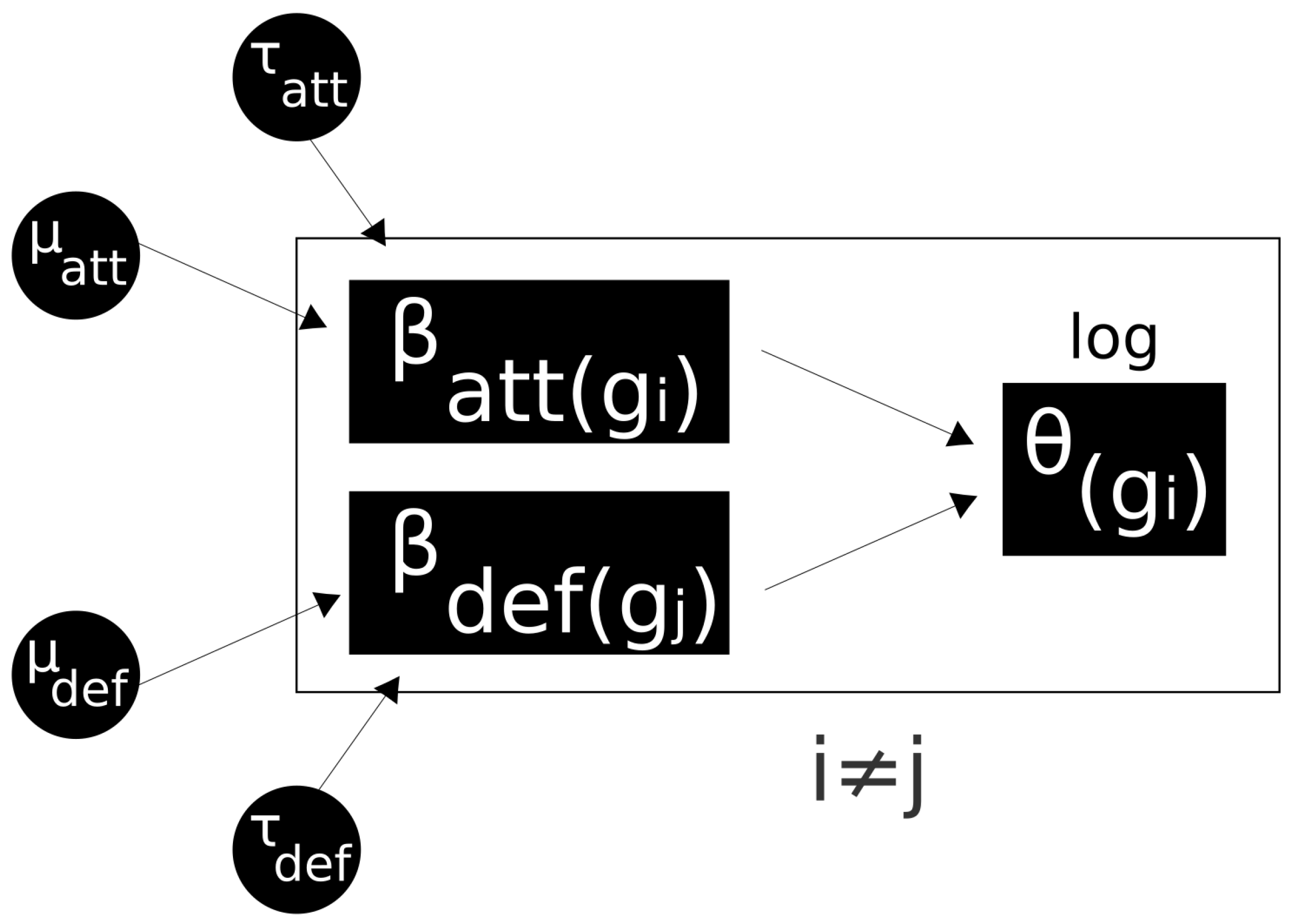
15]. Nevertheless, a second modeling approach is to consider the common shared structure added by a hierarchical level, which can design the attack strength of each team (regardless of playing at home or away), as well as the defense strength. Moreover, in the second model, the parameters (
and
) are centered though carrying hierarchical levels per team. For instance, the attack of each
gth team,
and
, can be seen as a random variable distributed with mean
and precision
.
MODEL 2 (HIERARCHICAL-Two levels):
The Bayesian modeling technique naturally adopts a hierarchical structure, enabling us to add levels to the structure that estimate each group’s influence (marginal) and their combination (global), that is, it also enables us to explain the common structure among those groups. These hierarchical models make it possible, in a natural way, to treat the levels’ data, avoid overfitting, and easily combine with custom decision analysis tools [
16].
Figure 1 summarizes the relationships between these parameters, and the statistical structure adopted to estimate the expected number of goals for each match.
The term hierarchical model is addressed by models with two or more levels in their random variable (as a single contribution). Additionally, it also assumes that all abilities (attacks and defenses) are derived from a common structure (league), or are mostly very similar. Through the Bayesian approach, the experts’ understandings are used as a priori information (although not a trivial task).
Hamiltonian Monte Carlo (Hmc) with Rstan
Under the Bayesian paradigm, statistical models can be calculated analytically from their posterior distributions, with reference to their parameters. However, deterministic integration methods are usually used to approximate these posterior distributions, which present a high complexity, especially under the presence of high dimensions.
Any unknown parameter (
) is associated with a probability function (
), which can be determined by Bayes’ theorem:
The first study that proposed a numerical approach for the posterior distribution
relating this integration problem and using the simulation based on states of molecule systems as a solution, was proposed by Metropolis [
17] and its updates are made via random walk. This technique is known as Markov chain Monte Carlo (MCMC). Consider a large independent and identically distributed sample (
), in which
, the posterior distribution will be the result of any function
g, via the law of large numbers:
Later, combining the idea of numerical approximation of the posterior distribution via resampling, Alder and Wainwright [
18] presented an alternative to the random walk following Newton’s laws of motion as Hamiltonian dynamics, which improved the estimation of the states, originating the Monte Carlo hybrid method or the Hamiltonian Monte Carlo (HMC). In order to search for the position of the variables and obtain inferences towards
, the method adds an auxiliary variable (
) called “momentum”. Therefore, the parameter space is explored through partial derivatives of the Hamilton’s equation converging much faster. For further investigation, please consult Brooks et al. [
19].
For Bayesian analysis, we used the integration of the programs R and Stan using the Shinystan package in R, which offers a variety of graphs and metrics tools, related to the convergence of the Monte Carlo chains, such as: , mcse/sd, HMC/NUTS and autocorrelation of each of the parameters, detailed by chain.
The metric
is composed by the total sample
N and the effective sample size
, in which the latter is calculated as:
with
n being the total sample size and
is the lag
k autocorrelation of parameters (
’s) (for further information, see [
19]). The
indicates the proportion of the parameters whose samples have effective size less than a certain percentage with respect to the total sample (regardless some significance level,
). It is also analyzed as each percentage of effective size impacting in each parameter.
We can also find the metric
mcse/sd, in which
mcse is the Monte Carlo standard error, which is the application of the delta method to the Monte Carlo estimates of the posterior variance [
19], and
sd is the standard deviation of the parameter’s posterior. Thus,
mcse/sd indicates the proportion of parameters whose standard errors are greater than a certain percentage with respect to the Monte Carlo estimates of the posterior variance [
20].
Another common metric is the
HMC/NUTS, in which
HMC represents the Hamiltonian Monte Carlo, which is an MCMC method that uses the derivatives of the density function of the sample to generate efficient procedures for the parameter’s posterior [
20]; and
NUTS (No-U-Turn Sampler) automatically selects an
(number of jump steps performed during Hamiltonian simulation) at each iteration to run posteriorly without doing unnecessary work. The idea is to avoid the random walk behavior that arises in the Metropolis or Gibbs samplers when there is correlation in the posterior distribution [
20].
From these metrics, the
Shinystan package [
21] generates a table considering each chain separately and together, in which, for the
HMC/NUTS, it shows the mean, standard deviation, maximum and minimum of the following properties of the chains:
accept_stat: For the HMC without NUTS, it is the Metropolis’ standard acceptance probability. A value closer to one is better (robust);
stepsize: The integrator used in the Hamiltonian simulation. If the value is large, it will be imprecise and reject too many proposals; and if it is small, it will take too many small steps, which will cause long simulation times per interval;
treedepth: A means that the first jump step is immediately rejected and returns to the initial state;
n_leapfrog: The number of jump steps performed during the Hamiltonian simulation. If its value is small, the sample will become a random walk; and if it is large, the algorithm will work more in each iteration;
divergent: The number of jump transitions with divergent error. This number is the average of divergence at each iteration;
energy: The Hamiltonian value in each sample. The energy diagnostic for HMC quantifies whether the tails of the posterior distribution are heavy or not.
4. Results
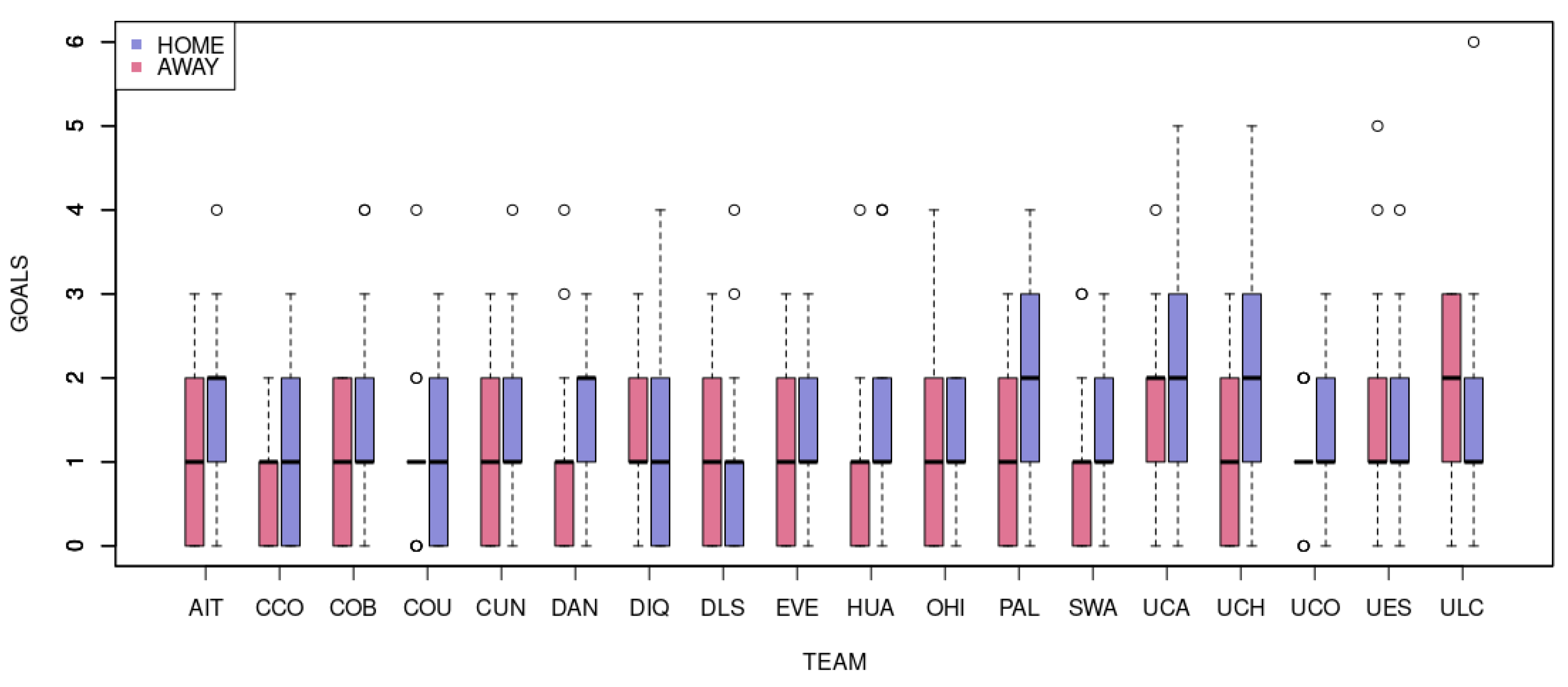
The 2020 Chilean First Division league is made up of 18 teams, which play against each other twice in a season (one at home and one away). This study took out the 34 rounds that occurred from 24 January 2020 to 17 February 2021, and the last five games were saved for validation. In the last rounds, 314 games were played, and the summarization of the scored goals through this championship is described, per team, in
Figure 2.
Considering the theoretical model of Poisson regression, we take as the response variable the number of goals scored by each team, explained by a home game factor added to their attack power and defense. The Shinystan package containing graphical and numerical summaries of parameters was adopted for the model and convergence diagnostics, and implemented in the R software for the analysis of the parameters with the HMC algorithm of strings with the size being 2000 iterations, with warmup = 1000 and thin = 1, with four independent chains. All statistical analyses of this study consider a credibility level of 50% (as statistical significance).
Both theoretical models, presented in
Section 2, were implemented and adopted the leave-one-out (LOO) cross-validation with moment matching aiming the model selection. The
loo package was adopted, based on the generated quantities from the STAN codes [
23].
Table 1 shows that the
loo results across the models are similar, and using the loo model comparison (function
loo_compare), the expected log pointwise predictive density (
elpd) difference between model 1 versus model 2 was −0.1 with a standard error (SE) of 0.6 (not differing statistically). Therefore, we chose model 2 because it contains fewer parameters.
In
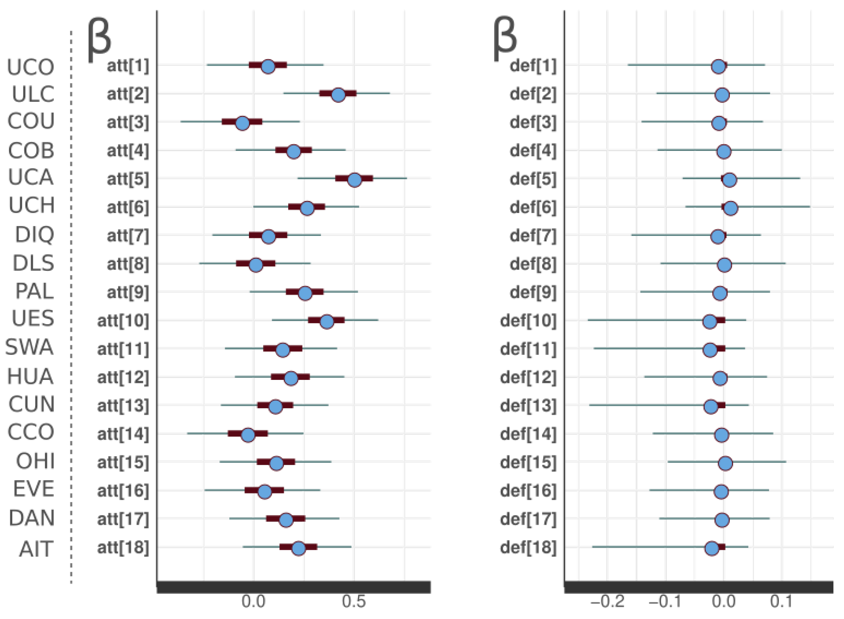
Table 2, we see, in detail, the descriptive statistics of the posterior distributions of the parameters of model 2 (hierarchical), which describe the expected scoring of the teams resulting in the final positions for the championship of 2020 (in which the last rounds will serve as a comparison and were not considered in the estimation process). It is possible to observe that the expected results of the three teams with the greatest attack power, foreseen by the adopted model, are in the first four positions of the final result table of the championship. Due to the model adopted, they are in the first four positions of the final result table of the championship. It should be noted that it was expected by the model that the other team in the top four is the Universidad de Chile (UCH), which we can place as having the fourth best attacking position in the graph of
Figure 3.
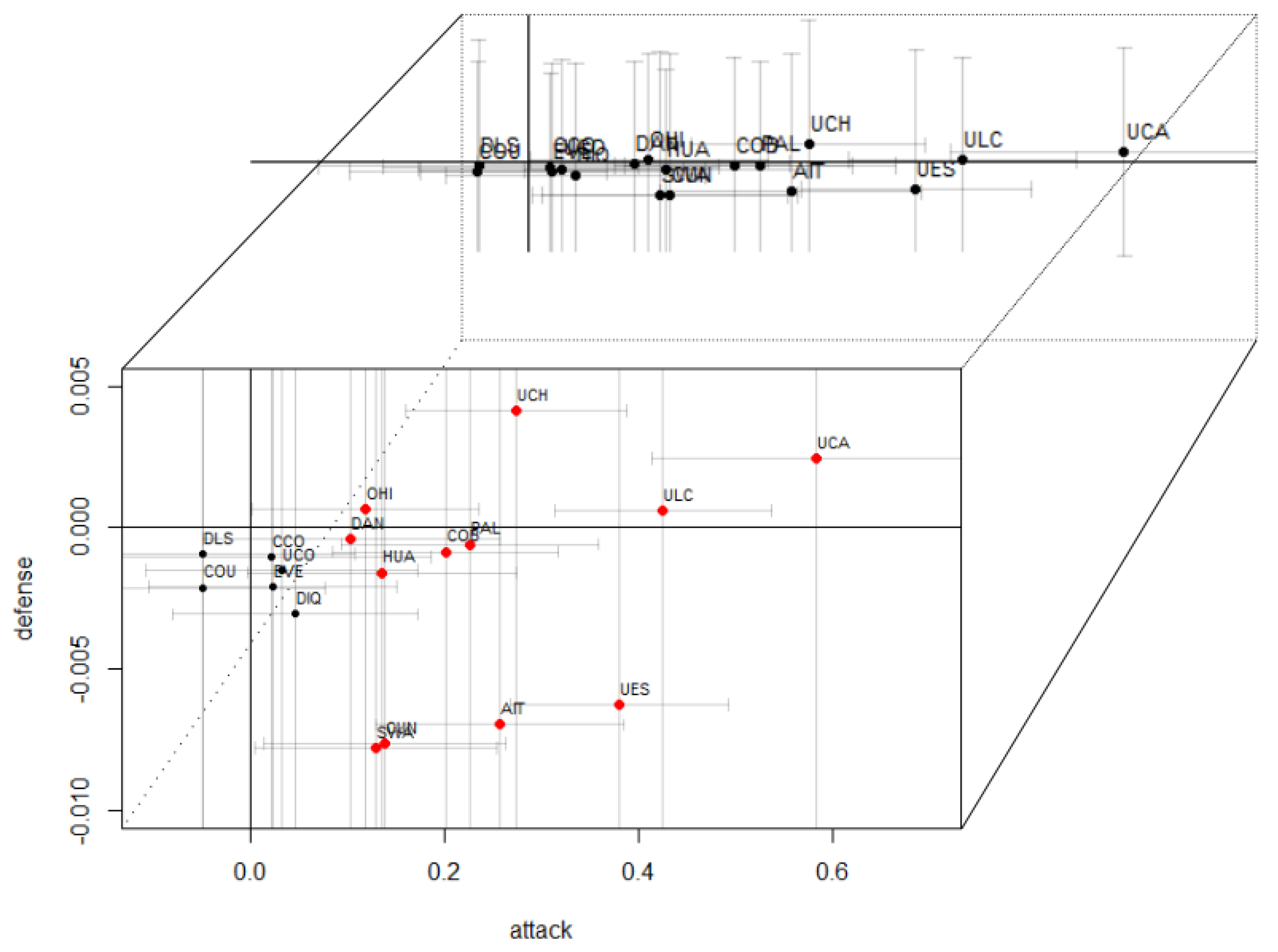
In
Figure 3, we are able to see the prediction of attack and defense of the 18 teams in the league, in which we can observe that the level of the defense for each team individually was statistically equal to zero, which means that there is no significant result in the defense among the teams. However, if it was obtained that the attack of the teams, such as the Universidad Católica (UCA), Unión La Calera (ULC) and Unión Española (UES), have greater attack power according to the model. In addition, the prediction error of the model is displayed, with regards to the attack prediction of the teams, that is, due to the size of the attack it is possible to present the championship positions, according to the adjusted Poisson regression model.
Additionally, from observation of
Figure 4, it is possible to notice the attack average of each team, and we can see that the first five teams with the highest attacking average are the same first five teams who have been better ranked at the end of the season, and positions 5 to 11 are also the same teams although not in the same position.
In
Table 2, in addition to the 11 teams that have a significant statistic, there is also the Audax Italiano, which has a significant value and is in position 6 of the prediction table, whereas it is in position 14 of the final table of the 2020 championship. However, its defense is one of the lowest, thus we can interpret this as an outlier.
Although most of the teams are between positions 11 and 18 of the final table of the championship, their attack and defense prediction errors are high compared to the other 11, which may lead to thinking that this is a factor that alters the program.
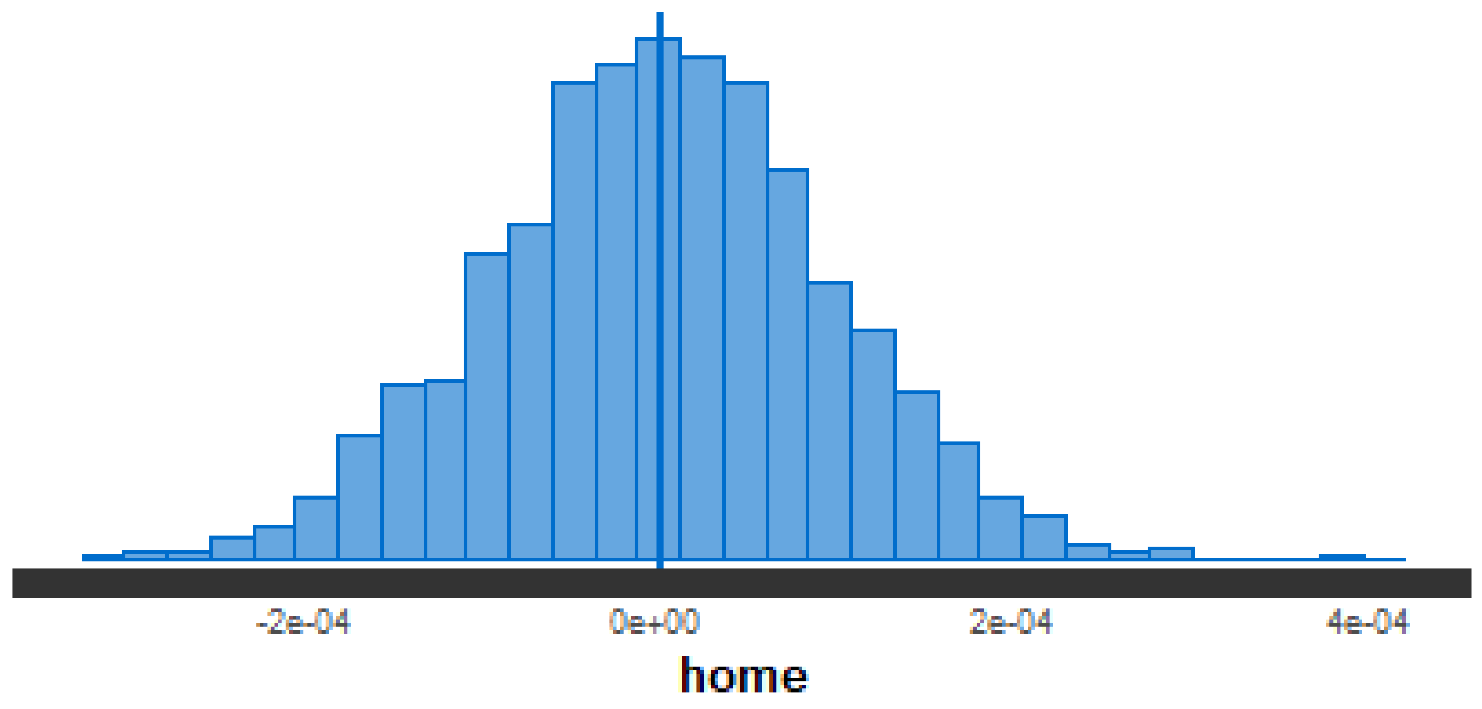
On the other hand, we can see in
Figure 5 how the
Home parameter is distributed, which represents the attack and defense of each team at home, and looks symmetrically distributed. In this way, we can say that the
Home parameter did not intervene in the definition of a match in the 2020 Chilean Premier League.
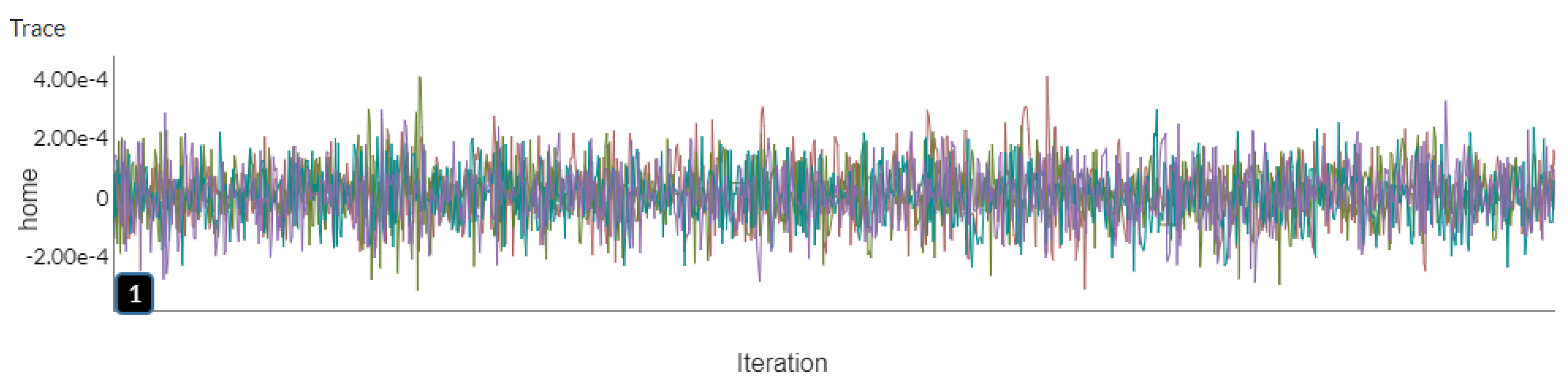
Figure 6 shows four HMC chains of the
Home parameter, in which in order to determine convergence it is convenient to observe that the four chains are consistent and to check that the chains are not stuck in unusual regions. Therefore, we can say that the chains converge.
We can also observe the deviation represented by and . For the case of defense, we have an asymmetry that is close to zero. On the other hand, for attack, we have an average of the dispersion between 0.2 and 0.3.
The use of the Shinystan package facilitates the analysis of the results due to the intuitive and easy interaction of this package, and by adopting the function, a parsing interface related to the strings from HMC, you will be able to view various graphs and parameter estimates in more detail.
One of the first visualizations would be the HMC chains adopted from the model, also allowing a separate or simultaneous display on the same graph. The HMC strings, approximated by the NUTS algorithm, are computationally more expensive than Metropolis or Gibbs. However, they are more efficient, and therefore the samples can be small [
24].
The convergence of the chains is intuitively represented when targeting the same region, that is, there is a behavior similar to a convergence point (value), and the variance between the chains is approximately equal to the mean variance within the chains (homoscedastic), also quantified by the estimated
(
) statistic, which is close to 1 [
24]. As an example of convergence of the
Home parameter,
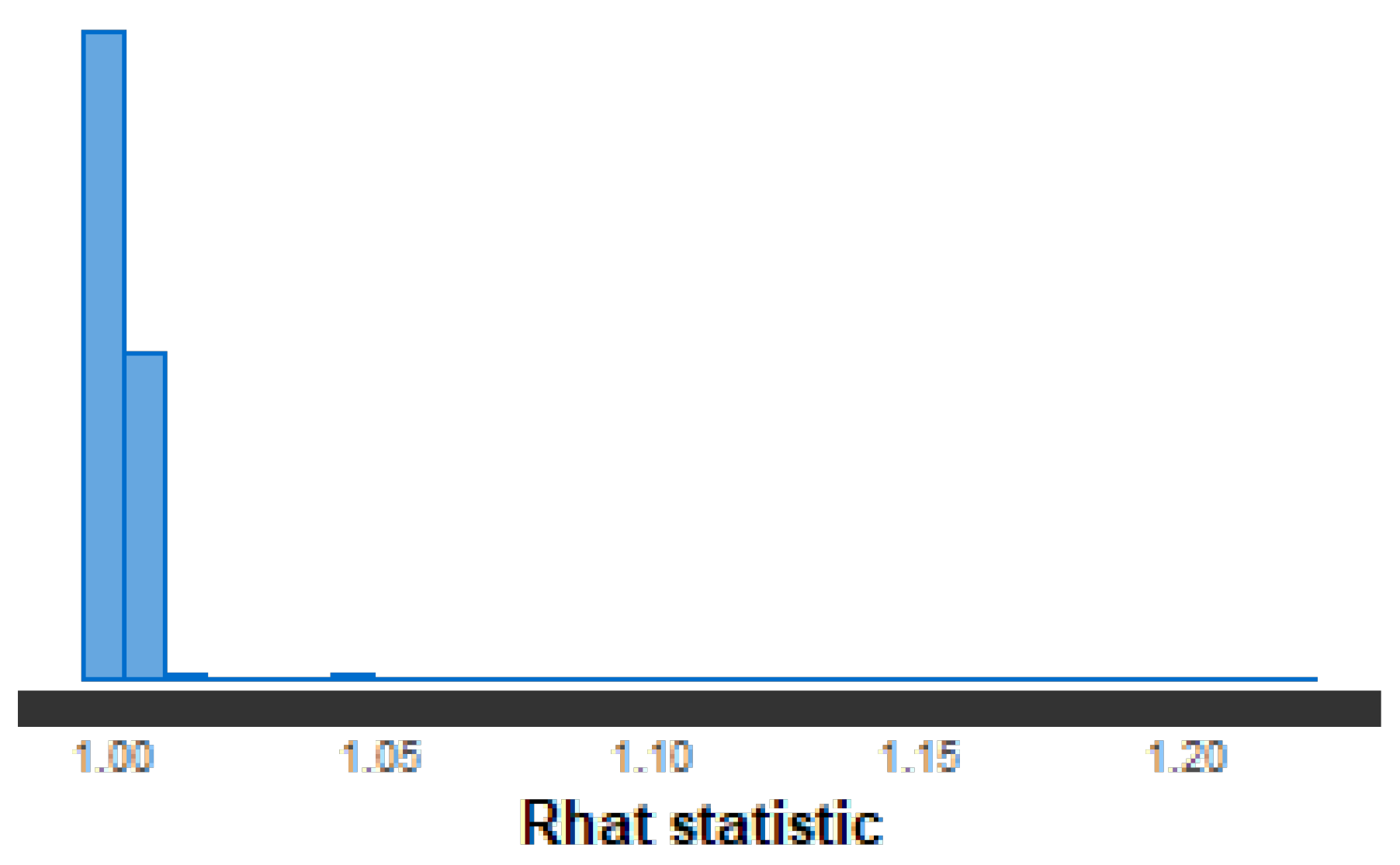
Figure 6 demonstrates the obtained strings in which each color refers to different strings, and the beginning of each chain was randomly selected from the Normal (0, 0.01) distribution. In addition, the chains look visually stationary achieving the convergence measure, showing just a random noise around the mode of the posterior for the
Home parameter, confirmed by the statistics of the
value concentrated at 1 (less than the threshold 1.01), as shown by
Figure 7.
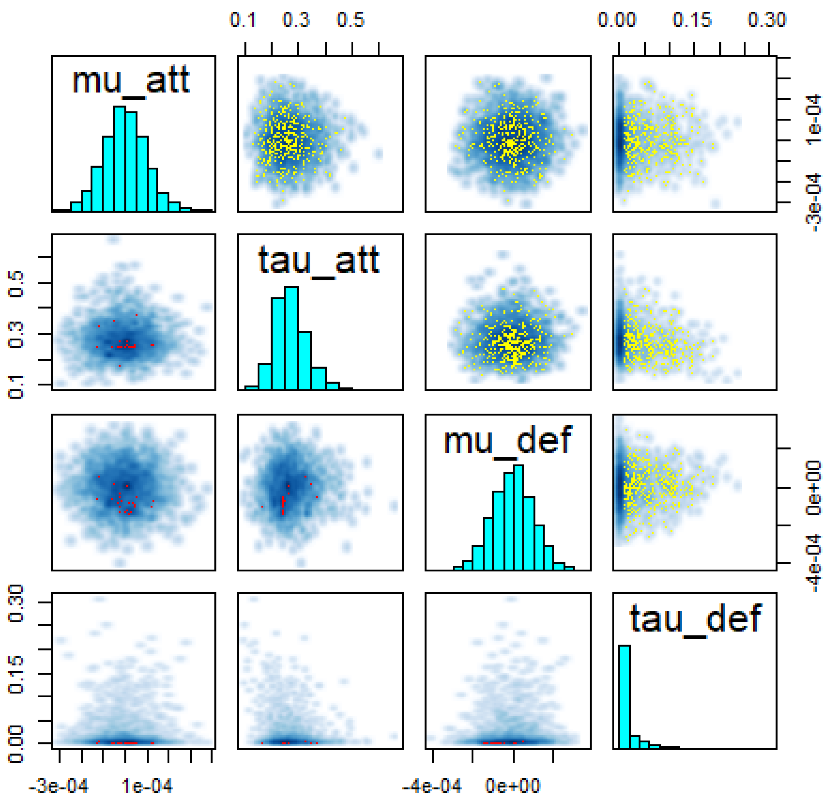
Shinystan also makes it possible to view all the posteriors of the parameters adopted by the statistical model, enabling a better understanding of what is being analyzed and, in the case of seeing any anomaly, to be able to correct it or to do some other test. For each parameter that intervenes in the model, a graph of the posterior distribution is generated, and, as shown in
Figure 8, the posterior distributions for the
,
,
and
parameters obtained by the HMC strings. From these graphs, we could see that the
Home parameter is distributed in a symmetric way (in
Figure 5), and that the
and
parameters have slight skewness (in
Figure 8). The precision parameters
and
are involved with attack parameter dispersion and suggest a significance, compared to defense, since the distribution of
is around zero.
In view of their empirical distributions,
Figure 8 shows that, in the upper triangle, there is no trend in the posterior parameters, which makes them look unrelated (
,
,
and
). It is also important to highlight that the parameter (
) can approximate a discussion related to the attacking average of the Chilean league (
) and the defense average in a way that represents the championship as the main one in Chile. Observing the figure, it is in accordance with the previous one since the defense average is zero, that is, it does not contribute to the prediction. However, the attack average is non-zero (specifically for some teams being statistically significant).
In the lower triangular part of
Figure 8, we see the predictive posterior of the parameters involved, from which we see that it adjusts to the expected values.
It can also be obtained individually, that is, per team, associated with the posterior distributions of defense and attack. This is an important aspect if you want to observe the performance of only one computer (obtained by adopting the hierarchical model).
Some of the metrics that were extracted from the
Shinystan interface are presented in
Table 3, in which the
metric validates the convergence of each of the strings in a general way, since there are values close to one.
The values are small. Therefore, the program performed long simulation times for the interval. In the case of treedepth, the values are different from zero and it does not hit the maximum value, which is shown to be an efficient No-U-Turn-Sampler.
The metrics of and were also extracted, indicating that the following parameters: , , , , , , , , log-posterior, have an effective sample size less than 10% of the total sample size; and that the following parameters: , , , , , have a Monte Carlo standard error greater than 10% of the posterior standard deviation. Finally, for the development of this research, the autocorrelation metric was necessary, which shows the relationship of the parameters in each of the strings, and after their analysis, all chains presented signals of convergence.
Our models predicted correctly most of the Chilean final ranking positions, using the last five matches for prediction.
Table 4 shows the median prediction, generated from the adjusted Poisson derived from the four independent chains which generated quantities blocks, based on both adopted models (hierarchical and non-hierarchical) which presented quite similar results.
For example, the first five positions predicted by the model are: Universidad Católica (UCA), Unión La Calera (ULC), Unión Española (UES), Universidad de Chile (UCH) and Palestino (PAL), in an order based on a calculated attack, whereas the general table remained: Universidad Católica (UCA), Unión La Calera (ULC), Universidad de Chile (UCH), Unión Española (UES) and Palestino (PAL), which, in the final table, is affected by the league rules that indicate that, at the time of equalizing the points, the position is defined by the goal difference, and since our model is based on the goals scored, it will show the one that scores more goals at the top of the table. The highest one in the table is the one that scores more goals. Therefore, by organising the attack value of the teams in decreasing order, and comparing with the final table of the league (
Table 5), our model manages to predict most of the positions exactly when it comes to the highlighted teams.
On the other hand, positions 7 to 12 of
Table 2, according to the estimates of the Poisson model, correspond to positions 6 to 11 of the final table of positions for the Chilean league (
Table 5). It happens that, since the difference between one position and the other is one point, then the positions predicted by model 2 were not equivalent to the final result.


 and
and 


