
Spark Configurations to Optimize Decision Tree Classification on UNSW-NB15


Department of Computer Science, University of West Florida, Pensacola, FL 32514, USA
*
Author to whom correspondence should be addressed.
Big Data Cogn. Comput. 2022, 6(2), 38; https://doi.org/10.3390/bdcc6020038
Submission received: 1 March 2022
/
Revised: 26 March 2022
/
Accepted: 4 April 2022
/
Published: 7 April 2022
Abstract
:This paper looks at the impact of changing Spark’s configuration parameters on machine learning algorithms using a large dataset—the UNSW-NB15 dataset. The environmental conditions that will optimize the classification process are studied. To build smart intrusion detection systems, a deep understanding of the environmental parameters is necessary. Specifically, the focus is on the following environmental parameters: the executor memory, number of executors, number of cores per executor, execution time, as well as the impact on statistical measures. Hence, the objective was to optimize resource usage and minimize processing time for Decision Tree classification, using Spark. This shows whether additional resources will increase performance, lower processing time, and optimize computing resources. The UNSW-NB15 dataset, being a large dataset, provides enough data and complexity to see the changes in computing resource configurations in Spark. Principal Component Analysis was used for preprocessing the dataset. Results indicated that a lack of executors and cores result in wasted resources and long processing time. Excessive resource allocation did not improve processing time. Environmental tuning has a noticeable impact.
1. Introduction
The goal of this paper was to observe the impact of adjusting Spark’s configuration parameters for decision tree classification using a large dataset. To build smart intrusion detection systems, a deep understanding of the environmental parameters is also necessary. The environmental conditions that will optimize the classification process are studied. Specifically, the focus is on the following environmental parameters: executor memory, number of executors, cores, and execution time. The objective was to find the optimal configuration settings needed to minimize memory usage and processing time for classification in Spark’s environment. Principal Component Analysis (PCA) was used for dimension reduction.
This internet day and age has brought a tremendous increase in computer network traffic. With this increase in computer network traffic has come an increase in malicious traffic, manifested as anomalies in regular network traffic [1], hence the need for efficient intrusion detection systems (IDSs) to detect malicious traffic early. A huge amount of computer network traffic has also brought an additional challenge of handling and analyzing large amounts of data quickly and efficiently. This paper looks at building intrusion detection systems (IDSs) using anomaly detection, availing of the decision tree classifier in the distributed Big Data Framework using Spark. Using a large dataset, UNSW-NB15 [2,3], the performance of running the decision tree classifier in the parallel Big Data environment, Spark, was tracked using the SparkUI. Spark, a parallel cluster computing framework that sits on top of the Hadoop Big Data Framework, gains its efficiency from having data and processes reside completely in-memory [4]. Additionally, Spark comes with a rich set of APIs that allow complex analytical operations to be performed out-of-the-box.
The decision tree classifier was used in this work so that the classifier results obtained in Spark’s parallel computing environment could be compared to previous studies done using the traditional decision tree classifier on the UNSW-NB15 dataset. The decision tree classifier has previously been used for classification in IDSs by many [5,6,7,8], giving high detection accuracy without compromising learning speed. Refs. [5,6] also used the decision tree classifier on the UNSW-NB15.
2. Related Works
Several works have studied the application of various machine learning techniques on several different intrusion detection datasets. Since there are minimal resources that study the Spark environment in the context of environmental parameters [7,8], the majority of related works focus on similar statistical measures and decision tree classification on intrusion detection datasets—specifically, the UNSW-NB15 dataset.
Mostafaeipour et al. [7] compared and evaluated the KNN algorithm within Hadoop and Spark. The runtime of spark was 4 to 4.5 times faster than Hadoop. The memory usage in Hadoop was less than Spark.
Chang et al. [8] proposed the Hyperband algorithm to optimize the Spark parameters and improve the efficiency of the Spark platform. Using the Hyperband algorithm, the parameter model is trained through historical data information. The Spark parameter model was chosen for different job requirements. With 5 GB dataset, this method reduced the job execution time by approximately 12.94%.
Gao et al. [9] proposed a neural network algorithm, I-ELM, which improved detection accuracy and training speed. These authors combined adaptive PCA to extract effective features automatically. Being adjustable, in I-ELM, nodes could be added to solve underfitting and overfitting. To prove the method’s efficiency, the paper compared SVM, BP, CNN, ELM, and I-ELM on the NSL-KDD and UNSW-NB15 datasets. Despite the imbalanced distribution of data among the attack types in the NSL-KDD dataset, and the large numbers of new network attack types in UNSW-NB15, I-ELM, combined with adaptive PCA, showed the highest detection accuracy and the lowest false alarm rates.
Qiao et al. [10] proposed a Direct Linear Discriminant Analysis (DLDA) and PCA to obtain detection rates (DR) and false alarm rates (FAR) at an acceptable level on UNSW-NB15. To solve the small sample size (SSS) problem and lack of discriminant information, the authors used Discriminative PCA (DPCA). Detection was implemented using the simple nearest-neighbor (NN) classifier. For multi-classes, PCA and DPCA gave similar results. For binary-class detection, DPCA outperformed DLDA and PCA in accuracy, DR, and FAR.
Moustafa et al. [11] proposed a threat intelligence architecture evaluating a CPS data set of sensors and actuators and the UNSW-NB15 data set of network traffic based on Beta Mixture and Hidden Markov Models (MHMM). In order to improve MHMM performance, Independent Component Analysis (ICA) was used to reduce data dimensionality. Beta Mixture Model (BMM) was used for fitting multivariate time series. Accuracy, Detection Rate, and False Alarm Rate were used to measure the performance between the techniques, MHMM, Cart, KNN, SVM, RF, and OGM, on the CPS and UNSW-NB15 datasets. MHMM performed better than the other techniques on both the datasets and was more efficient in recognizing different normal and abnormal records.
Sheshasaayee et al. [12] compared Decision Tree, Random Forest, and Gradient Boosting Tree in the native MapReduce and Spark frameworks over the parameters read, write, time, and space. The authors found that all the tree-based algorithms performed much better on the Spark framework than the native MapReduce.
Belouch et al. [13] compared SVM, Naïve Bayes, Decision Tree, and Random Forest, for classification accuracy, sensitivity, specificity and execution time on the UNSW-NB15 dataset. Decision tree had an accuracy of 85.56% and FAR of 15.78%. Random Forest had a specificity at 97.49%, and the specificity of Decision Tree was 97.10%. Random Forest had a slightly higher accuracy at 97.49% compared to 95.82% but took longer to train at 5.69 s compared to 4.30 s. Both performed far better than SVM and Naïve Bayes. In conclusion, Random Forest was slightly better at detection on all types of network traffic.
Koroniotis et al. [14] tested four classification techniques used to recognize attack vectors in IoT devices—Decision Tree (DT), Association Rule Mining (ARM), Artificial Neural Network (ANN), and Naïve Bayes (NB). An Information Gain Ranking Filter (IG) selected the 10 highest-ranked features. The metrics used for the determination of success of each algorithm where accuracy and False Alarm Rate (FAR). This study showed that the DT Classifier was the best for recognizing differences in Botnet and normal traffic. ANN were the least successful.
Moustafa et al. [15] applied Naïve Bayes, Decision Tree, Artificial Neural Network, Logistic Regression, and Expectation-Maximization (EM) clustering techniques to UNSW-NB15 and KDD99 to analyze the accuracy and false alarm rate. On the UNSW-NB15 data set, decision tree gave the highest accuracy and lowest FAR; EM clustering resulted in the lowest accuracy and highest FAR.
Kasongo and Sun [16] compared Support Vector Machine, k-Nearest-Neighbor, Logistic Regression, Artificial Neural Network, and Decision Tree performance after applying XGBoost algorithm, a filter-based feature reduction technique on UNSW-NB15 dataset. The results showed that Decision Tree had a better test accuracy compared to other Machine Learning algorithms. XGBoost helped improve Decision Tree prediction.
Kumar et al. [6] proposed an integrated classification-based model using the UNSW-NB15 dataset as an offline dataset. A real-time dataset (RTNITP18) was generated as a testing dataset on a proposed model. Different existing decision tree models (C5, CHAID, CART, and QUEST) were compared to the proposed integrated model, showing higher performance in detection rate and FAR. The proposed integrated rule-based model kept the highest confidence factors to be used for the rule-based model.
Though there are several works using the decision tree classifier on UNSW-NB15, and some of them also use Spark, except for [7,8], none of the works have looked at optimizing the Spark configuration parameters to get better results using the decision tree classifier on the UNSW-NB15 dataset, which is the focus of this work. And [7,8] did not specifically use the decision tree classifier.
3. The UNSW-NB15 Dataset
UNSW-NB15 [2,3] was created by the IXIA Perfect Storm tool1 in the Cyber Range Lab of the Australian Centre for Cyber Security (ACCS) in conjunction with UNSW Canberra, Australia [13]. This dataset is a fusion of actual modern normal network traffic and contemporary synthesized attacks [14]. 100 GB of raw data was used to generate a hybrid of real and synthetic data to simulate contemporary attack behaviors. The dataset is made up of four separate files that contain 2,540,047 separate lines of data at 559.3 MB of CSV data. This includes 49 different variables, including Label, which defines each instance as benign traffic or as an attack. Attack_cat categorizes the type of attack.
When combining the four separate data files into one, there were a few cleaning issues: extra spaces had to be trimmed in a few columns and two versions of an attack category, with/without an -s were present. Columns that contained null values were converted using StringIndexer() prior to transforming into PCA.
This dataset tracks nine types of attacks, as shown in Figure 1. The attacks are Analysis, Backdoors, DoS, Exploits, Reconnaissance, Shellcode, Worms, Fuzzers, and Generic. Figure 2 shows the distribution of benign versus attack traffic.
Analysis, as in traffic analysis, are eavesdropping attacks designed to listen to network communications to infer the location of key nodes, routing structure, network, infrastructure topology, and even application behavior patterns. Backdoor attacks are typically malware installations that negate normal authentication procedures to a system and allow remote access to an unauthorized person or agent. DoS, “denial of service”, are attacks that aim to make a server, service, or another part of the infrastructure unavailable, usually by overloading bandwidth to slow down or stop normal operations. Exploits are types of attacks that target a known or emerging vulnerability and weakness in an application, network, operating system, or hardware. Reconnaissance is a general knowledge gathering attack that can be both logical and physical. This can include sniffing, scanning, and phishing. Shellcode is a type of code attack where code is injected remotely. This allows software vulnerabilities to be exploited. It also allows the opening of remote instances of command line interpreters to further interact with infected systems. Worms are a type of self-replicating malware that can spread across systems and networks without human engagement; they can be first introduced by a human actor but then self-sustain and propagate automatically. Fuzzer attacks are designed to stress an application to cause unexpected behavior, resource leaks, or crashes. Generic is a catch-all class of attacks that do not fit strongly into one of the other types of attack [17].
4. Analysis Environment
4.1. Spark
Spark, a general-purpose advanced execution engine that can handle batch processing, interactive analysis, streaming data, machine learning, and graph computing, is an in-memory cluster computing framework for processing and analyzing large amounts of data [4]. This type of programming interface has become crucial as the need to process large datasets has continued to grow. Rather than writing to the disk every time, Spark caches data in memory and only writes to the disk one time. Additional characteristics of Spark that make it powerful are simple to use, fast, general purpose, scalable, and fault tolerant. With the wide array of data processing jobs that Spark can handle, it was built to be scalable. To increase the capacity of a Spark cluster, all that has to be done is to add more nodes to the cluster [4]. Lastly, Spark, as previously mentioned, is fault tolerant, meaning that it automatically handles node failure without breaking the application. As a result, Spark can process tremendous amounts of data quickly and efficiently.
4.2. Principle Component Analysis
Though Spark can process large amounts of data, there is often still a need to reduce the dimensionality of data. This can be done through Principal Component Analysis or PCA. PCA is a statistical method for reducing a large set of possibly correlated variables to a smaller set of uncorrelated variables, known as principal components. In terms of Big Data analytics, PCA’s goal “is to find the fewest number of variables responsible for the maximum amount of variability in the dataset” [4]. Each principal component has the largest variance under the constraint that it is uncorrelated to the previous components.
4.3. Decision Tree
The decision tree algorithm infers a set of decision rules from a training dataset and creates a decision tree that can be used to predict the numeric label for an observation. The tree uses a hierarchy of nodes and edges. A decision tree is unlike a graph since there are no loops; a non-leaf node is called an internal or split node whereas a leaf node is called a terminal node. The decision tree algorithm starts at the root node and works its way down the tree until it reaches a terminal node. The decision tree algorithm “performs a series of tests on the features to predict a label” [4]. Though a decision tree can be used for both regression and classification, in this work the decision tree is used for classification.
5. Methodology
Figure 3 presents a flow diagram for the overall methodology used in this work. Although doing the PCA every time appears redundant at first glance, since SparkUI is used, we had to completely leave the Spark environment each time. Hence, PCA has to be re-done every single time.
Environmental Variables Used in Spark
Table 1 shows the environmental variables that were adjusted in the Spark runs.
In the Spark-shell, the number of executors, cores and memory allocated to the executors were varied using the statement:
- spark-shell—num-executors X—executor-cores X—executor-memory X
- Where X is a numeric value entered.
Core Spark classes in Scala [19] were used to perform all tasks. The Machine Learning library (mllib) and the sql class were used. Within the classes, the following were imported:
- org.apache.spark.sql.SparkSession
- org.apache.spark.ml.linalg.Vectors
- org.apache.spark.ml.feature.{VectorAssembler, VectorIndexer, StringIndexer, OneHotEncoder}
- org.apache.spark.ml.feature.{IndexToString, StringIndexer, VectorIndexer}
- org.apache.spark.ml.feature.PCA
- org.apache.spark.ml.Pipeline
- org.apache.spark.ml.classification.LogisticRegression
- org.apache.spark.ml.classification.DecisionTreeClassificationModel
- org.apache.spark.ml.classification.DecisionTreeClassifier
- org.apache.spark.ml.evaluation.MulticlassClassificationEvaluator
- org.apache.spark.mllib.evaluation.BinaryClassificationMetrics
- org.apache.spark.mllib.evaluation.MulticlassMetrics
A Spark session was built using SparkSession.builder(). This allowed the performance to be tracked and monitored in SparkUI to see the impact of the changing environmental variables. Spark UI was used to track the performance of the different Spark configuration parameters on the decision tree classifier. In Spark Application UI, stages in each Spark Job, tasks in each stage including summary metrics for completed tasks, aggregated metrics by executor, Resilient Distributed Dataset (RDD) storage, and environment can be monitored. Directed Acylic Graph (DAG) visualization and event timeline of each stage can be observed. From the application web UI Storage tab, each RDD storage displays partitions, memory usage, storage level, and executor IDs of each RDD partition. Spark runtime information, system properties, and class path entries can be monitored from the environment tab in the application web UI. Executors page provides all the information about active and dead executors, monitor logs, and executor threads [4]. The UNSW-NB15 dataset [13] was imported as comma separated values into the Hadoop File System. Since the dataset [13] was multiple files, they were merged into a vector column using the VectorAssembler class [19] to create a list of column names from the dataset to be used by the code. The transformed dataset from the VectorAssembler class transform method was used by the PCA class to produce a reduced dimension dataset from principal components. The data was randomly split into 70% training data observations and 30% testing observations using the random split method from the PCA Model class [19]. Finally, the decision tree classifier was run using the default settings from the DecisionTreeClassifier class [19].
This work was performed on a GHz 6-Core i7 16 GB 512 SSD machine. The work was performed using the Spark API, Spark ML, using the out-of-box PCA and decision tree algorithms, permitting fast data processing that is durable and robust. Lastly, it is important to note that the same block of code was used for each trial with the only change being the varying number of executors, cores, and memory allocated before each trial run.
6. Results and Discussion
Table 2 show the tabulated results of 11 runs with various combinations of Spark’s environment variables. Performance was evaluated in two ways: (i) cores and execution time based on memory used; and (ii) statistical metrics.
6.1. Performance Based on Cores and Memory versus Execution Time
10 executors and 2 cores and 10 executors and 6 cores offered the best results. As can be observed from Table 2, after running additional trials (runs 5–8—note that run 7 was a rerun of run 3, but without specifying executor memory, and run 8 was a rerun of run 4, without specifying executor memory), it can be noted that a significant number of dead cores were obtained for each run. This was because: for the original runs, spark-shell --num-executors # --executor-cores # --executor-memory 19 G was used, whereas in runs 5–8, spark-shell --num-executors 10 --executor-cores 6 was used. Hence, additional runs were performed using the business concept of ceteris paribus or “other things equal”—keeping the number of executors at 10 and cores at 6, but changing the executor memory each time. This allowed us to see the impact of adjusting the executor memory. These results are presented in Table 2. From runs 9–11, it can be noted that using 5 GB executor memory provided similar time.
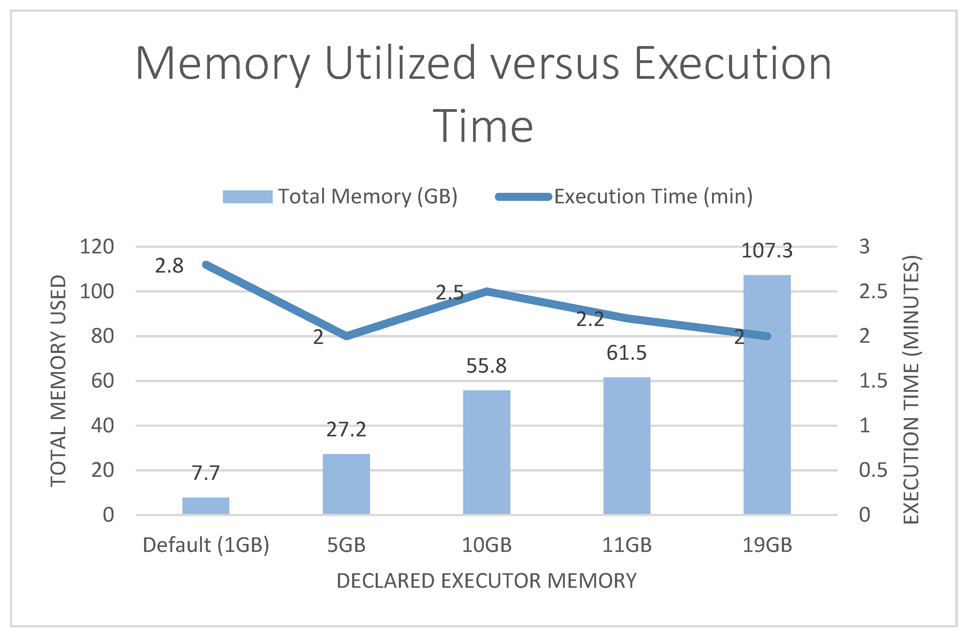
Figure 4 and Figure 5 present a comparison of results. These figures show a comparison for all runs with executors set to 10 and cores set to 6. The difference between each run is the executor memory that was declared upon launch of spark-shell. The executor memory specifications were as follows: default, 5 GB, 10 GB, 11 GB, and 19 GB. From Figure 4, it can be noted that the higher the declared executor memory, the higher the total memory, but execution time was high at the default executor memory of 1 GB and 10 GB. From Figure 5 it can be noted that higher declared executor memory used less cores (the number of cores remained consistent after 5 GB) and execution time was high only at the default of 1 GB and 10 GB.
6.2. Performance Based on Statistical Metrics
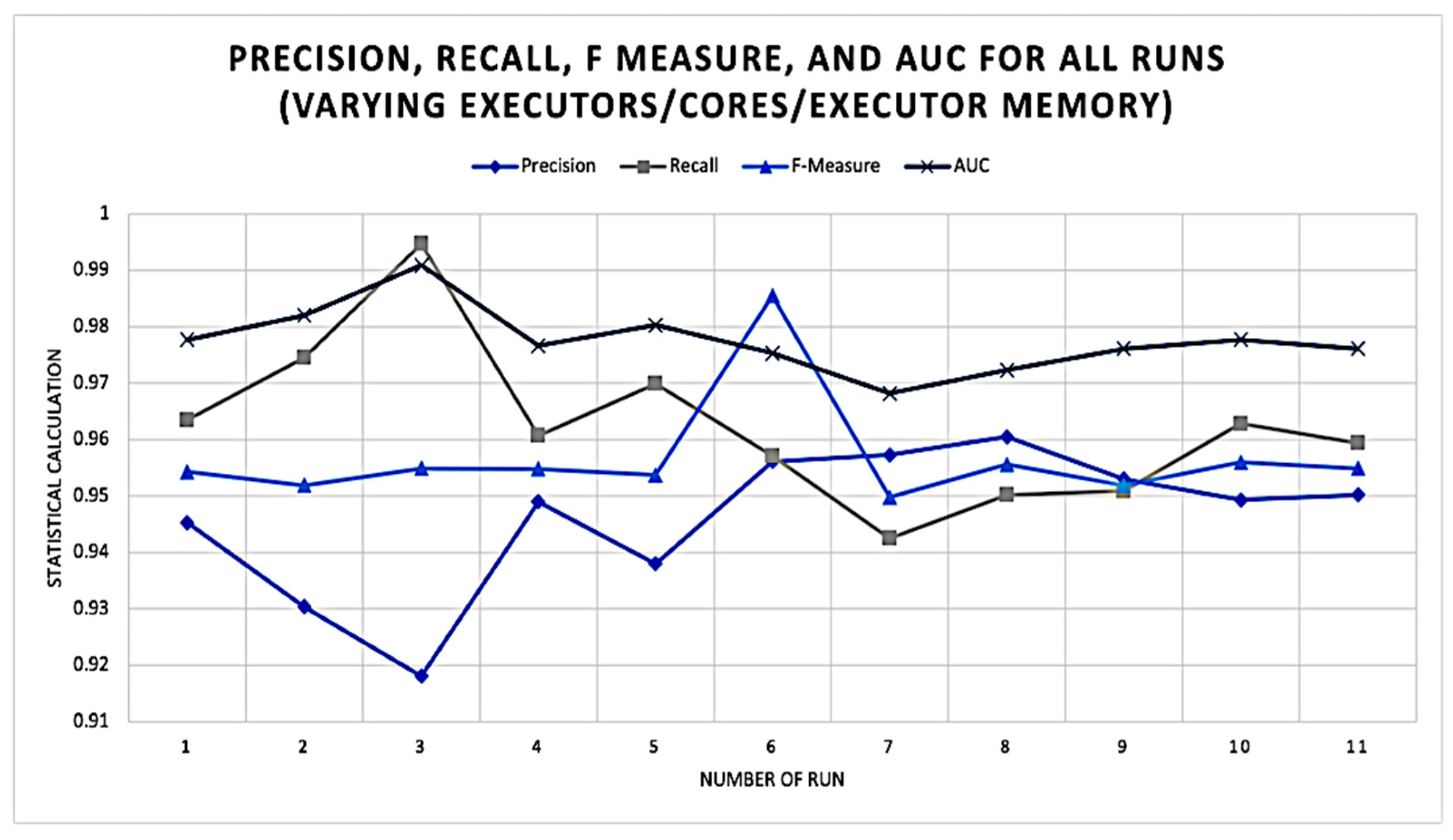
In addition to monitoring performance for each of the runs, the Accuracy, Precision, Recall, False Alarm Rate (FAR), F-measure, and AUC Area Under the Curve (AUC) was recorded for all 11 runs.
Accuracy is the ratio of a model’s correct data (TP + TN) to the total data, calculated by:
Accuracy = (TP + TN)/(TP + TN + FP + FN)
Precision is the ratio of true positives to all positives, determined by:
Precision = TP/(TP + FP)
Recall is the fraction of the positive examples classified correctly by a model:
Recall = TP/(TP + FN)
False Alarm Rate (FAR) or False Positive Rate is the ratio of the number of negative events wrongly categorized as positive to the total number of actual negative events. FAR is given by:
FAR = FP/(FP + TN)
F-measure is the harmonic mean of the recall and precision of a model:
F-measure = (2 ∗ precision ∗ recall)/(precision + recall)
Note: TP stands for “True Positives”, FN stands for “False Negatives”, and FP stands for “False Positives”.
From Table 3, it can be noted that the number of cores and executors specified did not impact the statistical calculations. Figure 6 demonstrates that for each of the runs while varying the number of executors, cores, and executor memory, the ranges for each of the statistical measures were fairly consistent, on average. Precision ranged from 0.9181 to 0.9605. Recall ranged from 0.9425 to 0.9947. F-measure ranged from 0.9498 to 0.9855. AUC ranged from 0.9682 to 0.9909.
Table 4 presents classification results of using the decision tree algorithm on UNSW-NB15. The last row shows the results obtained by our parallel implementation of Spark. The last line—our results—are an average of the 11 runs that were performed. As per Table 3, in terms of FAR, as well as accuracy, decision tree used in Spark’s parallel framework did a lot better than previous uses of the decision tree algorithm. Most importantly, the total execution time was a lot lower after tuning Spark’s parameters.
This work clearly demonstrates that adding additional resources does not guarantee better performance. On one hand, if too few resources are used along with a large dataset, it will result in numerous dead cores. On the other hand, a significant increase in resources did not prove to provide any significant performance time benefits. In the real world this would be an expensive waste of resources because of the additional cost associated with using a larger amount of resources.
7. Conclusions
In this work, different executor memory sizes were compared on different memory ranges from 1 GB to 19 GB using different numbers of executors and cores. The results point out some key performance indicators, including explicitly assigning executor memory to avoid dead cores, in some cases extended processing time. That is, a lack of executors and cores result in a significant time increase, dead cores, and unacceptably long processing time. Hence the results showed the optimal combination which minimizes both memory used and processing time. The overall conclusion is that as the declared executor memory increased the executive time went down, but the number of cores remained the same. Finally, the decision tree algorithm on Spark’s parallel environment performed better in terms of classification time, accuracy, and False Alarm Rate.
8. Future Works
Spark 2.x was used for the content of this paper; all the referenced works also used this CPU focused version of Spark. With the release of Spark 3.x [20] columnar processing support is provided in Spark’s Catalyst query optimizer—the logical query plan optimizer, which can accelerate DataFrame operations [21] using Graphics Processing Unit (GPU) resources on the Spark clusters. NVIDIA [21] states that Spark on NVIDIA GPUs will reduce infrastructure costs by completing jobs faster with less hardware compared to the CPU based alternative. It would be interesting to see if these claims can be proven with this research conducted in a Spark 3.x environment. All these trials could be conducted in the upgraded environment and tested to see the impact of allocating more GPU cores instead of CPU along with the executors and memory maintained at constant levels for both does decrease the runtimes reported in this work.
Author Contributions
Conceptualization, S.B. (Sikha Bagui); methodology, S.B. (Sikha Bagui); software, M.W., R.D., H.P. and S.B. (Shaunda Boucugnani); validation, S.B. (Sikha Bagui), M.W., R.D., H.P. and S.B. (Shaunda Boucugnani); formal analysis, S.B. (Sikha Bagui), M.W., R.D., H.P. and S.B. (Shaunda Boucugnani); investigation, S.B. (Sikha Bagui), M.W., R.D., H.P. and S.B. (Shaunda Boucugnani); resources, S.B. (Sikha Bagui), M.W., R.D., H.P. and S.B. (Shaunda Boucugnani); data curation, M.W., R.D., H.P. and S.B. (Shaunda Boucugnani); writing—original draft preparation, S.B. (Sikha Bagui), M.W., R.D., H.P. and S.B. (Shaunda Boucugnani); writing—review and editing, S.B. (Sikha Bagui), M.W., R.D., H.P. and S.B. (Shaunda Boucugnani); visualization, S.B. (Sikha Bagui), M.W., R.D., H.P. and S.B. (Shaunda Boucugnani); supervision, S.B. (Sikha Bagui); project administration, S.B. (Sikha Bagui). All authors have read and agreed to the published version of the manuscript.
Funding
This research received no external funding.
Institutional Review Board Statement
Not Applicable.
Informed Consent Statement
Not Applicable.
Data Availability Statement
The Data is available at: https://research.unsw.edu.au/projects/unsw-nb15-dataset (accessed on 3 April 2022).
Conflicts of Interest
The authors declare no conflict of interest.
References
- Bagui, S.; Simonds, J.; Plenkers, R.; Bennett, T.; Bagui, S. Classifying UNSW-NB15 Network Traffic in the Big Data Framework using Random Forest in Spark. Int. J. Big Data Intell. Appl. 2021, 2, 17. [Google Scholar] [CrossRef]
- The UNSW-NB15 Dataset Description. Cyber Range Lab of the Australian Centre for Cyber Security (ACCS). Available online: https://www.unsw.adfa.edu.au/unsw-canberra-cyber/cybersecurity/ADFA-NB15-Datasets/. (accessed on 19 September 2019).
- Moustafa, N.; Slay, J. UNSW-NB15: A comprehensive data set for network intrusion detection systems (UNSW-NB15 network data set). In Proceedings of the Military Communications and Information Systems Conference (MilCIS), Canberra, Australia, 10–12 November 2015. [Google Scholar] [CrossRef]
- Guller, M. Big Data Analytics with Spark: A Practitioner’s Guide to Using Spark for Large Scale Data Analysis, 1st ed.; Apress: New York, NY, USA, 2015. [Google Scholar]
- Kasongo, M.S.; Sun, Y. Performance Analysis of Intrusion Detection Systems Using a Feature Selection Method on the UNSW-NB15 Dataset. J. Big Data 2020, 7, 105. [Google Scholar] [CrossRef]
- Kumar, V.; Sinha, D.; Das, A.K.; Pandey, S.C.; Goswami, R.T. An integrated rule based intrusion detection system: Analysis on UNSW-NB15 data set and the real time online dataset. Clust. Comput. 2019, 23, 1397–1418. [Google Scholar] [CrossRef]
- Mostafaeipour, A.; Jahangard Rafsanjani, A.; Ahmadi, M.; Arockia Dhanraj, J. Investigating the performance of Hadoop and Spark platforms on machine learning algorithms. J. Supercomput. 2020, 77, 1273–1300. [Google Scholar] [CrossRef]
- Chang, D.; Qiao, Z.; Li, L.; Zheng, Q. Parameter Optimization of Spark in Heterogeneous Environment Based on Hyperband. In Proceedings of the 2021 2nd International Conference on Big Data Economy and Information Management (BDEIM), Sanya, China, 3–5 December 2021; pp. 204–208. [Google Scholar] [CrossRef]
- Gao, J.; Chai, S.; Zhang, B.; Xia, Y. Research on Network Intrusion Detection Based on Incremental Extreme Learning Machine and Adaptive Principal Component Analysis. Energies 2019, 12, 1223. [Google Scholar] [CrossRef] [Green Version]
- Qiao, H.; Blech, J.; Chen, H. A Machine learning based intrusion detection approach for industrial networks. In Proceedings of the IEEE International Conference on Industrial Technology (ICIT), Buenos Aires, Argentina, 26–28 February 2020; pp. 265–270. [Google Scholar] [CrossRef]
- Moustafa, N.; Adi, E.; Turnbull, B.; Hu, J. A New Threat Intelligence Scheme for Safeguarding Industry 4.0 Systems. IEEE Access 2018, 6, 32910–32924. [Google Scholar] [CrossRef]
- Sheshasaayee, A.; Lakshmi, J.V.N. An insight into tree-based machine learning techniques for big data analytics using Apache Spark. In Proceedings of the International Conference on Intelligent Computing, Instrumentation and Control Technologies (ICICICT), Kerala, India, 6–7 July 2017; pp. 1740–1743. [Google Scholar] [CrossRef]
- Belouch, M.; El Hadaj, S.; Idhammad, M. Performance evaluation of intrusion detection based on machine learning using Apache Spark. Procedia Comput. Sci. 2018, 127, 1–6. [Google Scholar] [CrossRef]
- Koroniotis, N.; Moustafa, N.; Sitnikova, E.; Slay, J. Towards Developing Network Forensic Mechanism for Botnet Activities in the IoT Based on Machine Learning Techniques. In International Conference on Mobile Networks and Management; Springer: Cham, Switzerland, 2018. [Google Scholar] [CrossRef] [Green Version]
- Moustafa, N.; Slay, J. The evaluation of Network Anomaly Detection Systems: Statistical analysis of the UNSW-NB15 data set and the comparison with the KDD99 data set. Inf. Secur. J. 2016, 25, 18–31. [Google Scholar] [CrossRef]
- Bagui, S.; Benson, D. Android Adware Detection Using Machine Learning. Int. J. Cyber Res. Educ. 2021, 3, 1–19. [Google Scholar] [CrossRef]
- Simmons, C.; Shiva, S.; Bedi, H.; Dasgupta, D. AVOIDIT: A cyber attack taxonomy. In Proceedings of the 9th Annual Symposium on Information Assurance (ASIA’14), Albany, NY, USA, 3–4 June 2014; pp. 2–12. [Google Scholar]
- Alibaba Cloud. Configure Spark-Submit Parameters—EMR Development Guide | Alibaba Cloud Documentation Center. Available online: https://www.alibabacloud.com/help/en/doc-detail/28124.html (accessed on 10 January 2020).
- Spark.apache.org. Overview—Spark 2.4.0 Documentation. 2022. Available online: https://spark.apache.org/docs/2.4.0/ (accessed on 15 March 2022).
- Spark.apache.org. Spark Release 3.0.0 | Apache Spark. 2022. Available online: https://spark.apache.org/releases/spark-release-3-0-0.html (accessed on 15 March 2022).
- NVIDIA. NVIDIA Apache Spark 3.0 For Analytics & ML Data Pipelines. 2022. Available online: https://www.nvidia.com/en-us/deep-learning-ai/solutions/data-science/apache-spark-3/ (accessed on 15 March 2022).
Figure 1.
Distribution of Network Attack Types.

Figure 2.
Distribution of Benign versus Attacks.

Figure 3.
Flow Diagram for Methodology.

Figure 4.
Executor Memory versus Execution Time and Total Memory.

Figure 5.
Cores versus Execution Time and Total Cores Used.

Figure 6.
Precision, Recall, F-Measure, and AUC Calculations for all runs (varying executors/cores/executor memory).
Figure 6.
Precision, Recall, F-Measure, and AUC Calculations for all runs (varying executors/cores/executor memory).


Table 1.
Environment Variables [18].
Table 1.
Environment Variables [18].
| Environment Variables | Function |
|---|---|
| --num-executors | The number of executors to be created |
| --executor-cores | The number of threads used by each executor, which equals the maximum number of tasks that can be executed concurrently by each executor |
| --executor-memory | The maximum amount of memory to be allocated to each executor. The allocated memory cannot be greater than the maximum available memory per node |
Table 2.
All Trial Runs.
| Run | # of Executors # of Executor Cores | Executor Memory | Cores Used | Dead Cores | Execution Time (min) | Memory Used (GB) | Spark Jobs Run | # of Executors | Completed Tasks | Dead Tasks | Read/Write (MB) |
|---|---|---|---|---|---|---|---|---|---|---|---|
| 1 | Executors: 4 Cores: 4 | 19 GB | 8 | 16 | 6.9 | 64.6 | 37 | 6 | 1151 | 17.5 | |
| 2 | Executors: 5 Cores: 2 | 19 GB | 12 | 0 | 3.5 | 64.5 | 37 | 6 | 621 | 13.5 | |
| 3 | Executors: 10 Cores: 2 | 19 GB | 24 | 0 | 3.0 | 128.7 | 37 | 12 | 1183 | 17.4 | |
| 4 | Executors: 10 Cores: 6 | 19 GB | 60 | 0 | 2.0 | 107.3 | 37 | 10 | 3017 | 27.5 | |
| 5 | Executors: 12 Cores: 5 | Default—1 GB | 80 | 45 | 2.5 | 6.8 | 37 | 16 | 3012 | 2188 | 28.2 |
| 6 | Executors: 8 Cores: 5 | Default—1 GB | 65 | 40 | 2.7 | 5.4 | 37 | 12 | 1996 | 1964 | 22.7 |
| 7 | Executors: 10 Cores: 2 | Default—1 GB | 30 | 10 | 3.1 | 6.3 | 37 | 15 | 1205 | 518 | 17.9 |
| 8 | Executors: 10 Cores: 6 | Default—1 GB | 108 | 54 | 2.8 | 7.7 | 37 | 18 | 3017 | 2405 | 27 |
| 9 | Executors: 10 Cores: 6 | 10 GB | 60 | 0 | 2.5 | 55.8 | 37 | 10 | 3017 | 28.4 | |
| 10 | Executors: 10 Cores: 6 | 11 GB | 60 | 0 | 2.2 | 61.5 | 37 | 10 | 3017 | 27 | |
| 11 | Executors: 10 Cores: 6 | 5 GB | 60 | 0 | 2.0 | 27.2 | 37 | 10 | 3017 | 27.4 |
Table 3.
Statistical Measures.
| Run # | # of Executors # of Executor Cores | Executor Memory | Precision | Recall | F Measure | AUC |
|---|---|---|---|---|---|---|
| Run 1 | Executors: 4 Cores: 4 | 19 GB | 0.9453 | 0.9635 | 0.9543 | 0.9777 |
| Run 2 | Executors: 5 Cores: 2 | 19 GB | 0.9304 | 0.9745 | 0.9947 | 0.9607 |
| Run 3 | Executors: 10 Cores: 2 | 19 GB | 0.9543 | 0.9519 | 0.9549 | 0.9548 |
| Run 4 | Executors: 10 Cores: 6 | 19 GB | 0.9777 | 0.982 | 0.9909 | 0.9766 |
| Run 5 | Executors: 12 Cores: 5 | Default—1 GB | 0.938 | 0.9699 | 0.9537 | 0.9803 |
| Run 6 | Executors: 8 Cores: 5 | Default—1 GB | 0.9561 | 0.9571 | 0.9855 | 0.9753 |
| Run 7 | Executors: 10 Cores: 2 | Default—1 GB | 0.9573 | 0.9425 | 0.9498 | 0.9682 |
| Run 8 | Executors: 10 Cores: 6 | Default—1 GB | 0.9605 | 0.9502 | 0.9556 | 0.9723 |
| Run 9 | Executors: 10 Cores: 6 | 10 GB | 0.953 | 0.9509 | 0.9519 | 0.9761 |
| Run 10 | Executors: 10 Cores: 6 | 11 GB | 0.9493 | 0.9628 | 0.956 | 0.9777 |
| Run 11 | Executors: 10 Cores: 6 | 5 GB | 0.9502 | 0.9594 | 0.9549 | 0.9761 |
Table 4.
Decision Tree Results on UNSW-NB15.
| Author and Year | Precision | F Measure | AUC | Accuracy | FAR | Recall | Specificity | Total Time |
|---|---|---|---|---|---|---|---|---|
| Belouch et al., 2018 | NA | NA | NA | 95.82% | 92.52% | 97.1% | 4.93 | |
| Koroniotis et al., 2018 | NA | NA | NA | 92.30% | 11.71% | NA | NA | NA |
| Moustafa and Slay, 2016 | NA | NA | NA | 85.56% | 15.78% | NA | NA | NA |
| This paper (Bagui, et al.)—Parallel Spark implementation | 96.58% | 97.34% | 98.30% | 98.89% | 0.79% | 97.10% | 99.20% | 2.3 |
Publisher’s Note: MDPI stays neutral with regard to jurisdictional claims in published maps and institutional affiliations. |
© 2022 by the authors. Licensee MDPI, Basel, Switzerland. This article is an open access article distributed under the terms and conditions of the Creative Commons Attribution (CC BY) license (https://creativecommons.org/licenses/by/4.0/).
Share and Cite
MDPI and ACS Style
Bagui, S.; Walauskis, M.; DeRush, R.; Praviset, H.; Boucugnani, S. Spark Configurations to Optimize Decision Tree Classification on UNSW-NB15. Big Data Cogn. Comput. 2022, 6, 38. https://doi.org/10.3390/bdcc6020038
AMA Style
Bagui S, Walauskis M, DeRush R, Praviset H, Boucugnani S. Spark Configurations to Optimize Decision Tree Classification on UNSW-NB15. Big Data and Cognitive Computing. 2022; 6(2):38. https://doi.org/10.3390/bdcc6020038
Chicago/Turabian StyleBagui, Sikha, Mary Walauskis, Robert DeRush, Huyen Praviset, and Shaunda Boucugnani. 2022. "Spark Configurations to Optimize Decision Tree Classification on UNSW-NB15" Big Data and Cognitive Computing 6, no. 2: 38. https://doi.org/10.3390/bdcc6020038