
Design Optimization of a Passive Building with Green Roof through Machine Learning and Group Intelligent Algorithm


1
School of Environment and Architecture, University of Shanghai for Science and Technology, Shanghai 200093, China
2
School of Mechanical and Automotive Engineering, Shanghai University of Engineering Science, Shanghai 201620, China
3
School of Architecture, University of South China, Hengyang 421001, China
4
Hunan University Design and Research Institute Co., Ltd., Changsha 410012, China
5
Faculty of Architecture, Building and Planning, The University of Melbourne, Melbourne 3010, Australia
6
College of Civil Engineering, Hunan University of Science and Technology, Xiangtan 411201, China
7
School of Engineering, RMIT University, Melbourne 3000, Australia
*
Authors to whom correspondence should be addressed.
Buildings 2021, 11(5), 192; https://doi.org/10.3390/buildings11050192
Submission received: 26 March 2021
/
Revised: 23 April 2021
/
Accepted: 28 April 2021
/
Published: 2 May 2021
(This article belongs to the Special Issue Advanced Building Performance Analysis)
Abstract
:This paper proposed an optimization method to minimize the building energy consumption and visual discomfort for a passive building in Shanghai, China. A total of 35 design parameters relating to building form, envelope properties, thermostat settings, and green roof configurations were considered. First, the Latin hypercube sampling method (LHSM) was used to generate a set of design samples, and the energy consumption and visual discomfort of the samples were obtained through computer simulation and calculation. Second, four machine learning prediction models, including stepwise linear regression (SLR), back-propagation neural networks (BPNN), support vector machine (SVM), and random forest (RF) models, were developed. It was found that the BPNN model performed the best, with average absolute relative errors of 3.27% and 1.25% for energy consumption and visual comfort, respectively. Third, six optimization algorithms were selected to couple with the BPNN models to find the optimal design solutions. The multi-objective ant lion optimization (MOALO) algorithm was found to be the best algorithm. Finally, optimization with different groups of design variables was conducted by using the MOALO algorithm with the associated outcomes being analyzed. Compared with the reference building, the optimal solutions helped reduce energy consumption up to 34.8% and improved visual discomfort up to 100%.
1. Introduction
Many studies on passive buildings have focused on the optimization of the building envelope design parameters [1,2,3,4,5,6]. For example, Gong et al. [1] proposed an optimization approach based on an orthogonal method and listing method to minimize the building energy consumption, considering wall thickness, roof insulation thickness, external wall insulation thickness, window-to-wall ratio (WWR), window orientation, window type, and sunroom depth. Ralegaonka et al. [4] performed a review on the passive solar architecture approach and identified wall aspect ratio, building orientation, window size and location, and shading to be the most important design parameters affecting the solar contribution to the cooling and heating load of the building. Lin et al. [6] performed a design optimization to minimize the building thermal load and discomfort degree hours, taking into account the concrete thickness, insulation thickness, solar radiation absorbance of the external walls/roof, and WWR.
The mechanical system in buildings is also very important for maintaining indoor thermal comfort, which also needs to be considered in passive building design [7,8,9]. Dodoo et al. [7] performed a life cycle analysis of a four-story apartment building by altering its thermal properties, similarly to three passive houses in Sweden with ventilation heat recovery, and found that the choice of construction material is very important for the primary energy consumption. Asadi et al. [8] conducted retrofit optimization for a residential building considering external wall/roof insulation, window type, and solar collector installation to minimize retrofit cost, maximize energy saving, and improve thermal comfort. Flaga-Maryanczyk et al. [9] carried out experimental measurement and a computational fluid dynamics (CFD) simulation for a passive house ventilated through a ground source heat exchanger in a cold climate and found the ground heat exchanger could provide heating for up to 24% during the winter season.
There have been a number of studies on the performance of green roofs, mainly focusing on the physical properties of the plants and soil. For example, He et al. [10] developed a heat and moisture transfer model to evaluate the insulation and temperature regulation effect of a green roof. They found that the thermal resistance of the substrate layer and the corresponding common roof affected the insulation most, while the temperature regulation ability was affected by leaf area index, surface reflectivity, and the emissivity of the substrate layer and common roof. Olivieri [11] conducted an experimental study to evaluate the effect of vegetation density on the energy performance of a green roof and found that a highly vegetated roof, which is highly insulated, could act as a passive cooling system.
Table 1 summarizes the design variables that have been considered in previous studies on passive buildings and green roof optimization. For passive buildings, the design variables mainly include window properties (e.g., window type and window-to-wall-ratio), wall/roof properties (e.g., concrete thickness and insulation thickness), building dimensions (e.g., number of floors and shape factor), and sun room properties (e.g., sun room depth). For green roof buildings, the design variables mainly focus on the properties of the plants, leaves, and soil (e.g., plant height, leaf area index, leaf reflectivity, and soil reflectivity), and the thermal conductivity of the substrate.
Visual comfort is a very important factor when considering a working environment. Good visual comfort has a positive impact on the occupants’ productivity and well-being [27]. It is considered as one of the four main occupant comfort aspects (thermal, visual, acoustic, and IAQ) [28]. Dounis et al. [29] found that using a fuzzy-reasoning machine to control the indoor visual comfort had a mild effect on the thermal comfort. Michael et al. [30] proposed an integrated adaptive system with individual movable modules to improve indoor visual comfort and found it helped minimize glare issues, while maintaining a high indoor illumination level. Kim et al. [31] proposed a daylight glare control system using a window-mounted high dynamic range image (HDRI) sensor to identify the glare source and found it could fully protect from a detected glare source and maintain indoor visual comfort. ElBatran et al. [32] carried out a parametric study on daylight availability and visual comfort for an office building with a double skin facade and found that the perforation percentage and skin depth had the greatest impact on daylight performance.
The above summary indicates that although there have been many studies on passive buildings or green roof design optimization, the integration of a green roof into passive building design optimization to reduce building energy consumption and improve visual comfort has yet to be done. The above literature review also points out that the interaction of green roof design variables with other building design variables, such as building shape, building envelope properties, and air-conditioning thermostat settings, has not been evaluated through a systematic optimization process.
Due to the large number of design variables involved in the optimization process, the selection of an appropriate optimization algorithm is of great importance for obtaining the optimal solutions accurately and efficiently. The optimization algorithms for passive buildings are based on statistical methods [1], genetic algorithms [2,5,6], and group intelligent algorithms [9]. The genetic algorithm is the prevailing approach and belongs to evolution optimization algorithms. The group intelligent algorithm has been newly developed in the last decade and can be accessed through GenOpt [9], which provides the option to couple a particle swarm optimization approach with a building simulation program. Although different studies on building design optimization have been made by using either an evolution algorithm or group intelligent algorithm, few studies have been conducted to compare the performance of these two optimization algorithms. In addition, thermal load [1,6], energy demand/consumption/savings [2,5,9], thermal comfort [2,5,6,9], and initial cost/lifecycle cost [2,5,9] have been targeted as the objectives of design optimization; however, very little attention has been paid to the optimization of visual comfort for passive buildings.
2. Research Objective
From the literature survey, it was found that current research on passive buildings has mainly focused on thermal performance, and often visual comfort was neglected. Meanwhile, the research on green roof and passive building design has been studied separately. In view of this, a passive building with a green roof in Shanghai, which is located in the hot summer and cold winter climatic region of China, is proposed. The objective of this research was to:
- (1)
- Study the impact of the integration of a green roof on the performance of a passive building;
- (2)
- Optimize the passive building for both energy consumption and visual comfort.
This study is the first attempt to evaluate the integration of a green roof into passive building design optimization, while considering both reducing building energy consumption and improving visual comfort. A coupled machine learning and group intelligent approach to optimizing passive building design solutions, regarding the building form, envelope properties, thermostat settings, and green roof inclusion, and considering their implications on energy consumption and visual comfort, is presented. An optimization approach was applied to obtain the optimal design solutions in the hot summer and cold winter climatic region of China, and this can also be extended to all other climatic conditions.
3. Method
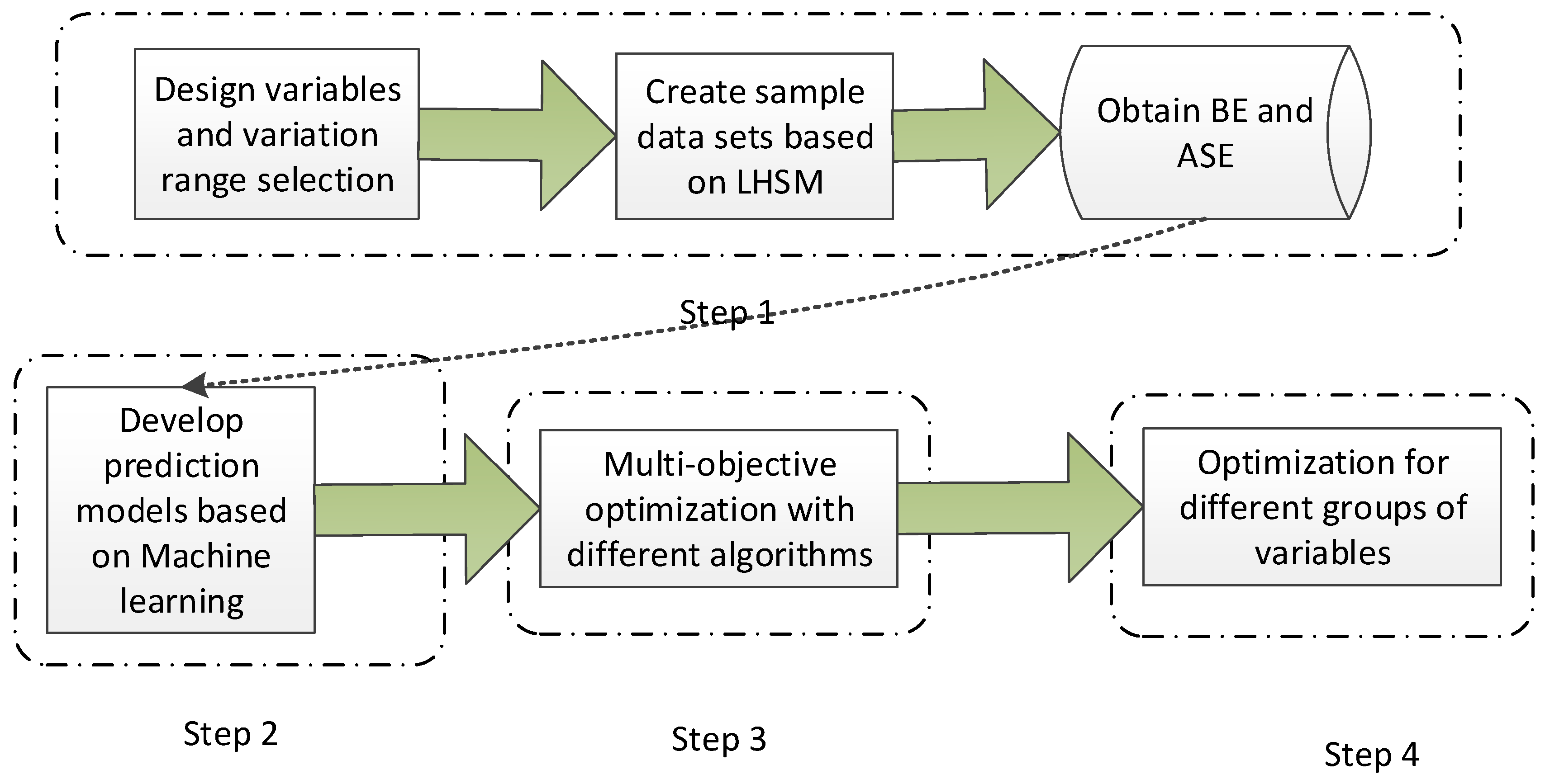
A total of 35 design parameters were considered, which took into account the green roof physical properties, building shape, building envelope properties, and air-conditioning thermostat settings. The optimization process comprised four steps (Figure 1). First, LHSM was used to generate a total of 800 sample buildings. Second, the sample buildings were simulated under the DesignBuilder environment [33], and associated building energy consumptions and visual discomfort levels were obtained. Third, a total of four machine learning approaches, including SLR, SVM, RF, and BPNN, were applied to develop prediction models for building energy consumption and visual comfort. The approaches with the best prediction performance were selected and coupled with six optimization algorithms, including three evolutionary algorithms and three group intelligence algorithms, for design optimization. Finally, the design variables were divided into four groups and the impact of different groups of design variable combinations were evaluated. The DesignBuilder optimization module can only handle up to 10 design variables and 2 objectives [33], and therefore it was not adopted in this study.
3.1. Objective Functions
The optimization problem can be described as below:
where f1 is the per unit annual energy consumption of the building, f2 refers to visual discomfort, which is the percentage area not meeting the annual sun exposure (ASE) requirement (ASE not in range).
f1 is determined by the following equation:
where Q is the annual building energy consumption, which includes heating, cooling, lighting, and equipment energy consumption, which was obtained by DesignBuilder [33], in kW; s is the building construction area, in m2.
The ASE is used as the indicator for daylight analysis. The ASE requirement from LEED [34] requests that not more than 10% of the space have a lighting intensity of over 1000 lux for a maximum of 250 h per year. Mangkuto et al. [35] utilized ASE as a performance indicator for internal shading device optimization.
f2 (ASE not in range) can then be calculated as:
where ASE250 is the is the area where lighting intensity is over 1000 lux for over 250 h per year.
ASE250 can be calculated by:
where ASEDB is the area of space satisfying the annual sunlight exposure (ASE) requirements, as calculated by DesignBuilder [33].
3.2. Building Model and Design Parameter Setting
The building investigated is located in Shanghai, which has a subtropical monsoon climate with four distinct seasons, abundant sunshine, and abundant rainfall. The climate is mild and humid, with a short spring and autumn, and long winter and summer. The annual average temperature in Shanghai is 16.2 °C with a heating degree day (HDD 18) of 1540 °C⋅d and cooling degree day (CDD 26) of 199 °C⋅d [36].
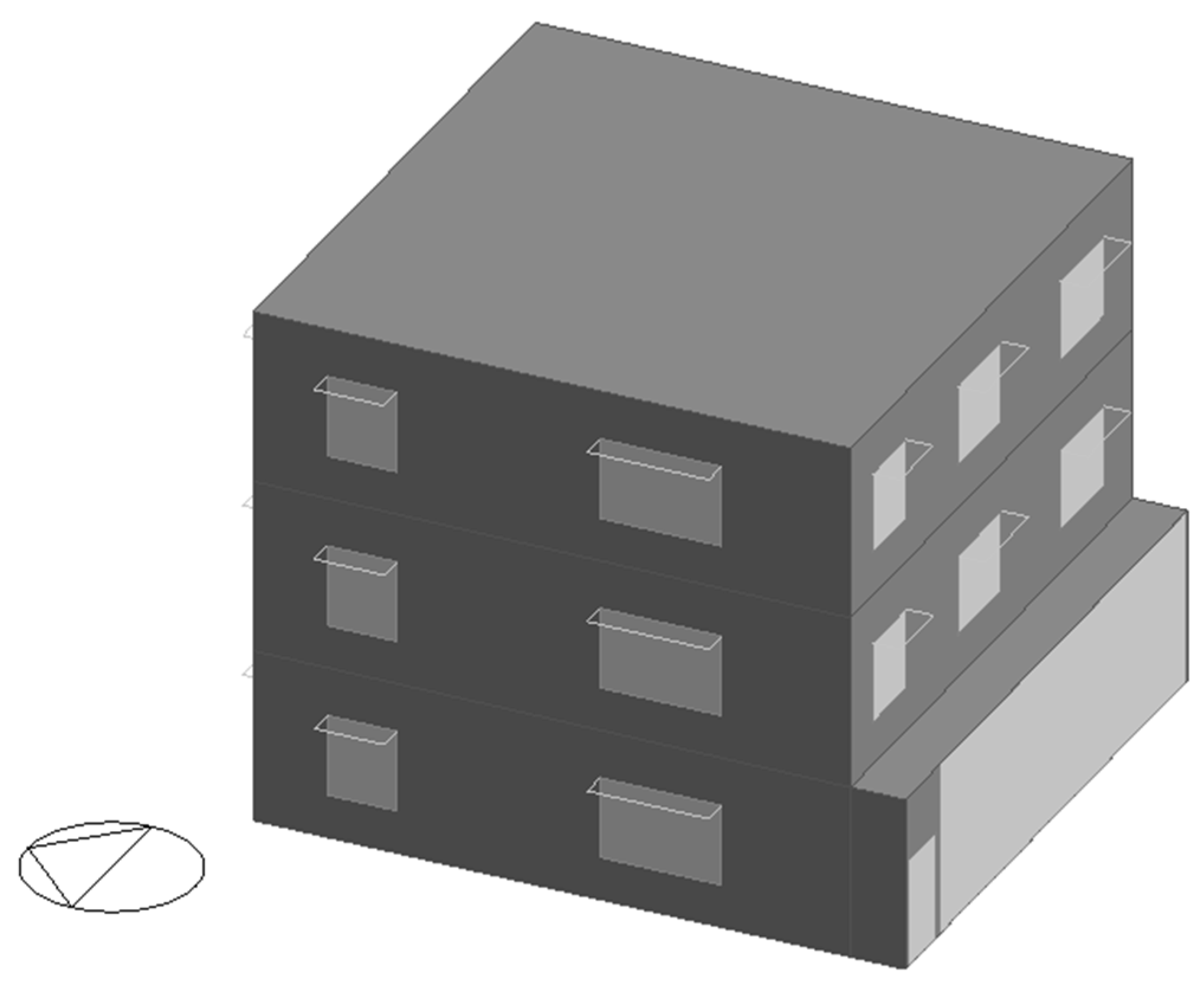
The floor area of each story is 120 m2 with a height of 3.2 m. It is a reinforced concrete frame structure building. Figure 2 presents the front view of a reference building with overhang shading. A door with a dimension of 1.5 m × 2.1 m is open to the south. The building orientation is due south, with a sunroom attached on the first floor. The heating seasonal and heating seasonal coefficients of performance (COPs) of the air-conditioning unit were set to be 2.3 and 1.9, respectively, according to [37]. A typical residential occupancy pattern was assigned. The fresh air rate was 30 m3/h per capita and ACH was 0.6. The lighting density, equipment load, and humidity generation were set to be 5 W/m2, 4 W/m2, and 100 g/(p⋅h), respectively, according to [38]. The occupant density and activity levels are listed in Table 2.
Table 3 presents the design parameters and their associated value ranges, which were selected and modified after careful consideration based on the references listed in Table 3. There are two types of parameters. The first type are discrete parameters (as shown in Table 4), which include floor number, length to width ratio, and window type. The second type are continuous parameters, which include the rest of the parameters.
The annual energy consumption and ASE area not in range for the reference building were 11,262.55 kWh (31.28 kWh/m2) and 8.9%, respectively.
3.3. Optimization Procedure
The optimization procedure included four steps (see Figure 1). First, a total of 800 samples were created based on LHSM, and the associated annual building energy consumption and ASE area in range were calculated using DesignBuilder [33]. Second, a total of four machine learning approaches were applied to develop the prediction models based on the simulation outcomes and associated values of the design parameters. The machine learning prediction models with the best prediction performance were selected for the subsequent analysis. Third, a total of six different optimization algorithms were coupled with the selected prediction models, searching through the 35-dimensional space, with value ranges provided in Table 3 and Table 4, to find the optimal solutions (with minimal energy consumption and maximum visual comfort), and the ones with the best performance were selected. Fourth, the selected optimization algorithm and prediction models were coupled to find the optimal solution for different combinations of design parameters to analyze the impact of design parameters in various aspects.
4. Prediction Model
4.1. Design Sample Creation
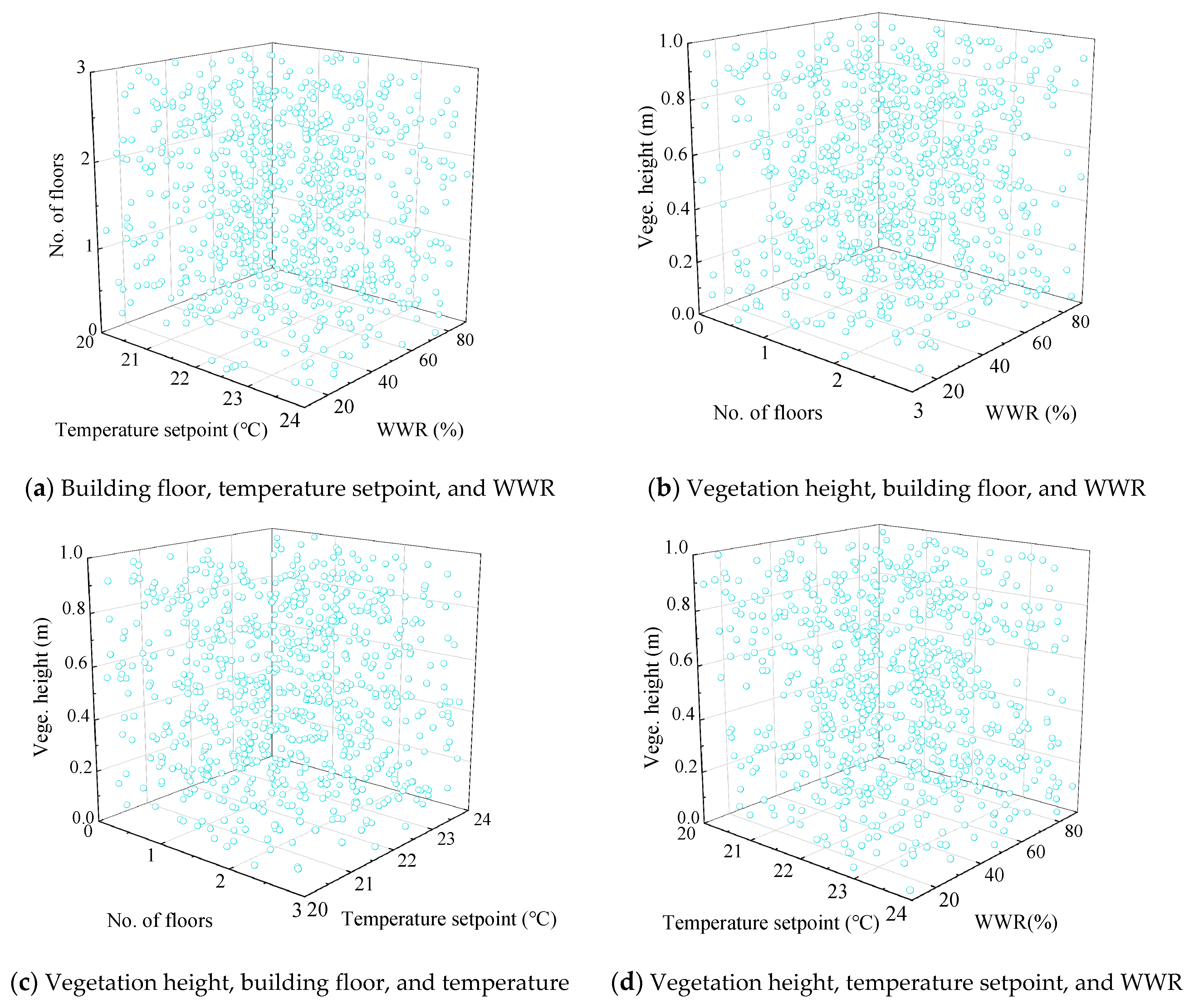
LHSM was proposed by McKay [39], and can ensure sampling variables are evenly distributed in a variable space. In addition, excluding certain dimensions of data from the sampling results will not affect their completeness [40], and therefore the impact of a certain group of variables can be investigated without the need for re-sampling.
The number of samples in this study was 800, with 35 design parameters, and following the principle of N ≥ 2 2.5 × M (M is the number of design parameters) from [6,41]. The variables could be divided into four groups related to building shape, air-conditioning settings, building envelope properties, and green roof configurations. Visualizations of the selected design parameters are presented in Figure 3.
4.2. Prediction Model through Machine Learning
Four learning approaches, including stepwise regression, BPNN, SVM, and RF, were used to develop the prediction models. The best prediction models were selected to carry out the optimization. A detailed analysis of the four machine learning approaches is described as follows.
4.2.1. SLR
SLR solves the problem of multiple linear relationships between variables and finds the optimal subset for regression. It makes a univariate regression between the dependent variable and each independent variable, and the independent variables are sequentially introduced after being sorted by importance. At the same time, F-test is conducted for the introduced variable, and those that are not of significance in the equation are eliminated. Finally, all the significant regression variables are included in the regression model as below:
where β0 is the regression constant and βi are the regression coefficients.
In this study, logarithmic SLR was adopted to develop the prediction model for the building energy consumption as below:
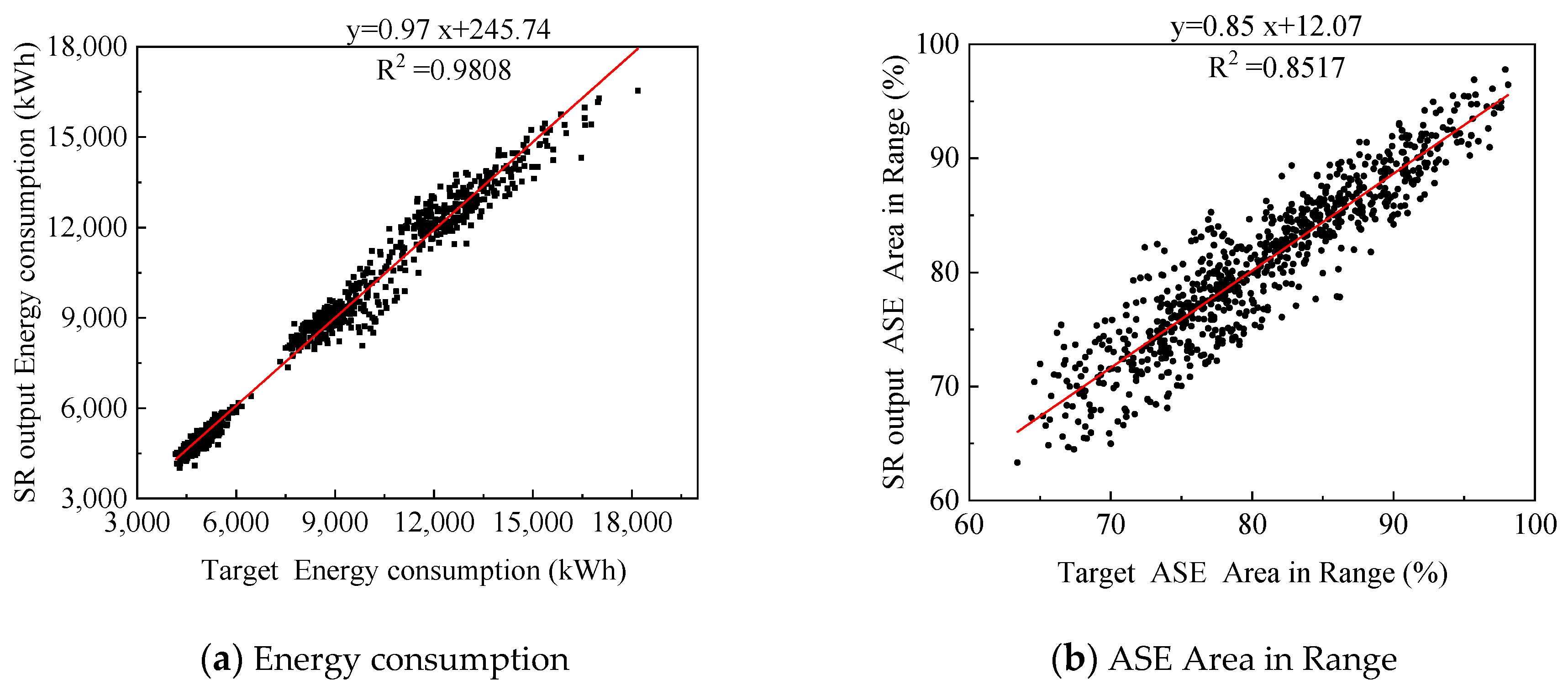
The outcomes of the regression models for the building energy consumption and ASE in range are presented as Equations (6) and (7):
The regression between the target simulation outputs and the prediction results is shown in Figure 4. It can be seen that the simulation results are in good agreement with the prediction results, with regression coefficients higher than 0.8517.
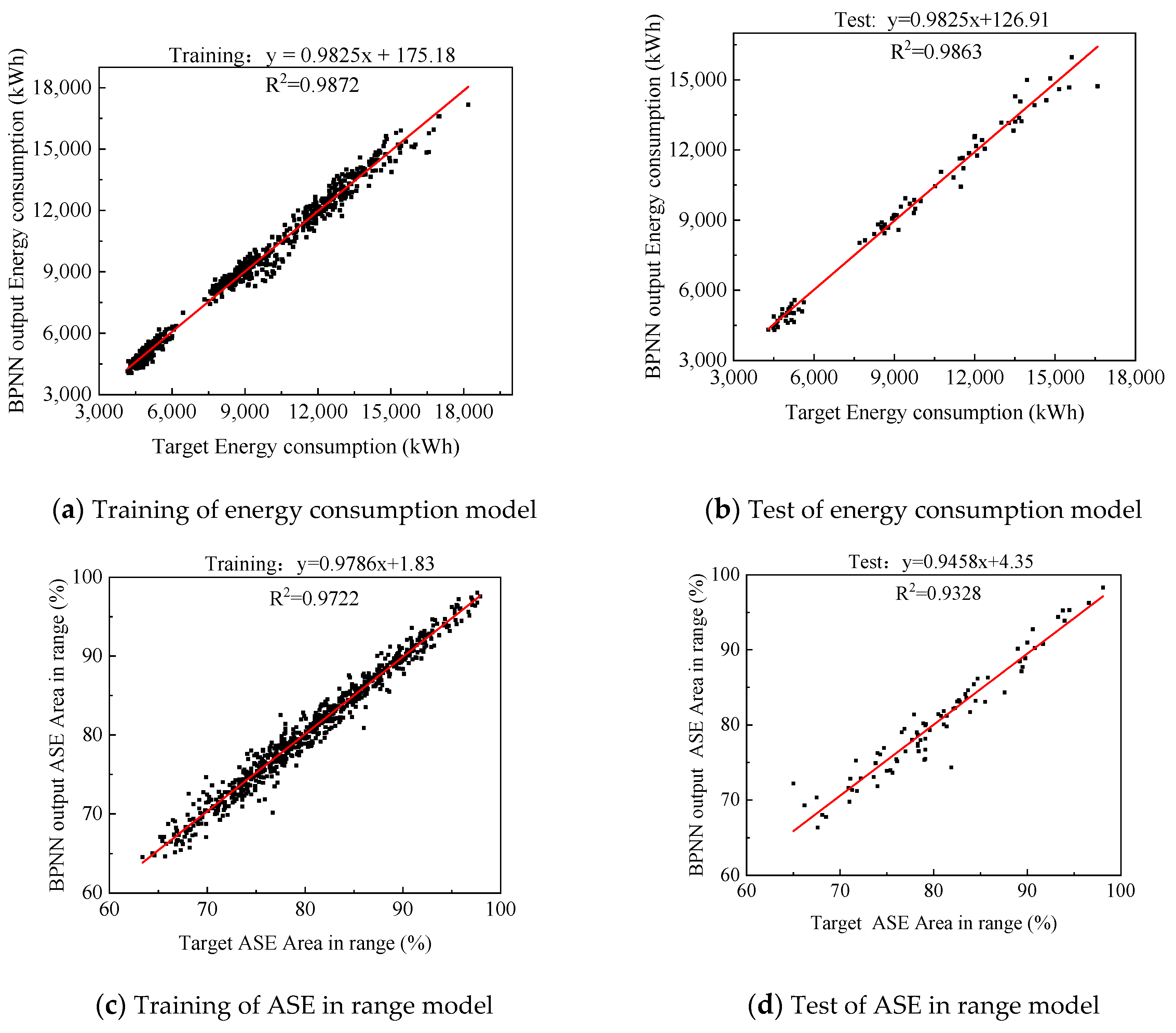
4.2.2. BPNN
BPNN is the most widely used type of neural network, includes input, hidden, and output layers, and can better solve various problems in practical applications. The hidden layer contains all the information processing and calculation processes, and can have one or more layers. Based on the empirical formula and testing, the final number of neurons for each layer are determined and listed in Table 5.
The Levengerg–Marquardt method was applied for training. The percentages of data used for training and validation were 90% and 10%, which were recommended by Zhang et al. [42] and Lu et al. [43]. The regression between the target simulation outputs and the prediction results is shown in Figure 5. Good agreements are found with the R-squares higher than 0.93.
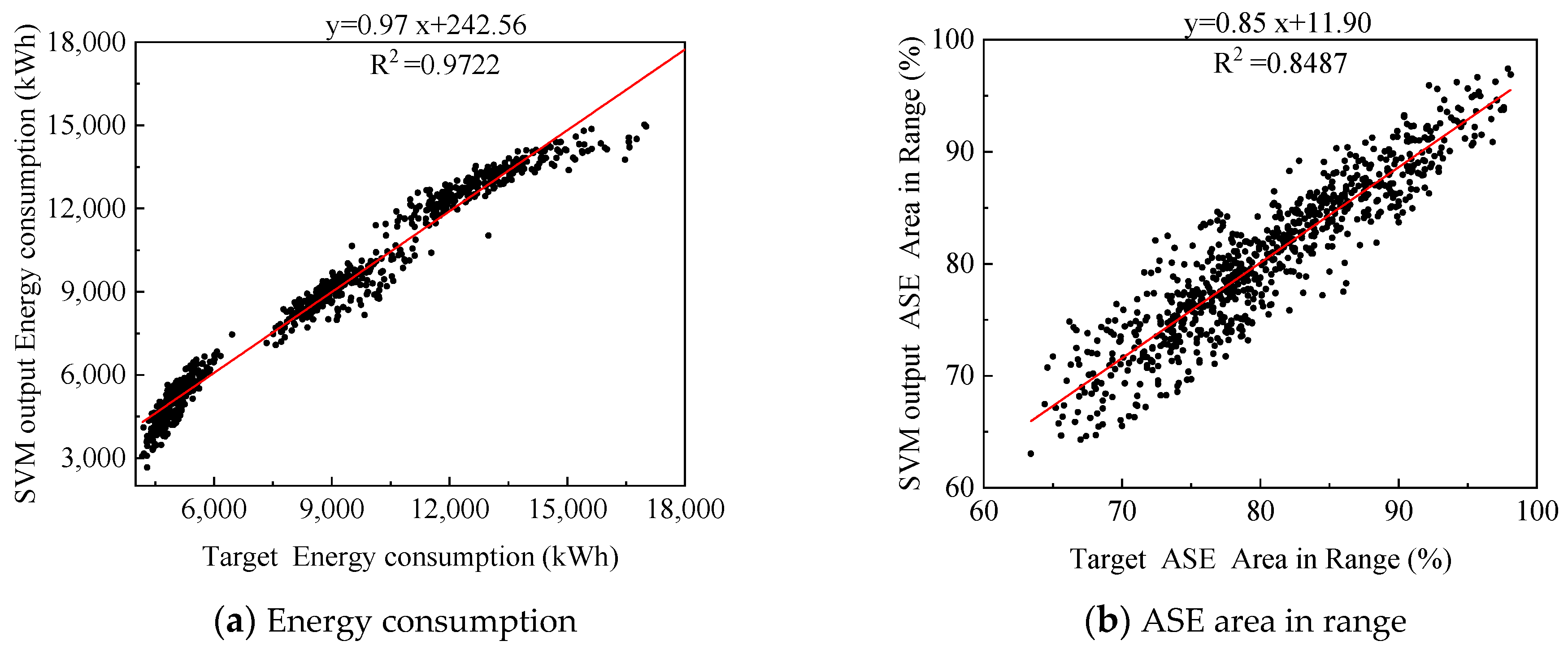
4.2.3. SVM
SVM has been widely used to solve practical problems. It is based on statistical learning and introduces the principle of structural risk minimization, which effectively solves the problem of dimensionality difficulties and local minima [44]. Support vector regression (SVR) is a type of SVM, which studies the relationship between output parameters and input parameters, and predicts the output variable values of new samples with the same distribution as the training sample set. The specific step is to introduce a loss function for distance correction under the premise of classification, thereby determining the regression model for prediction [45]. The regression between the target simulation outputs and the prediction results is shown in Figure 6. Good agreements are found with the R-squares higher than 0.85.
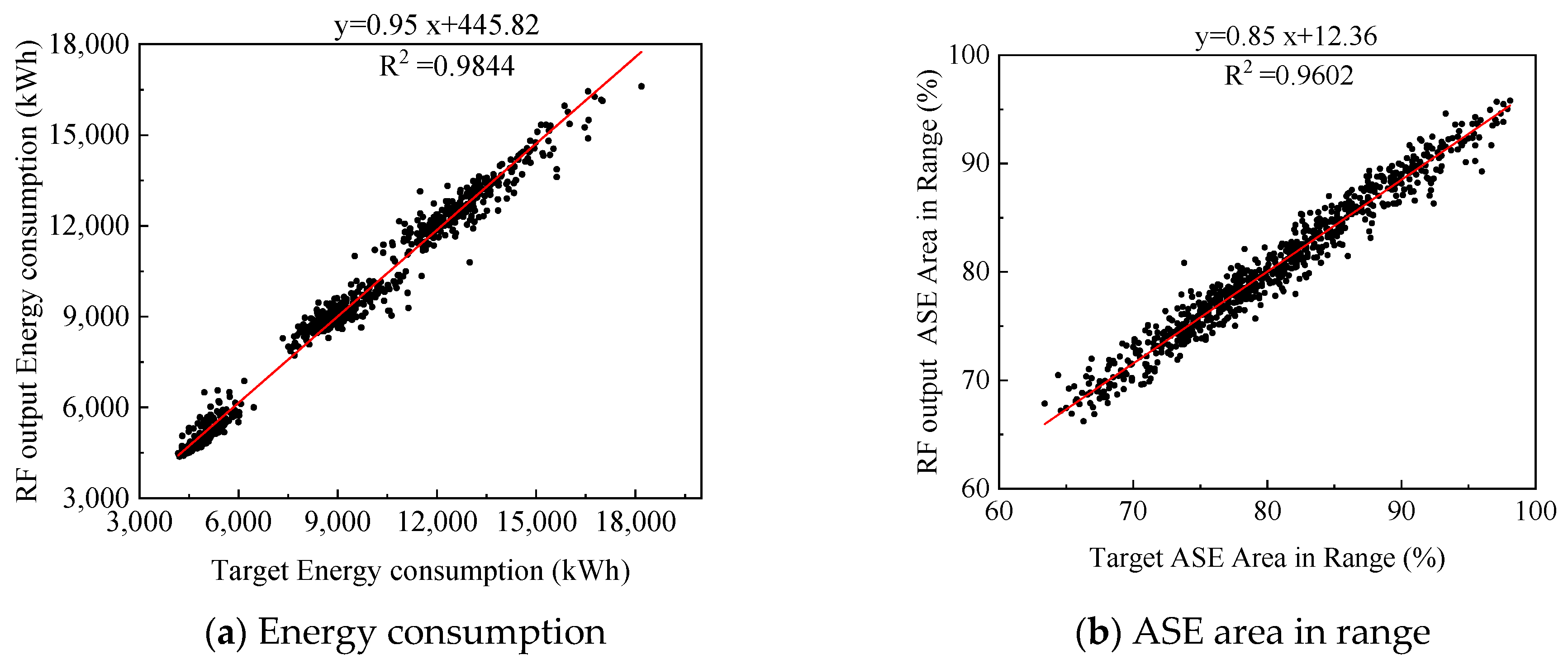
4.2.4. RF
RF is a further combination of classification trees, which improves the accuracy of the results without significantly increasing the amount of calculation. RF is not sensitive to multi-collinearity, and the outputs are relatively stable for missing and unbalanced data and make good use of as much independent variable information as possible [46]. Compared with traditional decision trees, RFs have a stronger fault tolerance. The regression between the target simulation outputs and the prediction results is shown in Figure 7. Good agreements are found with the R-squares higher than 0.96.
4.3. Comparisons on the Prediction Models
The outcomes of the relative error ranges for each model are listed in Table 6. It can be observed that the relative error of the visual comfort model was slightly lower than that of the energy consumption model. This may be due to the fact that the visual comfort was affected by fewer design parameters, and therefore, with the same amount of training, its prediction accuracy was higher than that of the energy consumption. Table 6 also points out that the BPNN model had the best prediction performance, with an average relative error of 3.27% and 1.25% for energy consumption and ASE area in range, respectively. The SVM model had a slightly higher average relative error for both energy consumption and ASE area in range compared with the other prediction models.
Table 7 presents the R-squares of each model, which also shows that the BPNN model had the highest R-square, followed by RF, SLR, and SVM. In particular, for the prediction of ASE area in range, the BPNN model significantly outperformed the other models.
Based on the above results, the BPNN models were selected to couple with the optimization algorithms to carry out the design optimization in this study. The BPNN is flexible for nonlinear modeling, and has strong adaptability, learning, and massive parallel computing abilities.
5. Optimization
Two types of optimization algorithm, the evolutionary algorithm and group intelligence algorithm, were applied in this study, and are discussed in the following sections.
5.1. Evolutionary Algorithm
The evolutionary algorithm (EA) [47] is a random search algorithm that imitates biological evolution. It can handle complex nonlinear problems well and is widely used in solving practical optimization problems. It has a good versatility for multi-objective optimization problems. In this study, three algorithms, i.e., multi-objective evolutionary algorithm based on decomposition (MOEA/D), non-dominated sorting genetic algorithm –II (NSGA-II), and non-dominated sorting genetic algorithm –III (NSGA-III) were used for design optimization.
5.1.1. MOEA/D
MOEA/D is an evolutionary algorithm based on decomposition, through which a multi-objective optimization problem is decomposed into a set of multiple single-objective optimization problems with different weighting factors to approach the Pareto front [48]. In this study, the Tchebycheff aggregate function method was used to assign weight vectors to each sub-problem.
5.1.2. NSGA-II
The NSGA-II algorithm by Deb was improved on the basis of the non-dominated sorting genetic algorithm, and introduces a fast non-dominated genetic algorithm with an elite strategy and a crowding degree comparison operator, which can not only reduce the computational complexity but also obtain a more evenly distributed Pareto optimal solution [49]. The NSGA-II algorithm has a faster convergence speed and a better Pareto solution set. It has become the performance benchmark for many other multi-objective optimization algorithms and is widely used in solving multi-objective optimization problems.
The parameters settings of the NSGA-II algorithm were as follows: population size D = 40; crossover probability Pc = 0.99; mutation probability Pm = 0.0001; termination evolution algebra G = 200.
5.1.3. NSGA-III
NSGA-III is a third-generation non-dominated sorting genetic algorithm proposed on the basis of the NSGA-II algorithm, and with improvement to the selection mechanism to allow more uniform population distribution and more abundant individual diversity [50]. The NSGA-III algorithm has the same calculation steps as the NSGA-II algorithm, but its individual selection mechanism is based on reference points [50].
The basic settings of the NSGA-III algorithm were as follows: population size D = 50; maximum generation for iteration G = 80.
5.2. Group Intelligence Algorithm
The group intelligence algorithm is a new method for solving problems based on the social group behavior of certain animals and the inherent principles of artificial life theory. In this study, the traditional multi-objective particle swarm algorithm (MOPSO) and the relatively new, but more widely used, multi-objective dragonfly algorithm (MODA) and multi-objective ant lion optimization algorithm (MOALO) were used.
5.2.1. MOPSO
The MOPSO algorithm imitates group social behaviors by using particles to search for the most feasible area in the solution space [51]. Each particle represents a certain search position in the solution space and with a searching speed, combined with the fitness function to adjust the position, the algorithm finally determines the particle′s flight direction towards the optimal solutions.
5.2.2. MODA
The dragonfly algorithm (DA) imitates the social behavior of dragonfly groups [52]. A total of five behavior parameters, including separation, formation, gathering, predation, and escape, are used to imitate dragonfly behavior and update the position of each individual in the group.
5.2.3. MOALO
The MOALO algorithm imitates the foraging behavior of antlions in nature and has a better global search ability than particle swarm and genetic algorithms [53]. The antlion algorithm gradually finds the approximate optimal solution by exploring random solutions. Unlike the traditional swarm intelligence optimization algorithm, there are two opposing species in the ant lion optimization (ALO) algorithm: ants and antlions. Six basic steps of antlion predation processes are imitated, which include: (1) ants move randomly; (2) antlions build traps; (3) ants fall into traps; (4) ants slides towards antlions; (5) antlions capture ants; and (6) antlions rebuild traps [54].
5.3. Comparison of Optimization Algorithms
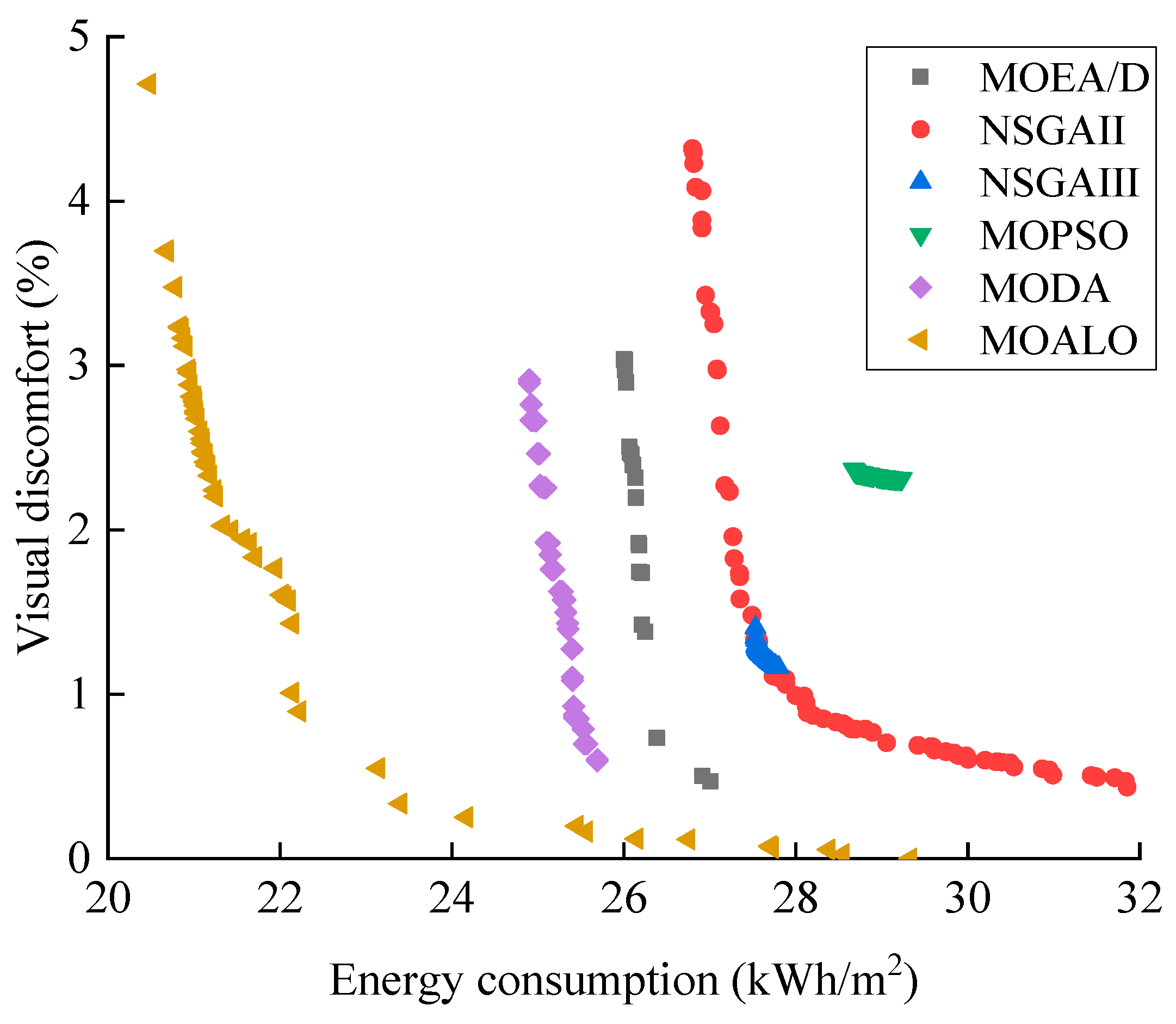
Figure 8 presents a comparison of the outcomes of the Pareto solutions from different optimization algorithms. It can be observed that the MOALO algorithm led to the best Pareto front, which means its performance was the best. The MOPSO algorithm appeared to have the worst performance among the six optimization algorithms. Among the evolutionary algorithms, MOEA/D had the best performance, and NSGA-III only obtained parts of the optimal solutions compared with NSGA-II. Excepting MOPSO, the other two group intelligence algorithms (MODA and MOALO) outperformed all of the three evolutionary algorithms. However, the running times of the group intelligence algorithms were about three to four times that of the evolutionary algorithms.
Comparisons of the ranges of visual discomfort, energy consumption, number of optimal solutions, and running time for the different optimization methods are listed in Table 8. It can be noted that the visual discomforts were all less than 5%, and the energy consumptions (except the ones from NSGA-II) were all less than 29.3 kWh/m2. Compared with the reference building energy consumption of 31.28 kWh/m2 and visual discomfort of 8.9%, the improvements to the building’s thermal and visual performance were remarkable for all the optimal solutions.
A further data analysis was conducted for the MOALO algorithm, with 100 optimal solutions. Table 9 presents the ranges of the design parameters recommended based on the optimal solutions provided by the MOALO algorithm. It shows that the design of passive houses in hot summer and cold winter areas should focus on heat insulation design. As is obvious, the WWR for the east, west, and south facades should be kept at 10%, and no window should be provided on the north facade. Triple-layer Low-E glazing and a plant height of 0.2–0.5 m are also recommended based on the optimal solutions. A floor number of 3 is recommended, meaning the most compact building shape is preferred. A cooling temperature setpoint of 24–26 °C and heating temperature setpoint of 20–22 °C are recommended, which differ from the recommended values from the design standard [30], of 26 °C and 18 °C, respectively. Moreover, it can be noticed that the recommended value ranges for the overhang length, absorptance of solar radiation, concrete thickness, and insulation thickness for different parts of the building differ, which means that the building envelopes can be customized to achieve optimal performance. This is different from traditional building design approach that has uniform envelope properties. The above design strategies are consistent with the ones recommended by Climate Consultant software [55], which also proposes low-E glazing, window overhangs, compact building size, high level insulation, thermal mass, raising thermal-stat setpoint, and using plant materials in Shanghai.
5.4. Group Optimization
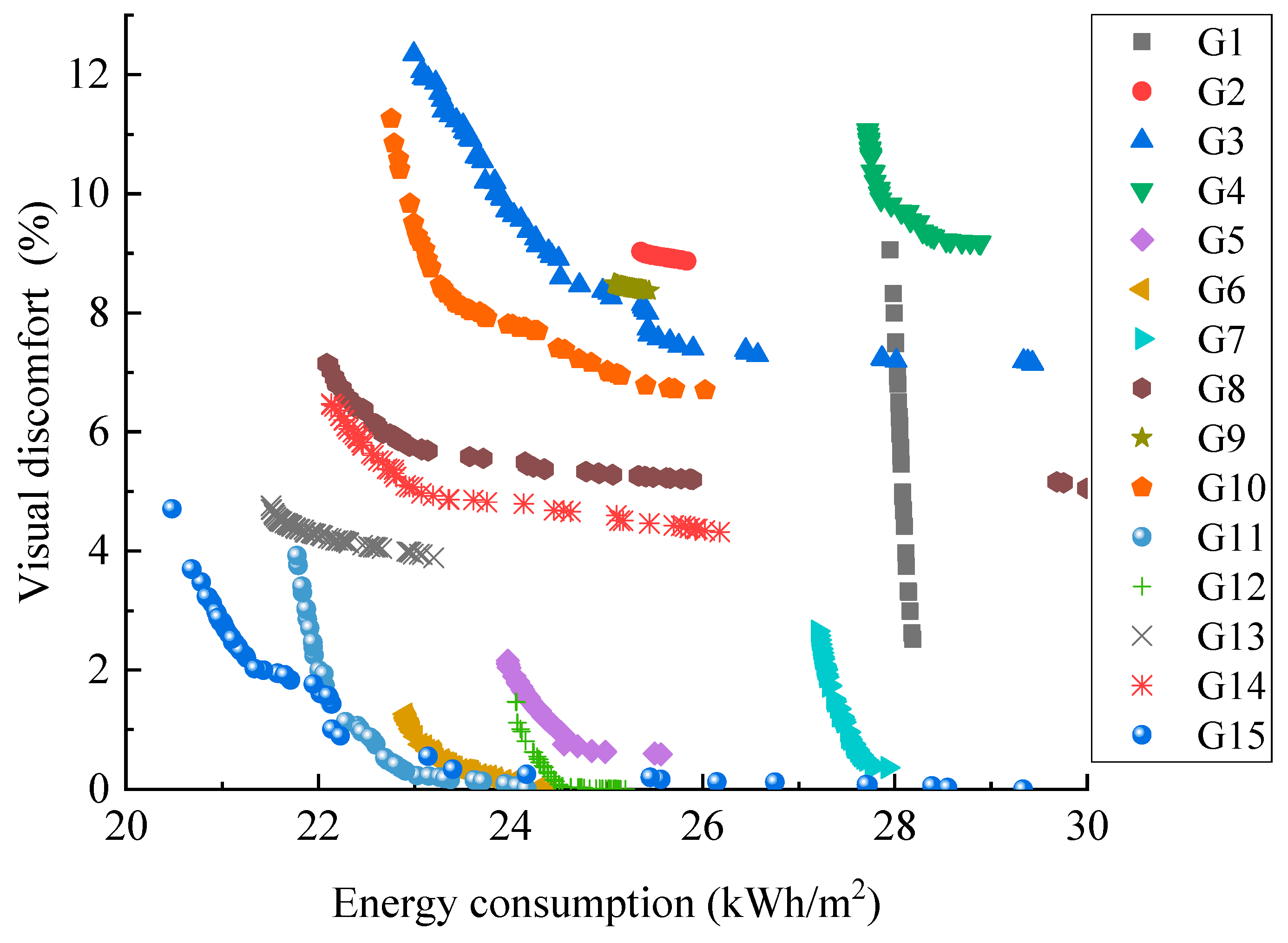
In order to evaluate the influence of various building parameters on the performance of the building, the 35 parameters were divided into groups, which were related to building shape (G1, including x1,x2, and x29), air conditioning system (G2, including x3,x4, and x35), physical properties of the building envelope (G3, including x5–x28), and green roof (G4, including x30–x34). A total of 15 different combinations can be formed. Figure 9 presents a comparison of the Pareto fronts for the 15 combinations. It can be observed that G15 has the best Pareto front and G4 has the worst Pareto front. This result indicates that as the number of design parameters increases, the Pareto front becomes lower. Therefore, the inclusion of more design parameters in the optimization process can lead to better optimal solutions.
Table 10 lists the ranges and average values of energy consumption and visual discomfort for different groups of combinations. For energy consumption, the optimization of the air-conditioning (G2) and building physical property (G3) related parameters resulted in much lower values compared to the optimization of the green roof (G4) and building shape (G1). However, for visual comfort, building shape (G1) appeared to have the highest impact on visual comfort. Compared with the reference building, the optimization of G15 leads to 29.96% energy consumption reduction and 71.80% visual discomfort improvement on average. The inclusion of a green roof (G4) led to an average reduction of 9.88% on the energy consumption but had no impact on the indoor visual comfort.
6. Conclusions
In this paper, a passive building with a green roof located in Shanghai in the hot summer and cold winter region of China, was optimized by taking the building energy consumption and visual discomfort as the objectives. A total of 35 design parameters related to building shape, building envelope properties, air-conditioning system settings and green roof configurations were considered. Four machine learning approaches were used to develop prediction models for building energy consumption and visual comfort, and six optimization algorithms were evaluated to find the optimal design solutions. The following conclusions can be made:
- (1)
- Among the four machine learning prediction models, the BPNN models had the best performance in predicting both building energy consumption and visual comfort, with R-squares of 0.987 and 0.966, respectively.
- (2)
- The evolutionary algorithms converged faster than the group intelligent algorithms. However, the group intelligent algorithms led to lower Pareto front solutions. The MOALO algorithm coupled with BPNN prediction models had the best performance, resulting in a 29.96% energy consumption reduction and 71.80% visual discomfort improvement on average.
- (3)
- The thermal performance of a building can be improved by involving more design parameters in the optimization process. The building envelope physical properties and air conditioning system setpoints have a greater impact on building energy consumption, and the building shape related design parameters have a greater impact on the visual discomfort.
- (4)
- The inclusion of a green roof lead to an average reduction of 9.88% in the energy consumption (28.19 kWh vs. 31.28 kWh). However, its impact on the indoor visual comfort is minimal. Meanwhile, the recommended value ranges for the overhang length, absorptance of solar radiation, concrete thickness, and insulation thickness for different parts of the building were not uniform, which means that the building envelopes can be customized for 3-D printing.
The outcomes of this study could help architects and building design engineers during the design process, for the optimization of visual comfort and energy consumption. The optimal design solutions can provide a more comfortable living environment to improve the occupants’ productivity and well-being, and yet have less energy consumption, which would be a selling point for investors when considering the construction of passive buildings. Difficulties that may be encountered by the users of the proposed methods and algorithms coud the need to use the design parameters in the recommended ranges, together with the prediction model for accurate prediction of the thermal and visual performance of buildings. However, this could be overcome by embedding the prediction model into a spreadsheet for quick calculation.
Author Contributions
Y.L. and W.Y. contributed to the conception of the study, the development of the methodology. L.Z. and Y.L. developed computer models, and simulated and analyzed data. Y.L. and W.Y. contributed to the whole revision process. Y.L., L.Z., X.L., W.Y., X.H. and L.T. wrote the manuscript. All authors have read and agreed to the published version of the manuscript.
Funding
This research was funded by Natural Science Foundation of Hubei Province, grant number [2017CFB602] and Hunan Provincial Department of housing and urban rural development, grant number [KY2016063].
Institutional Review Board Statement
Not applicable.
Informed Consent Statement
Not applicable.
Data Availability Statement
Acknowledgments
The authors acknowledge the support from School of Environment and Architecture, University of Shanghai for Science and Technology in China.
Conflicts of Interest
The authors declare no conflict of interest.
Abbreviations
| List of Acronyms | |
| ACH | Air Change rate per Hour |
| ALO | Ant Lion Optimization |
| ASE | Annual Sunlight Exposure |
| BPNN | Back-Propagation Neural Networks |
| CDD 26 | Cooling Degree Day indoor setpoint temperature of 26℃ |
| CFD | Computational Fluid Dynamics |
| COP | Coefficient Of Performance |
| DA | Dragonfly Algorithm |
| EA | Evolutionary algorithm |
| HDD 18 | Heating Degree Day with indoor setpoint temperature of 18℃ |
| lr | Leaf reflectivity |
| LAI | Leaf area index |
| LHSM | Latin Hypercube Sampling Method |
| MOALO | Multi-Objective Ant Lion Optimization |
| MOALO | Multi-Objective Ant Lion Optimization Algorithm |
| MODA | Multi-Objective Dragonfly Algorithm |
| MOEA/D | Multi-objective Evolutionary Algorithm Based on Decomposition |
| MOPSO | Multi-Objective Particle Swarm Algorithm |
| NSGA-II | Non-dominated Sorting Genetic Algorithm -II |
| NSGA-III | Non-dominated Sorting Genetic Algorithm -III |
| RF | Random Forest |
| SHGC | Solar Heat Gain Coefficient |
| SLR | Step Linear Regression |
| SVM | Support Vector Machine |
| SVR | Support Vector Regression |
| WWR | Window-to-Wall Ratio |
References
- Gong, X.; Akashi, Y.; Sumiyoshi, D. Optimization of passive design measures for residential buildings in different Chinese areas. Build. Environ. 2012, 58, 46–57. [Google Scholar] [CrossRef]
- Wu, D.; Liu, L.; Li, X.; Liu, C. Research on the Technologies of Passive Low Energy Buildings on the Basis of Multi-Objective Optimization Method-by Taking Cold Zone Residential Buildings for Example. J. Cent. South Univ. (Nat. Sci. Ed.) 2018, 46, 98–104. [Google Scholar]
- Pang, H. Passive Design Strategies of Residential Building in the Severe Cold Mountains Regions. Master’s Thesis, Harbin Institute of Technology, Harbin, China, 2016. [Google Scholar]
- Ralegaonkar, R.V.; Gupta, R. Review of intelligent building construction: A passive solar architecture approach. Renew. Sustain. Energy Rev. 2010, 14, 2238–2242. [Google Scholar] [CrossRef]
- Lin, Y.; Yang, W. Application of Multi-Objective Genetic Algorithm Based Simulation for Cost-Effective Building Energy Efficiency Design and Thermal Comfort Improvement. Front. Energy Res. 2018, 6, 25. [Google Scholar] [CrossRef] [Green Version]
- Lin, Y.; Zhou, S.; Yang, W.; Li, C.Q. Design Optimization Considering Variable Thermal Mass, Insulation, Absorptance of Solar Radiation, and Glazing Ratio Using a Prediction Model and Genetic Algorithm. Sustainability 2018, 10, 336. [Google Scholar] [CrossRef] [Green Version]
- Dodoo, A.; Gustavsson, L.; Sathre, R. Lifecycle primary energy analysis of conventional and passive houses. Int. J. Sustain. Build. Technol. Urban Dev. 2012, 3, 105–111. [Google Scholar] [CrossRef]
- Asadi, E.; da Silva, M.G.; Antunes, C.H.; Dias, L. A multi-objective optimization model for building retrofit strategies using TRNSYS simulations, GenOpt and MATLAB. Build. Environ. 2012, 56, 370–378. [Google Scholar] [CrossRef]
- Flaga-Maryanczyk, A.; Schnotale, J.; Radon, J.; Was, K. Experimental measurements and CFD simulation of a ground source heat exchanger operating at a cold climate for a passive house ventilation system. Energy Build. 2014, 68, 562–570. [Google Scholar] [CrossRef]
- He, Y.; Yu, H.; Ozaki, A.; Dong, N.; Zheng, S. Long-term thermal performance evaluation of green roof system based on two new indexes: A case study in Shanghai area. Build. Environ. 2017, 120, 13–28. [Google Scholar] [CrossRef]
- Olivieri, F.; Perna, C.D.; D’Orazio, M.; Olivieri, L.; Neila, J. Experimental measurements and numerical model for the summer performance assessment of extensive green roofs in a Mediterranean coastal climate. Energy Build. 2013, 63, 1–14. [Google Scholar] [CrossRef]
- Zou, F.; Song, K.; Guo, E.; Li, Y. Researches on Indicators of Passive Ultra-low energy Buildings in Tianjin. Build. Sci. 2018, 34, 49–55. [Google Scholar]
- Feng, Y.; Yang, X.; Zhong, H. Heating Potential of Passive Solar Building in Lhasa. HV&AC. 2013, 43, 31–34. [Google Scholar]
- Li, E.; Yang, L.; Liu, J. Analysis on the passive design optimization for residential buildings in Lhasa based on the case study of attached sunroom system for apartment buildings. J. Xi’an Univ. Arch. Technol. (Nat. Sci. Ed.) 2016, 48, 258–264. [Google Scholar]
- Zhang, Z. Application Research of Passive House Techniques on Rurual Houses in Southern Regions of Jiangsu Province. Master’s Thesis, Southeast University, Nanjing, China, 2016. [Google Scholar]
- Fu, Y. Study on Passive Regulation Strategy of Indoor Thermal Environment of Stone Houses in Cold Area of Sichuan. Master’s Thesis, Southwest University of Science and Technology, Mianyang, China, 2019. [Google Scholar]
- Chen, X.; Yang, H.; Wang, Y. Parametric study of passive design strategies for high-rise residential buildings in hot and humid climates: Miscellaneous impact factors. Renew. Sustain. Energy Rev. 2017, 69, 442–460. [Google Scholar] [CrossRef]
- Zhang, L.; Bai, X.; Zhu, Z. Application effect of passive technologies under different climate conditions in the Yangtze river basin. HV&AC 2018, 48, 54–60. [Google Scholar]
- Song, X.; Yang, J.; Hang, W. Research on the economy optimization of passive solar building. Acta Energ. Sol. Sin. 2012, 33, 1425–1429. [Google Scholar]
- Zhao, X.; Liu, P.; Zhu, Z.; Sang, G. Rurual residence passive design strategiesin Southern Shananxi basedon improving thermal comfort. J. Xi’an Univ. Technol. 2014, 30, 315–319. [Google Scholar]
- Yang, L. Climatic Analysis and Architectural Design Strategies for Bio-Climatic Design. Ph.D. Thesis, Xi’an University of Architecture and Technology, Xi’an, China, 2003. [Google Scholar]
- Hui, X. Exploring the Design of Passive Energy Saving Building Based on the BIM Technology. Master’s Thesis, Anhui Jianzhu University, Hefei, China, 2017. [Google Scholar]
- Chandel, S.S.; Sarkar, A. Performance assessment of a passive solar building for thermal comfort and energy saving in a hilly terrain of India. Energy Build. 2015, 86, 873–885. [Google Scholar] [CrossRef]
- Sharifi, A.; Yamagata, Y. Roof ponds as passive heating and cooling systems: A systematic review. Appl. Energy 2015, 160, 336–357. [Google Scholar] [CrossRef]
- Zirnhelt, H.E.; Richman, R.C. The potential energy savings from residential passive solar design in Canada. Energy Build. 2015, 103, 224–237. [Google Scholar] [CrossRef]
- Morrissey, J.; Moore, T.; Horne, R.E. Affordable passive solar design in a temperate climate: An experiment in residential building orientation. Renew. Energy 2010, 36, 568–577. [Google Scholar] [CrossRef]
- Triantafyllidou, E.F.; Michael, A.G. The impact of installing a concave curved profile blind to a glass window for visual comfort in office buildings. Procedia Manuf. 2020, 44, 269–276. [Google Scholar] [CrossRef]
- Andargie, M.S.; Touchie, M.; O’Brien, W. A review of factors affecting occupant comfort in multi-unit residential buildings. Build. Environ. 2019, 160, 106182. [Google Scholar] [CrossRef]
- Dounis, A.I.; Santamouris, M.J.; Lefas, C.C.; Manolakis, D.E. Thermal-comfort degradation by a visual comfort fuzzy-reasoning machine under natural ventilation. Appl. Energy 1994, 48, 115–130. [Google Scholar]
- Michael, A.; Gregoriou, S.; Kalogirou, S.A. Environmental assessment of an integrated adaptive system for the improvement of indoor visual comfort of existing buildings. Renew. Energy 2018, 115, 620–633. [Google Scholar] [CrossRef]
- Kim, M.; Konstantzos, I.; Tzempelikos, A. Real-time daylight glare control using a low-cost, window-mounted HDRI sensor. Build. Environ. 2020, 177, 106912. [Google Scholar] [CrossRef]
- ElBatran, R.M.; Ismaeel, W.S.E. Applying a parametric design approach for optimizing daylighting and visual comfort in office buildings. Ain Shams Eng. J. 2021, in press. [Google Scholar] [CrossRef]
- DesignBuilder Software Ltd. Available online: http://www.designbuilder.co.uk/ (accessed on 29 April 2020).
- USGBC. Available online: https://www.usgbc.org/leed/v41 (accessed on 6 January 2021).
- Mangkuto, R.A.; Dewi, D.K.; Herwandani, A.A.; Koerniawan, M.D.; Faridah. Design optimisation of internal shading device in multiple scenarios: Case study in Bandung, Indonesia. J. Build. Eng. 2019, 24, 100745. [Google Scholar] [CrossRef]
- Energy Plus. 2021. Available online: https://energyplus.net/ (accessed on 10 April 2021).
- MOHURD (Ministry of Housing and Urban-Rural Construction of the People’s Republic of China). Residential Building Energy Efficiency Design Standard for Hot Summer/Cold Winter Region; China Architectural Engineering Industrial Publishing Press: Beijing, China, 2010.
- MOHURD (Ministry of Housing and Urban-Rural Construction of the People’s Republic of China). Guideline for Passive Ultra-Low Energy Green Building Technology for Residential Buildings (Trial); China Architectural Engineering Industrial Publishing Press: Beijing, China, 2015.
- McKay, M.D.; Beckman, R.J.; Conover, W.J. Comparison of Three Methods for Selecting Values of Input Variables in the Analysis of Output from a Computer Code. Technometric 2000, 42, 55–61. [Google Scholar] [CrossRef]
- Fang, L. Research on Uncertainty Analysis Method Based on Latin Hypercube Sampling in the Probabilistic Safety Assessment. Master’s Thesis, University of Science and Technology of China, Hefei, China, 2015. [Google Scholar]
- Magnier, L.; Haghighat, F. Multiobjective optimization of building design using TRNSYS simulations, genetic algorithm, and Artificial Neural Network. Build. Environ. 2009, 45, 739–746. [Google Scholar] [CrossRef]
- Zhang, W.; Liu, F.; Fan, R. Improved thermal comfort modeling for smart buildings: A data analytics study. Int. J. Electr. Power Energy Syst. 2018, 103, 634–643. [Google Scholar] [CrossRef]
- Lu, S.; Wang, W.; Lin, C.; Hameen, E. Data-driven simulation of a thermal comfort-based temperature set-point control with ASHRAE RP884. Build. Environ. 2019, 156, 137–146. [Google Scholar] [CrossRef]
- Boser, B.; Guyon, I.; Vapnik, V. A training algorithmfor optimalmargin classifiers. In Proceedings of the 5th Annual ACM Workshop on Computational Learning Theory, Pittsburgh, PA, USA, 27–29 July 1992; Haussler, D., Ed.; Association for Computing Machinery: New York, NY, USA, 1992; pp. 144–152. [Google Scholar]
- Xue, W. SPSS Modeler Data Mining Approach and Application, 3rd ed.; Publish House of Electronic Industry: Beijing, China, 2020. [Google Scholar]
- Zhang, W. Advanced Lectures for SPSS Statistical Analysis; Higher Education Press: Beijing, China, 2017. [Google Scholar]
- Zheng, J. Multi-Objective Evolutionary Algorithms and Applications; Science Press: Beijing, China, 2017. [Google Scholar]
- Zhang, Q.; Li, H. MOEA/D: A Multi-objective Evolutionary Algorithm Based on Decomposition. IEEE Trans. Evol. Comput. 2007, 11, 712–731. [Google Scholar] [CrossRef]
- Deb, K.; Agrawal, S.; Pratap, A.; Meyarivan, T. A fast elitist non-dominated sorting genetic algorithm for multi-objective optimization: NSGA-II. In Proceedings of the 6th International Conference on Parallel Problem Solving from Nature, Paris, France, 18–20 September 2000. [Google Scholar]
- Deb, K.; Jain, H. An Evolutionary Many-Objective Optimization Algorithm Using Reference-Point-Based Nondominated Sorting Approach, Part I: Solving Problems With Box Constraints. IEEE Trans. Evol. Comput. 2014, 18, 577–601. [Google Scholar] [CrossRef]
- Carlos, A. A proposal for Multiple Objective Particle Swarm Optimization. In Proceedings of the 2002 Congress on Evolutionary Computation. CEC’02 (Cat. No.02TH8600), Honolulu, HI, USA, 12–17 May 2002; IEEE: Piscataway, NJ, USA, 2002; pp. 1051–1056. [Google Scholar]
- Jiao, L.; Gong, M.G.; Shang, R.; Du, H.; Lu, B. Clonal Selection with Immune Dominance and Anergy Based Multiobjective Optimization. In Proceedings of the International Conference on Evolutionary Multi-Criterion Optimization, Guanajuato, Mexico, 9–11 March 2005; Gong, M.G., Shang, R., Du, H., Eds.; Springer: Berlin/Heidelberg, Germany, 2005. [Google Scholar]
- Zitzler, E.; Künzli, S. Indicator-Based Selection in Multiobjective Search. In Proceedings of the International Conference on Parallel Problem Solving from Nature, Birmingham, UK, 18–22 September 2004; Springer: Berlin/Heidelberg, Germany, 2004. [Google Scholar]
- Li, H.; Lin, H.; Ding, Z. Virtual Machine Placement Algorithm Based on Multi-objective Ant Colony Optimization. Comput. Digit. Eng. 2018, 46, 2445–2449. [Google Scholar]
- Climate Consultant. 2021. Available online: http://www.energy-design-tools.aud.ucla.edu/ (accessed on 10 April 2021).
Figure 1.
Optimal solution procedure (BE: building energy consumption; ASE: ASE area in range).

Figure 2.
Front view of the reference building.

Figure 3.
Latin hypercube sampling results of selected design parameters.

Figure 4.
Stepwise regression model output and target fitting diagram.

Figure 5.
Neural network model output and target fitting diagram.

Figure 6.
SVM model output and target fitting diagram.

Figure 7.
RF model output and target fitting diagram.

Figure 8.
Pareto fronts for the different algorithms.

Figure 9.
Pareto fronts for different combinations of design parameters.


Table 1.
Design variables for passive buildings and green roof optimization from open literature.
| Location | Design Variable | Ref. |
|---|---|---|
| China | Window type, concrete thickness, insulation thickness, sunroom depth, overhang length. | [1] |
| Tianjin | Air change rate per hour (ACH), window type (K value and solar heat gain coefficient (SHGC) value), insulation thickness and K value, overhang length, air-conditioning type. | [2] |
| Tianjin | Window-to-wall ratio (WWR), ACH, K value of external window, K values of exterior wall and roof, heat recovery efficiency of fresh air, number of floors, and length, height, and width of the building. | [12] |
| Lhasa | WWR, window type, K value of the external wall. | [13] |
| Lhasa | Window type, insulation thickness, sunroom orientation, sunroom depth. | [14] |
| South Jiangsu | ACH, SHGC of the window glazing, insulation thickness, window shading type. | [15] |
| Sichuan | Building orientation, WWR, window opening size, insulation material and thickness, building shape factor. | [16] |
| China | Building orientation, WWR, U value of the window, thermal resistance of the exterior wall, specific heat of the exterior wall, obstruction angle, overhang projection fraction, infiltration air mass flow rate. | [17] |
| Yangtze River Basin | Window type, insulation thickness, shading type, natural ventilation. | [18] |
| Lhasa | Window frame material, window type, insulation material and thickness, door material and thickness, floor material and thickness, partition wall type and thickness. | [19] |
| Severe Cold region | Window type, window frame material, insulation structure and thickness, floor layout, shape factor, sunroom depth. | [3] |
| Shanghai | Green roof (vegetation height, leaf area index, leaf reflectivity, soil reflectivity, thermal conductivity of the substrate). | [10] |
| Southern Shaanxi | WWR, window type, insulation thickness, natural ventilation. | [20] |
| China | Building orientation, shading, WWR of the south wall, natural ventilation. | [21] |
| China | Building orientation, shading type, natural ventilation mode, building layout, thermal bridge design. | [22] |
| Wuhan | WWR, concrete thickness, insulation thickness, absorption of solar radiation. | [5] |
| China | Building orientation, WWR, glazing type, glazing thickness, insulation thickness, overhang length, heating/cooling temperature setpoint. | [6] |
| Europe | Window type, insulation material and thickness, area and electricity generation efficiency of solar air collector. | [8] |
| Mediterranean | Green roof (plant height, leaf area index, leaf reflectivity, minimum stomatal resistance, thermal conductivity of the substrate). | [11] |
| India | Window size, glazing type, overhang length, window sill, ventilation mode. | [23] |
| Japan | Water depth, roof deck material, and thickness of the insulating panel. | [24] |
| Canada | WWR, glazing type, external wall structure. | [25] |
| Australia | Infiltration control, ceiling insulation, external shading, glazing type, exterior wall insulation. | [26] |
Table 2.
The occupant density and activity levels for a typical residential building.
| Room Type | Occupant Density (m−2) | Activity Level (W per Person) |
|---|---|---|
| Kitchen | 0.0237 | 160 |
| Bedroom | 0.0229 | 90 |
| Living room | 0.0188 | 110 |
| Shower room | 0.0187 | 120 |
Table 3.
Design parameters and value ranges.
| Parameter | Value Range | References | Ref. Building | |
|---|---|---|---|---|
| Floor number | (1, 3) | [12] | 3 | |
| Length to width ratio | R1–R7 * | [12] | R1 | |
| Cooling temperature setpoint (°C) | (24, 26) | [5,6] | 25 | |
| Heating temperature setpoint (°C) | (20, 22) | [5,6] | 20 | |
| Window-to-wall ratio (%) | East () | (10, 90) | [1,6] [7,12] [13,16] [20,25] | 18 |
| West () | (10, 90) | 15 | ||
| South () | (10, 90) | 20 | ||
| North () | (0, 90) | 16 | ||
| Window type | () | G1–G10 * | [1,2,3,6,8,13,14,20,23] | G9 |
| Overhang length (m) | East () | (0, 1) | [1] [2] [6] | 0.5 |
| West () | (0, 1) | 0.5 | ||
| South () | (0, 1) | 0.5 | ||
| North () | (0, 1) | 0.5 | ||
| Absorptance of solar radiation | East () | (0.1, 0.9) | [26] | 0.7 |
| West () | (0.1, 0.9) | 0.7 | ||
| South () | (0.1, 0.9) | 0.7 | ||
| North () | (0.1, 0.9) | 0.7 | ||
| Concrete thickness (m) | East () | (0.1, 0.3) | [1,5] | 0.2 |
| West () | (0.1, 0.3) | 0.2 | ||
| South () | (0.1, 0.3) | 0.2 | ||
| North () | (0.1, 0.3) | 0.2 | ||
| Roof () | (0.1, 0.3) | 0.2 | ||
| Insulation material | M1–M2 * | [8,16] | M1 | |
| Insulation thickness (m) | East () | (0.01, 0.3) | [1,2,3] [5,6] [14,15,16] | 0.1 |
| West () | (0.01, 0.3) | 0.1 | ||
| South () | (0.01, 0.3) | 0.1 | ||
| North () | (0.01, 0.3) | 0.1 | ||
| Roof () | (0.01, 0.3) | 0.1 | ||
| Sunroom depth (m) | D1–D5 * | [1,3,14] | D2 | |
| Substrate thickness (m) | (0.05, 0.7) | [27] | 0.15 | |
| Conductivity of the substrate (W/m·K) | (0.05, 0.7) | [10,11] | 0.7 | |
| Vegetation height (m) | (0.05, 0.7) | [10,11,27] | 0.1 | |
| Leaf area index (LAI) | (0.5, 5) | [10,11,27] | 1 | |
| Leaf reflectivity (lr) | (0.1, 0.4) | [10,11,27] | 0.22 | |
| Heat recovery efficiency (%) | H1–H61 | [12] | H2 | |
* R1–R16, D1–D5, H1–H6, G1–G10, and M1-M2 are discrete variables and presented in Table 4.
Table 4.
Discrete variable range.
| Variable | Value Range * | |
|---|---|---|
| 1:1(R1), 2:1 (R2), 3:1 (R3), 3:2 (R4), 4:3 (R5), 5:2 (R6), 5:3 (R7) | ||
| Sgl Clr 3 mm (G1), Sgl LoE (G2), Clr 3 mm (G3), Dbl Clr 3 mm/13 mm Air (G4), Dbl Clr 3 mm/13 mm Arg (G5), Dbl LoE 3 mm/13 mm Air (G6), Dbl LoE 3 mm/13 mm Arg (G7), Trp Clr 3 mm/13 mm Air (G8), Trp Clr 3 mm/13 mm Arg (G9), Trp LoE 3 mm/13 mm Air (G10) | ||
| EPS(M1), XPS (M2) | ||
| 0(D1), 0.5 (D2),1(D3),1.5(D4),2(D5) | ||
| 70(H1), 75(H2), 80 (H3),85(H4), 90 (H5),95(H6) | ||
* Note: Sgl: Single; Clr: Clear; LoE: Low Emissivity; Arg: Argon; Trp: Triple; EPS: Expanded Polystyrene Insulation; XPS: Extruded Polystyrene Insulation.
Table 5.
The number of neurons in each layer.
| No. | Model | Input Layer | Hidden Layer | Output Layer |
|---|---|---|---|---|
| 1 | Energy Consumption | 35 | 12 | 1 |
| 2 | ASE Area in Range | 35 | 5 | 1 |
Table 6.
Comparison of relative error.
| Relative Error | Method | <1% | <2% | <5% | <10% | <15% | <20% | Average (%) |
|---|---|---|---|---|---|---|---|---|
| Energy consumption | SLR | 18.0 | 33.0 | 72.0 | 97.0 | 99.8 | 100.0 | 3.73 |
| BPNN | 18.1 | 37.8 | 78.5 | 97.6 | 100.0 | 100.0 | 3.27 | |
| SVM | 15.1 | 29.4 | 61.8 | 84.9 | 95.4 | 98.6 | 5.18 | |
| RF | 24.4 | 43.8 | 77.3 | 94.6 | 98.6 | 99.8 | 3.42 | |
| ASE area in range | SLR | 25.0 | 46.0 | 83.0 | 99.0 | 100.0 | 100.0 | 2.81 |
| BPNN | 52.6 | 81.6 | 92.8 | 99.9 | 100.0 | 100.0 | 1.25 | |
| SVM | 25.4 | 46.9 | 83.1 | 98.5 | 100.0 | 100.0 | 2.83 | |
| RF | 38.5 | 71.5 | 96.6 | 100.0 | 100.0 | 100.0 | 1.64 |
Table 7.
R-square of Each Model.
| Model | Energy Consumption | ASE Area in Range |
|---|---|---|
| SLR | 0.9808 | 0.8519 |
| BPNN | 0.9870 | 0.9661 |
| SVM | 0.9722 | 0.8489 |
| RF | 0.9844 | 0.9603 |
Table 8.
Comparison of algorithm running results.
| Method | Visual Discomfort (%) | Energy Consumption (kWh/m2) | No. of Solutions | Running Time (s) |
|---|---|---|---|---|
| MOEA/D | (0.4,3.1) | (25.9,27.1) | 131 | 349 |
| NSGA-II | (0.4,4.5) | (26.4,31.9) | 74 | 312 |
| NSGA-III | (1.1,1.5) | (27.5,27.8) | 80 | 266 |
| MOPSO | (2.3,2.4) | (28.6,29.3) | 80 | 1295 |
| MODA | (0.5,3.0) | (24.8,25.8) | 100 | 1110 |
| MOALO | (0.0,4.7) | (20.4,29.3) | 100 | 1048 |
Table 9.
The optimal design parameter ranges recommended by the MOALO algorithm.
| Design Parameter | Optimal Range |
|---|---|
| 3 | |
| 2:1,3:1,3:2,5:2,5:3 | |
| (24, 26) | |
| (20, 22) | |
| 10 | |
| (10, 11) | |
| (10, 11) | |
| (0, 1) | |
| Trp LoE (e2 = .e5 =.1) 3 mm/13 mm Air, Trp LoE (e2 = .e5 = .1) 3 mm/13 mm Arg | |
| (0.9, 1) | |
| (0.6, 1) | |
| (0.8, 1) | |
| (0, 0.3) | |
| (0.28, 0.77) | |
| (0.12, 0.54) | |
| (0.36, 0.66) | |
| (0.45, 0.83) | |
| (0.1, 0.15) | |
| (0.17, 0.25) | |
| (0.26, 0.3) | |
| (0.13, 0.21) | |
| (0.1, 0.12) | |
| XPS,EPS | |
| (0.14, 0.23) | |
| (0.1, 0.18) | |
| (0.28, 0.3) | |
| (0.1, 0.23) | |
| (0.1, 0.18) | |
| 0 | |
| (0.05, 0.24) | |
| (0.2, 0.46) | |
| (0.2, 0.5) | |
| (0.5, 5) | |
| (0.1, 0.24) | |
| 70%, 80%, 85% |
Table 10.
Group optimization results.
| No | Group Combination | Energy Consumption: Range/Average (kWh/m2) | Visual Discomfort: Range/Average (%) | Running Time |
|---|---|---|---|---|
| 1 | G1 | (27.95, 28.18)/28.05 | (2.52, 9.06)/6.01 | 224 |
| 2 | G2 | (25.36, 25.83)/25.48 | (8.87, 9.03)/8.97 | 121 |
| 3 | G3 | (22.99, 29.43)/24.49 | (7.14, 12.34)/9.58 | 127 |
| 4 | G4 | (27.72, 28.89)/28.19 | (9.18, 11.07)/9.87 | 1263 |
| 5 | G1+G2 | (23.97, 25.56)/24.31 | (0.58 ,2.16)/1.35 | 240 |
| 6 | G1+G3 | (22.91, 24.39)/23.39 | (0, 1.26)/0.51 | 362 |
| 7 | G1+G4 | (27.20, 27.92)/27.33 | (0.36, 2.65)/1.41 | 1246 |
| 8 | G2+G3 | (22.09, 29.99)/24.33 | (5.05, 7.15)/5.05 | 284 |
| 9 | G2+G4 | (25.08, 25.44)/25.29 | (8.37, 8.50)/8.41 | 1009 |
| 10 | G3+G4 | (22.76, 26.02)/23.81 | (6.7, 11.26)/8.16 | 1030 |
| 11 | G1+G2+G3 | (21.78, 24.17)/22.68 | (0, 3.92)/1.19 | 498 |
| 12 | G1+G2+G4 | (24.06, 25.20)/24.74 | (0, 1.47)/0.21 | 541 |
| 13 | G1+G3+G4 | (21.51, 23.20)/21.9 | (3.89, 4.76)/4.38 | 1321 |
| 14 | G2+G3+G4 | (22.04, 26.18)/23.84 | (4.32, 6.48)/5.18 | 1021 |
| 15 | G1+G2+G3+G4 | (20.44, 29.33)/21.91 | (0.00, 4.71)/2.51 | 1048 |
Publisher’s Note: MDPI stays neutral with regard to jurisdictional claims in published maps and institutional affiliations. |
© 2021 by the authors. Licensee MDPI, Basel, Switzerland. This article is an open access article distributed under the terms and conditions of the Creative Commons Attribution (CC BY) license (https://creativecommons.org/licenses/by/4.0/).
Share and Cite
MDPI and ACS Style
Lin, Y.; Zhao, L.; Liu, X.; Yang, W.; Hao, X.; Tian, L. Design Optimization of a Passive Building with Green Roof through Machine Learning and Group Intelligent Algorithm. Buildings 2021, 11, 192. https://doi.org/10.3390/buildings11050192
AMA Style
Lin Y, Zhao L, Liu X, Yang W, Hao X, Tian L. Design Optimization of a Passive Building with Green Roof through Machine Learning and Group Intelligent Algorithm. Buildings. 2021; 11(5):192. https://doi.org/10.3390/buildings11050192
Chicago/Turabian StyleLin, Yaolin, Luqi Zhao, Xiaohong Liu, Wei Yang, Xiaoli Hao, and Lin Tian. 2021. "Design Optimization of a Passive Building with Green Roof through Machine Learning and Group Intelligent Algorithm" Buildings 11, no. 5: 192. https://doi.org/10.3390/buildings11050192
Note that from the first issue of 2016, this journal uses article numbers instead of page numbers. See further details here.