Dynamic Response of Anisotropic Multilayered Road Structures Induced by Moving Loads Based on a Novel Spectral Element Method

Abstract

This contribution is devoted to the analysis of three-dimensional elastodynamic problems in multilayered road systems caused by moving loads with static and dynamic components. For this purpose, a novel spectral element method (SEM) is derived to model the layers of a road and the half-space. To reduce the order of wave equations, a state vector is introduced, and then a state transition matrix is derived for the upper and lower boundaries of a layer. Based on the use of a precise integration algorithm (PIA), very accurate numerical solutions can be obtained. The proposed method was derived within 3D Cartesian coordinates, which facilitate the analysis of complex loads or road structures. The stiffness matrix does not depend on tedious and lengthy analytical solutions, which is conducive to the analysis of anisotropic materials. Numerical examples are presented and compared with those of previous studies to show the accuracy and effectiveness of the proposed SEM. Additionally, this model is further refined by examining the effects of moving load speed and the properties of the road on the displacement and stress field of a stratified flexible pavement.

1. Introduction

The problem of determining the roadway vibration that results from moving vehicles has been a long-standing topic of interest. Roadways always have a layered structure, and the physical and mechanical properties of each structural material are different. In order to accurately and efficiently simulate the response of the road, this problem was idealized as the dynamic analysis of a layered half-space subjected to a moving load [1]. Over the past 30 years, many rigorous models or numerical models have been developed on this topic, which may be classified into two groups: the analytical method and the numerical method.

The analytical methods, or semi-analytical methods, are generally based on integral transformation, which offers a more effective way of understanding the essence of those kinds of problems. Based on the assumption that the layered half-space is uniform along the horizontal direction, the semi-unbounded domain is transformed into a wavenumber-frequency domain by using Fourier transformation or Hankel transformation. Thus, the partial differential wave equations become the ordinary differential equation, the solution to which can be obtained analytically. Pioneering work has been carried out by Thomson [2] and Haskell [3], who proposed the transfer matrix method. However, it is computationally unstable for high-frequency cases because it has a positive exponential element in the transfer matrix. Many attempts have been made to remedy this problem, such as the stiffness matrix method (SMM) proposed by Kausel et al. [4,5]. To better handle the problem of a moving load, Gunaratne and Sanders [6] developed a layer stiffness approach to study the response of a layered elastic medium to a moving uniform distribution of normal and shear stresses. Lefeuve-Mesgouez et al. [7,8] subsequently considered a harmonic moving rectangular load for sub-Rayleigh and super-Rayleigh cases via a method that was based on SMM. Grundmann et al. [9] researched the response of a 3D layered half-space and a half-space with variable stiffness in the vertical direction when subjecting this to a simplified train model. Recently, Kausel [10] also drew upon SMM to consider the case of a moving load on the surface of a 3D-layered medium.

The transmission and reflection matrix method, which was developed by Barrors and Luco [11,12], is also an integral transformation method. It can be used to obtain the steady-state dynamic response of a multilayered, viscoelastic half-space for both a buried and a surface-point load, moving at subsonic, transonic, and supersonic speeds. This is similar to a method developed by Luco [13] and Apsel [14] for analyzing the responses to a buried fixed-point load. Besides, a dynamic flexibility matrix approach was also developed in the transformed domain by Sheng et al. [15,16], which is used to calculate the surface displacement of a viscoelastic-layered half-space resulting from a harmonic or a constant load moving along a railway track. By using some mathematical treatments, the terms of this method involved no exponents and the difficulties encountered with very thick layers were avoided. Based on this model, Sheng et al. [16] and Jones et al. [17] studied the effect of a relative speed between load and wave propagation on the dynamic response in layered ground structures. However, when calculating the internal displacement and stress in the elastic-layered medium, similar difficulties were encountered when using transfer matrix methods. Chen et al. [18] proposed an analytical approach for obtaining the accurate surface mechanical responses of an isotropic-layered system subjected to a circular uniform vertical load, for which the integral convergence of the surface response was improved.

In contrast to the isotropic case, many works have been published on the 3D anisotropic uniformity, or layered half-space, under moving load. Beskou et al. [19] considered the dynamic response of an elastic thin plate resting on a cross-anisotropic, elastic half-space to a moving rectangular load via analytical methods. A direct stiffness method was employed by Ba et al. [20] for investigating the dynamic response of a multilayered, transversely isotropic half-space generated by a moving point load. Based on the Stroh formalism and Fourier transform, Wang et al. [21] studied the problem of a moving point load over an anisotropic-layered, poroelastic half-space. Ai et al. [22] investigated the response of a transversely isotropic, multilayered poroelastic medium subjected to a vertical rectangular-moving load, for which an extended precise integration method [23] was utilized. The precise integration method was also applied by Han et al. [24] for the evaluation of the dynamic impedance of a rigid foundation embedded in an anisotropic multilayered soil within a cylindrical polar coordinates system. An analytical layer element method was developed by Ai et al. [25] to obtain the solutions of transversely isotropic, multilayered media subjected to a vertical or horizontal rectangular dynamic load. However, the analytical methods for solving the multilayered anisotropic medium usually involve tedious and lengthy analytical solutions, and for the medium with more elastic constants, the formulation could become extremely cumbersome.

There are also some excellent works which used the discrete method to solve the wave equation in the transform domain, such as the thin layer method (TLM). The TLM was originally conceived by Lysmer and Waas [26,27] and was further developed by Kausel [28,29]. This method combined an FE discretization in the direction of the layering with an analytical solution in an infinite horizontal direction, with all the physical layers being divided into thin sub-layers. To apply this method, the underlying half-space is often replaced with an appropriately thick buffer layer on rigid bedrock. To enhance the performance of the TLM, Jin et al. [30] used ‘absorbing boundary conditions’ to investigate the dynamic response of layered media to a moving line load. However, the accuracy and stability of using the TLM for discrete calculations in the vertical direction can be affected by the selected thickness of the sub-layer.

Commonly, the integral transformation method should be applied to specific geometry and boundary conditions. In practice, various layer combinations and boundary conditions are encountered, which may exceed the solution range of the integral transformation method. Numerical methods are powerful tools for the dynamic analysis of complex geometries and boundary conditions, such as the finite element method (FEM) and the boundary element method (BEM). Generally, the FEM is not suitable to solve the dynamic problem concerning the infinite domain because outgoing waves are reflected at the artificial boundaries of the FE mesh. Some transmitting boundary conditions are employed to account for the effect of the radiation damping of the outer infinite domain [31,32]. Instead of setting artificial transmitting boundary conditions in the FEM, some hybrid methods have combined the FEM with other discrete methods. The 2.5D finite/infinite element procedure was adopted by Yang et al. [33] to solve the 3D moving loads problem in a 2D half-space. The near-field that contains loads and irregular structures was simulated by finite elements, and the far-field that covers the external infinite soil was simulated by the infinite elements. Yang et al. [34] conducted a parametric study of the effect of the shear wave velocity, damping ratio, layer thickness, moving speed, and vibration frequency of trains on layered soils. It should be noted that a problem encountered in FEM-based approaches, however, is that, as the load frequency increases, the finite element mesh needs to be refined, which may require expensive calculation.

Another popular numerical method is the BEM, which is suitable for solving the wave propagation problem related to the infinite domain. Rasmussen [35,36] derived the formulation of Green’s function for a moving load in the time domain based on a moving coordinate system. Andersen et al. [37] applied the BEM to an analysis of the steady-state response of an elastic medium to a moving source with a moving local frame of reference. However, the elements had to be very small because the wavelengths in the moving reference frame became small when the load speed approached S-wave velocity. Papageorgiou and Pei [38] studied the 2.5D elastodynamic scattering problem by using a discrete wavenumber BEM. The radiation condition of an infinite medium can also be satisfied automatically by the BEM. However, for three-dimensional multilayered media, a full space fundamental solution, or Green’s function, and a discretization of the interfaces between the layers, is required. Doing this involves a great deal of work.

Considering the limitations of analytical and numerical methods, a semi-analytical method called the spectral element method (SEM) was developed to solve the dynamic analysis of a layered half-space. The SEM can be considered as a combination of the key features of the conventional FEM and SMM. In the SEM, the exact dynamic stiffness matrix is used as the element stiffness matrices for the finite elements in a structure [39], and the system response is obtained by summing a finite number of wave modes for different discrete frequencies [40]. The problem size and degree of freedoms (DOFs) are always small because the dynamic stiffness is accurate, so only one element can model the whole soil layer. Another major advantage of the SEM is low computation cost, which is due to the smallness of the system stiffness matrix, as well as due to the discretized series summations obtainable by using fast Fourier transformation (FFT). Thus, the SEM is a promising technique that has been widely used in engineering [41,42,43].

Despite the past studies performed on this issue, this field still experiences some major shortcomings: (1) in the SEM, the dynamic stiffness matrix is based on the solution of a set of transcendental equations, which may be unstable for high-frequency or thin layer cases. (2) The versatility of the accurate stiffness matrix is poor, which needs to be re-derived for different media, and, for anisotropic 3D problems, the stiffness matrix will be extremely cumbersome. (3) By using 3D dynamic analysis, the parameter-based research into the effects of layer thickness, material modulus, and load speed on the distribution of displacement, stress, velocity, and acceleration in multilayered road structures remains rather limited. This study is devoted to developing an SEM which is based on a precise integration algorithm (PIA) [44] to fill the research gap. In the proposed SEM, the discrete solution format of the stiffness matrix is presented to avoid cumbersome analytical formulas, thereby increasing the versatility of the method. It can be used to solve the wave propagation problems for isotropic and anisotropic material without adding extra work. In addition, by using the PIA, very accurate numerical solutions can be obtained. By using the proposed method, a comprehensive study of the different parameters is conducted to reveal the effects on the dynamic response of the layered system.

This paper is organized as follows. In Section 2, an SEM based on the PIA to solve the moving load problem within a multilayered system is provided. Two distinct load models are then adopted to derive the solutions for the time-spatial domain. In Section 3, the proposed method is assessed and validated. Drawing upon equivalent conversion rules, the impact of using a simplified tire contact model when modeling ground vibration is studied. The effects of the thickness and material anisotropy of the layers on a layered road structure, when subjected to a moving bell load, are investigated. Our conclusions are summarized in Section 4.

2. Model Formulation

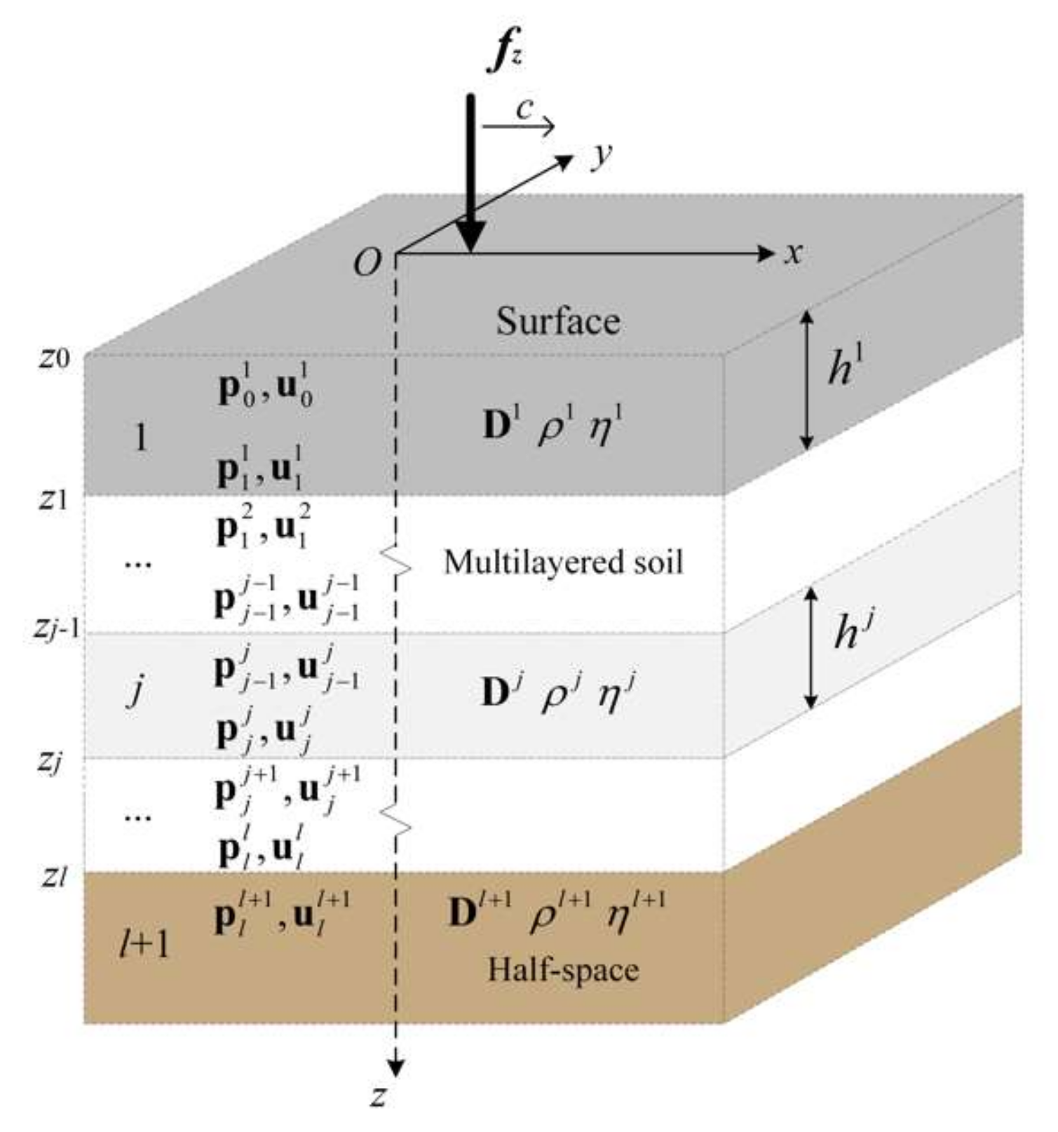
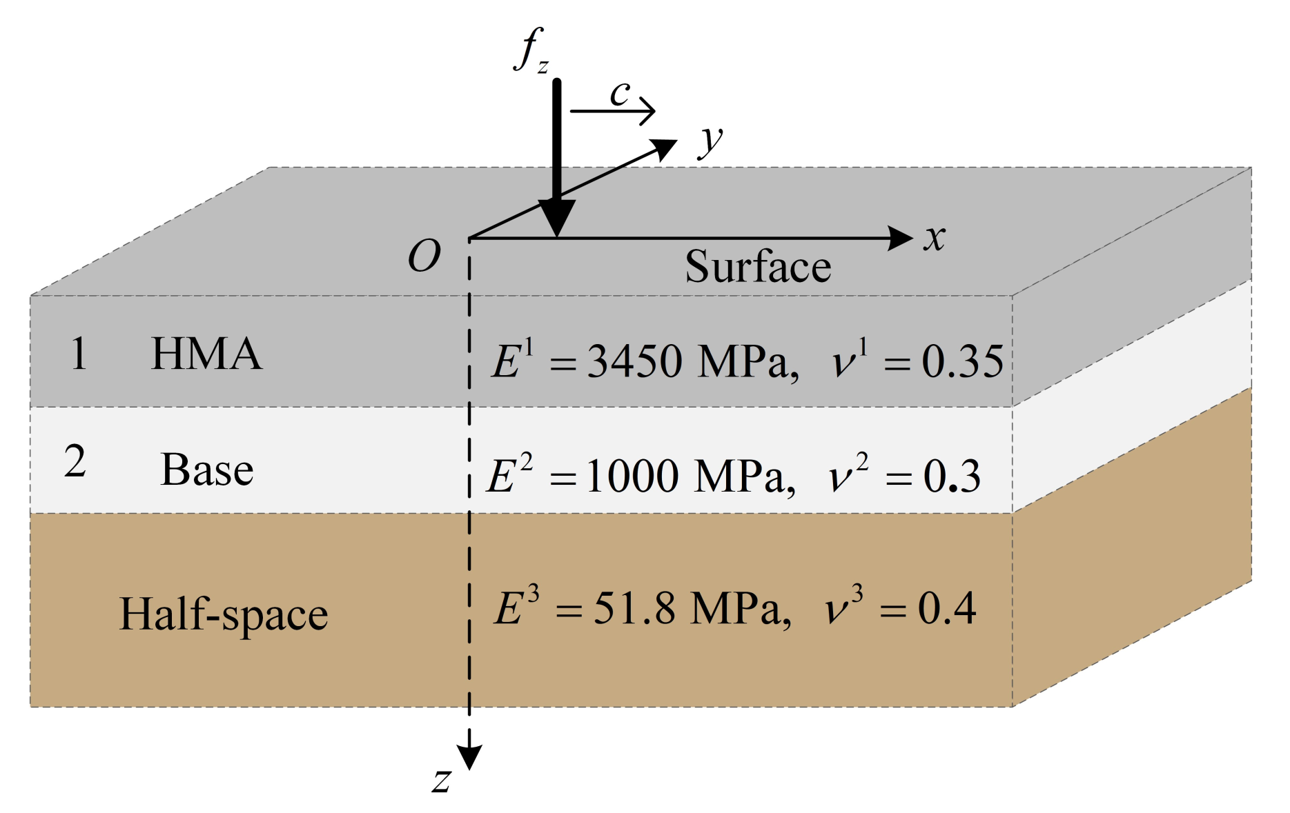
Consider a semi-infinite elastic road structure made up of l+1 horizontal, homogeneous, anisotropic viscoelastic layers which overlies a homogeneous, anisotropic viscoelastic half-space (Figure 1). For the jth layer, the material constants are: the elasticity matrix $D^j$; the mass density, ${\rho }^j$; the hysteretic damping ratio, ${\eta }^j$; and the layer thickness, $h^j$. It is assumed that the z-axis is pointing downward through the medium, with the origin of the axes placed at the surface.

2.1. Governing Equation within the Frequency-Wavenumber Domain for a General Anisotropic Multilayered Medium

According to Hook’s law, the stress–strain relationship in Cartesian coordinates for a general anisotropic material is expressed as follows:

$$\left\{\begin{array}{c}{\underline{{\sigma }}}_x\hfill \\ {\underline{{\sigma }}}_y\hfill \\ {\underline{{\sigma }}}_z\hfill \\ {\underline{\tau }}_{xy}\hfill \\ {\underline{\tau }}_{xz}\hfill \\ {\underline{\tau }}_{yz}\hfill \end{array}\right\}=\left[\begin{array}{cccccc}{d}_{11}\hfill & d_{12}\hfill & d_{13}\hfill & d_{14}\hfill & d_{15}\hfill & d_{16}\hfill \\ d_{21}\hfill & d_{22}\hfill & d_{23}\hfill & d_{24}\hfill & d_{25}\hfill & d_{26}\hfill \\ d_{31}\hfill & d_{32}\hfill & d_{33}\hfill & d_{34}\hfill & d_{35}\hfill & d_{36}\hfill \\ d_{41}\hfill & d_{42}\hfill & d_{43}\hfill & d_{44}\hfill & d_{45}\hfill & d_{46}\hfill \\ d_{51}\hfill & d_{52}\hfill & d_{53}\hfill & d_{54}\hfill & d_{55}\hfill & d_{56}\hfill \\ d_{61}\hfill & d_{62}\hfill & d_{63}\hfill & d_{64}\hfill & d_{65}\hfill & d_{66}\hfill \end{array}\right]\left\{\begin{array}{c}{\underline{\epsilon }}_x\hfill \\ {\underline{\epsilon }}_y\hfill \\ {\underline{\epsilon }}_z\hfill \\ {\underline{\gamma }}_{xy}\hfill \\ {\underline{\gamma }}_{xz}\hfill \\ {\underline{\gamma }}_{yz}\hfill \end{array}\right\}$$

(1)

or briefly

$${\displaystyle \underset{\_}{\mathsf{\sigma }}}=D{\displaystyle \underset{\_}{\mathsf{\epsilon }}}$$

(2)

where $D$ is the elasticity matrix, ${\displaystyle \underset{\_}{\mathsf{\sigma }}}$ is the stress vector, and the strain vector is $\underset{\_}{\mathsf{\epsilon }}=\mathbf{L}{\displaystyle \underset{\_}{\mathbf{u}}}$; ${\displaystyle \underset{\_}{\mathbf{u}}}$ stands for the displacement vector, i.e., $\underset{\_}{\mathbf{u}}=[\begin{array}{ccc}{\underset{\_}{u}}_x& {\underset{\_}{u}}_y& {\underset{\_}{u}}_z\end{array}{]}^{\mathrm{T}}$. The partial differential operator $L$ is expressed as:

$$L={\left[\begin{array}{cccccc}\frac{\partial }{\partial x}& & & \frac{\partial }{\partial y}& \frac{\partial }{\partial z}& \\ & \frac{\partial }{\partial y}& & \frac{\partial }{\partial x}& & \frac{\partial }{\partial z}\\ & & \frac{\partial }{\partial z}& & \frac{\partial }{\partial x}& \frac{\partial }{\partial y}\end{array}\right]}^{\mathrm{T}}$$

(3)

The Lame wave motion equation for a 3D medium, with vanishing body forces, can be formulated as:

$$L^{\mathrm{T}}{\displaystyle \underset{\_}{\mathsf{\sigma }}}=\rho \frac{{\mathrm{d}}^2\underset{\_}{\mathbf{u}}}{\mathrm{d}{t}^2}$$

(4)

where the superscript dots in ${\mathrm{d}}^2\underset{\_}{\mathbf{u}}/\mathrm{d}{t}^2$ denote the second-order partial derivative, with respect to time, t. $\rho$ is the mass density.

For the solution of the problem, a Fourier transform, and its inverse, are performed to convert the variables between the time-space domain and the frequency domain. It can be defined as follows:

$$\overline{\Gamma }\left(x,y,z,\omega \right)=\frac{1}{2\pi }{\displaystyle {\int }_{-\infty }^{\infty }\Gamma \left(x,y,z,t\right)}\hspace{0.33em}{\mathrm{e}}^{-\mathrm{i}\omega t}\mathrm{d}t$$

(5)

$$\Gamma \left(x,y,z,t\right)={\displaystyle {\int }_{-\infty }^{\infty }\overline{\Gamma }\left(x,y,z,\omega \right)}\hspace{0.33em}{\mathrm{e}}^{\mathrm{i}\omega t}\mathrm{d}\omega$$

(6)

where $\omega$ is the angular frequency; $\mathbf{\Gamma }$ is an arbitrary variable in the time-space domain; and $\overline{\Gamma }$ represents the variable $\mathbf{\Gamma }$ in the transformed domain. For a given layer, j, by substituting Equations (1)–(3) into Equation (4) and applying the Fourier transform, one can obtain a transformed wave equation for a homogeneous anisotropic medium in terms of displacements from Equation (4).

$$\begin{array}{l}{D}_{zz}\frac{{\partial }^2\overline{\underset{\_}{\mathbf{u}}}}{\partial z^2}+\left(D_{xz}+D_{zx}\right)\frac{{\partial }^2\overline{\underset{\_}{\mathbf{u}}}}{\partial x\partial z}+\left(D_{yz}+D_{zy}\right)\frac{{\partial }^2\overline{\underset{\_}{\mathbf{u}}}}{\partial y\partial z}\\ +D_{xx}\frac{{\partial }^2\overline{\underset{\_}{\mathbf{u}}}}{\partial x^2}+\left(D_{xy}+D_{yx}\right)\frac{{\partial }^2\overline{\underset{\_}{\mathbf{u}}}}{\partial x\partial y}+D_{yy}\frac{{\partial }^2\overline{\underset{\_}{\mathbf{u}}}}{\partial y^2}+\left(\rho {\omega }^{2}I\right)\overline{\underset{\_}{\mathbf{u}}}=0\end{array}$$

(7)

where $\mathbf{I}$ is a $3\times 3$ unit matrix. The corresponding elasticity matrix $D_{ij}(i,j=x,y,z)$ is derived as

$$\begin{array}{c}{\mathbf{D}}_{zz}=\left[\begin{array}{ccc}{d}_{55}\hfill & d_{56}\hfill & d_{53}\hfill \\ d_{65}\hfill & d_{66}\hfill & d_{63}\hfill \\ d_{35}\hfill & d_{36}\hfill & d_{33}\hfill \end{array}\right];{\mathbf{D}}_{xx}=\left[\begin{array}{ccc}{d}_{11}\hfill & d_{14}\hfill & d_{15}\hfill \\ d_{41}\hfill & d_{44}\hfill & d_{45}\hfill \\ d_{51}\hfill & d_{54}\hfill & d_{55}\hfill \end{array}\right];\hfill \\ {\mathbf{D}}_{yy}=\left[\begin{array}{ccc}{d}_{44}\hfill & d_{42}\hfill & d_{46}\hfill \\ d_{24}\hfill & d_{22}\hfill & d_{26}\hfill \\ d_{64}\hfill & d_{62}\hfill & d_{66}\hfill \end{array}\right];{\mathbf{D}}_{xy}={\mathbf{D}}_{yx}^{\mathrm{T}}=\left[\begin{array}{ccc}{d}_{14}\hfill & d_{12}\hfill & d_{16}\hfill \\ d_{44}\hfill & d_{42}\hfill & d_{46}\hfill \\ d_{54}\hfill & d_{52}\hfill & d_{56}\hfill \end{array}\right];\hfill \\ {\mathbf{D}}_{zx}={\mathbf{D}}_{xz}^{\mathrm{T}}=\left[\begin{array}{ccc}{d}_{15}\hfill & d_{16}\hfill & d_{13}\hfill \\ d_{45}\hfill & d_{46}\hfill & d_{43}\hfill \\ d_{55}\hfill & d_{56}\hfill & d_{53}\hfill \end{array}\right];{\mathbf{D}}_{zy}={\mathbf{D}}_{yz}^{\mathrm{T}}=\left[\begin{array}{ccc}{d}_{45}\hfill & d_{46}\hfill & d_{43}\hfill \\ d_{25}\hfill & d_{26}\hfill & d_{23}\hfill \\ d_{65}\hfill & d_{66}\hfill & d_{63}\hfill \end{array}\right];\hfill \end{array}$$

(8)

The solution of $\overline{\underset{\_}{\mathbf{u}}}$ for Equation (7) is in exponential forms. Based on the assumption that the layered half-space is uniform in the horizontal direction, different waves should have the same phase at the surface $z=0$. Therefore, the solution of $\overline{\underset{\_}{\mathbf{u}}}$ for Equation (7) can be expressed as

$$\overline{\underset{\_}{\mathbf{u}}}={\left[\begin{array}{ccc}{\overline{u}}_x(z)& {\overline{u}}_y(z)& {\overline{u}}_z(z)\end{array}\right]}^{\mathrm{T}}{\mathrm{e}}^{-\mathrm{i}{\kappa }_{x}x}{\mathrm{e}}^{-\mathrm{i}{\kappa }_{x}y}=\overline{u}(z){\mathrm{e}}^{-\mathrm{i}{\kappa }_{x}x}{\mathrm{e}}^{-\mathrm{i}{\kappa }_{x}y}$$

(9)

where ${\kappa }_x$ and ${\kappa }_y$ are the wave numbers along the x-axis and y-axis, respectively. Substituting Equation (9) into Equation (7), one can obtain a transformed wave equation, with the vertical coordinate z serving as a variable, i.e.,

$$C_0^j{\overline{u}}_{,zz}^j+\left(C_1^j-{\left(C_1^j\right)}^{\mathrm{H}}\right){\overline{u}}_{,z}^j-\left(C_2^j-{\rho }^j{\omega }^{2}I\right){\overline{u}}^j=0$$

(10)

Equation (10) is an ordinary differential equation, where ${\overline{u}}_{,z}^j$ is the partial derivative of ${\overline{u}}_{}^j$ with respect to z in the jth layer, and the coefficient matrices for the anisotropic medium in the jth layer take the following form:

$$\begin{array}{l}{C}_0^j=D_{zz}^j\\ C_1^j=-\mathrm{i}{\kappa }_x\left(D_{xz}^j\right)-\mathrm{i}{\kappa }_y\left(D_{yz}^j\right)\\ C_2^j={\kappa }_x^2{D}_{xx}^j+{\kappa }_x{\kappa }_y\left(D_{xy}^j+D_{yx}^j\right)+{\kappa }_y^2{D}_{yy}^j\end{array}$$

(11)

where the effect of damping needs to be considered, the elastic constants in Equation (11) need to be multiplied by $1+2\mathrm{i}{\eta }^j$, (${\eta }^j$ is the hysteretic damping ratio of the jth layer). In order to solve Equation (10), the dual stress vector $p^j=-{\left[\begin{array}{ccc}{\tau }_{xz}^j& {\tau }_{yz}^j& {\sigma }_z^j\end{array}\right]}^{\mathrm{T}}$ for the jth layer is introduced, and by applying the relationships between the stresses and the displacement in the transformed domain, the stress vector can be expressed as follows:

$${\overline{p}}^j=-C_0^j{\overline{u}}_{,z}^j-C_1^j{\overline{u}}^j$$

(12)

By introducing the state vector ${\overline{S}}^j={\left[\begin{array}{cc}{\overline{u}}^j& {\overline{p}}^j\end{array}\right]}^{\mathrm{T}}$ into Equation (10), it can be rewritten as a first-order ordinary differential equation in the frequency-wavenumber domain:

$${\overline{S}}_{,z}^j=H^j{\overline{S}}^j$$

(13)

where $H^j$ is a Hamiltonian matrix, which is expressed as follows:

$$H^j=\left[\begin{array}{cc}-{(C_0^j)}_{}^{-1}{C}_1^j& -{(C_0^j)}_{}^{-1}\\ {\left(C_1^j\right)}^{\mathrm{H}}{(C_0^j)}_{}^{-1}{C}_1^j-C_2^j+{\rho }^j{\omega }^{2}I& {\left(C_1^j\right)}^{\mathrm{H}}{(C_0^j)}_{}^{-1}\end{array}\right]$$

(14)

2.2. Solution of the Transformed Wave Equation

Equation (13) is the governing equation of the wave propagation. The solution can be obtained when the boundary conditions are determined. However, for different materials, such as isotropic, anisotropic, etc., the solutions are different, and the exact solution is very complicated. It should be noted that these solutions exhibit instabilities, such as the case of sharp variations in the stiffness of the layered half-space. In this study, a numerical procedure is used to obtain the solution of Equation (13), which can be used for any medium material and is stable for any layered system.

The general solution of Equation (13) is an exponential function:

$${\overline{S}}^j=\mathbf{exp}(H^{j}z)\left\{c_t\right\}$$

(15)

where $\left\{c_{\mathrm{t}}\right\}$ represents the integration constants. It can be noted that the upper and lower bounds and thickness of the jth layer are $z_{j-1}$, $z_j$, and $h^j=z_j^{}-z_{j-1}^{}$, respectively. According to Equation (15), the state vectors at the upper and lower bounds of the jth layer will satisfy the following:

$${\overline{S}}_j^j=T^j{\overline{S}}_{j-1}^j$$

(16)

where $T^j=\mathbf{exp}(H^j{h}^j)$ is also an exponential function, which is referred to as the state transition matrix.

For calculating the state transition matrix, a precise integration algorithm is applied. The jth layer is divided into $2^N$ min-layers of equal thickness, $h_{\mathrm{mini}}^j=h^j/2^N$, where N is the number of actual integral calculations. Take N = 20 as an example; the integration step is very small, $h_{\mathrm{mini}}^j=h^j/1048576$, which can guarantee calculation accuracy, and the number of integral calculations is a small value: N = 20, which represents the calculation efficiency of the PIA. The exponent $T^j$ can be calculated as follows:

$$T^j=\mathbf{exp}(H^j{h}^j)={[\mathbf{exp}(H^j\frac{h^j}{2^N})]}^{2^N}={[\mathbf{exp}(H^j{h}_{\mathrm{mini}}^j)]}^{2^N}$$

(17)

When performing a Taylor series expansion of the exponent (as $h_{\mathrm{mini}}^j$ is extremely small), this will deviate from the unitary matrix by a small remainder, $T_0$, as shown below:

$$\mathbf{exp}(H^j{h}_{\mathrm{mini}}^j)=I+H^j{h}_{\mathrm{mini}}^j+\frac{{(H^j{h}_{\mathrm{mini}}^j)}^2}{2!}+\frac{{(H^j{h}_{\mathrm{mini}}^j)}^3}{3!}+\frac{{(H^j{h}_{\mathrm{mini}}^j)}^4}{4!}+\cdots =I+T_0^j$$

(18)

$$T_0^j=H^j{h}_{\mathrm{mini}}^j+\frac{{(H^j{h}_{\mathrm{mini}}^j)}^2}{2!}+\frac{{(H^j{h}_{\mathrm{mini}}^j)}^3}{3!}+\frac{{(H^j{h}_{\mathrm{mini}}^j)}^4}{4!}+\cdots$$

(19)

By successively factorizing the exponent, a recursive formula can eventually be obtained for its evaluation:

$$T^j={(I+T_0^j)}^{2^N}={(I+T_1^j)}^{2^{N-1}}=\cdots ={(I+T_{N-1}^j)}^2=I+T_N^j$$

(20)

where

$$\begin{array}{l}{(I+T_0^j)}^2=I+2T_0^j+{(T_0^j)}^2=I+T_1^j,\hspace{0.33em}\hspace{0.33em}\hspace{0.33em}\hspace{0.33em}\hspace{0.33em}{T}_1^j=2T_0^j+{(T_0^j)}^2\\ {(I+T_1^j)}^2=I+2T_1^j+{(T_1^j)}^2=I+T_2^j,\hspace{0.33em}\hspace{0.33em}\hspace{0.33em}\hspace{0.33em}\hspace{0.33em}{T}_2^j=2T_1^j+{(T_1^j)}^2\\ \hspace{0.33em}\hspace{0.33em}\hspace{0.33em}\hspace{0.33em}\hspace{0.33em}\hspace{0.33em}\hspace{0.33em}\hspace{0.33em}\hspace{0.33em}\hspace{0.33em}\hspace{0.33em}\hspace{0.33em}\hspace{0.33em}\hspace{0.33em}\hspace{0.33em}\hspace{0.33em}\hspace{0.33em}\hspace{0.33em}\hspace{0.33em}\hspace{0.33em}\hspace{0.33em}\hspace{0.33em}\hspace{0.33em}\hspace{0.33em}\hspace{0.33em}\hspace{0.33em}\hspace{0.33em}\hspace{0.33em}\hspace{0.33em}\hspace{0.33em}\cdots \end{array}$$

$$T_i^j=2T_{i-1}^j+{(T_{i-1}^j)}^2,\left(i=1,2,\cdots N\right)$$

(21)

By applying Equation (21) N times using $T_0^j$ calculated from Equation (18), $T_N^j$ can be determined with a high degree of accuracy. For example, with N = 20, when the Taylor expansion takes the first four terms, the relative error of the omitted value is approximately $O(h_{\mathrm{mini}}^4)\approx {(h^j)}^4/{10}^{24}$. It should be noted that $O(h_{\mathrm{mini}}^4)$ is smaller than the number of decimal digits for double float-point numbers, which is ${10}^{-16}$. Therefore, it can be considered that the accuracy of $T^j$ will reach the highest accuracy for the computer storage.

2.3. Spectral Element Formulation

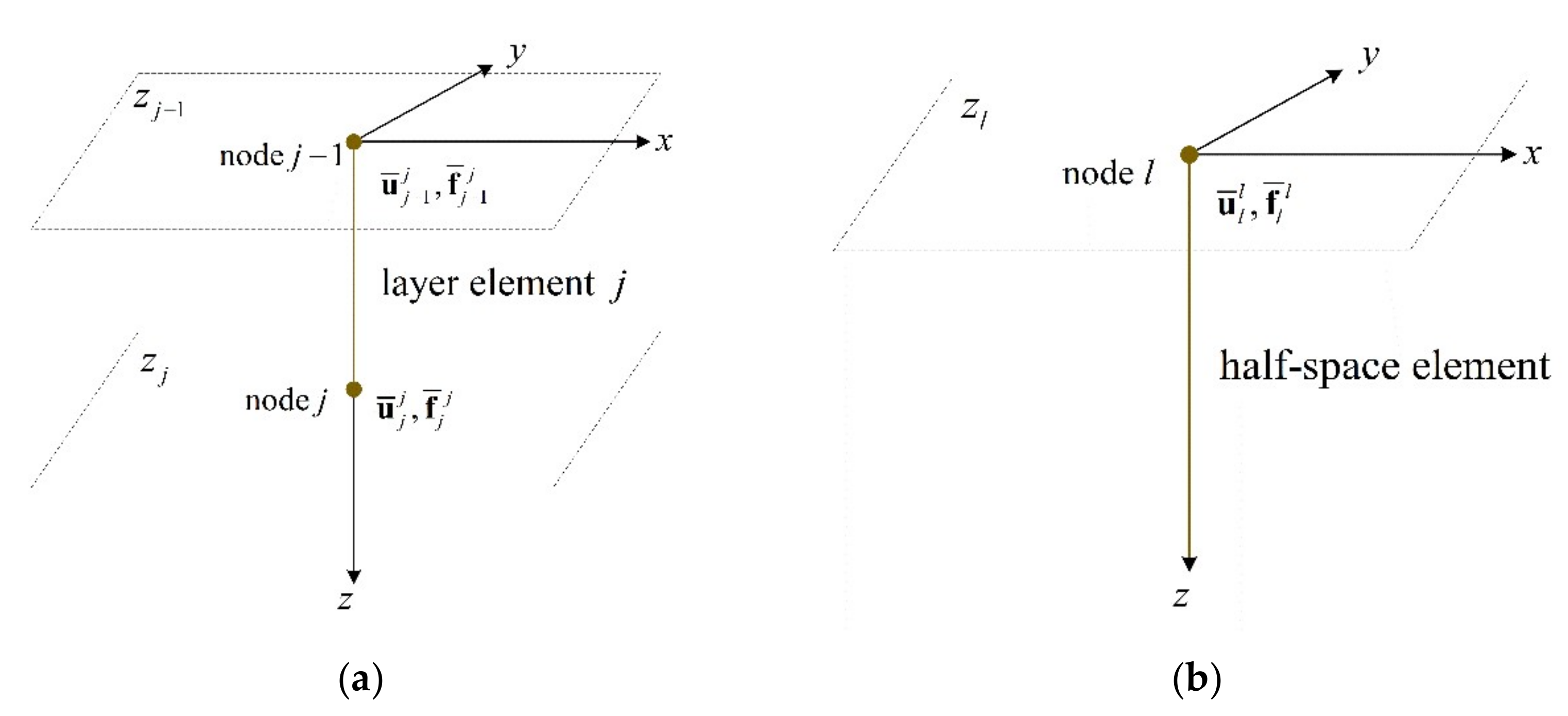
The spectral element method is applied to model the layered system. Based on the state transition matrix, a two-node layer element is developed, and based on the radiation conditions at infinity, a one-node layer element is obtained. In this sub-section, the dynamic stiffness matrix of the two-node layer element and one-node layer element are derived, respectively.

Based on the Cauchy stress principle, for the jth layer element, as shown in Figure 2a, the surface traction of the upper bound is denoted as ${\overline{p}}_{j-1}^j$, and the surface traction of the lower bound is expressed as $-{\overline{p}}_j^j$. The surface traction vector can be expressed as

$$\left\{{\overline{\mathbf{t}}}^j\right\}={\left[\begin{array}{cc}{\left({\overline{\mathbf{f}}}_{j-1}^j\right)}^{\mathrm{T}}& {\left({\overline{\mathbf{f}}}_j^j\right)}^{\mathrm{T}}\end{array}\right]}^{\mathrm{T}}={\left[\begin{array}{cc}{\left({\overline{p}}_{j-1}^j\right)}^{\mathrm{T}}& -{\left({\overline{p}}_j^j\right)}^{\mathrm{T}}\end{array}\right]}^{\mathrm{T}}$$

(22)

in which $\left\{{\overline{\mathbf{t}}}^j\right\}$ is the force vector for the jth layer element, and ${\overline{\mathbf{f}}}_j^j$ is the node force vector. Referring to Figure 1, the continuity conditions relating to the displacements and stresses at the interface between adjacent layer elements can be written as

$${\overline{u}}_j^{}={\overline{u}}_j^j={\overline{u}}_j^{j+1},\hspace{0.33em}\hspace{0.33em}\hspace{0.33em}{\overline{p}}_j^{}={\overline{p}}_j^j={\overline{p}}_j^{j+1},\hspace{0.33em}\hspace{0.33em}\hspace{0.33em}\hspace{1em}(j=1,2,\cdots ,l)$$

(23)

where the superscripts for the displacements and stresses denote the layer number, while the subscripts denote the interface number.

For a natural layer, by using the PIA, the state transition matrix is obtained, which can be indicated in a partitioned matrix as follows:

$$\left\{\begin{array}{c}{\overline{u}}_j^j\\ {\overline{p}}_j^j\end{array}\right\}=\left[\begin{array}{cc}{T}_{\mathrm{uu}}^j& T_{\mathrm{ud}}^j\\ T_{\mathrm{du}}^j& T_{\mathrm{dd}}^j\end{array}\right]\left\{\begin{array}{c}{\overline{u}}_{j-1}^j\\ {\overline{p}}_{j-1}^j\end{array}\right\}$$

(24)

Substituting Equation (22) into Equation (24), the relationship of the nodal traction vector and displacement is obtained as follows:

$$\left\{\begin{array}{c}{\overline{p}}_{j-1}^j\\ -{\overline{p}}_j^j\end{array}\right\}=\left[\begin{array}{cc}{k}_{\mathrm{uu}}^j& k_{\mathrm{ud}}^j\\ k_{\mathrm{du}}^j& k_{\mathrm{dd}}^j\end{array}\right]\left\{\begin{array}{c}{\overline{u}}_{j-1}^j\\ {\overline{u}}_j^j\end{array}\right\}$$

(25)

where $k_{\mathrm{uu}}^j$, $k_{\mathrm{ud}}^j$, $k_{\mathrm{du}}^j$, $k_{\mathrm{dd}}^j$ can be considered as the element dynamic stiffness, and they can be expressed as follows:

$$\begin{array}{l}{k}_{\mathrm{uu}}^j=-{\left(T_{\mathrm{ud}}^j\right)}^{-1}{T}_{\mathrm{uu}}^j,k_{\mathrm{ud}}^j={\left(T_{\mathrm{ud}}^j\right)}^{-1},\\ k_{\mathrm{du}}^j=T_{\mathrm{dd}}^j{\left(T_{\mathrm{ud}}^j\right)}^{-1}{T}_{\mathrm{uu}}^j-T_{\mathrm{du}}^j,k_{\mathrm{dd}}^j=-T_{\mathrm{dd}}^j{\left(T_{\mathrm{ud}}^j\right)}^{-1}\end{array}$$

(26)

The compact form of Equation (25) can be expressed as

$$\left\{{\overline{t}}^j\right\}=\left[{\overline{k}}^j\right]\left\{{\overline{u}}^j\right\}$$

(27)

For a layered system overlying a homogenous elastic half-space, the wave modes reflected from the boundary at the infinite should be removed. Therefore, there are only waves that travel to infinity. For the one-node layer element, as shown in Figure 2b, the state vector in the semi-infinite half-space also satisfies

$${\overline{S}}_{,z}^{l+1}=H^{l+1}{\overline{S}}^{l+1}$$

(28)

That being so, the following eigenvalue problem relating to the infinite half-space needs to be solved.

$$H^{l+1}\Phi =\Phi \Lambda$$

(29)

where $\Lambda$ is the eigenvalue matrix, and $\Phi$ is the corresponding eigenvectors. In the eigenvalue matrix, the positive and negative eigenvalues appear in pairs. The real part of the eigenvalue is positive, which represents the wave traveling from infinity to the surface, and the negative one represents the downward wave.

The eigenvalues of $\Lambda$ are sorted in descending order, according to the real part value.

$$\Lambda =\left[\begin{array}{cc}{\lambda }_i& \\ & -{\lambda }_i\end{array}\right],\Phi =\left[\begin{array}{cc}{\Phi }_{11}& {\Phi }_{12}\\ {\Phi }_{21}& {\Phi }_{22}\end{array}\right]$$

(30)

In order to solve Equation (28), a new vector $Q={\Phi }^{-1}{\overline{S}}^{l+1}$ is introduced. Substituting Equation (29) and $Q$ into Equation (28), the following relationship can be derived:

$$Q_{,z}=\Lambda Q$$

(31)

The solution of Equation (31) can be expressed as

$$Q=\left[\begin{array}{cc}\mathbf{exp}\left(z{\lambda }_i\right)& \\ & \mathbf{exp}\left(-z{\lambda }_i\right)\end{array}\right]\left\{\begin{array}{c}{c}_{g1}\\ c_{g2}\end{array}\right\}$$

(32)

where $c_{g1}$ and $c_{g2}$ are the integration constants. This yields

$${\overline{S}}^{l+1}=\Phi Q=\left[\begin{array}{cc}{\Phi }_{11}& {\Phi }_{12}\\ {\Phi }_{21}& {\Phi }_{22}\end{array}\right]\left\{\begin{array}{c}{c}_{g1}\mathbf{exp}\left(z{\lambda }_i\right)\\ c_{g2}\mathbf{exp}\left(-z{\lambda }_i\right)\end{array}\right\}$$

(33)

The radiation boundary conditions require that there be no upward propagating wave, which means the value of $c_{g1}$ should be equal to zero. In that case, the boundary condition at the bottom interface between the lth layer element and the half-space will be written as

$${\overline{p}}_l^{l+1}=R^{\infty }{\overline{u}}_l^{l+1}$$

(34)

with

$$R^{\infty }={\Phi }_{22}{\Phi }_{12}^{-1}$$

(35)

2.4. Moving Load

The aspects involved in the tire–pavement interaction mechanism include tire contact area and tire contact pressure. The contact area depends upon several factors, including the axle load, tire type, and inflation pressure. These factors, in turn, have an impact on the distribution of the contact pressure. In the real-world, the outline of the contact area is basically a rectangle or an ellipse full of tread patterns [45], and the contact pressure distribution is usually not uniform [46]. However, taking all these factors into account is not straightforward. So, in most studies, the shape of the contact area is simplified to a circle, a rectangle, or an area that combines two semi-circles and one rectangle [47]. Generally, the contact pressure distribution is also assumed to be uniform across the whole contact area.

To the best of our knowledge, the influence of these different simplified models on ground vibration has not yet been studied. In this paper, two types of distribution are considered: one is the uniform rectangular load. The other assumes a two-dimensional Gaussian distribution over an elliptic area, which is similar to the measured tire–pavement contact pressure distribution in [46,48]. We will discuss the ground vibration resulting from each of these two load models (i.e., a rectangular load and a Gaussian bell load) in the time–spatial domain.

2.4.1. Moving Rectangular Load

As shown in Figure 1, a vertical load $f_z(x,y,0,t)$ is applied on the surface of the layered system, which is moving in the positive x direction with a constant velocity of c across the free surface, and it can be expressed as

$$f_z(x,y,0,t)=r(x-ct,y)\underset{\_}{f}(t)$$

(36)

in which $\underset{\_}{f}(t)$ is the function of the time history of a load, and $r(x,y)$ indicates the function of the spatial distribution of the loads. Based on the assumption of a steady state analysis, the loads have a harmonic time dependence, ${\mathrm{e}}^{\mathrm{i}{\omega }_{0}t}$, with ${\omega }_0$ denoting the angular frequency of the loads, which can be expressed as

$$\underset{\_}{f}(t)=F_z{\mathrm{e}}^{\mathrm{i}{\omega }_{0}t}$$

(37)

where $F_z$ is the magnitude of the vertical load. The load in the transform domain can be obtained by the Fourier transform.

$${\overline{f}}_z({\kappa }_x,{\kappa }_y,0,\omega )=\overline{r}({\kappa }_x,{\kappa }_y)\left[\delta \left(\omega -\left({\omega }_0-{\kappa }_{x}c\right)\right)\right]F_z$$

(38)

For a moving rectangular load, this vertical harmonic point load, $F_z$, is distributed uniformly over a rectangular area with a size of $2l_1\times 2l_2$, and it can be expressed as

$$f_z\left(x,y,0,t\right)=\frac{1}{4l_1{l}_2}H\left(l_1^2-{\left(x-ct\right)}^2\right)H\left(l_2^2-y^2\right)F_z{\mathrm{e}}^{\mathrm{i}{\omega }_{0}t}$$

(39)

in which $H(·)$ is the Heaviside step function. The Fourier transform was utilized for the moving rectangular load, with an x-axis and a y-axis, and the load in the transformed domain is obtained as follows:

$${\overline{f}}_{\mathrm{z}}({\kappa }_x,{\kappa }_y,\omega )=\frac{\sin \left({\kappa }_x{l}_1\right)\sin \left({\kappa }_y{l}_2\right)}{{\kappa }_x{\kappa }_y{l}_1{l}_2}\left[\delta \left(\omega -\left({\omega }_0-{\kappa }_{x}c\right)\right)\right]F_z$$

(40)

where $\delta (·)$ denotes the Dirac delta function.

2.4.2. Moving Bell Load

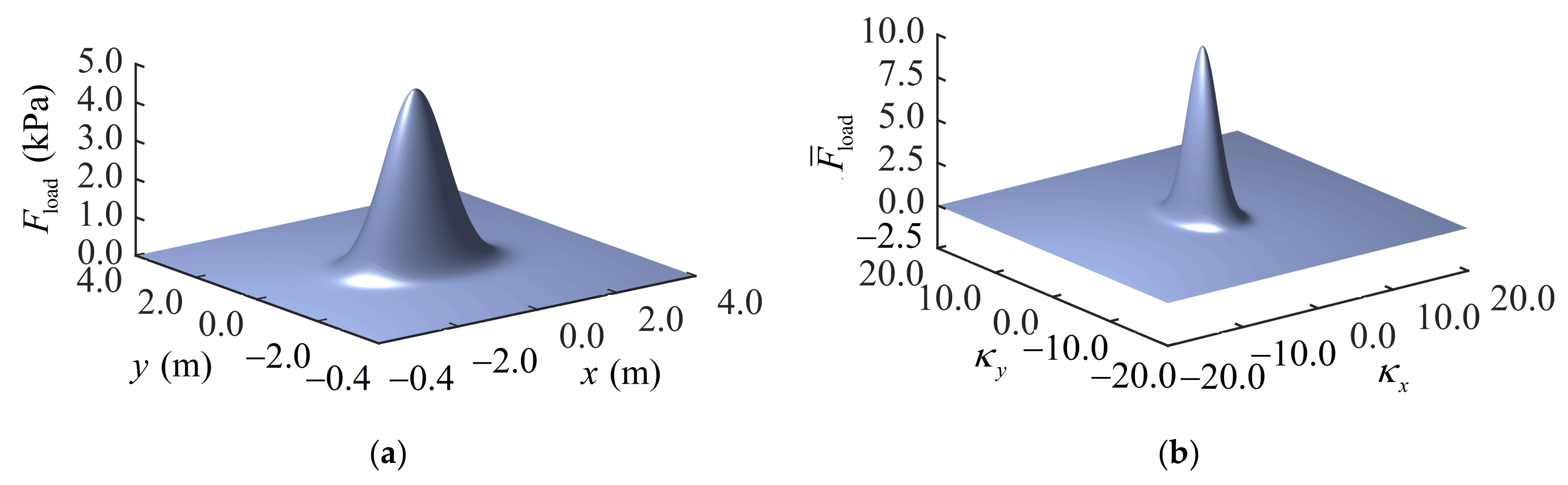
If the vertical harmonic load, $F_z$ is distributed over an elliptical area, with an intensity that obeys a two-dimensional Gaussian distribution. It can be expressed as a moving Gaussian bell load as follows:

$$f_{\mathrm{z}}\left(x,y,0,t\right)=\frac{1}{2\pi {\sigma }_1{\sigma }_2}{\mathrm{e}}^{-\frac{1}{2}\left(\frac{{\left(x-ct-{\mu }_1\right)}^2}{{\sigma }_1^2}+\frac{{(y-{\mu }_2)}^2}{{\sigma }_2^2}\right)}{F}_z{\mathrm{e}}^{\mathrm{i}{\omega }_{0}t}$$

(41)

in which the parameters ${\mu }_1$ and ${\mu }_2$ are expectations in the x and y direction, respectively; the parameters ${\sigma }_1$ and ${\sigma }_2$ are the standard deviation of the bell load, describing how fast the intensity decays in the x and y direction, respectively. In this paper, ${\mu }_1$ and ${\mu }_2$ are set to zero. The Fourier transform was applied to the moving bell load with an x-axis and a y-axis, meaning the load in the transformed domain can be obtained.

$${\overline{f}}_{\mathrm{z}}({\kappa }_x,{\kappa }_y,\omega )=F_z\left[\delta \left(\omega -\left({\omega }_0-{\kappa }_{x}c\right)\right)\right]{\mathrm{e}}^{-\frac{1}{2}\left({\sigma }_1^2{\kappa }_x^2+{\sigma }_2^2{\kappa }_y^2\right)}$$

(42)

2.5. Solution of Layered System

The stiffness matrix of the two-node layer element (Equation (25)) and the one-node layer element (Equation (35)) is assembled via the traditional finite element stiffness matrices for the finite elements in a structure. The global system of equations are expressed as

$${\left\{\begin{array}{c}{\overline{\mathbf{F}}}_0\\ {\overline{\mathbf{F}}}_1\\ {\overline{\mathbf{F}}}_2\\ ⋮\\ {\overline{\mathbf{F}}}_l\end{array}\right\}}^{mn}={\left[\begin{array}{ccccc}{\mathbf{K}}_{\mathrm{uu}}^1& {\mathbf{K}}_{\mathrm{ud}}^1& & & \\ {\mathbf{K}}_{\mathrm{du}}^1& {\mathbf{K}}_{\mathrm{dd}}^1+{\mathbf{K}}_{\mathrm{uu}}^2& {\mathbf{K}}_{\mathrm{ud}}^2& & \\ & {\mathbf{K}}_{\mathrm{du}}^2& {\mathbf{K}}_{\mathrm{dd}}^2+{\mathbf{K}}_{\mathrm{uu}}^3& {\mathbf{K}}_{\mathrm{ud}}^3& \\ & & & \ddots & \\ & & & {\mathbf{K}}_{\mathrm{du}}^l& {\mathbf{K}}_{\mathrm{dd}}^l+{\mathbf{R}}^{\infty }\end{array}\right]}^{mn}{\left\{\begin{array}{c}{\overline{\mathbf{u}}}_0\\ {\overline{\mathbf{u}}}_1\\ {\overline{\mathbf{u}}}_2\\ ⋮\\ {\overline{\mathbf{u}}}_l\end{array}\right\}}^{mn}$$

(43)

with

$${\overline{\mathbf{F}}}_0={\overline{\mathbf{f}}}_0^1,{\overline{\mathbf{F}}}_j={\displaystyle \sum _e{\left\{{\overline{\mathbf{f}}}_j\right\}}^e}={\overline{f}}_j^j+{\overline{\mathbf{f}}}_j^{j+1}\hspace{1em}(j=1,2,\cdots ,l)$$

where m represents the mth wave mode corresponding to the x-axis direction wavenumber ${\kappa }_{xm}$, and n represents the nth wave mode corresponding to the y-axis direction wavenumber ${\kappa }_{yn}$. ${\displaystyle \sum _e}$ represents the summation of layer elements related to interface j. The compact form of the Equation (43) can be expressed as

$${\left\{\overline{\mathbf{F}}(\omega )\right\}}^{mn}={\left[\overline{\mathbf{K}}(\omega )\right]}^{mn}{\left\{\overline{\mathbf{U}}(\omega )\right\}}^{mn}$$

(44)

In practice, the nodal force vector is known, and the displacement is unknown. From Equation (44), the displacement is obtained.

$${\left\{\overline{\mathbf{U}}(\omega )\right\}}^{mn}={\left[\overline{\mathbf{G}}(\omega )\right]}^{mn}{\left\{\overline{\mathbf{F}}(\omega )\right\}}^{mn}$$

(45)

in which ${\left[\overline{\mathbf{G}}(\omega )\right]}^{mn}$ is the inverse of ${\left[\overline{\mathbf{K}}(\omega )\right]}^{mn}$.

For a certain wavenumber, ${\kappa }_{xm}$ and ${\kappa }_{yn}$, the moving load can be achieved by using Equation (40) and Equation (42) for the rectangular loads and the bell loads, respectively. The corresponding nodal force vector can be obtained as follows:

$${\left\{\overline{\mathbf{F}}(\omega )\right\}}^{mn}={\overline{f}}_z({\kappa }_{xm},{\kappa }_{yn},\omega ){\mathbf{E}}_3$$

(46)

in which ${\mathbf{E}}_3$ is the load indication vector, in this case. The third component is one, and the others are zero. According to the theory of SEM, the displacement response is obtained by summing a finite number of wave modes with different discrete frequencies.

$$\mathbf{U}(x,y,t)=F_z{\mathrm{e}}^{\mathrm{i}{\omega }_{0}t}{\displaystyle \sum _n^{}{\displaystyle \sum _m^{}\overline{r}({\kappa }_{xm},{\kappa }_{yn}){\left[\overline{\mathbf{G}}({\omega }_0-{\kappa }_{xm}c)\right]}^{mn}{\mathbf{E}}_3{\mathrm{e}}^{-\mathrm{i}{\kappa }_{xm}(x-ct)}{\mathrm{e}}^{-\mathrm{i}{\kappa }_{yn}y}}}$$

(47)

where the integer m ranges from −M to M, and integer n ranges from −N to N. In order to ensure the accuracy of the solution, M and N should be large enough. The summation of M and N wavenumbers can be carried out by use of the fast Fourier transform (FFT).

It should be noted that only the displacement on the same surface as the nodal elevation can be obtained. If the concerned node lies between two layers, another layer interface is required, passing this node.

3. Numerical Results and Analysis

3.1. Model Verification

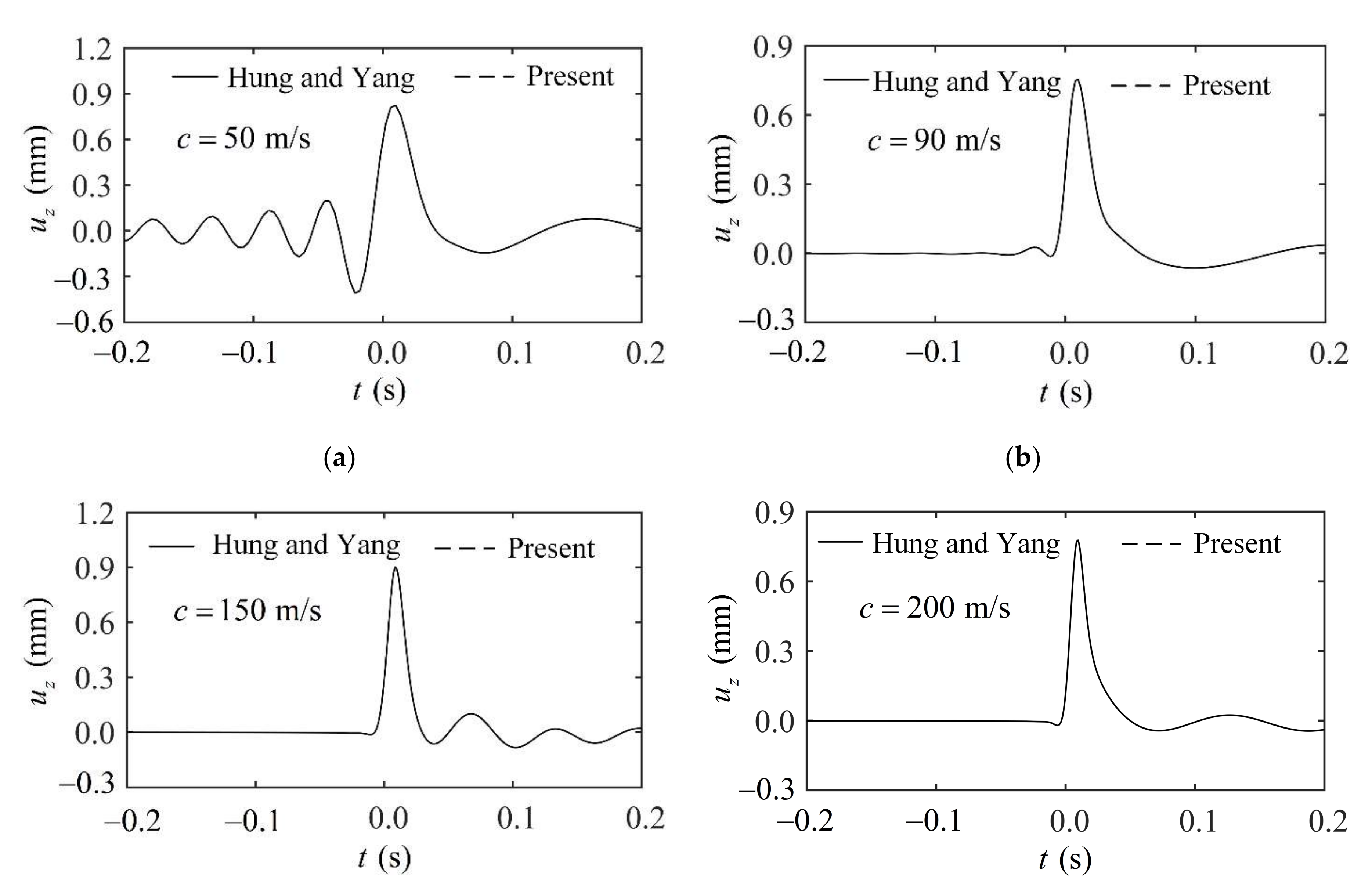
Analytic closed form solutions are often used as a benchmark for testing the accuracy of other methods. In this section, the steady-state responses from the interior of a uniform viscoelastic half-space, investigated by Hung and Yang [49], are compared with the corresponding numerical results obtained by the approach proposed here. In Hung and Yang [49], the Helmholtz potential, a triple Fourier transform, and its inverse, were used to obtain the dynamic responses for different load cases. Taking the case of an elastically distributed wheel load as an example, the viscoelastic half-space considered is assumed to have an S-wave speed of $c_{\mathrm{S}}=100\mathrm{m}/\mathrm{s}$, a P-wave speed of $c_{\mathrm{P}}=173.2\mathrm{m}/\mathrm{s}$, a Rayleigh wave speed of $c_{\mathrm{R}}=92\mathrm{m}/\mathrm{s}$, a Poisson’s ratio of $\nu =0.25$, a mass density of $\rho =2000{\mathrm{kg}/\mathrm{m}}^3$, and a damping ratio of $\eta =0.02$. The numerical results were computed at an observation point of (0, 0, 1), with the wheel load moving at four different speeds: $c=50\mathrm{m}/\mathrm{s}$, $c=90 \mathrm{m}/\mathrm{s}$, $c=150 \mathrm{m}/\mathrm{s}$, and $c=200 \mathrm{m}/\mathrm{s}$, and with a frequency of 10 Hz, as plotted in Figure 3. The elastically moving wheel load in the transformed domain proposed in Hung and Yang [49] would have the form of

$${\overline{f}}_z=\frac{4T}{4+{\kappa }_x^4{\alpha }^4}\delta (\omega -{\omega }_0)$$

(48)

where the axle load was taken to be $T=10\mathrm{t}$ and the characteristic length was $\alpha =0.8 \mathrm{m}$. The angular frequency was ${\omega }_0=20\pi$. By using Equation (47), the displacement of observation point can be obtained. In the analysis, grids measuring 8192 × 8192 were applied, which covers a range of $-32<{\kappa }_x<32$, and $-32<{\kappa }_y<32$.

As indicated in Figure 3, where the instant t = 0 corresponds to the moment where the center of the moving load passes through the origin, the two curves are exactly coincident, and an excellent agreement is reached between the two solutions for the subsonic, transonic, and supersonic cases. This confirms the viability and accuracy of our proposed approach.

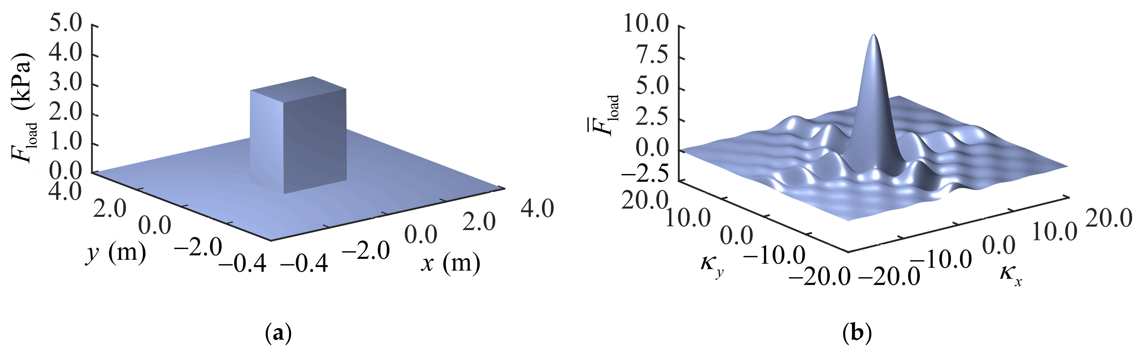
3.2. Effect of Simplified Tire Contact Models

As previously mentioned, a uniformly distributed rectangular load is widely used as the tire contact model in current research. However, in the transformed domain, a rectangular load decays slowly and oscillates infinitely, as shown in Figure 4, which requires the wavenumber range to be set large enough to guarantee its accuracy. It is well known that the Gaussian shape function in the transformed domain is smoother, as shown in Figure 5, which can be transformed more efficiently and conveniently. Therefore, a procedure to convert the uniform rectangular load into an equivalent Gaussian load is derived and validated in this section, which has the benefit of reducing the sampling frequency in the FFT process and, thus, the number of sampling points.

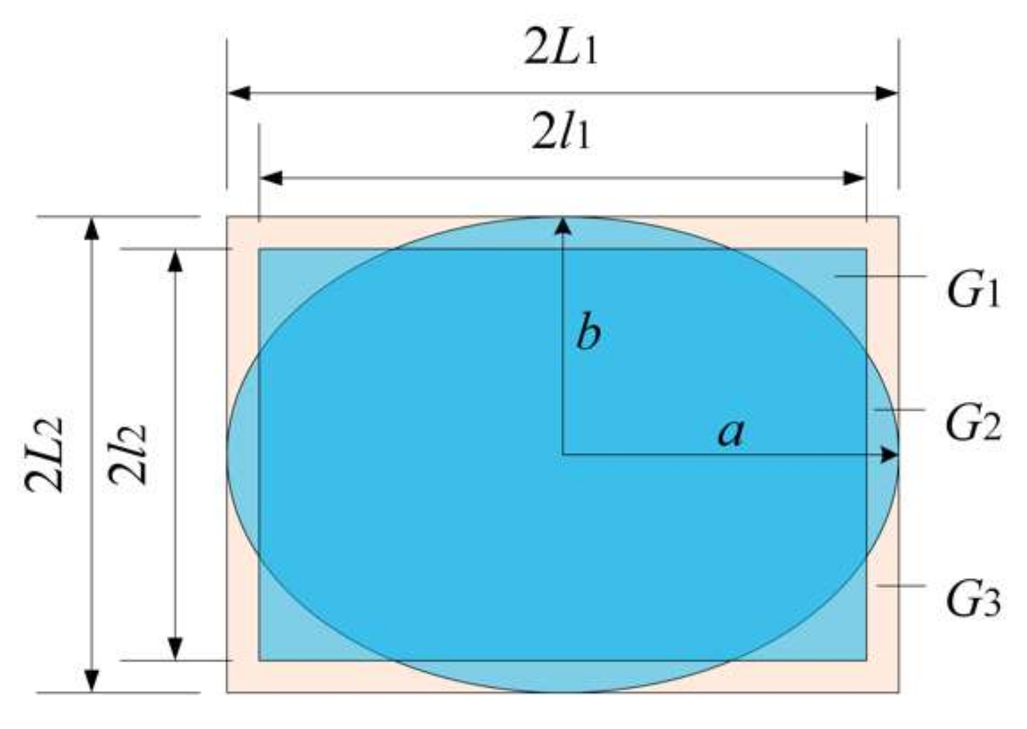
The equivalent conversion rules mentioned above are illustrated in Figure 6. The equivalent criterion is that the resultant force for the different load distributions should be the same. There are three steps that need to be followed:

1.

A uniformly distributed elliptic load in area $G_2$ is set to have an equivalent area to the uniformly distributed rectangular load in area $G_1$. They should have the same dimensional ratio, k, such that $l_2/l_1=k$ and $b/a=k$. This gives the following relationship:

$$\pi ab=4l_1^{}{l}_2^{},a=\frac{2l_1}{\sqrt{\pi }};b=k\frac{2l_1}{\sqrt{\pi }}$$

(49)

2.

The major axis, a, and minor axis, b, of the elliptic load area need to be set to be the long side, L₁, and the short side, L₂, of a new uniform rectangular load area, G₃, respectively;

$$L_1^{}=a=\frac{2l_1}{\sqrt{\pi }};L_2^{}=b=k\frac{2l_1}{\sqrt{\pi }}$$

(50)

3.

This assumes that the expectation and variance of this new rectangular load will be equal to that of the Gaussian bell load in the x-axis and y-axis, respectively.

$${\mu }_1=0,{\mu }_2=0,{\sigma }_1^2=\frac{L_1^2}{3}=\frac{4l_1^2}{3\pi },{\sigma }_2^2=\frac{L_2^2}{3}=k^2\frac{4l_1^2}{3\pi }$$

(51)

By using Equations (41) and (42), and considering Equations (49)–(51), the equivalent Gaussian load of the uniform rectangular load is obtained, which can be used in dynamic analysis.

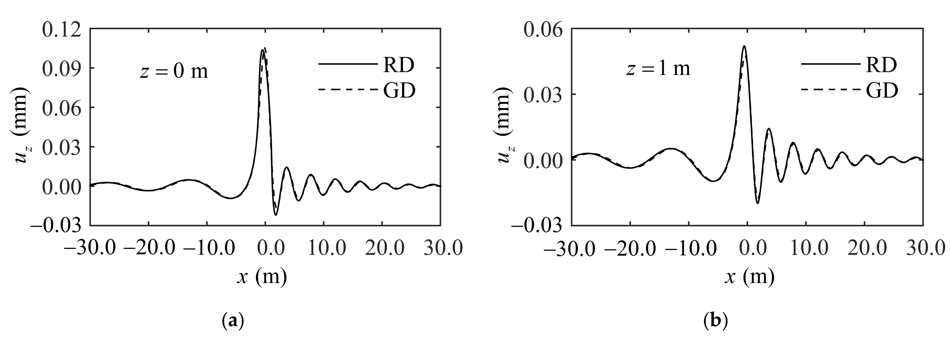
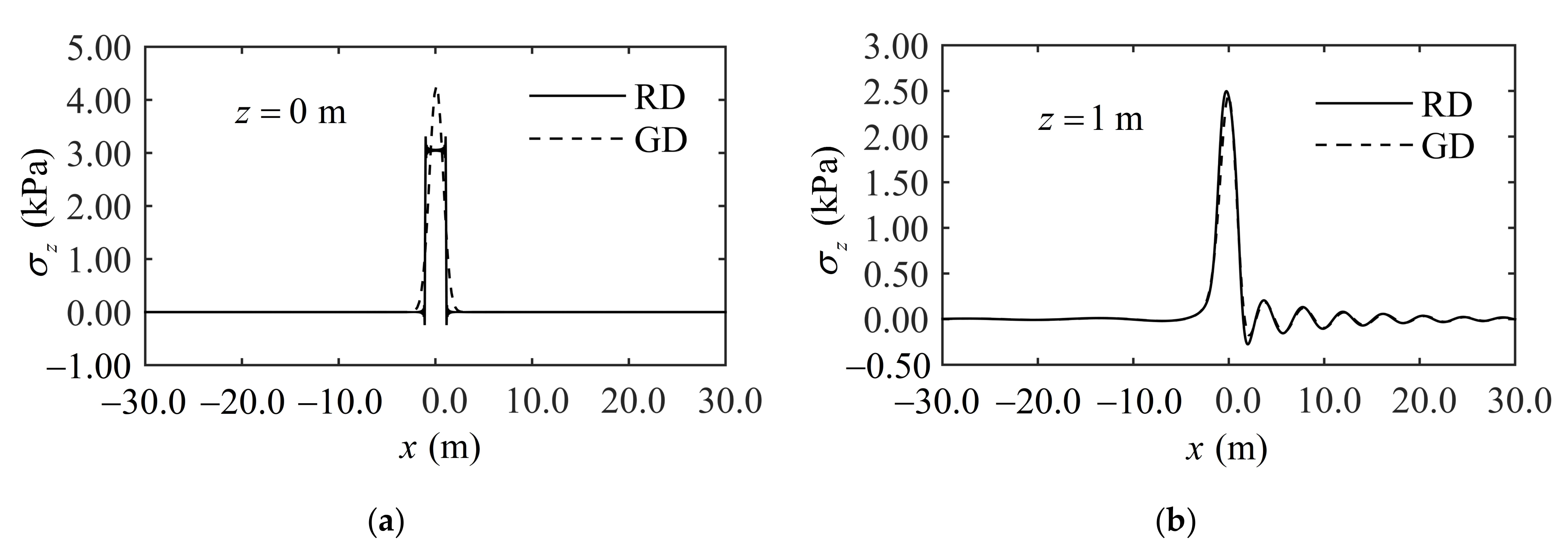
In this section, a study on the effect of load distribution on displacement and stress distribution is considered. Without a loss of generality, the steady-state responses of a uniform viscoelastic half-space caused by a moving load are calculated with different load models. The material properties were the same as in Section 3.1, and the load was taken to be moving at a speed of c = 50 m/s. The other parameters in this study were set such that the resultant force was 10 kN; the dimensional ratio was k = 0.6887 (as recommended in Huang [47]); and the length and width of the uniform rectangular load area were $l_1=1.0854 \mathrm{m}$ and $l_2=0.7475 \mathrm{m}$, respectively. By applying Equations (49)–(51), the standard deviation for the Gaussian bell load was obtained: ${\sigma }_1^{}=0.7071 \mathrm{m}$ and ${\sigma }_2^{}=0.4870 \mathrm{m}$. The comparison of displacement and stress at z = 0 m and z = 1 m for the rectangular load (RD) and Gaussian bell load (GD) are shown in Figure 7 and Figure 8, respectively.

As can be seen from Figure 7, the displacement caused by the rectangular load and the equivalent Gaussian bell load was basically the same. It can also be seen from Figure 8a that the stress at the surface was more affected by the kind of load distribution, though both curves follow the same trend in terms of depth of increase, as can be seen in Figure 8b. So, by following the above equivalent conversion rules, the equivalent load distribution has little effect on the displacement. However, with regard to stress, the distribution near the surface can be significantly influenced by adopting a more realistic tire contact model. This also demonstrates the greater effectiveness of using a Gaussian bell load than a simplified rectangular load. The Gaussian bell load is retained as the load model for the remaining sections.

3.3. Parameter Analysis of Multi-Layered Road

An asphalt road can be idealized as a three-layered system. The top layer is the hot mixed asphalt (HMA) layer; the middle is the base layer, and the bottom is the half-space. Within different design standards, the thickness of the asphalt layer and the base layer are different. Therefore, the effects of the thickness of the HMA layer, base layer, and the moving velocity on the displacement and stress response were investigated. Moreover, the effects of the modulus ratio, as well as the horizontal and vertical modulus of the transverse isotropy, were also studied.

Without losing generality, a three-layer, linear elastic road structure was taken as the object of study. The relevant elastic material constants are shown in Figure 9, and the mass density, ρ = 2000 kg/m³, and the damping ratio, η = 0.02, were adopted for every layer. The reference loading conditions are described as follows: the standard deviation for the Gaussian bell load was ${\sigma }_1={\sigma }_2=0.7071 \mathrm{m}$; the lower speed was c = 50 m/s, and the higher speed was c = 150 m/s; the loading frequency was $f_0=10\mathrm{Hz}$. For the whole parameter sensitivity analysis, grids of 8192 × 8192 for ${\kappa }_x$ and ${\kappa }_y$, which covered a range of [−32, 32], were adopted.

3.3.1. Effects of the Thickness of the HMA Layer

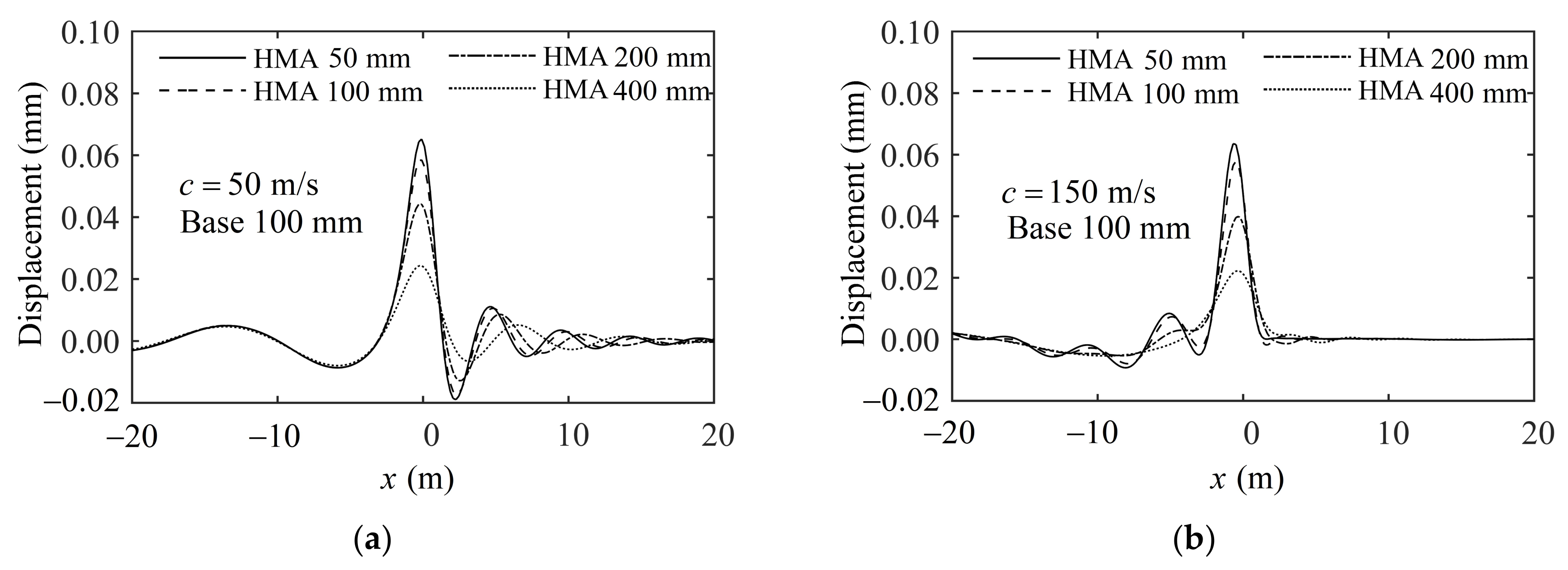
With regard to the effects of the thickness of the HMA layer, only the thickness of the HMA was allowed to vary, while the other parameters were kept constant. For a base thickness of 100 mm and 600 mm, the thicknesses of the HMA were 50 mm, 100 mm, 200 mm, and 400 mm. The dynamic displacements in the z-axis direction of the surface were plotted and are shown in Figure 10.

Figure 10 shows that the fluctuation frequency in front of the load is larger than it is behind it, and a thinner HMA layer may lead to an increase in the fluctuation frequency in front of the load. For both a thinner base and a thicker base, the displacement response of the pavement decreases with the increase of the HMA layer thickness. Note that, in the case of a high-speed moving load with a thinner base, the fluctuation frequency behind the load increases as the HMA layer thickness decreases. It should also be noted that a thinner HMA with a thickness of less than 100 mm can reduce the fluctuation in front of the load, and a HMA layer with a thickness greater than 200 mm can significantly reduce the drastic vibration behind the load. Generally, a 200 mm-thick HMA layer would appear to be a better choice for reducing the displacement response, regardless of the speed of the moving load.

By comparing Figure 10a,b with Figure 10c,d, it can be seen that a thicker base significantly reduces the amplitude of the fluctuations for both low- and high-speed moving loads, and also reduces the fluctuation in front of the load. In practice, the maximum displacement is the most important design indicator. Therefore, the maximum displacement is compared in

Table 1. Reduction in the maximum displacement for different variations in the HMA layer thickness.

HMA	c = 50 m/s				c = 150 m/s
	Base 100 mm		Base 600 mm		Base 100 mm		Base 600 mm
	Maximum (mm)	Reduction	Maximum (mm)	Reduction	Maximum (mm)	Reduction	Maximum (mm)	Reduction
50 mm	0.06522	0.0%	0.02321	0.0%	0.06358	0.0%	0.02146	0.0%
100 mm	0.05853	↓10.3%	0.0205	↓11.7%	0.05787	↓9.0%	0.01931	↓10.0%
200 mm	0.04417	↓32.3%	0.01679	↓27.7%	0.03992	↓37.2%	0.01627	↓24.2%
400 mm	0.0243	↓62.7%	0.01173	↓49.5%	0.02227	↓65.0%	0.01194	↓44.4%

↓ indicates a reduction in the maximum displacement.

. The results in Table 1 show that a reduction in the maximum displacement for a base of 100 mm is greater than it is for a base of 600 mm when the thickness of the HMA layer exceeds 200 mm.

3.3.2. Effects of the Thickness of the Base Layer

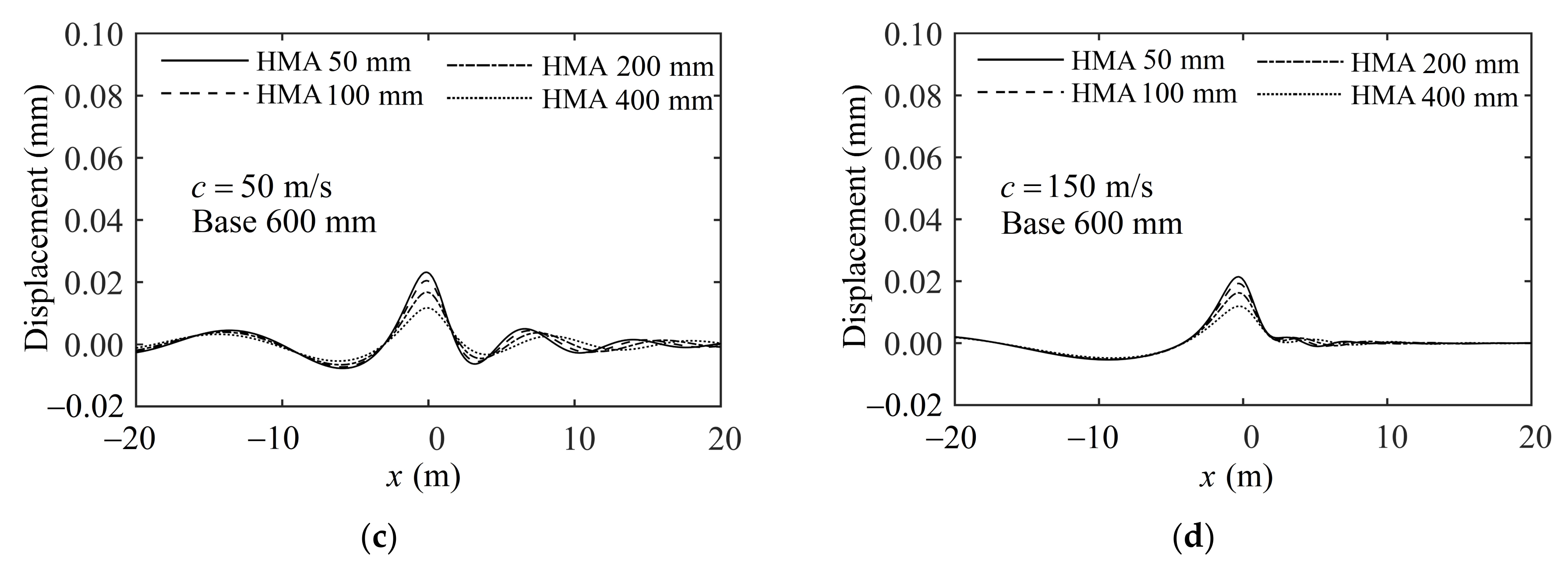
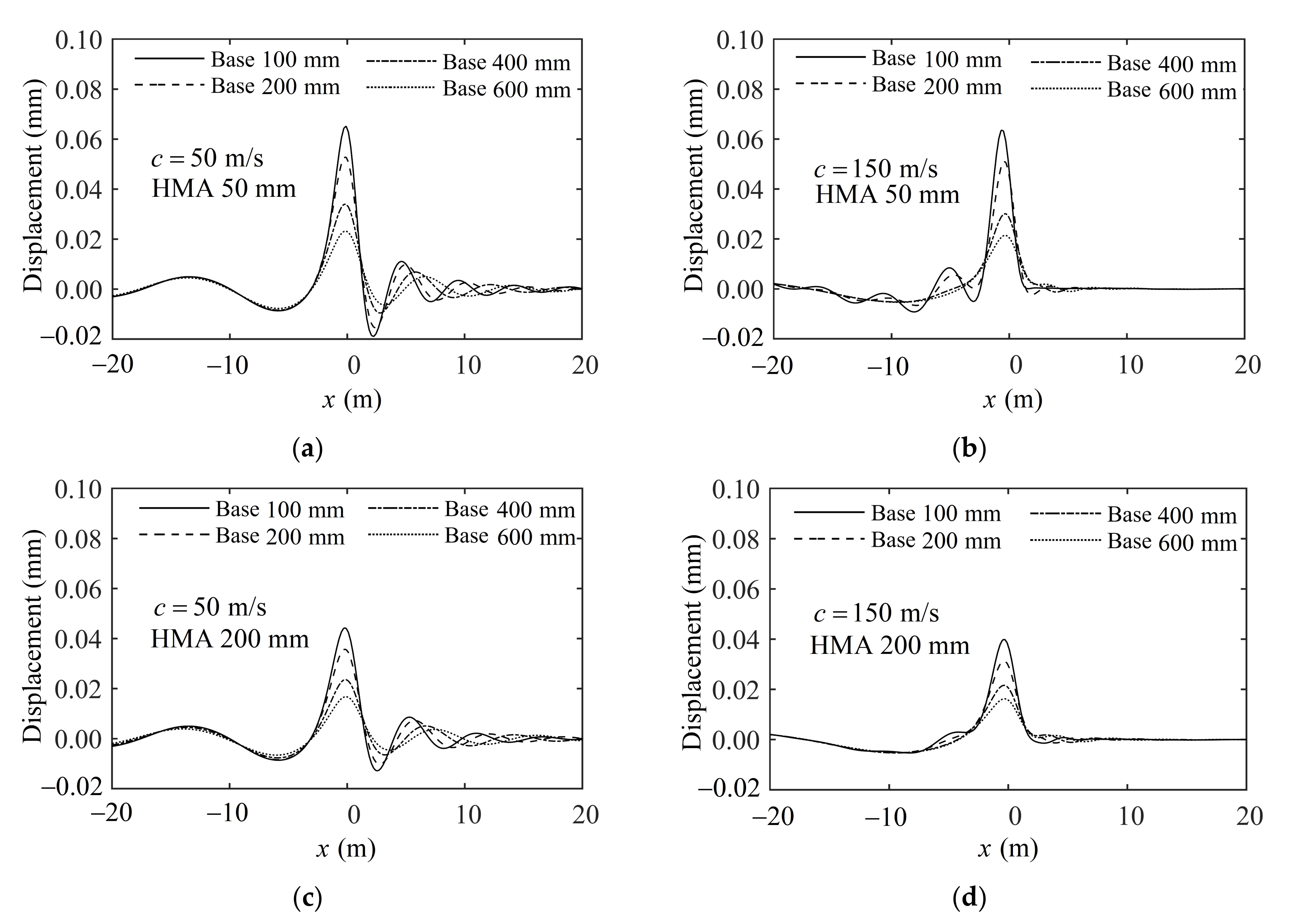
The effects of the thickness of the base layer have been analyzed in sub-Section 3.3.1. However, only two cases were compared, and the overall impression of the effects of the thickness of the base layer is still not clear enough. For this purpose, analyses were conducted for four base layer thicknesses: 100 mm, 200 mm, 400 mm, and 600 mm. The thickness of the HMA layer was 50 mm and 200 mm to provide comprehensive results. Except for the two parameters, all the other parameters for the layered system and the moving loads were kept unchanged. The displacement of the road surface caused by the moving load with a speed of c = 50m/s and c = 150m/s is presented in Figure 11.

Figure 11 shows that as the thickness of the base layer increases, the maximum displacement amplitude decreases significantly. It can be seen that for both a thinner and thicker HMA layer, a base layer with a thickness of 400 mm can reduce the vibration behind the load significantly. In the case of a moving load with a lower speed of c = 50 m/s, except for the amplitudes, the road structures with thinner or thicker HMAs may display the same kind of displacement fluctuation. In the case of a moving load with a higher speed of c = 150 m/s, a thicker base results in a large displacement fluctuation before the arrival of the moving load and then a slight fluctuation after it has passed. The maximum displacement is presented in

Table 2. Reduction in the maximum displacement for different variations in the base layer thickness.

Base	c = 50 m/s				c = 150 m/s
	HMA 50 mm		HMA 200 mm		HMA 50 mm		HMA 200 mm
	Maximum (mm)	Reduction	Maximum (mm)	Reduction	Maximum (mm)	Reduction	Maximum (mm)	Reduction
100 mm	0.06522	0.0%	0.04417	0.0%	0.06358	0.0%	0.03992	0.0%
200 mm	0.05282	↓19.0%	0.03565	↓19.3%	0.05108	↓19.7%	0.03132	↓21.5%
400 mm	0.03397	↓47.9%	0.0236	↓46.6%	0.03014	↓52.6%	0.02163	↓45.8%
600 mm	0.02321	↓64.4%	0.01679	↓62.0%	0.02146	↓66.2%	0.01627	↓59.2%

↓ indicates a reduction in the maximum displacement.

. It can be seen that a reduction in the maximum displacement for HMA layers of 50 mm and 200 mm thicknesses is almost the same. When the thickness of the HMA layer exceeds 400 mm, the reduction in the maximum displacement for the former is slightly larger than it is for the latter. In general, a 400 mm-thick base layer appears to be appropriate for reducing the displacement response, regardless of the speed of the moving load.

3.3.3. Stress, Velocity, and Acceleration Analysis

Generally, there are mutual interactions across a large number of the parameters, and their effect depends not only on any one single parameter itself but also upon the combination of all of the parameters. In this sub-section, the stress, velocity, and acceleration are comprehensively studied and presented to give the overall impression of the effects of the thickness of the HMA layer and base layer.

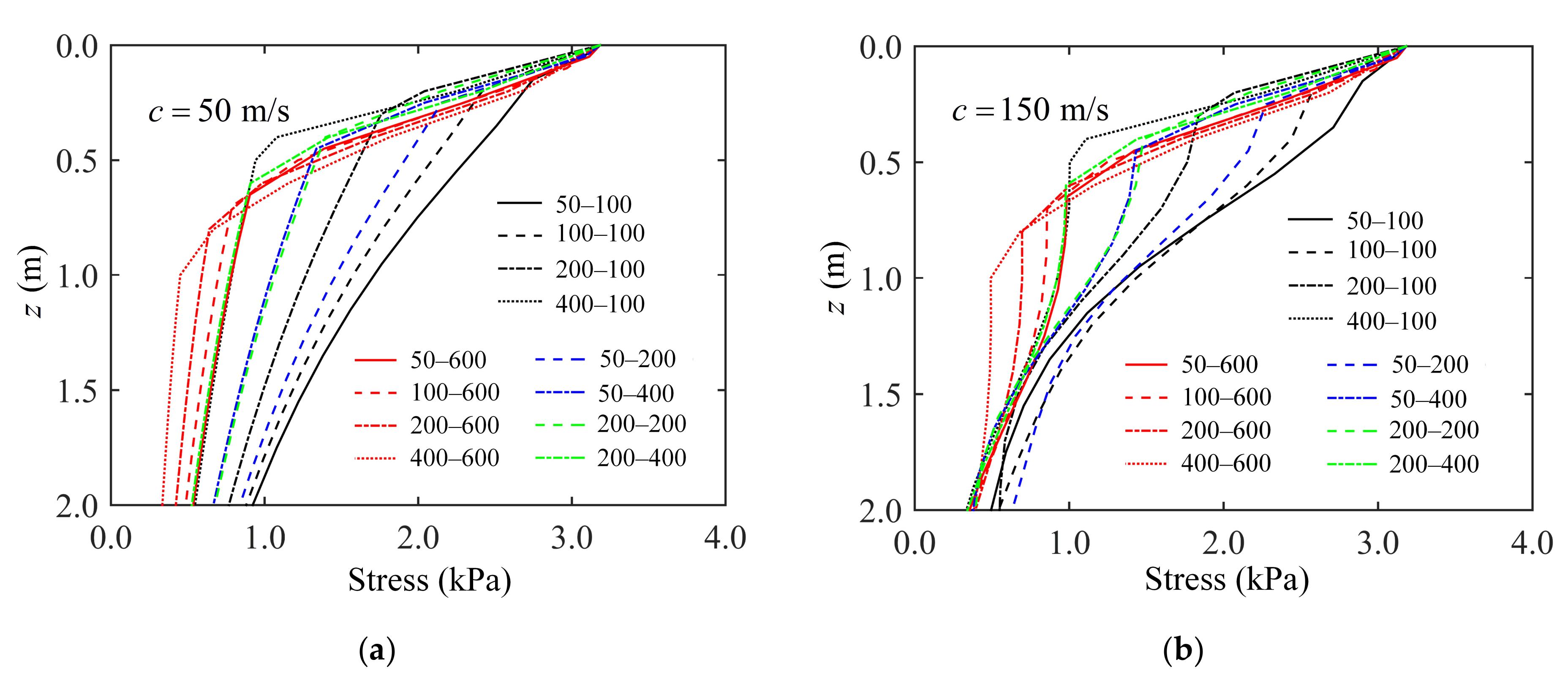
There are various cases for the different combinations of the thickness of the HMA layer and the base layer, which are explained in

Table 3. Cases used for the analysis of the influence of variations in the layer thickness.

Case Type	Thickness of HMA Layer (mm)	Thickness of Base Layer (mm)
50–100	50	100
100–100	100	100
200–100	200	100
400–100	400	100
50–600	50	600
100–600	100	600
200–600	200	600
400–600	400	600
50–200	50	200
50–400	50	400
200–200	200	200
200–400	200	400

. The effect of different proportions of layer thickness on the stress amplitude along the z-axis is shown in Figure 12. It can be seen that a larger total thickness in the various layers results in a smaller minimum value. However, looking at the 50–600 and 200–400 mm cases, things are different. In spite of a smaller total thickness, the latter case of 200–400 mm has a lower minimum value and a faster rate of decrease than the former case. The 400–100 mm case has the fastest rate of decrease but a similar result in the end. Likewise, the 200–200 mm case has a faster rate of decrease than the 50–400 mm case. So, it can be inferred from this that the thickness of the upper HMA layer has a greater influence on the stress along the z-axis than the base does. For cases where the moving load has a higher speed of c = 150 m/s, the results for a depth of more than 1 m show similar changes.

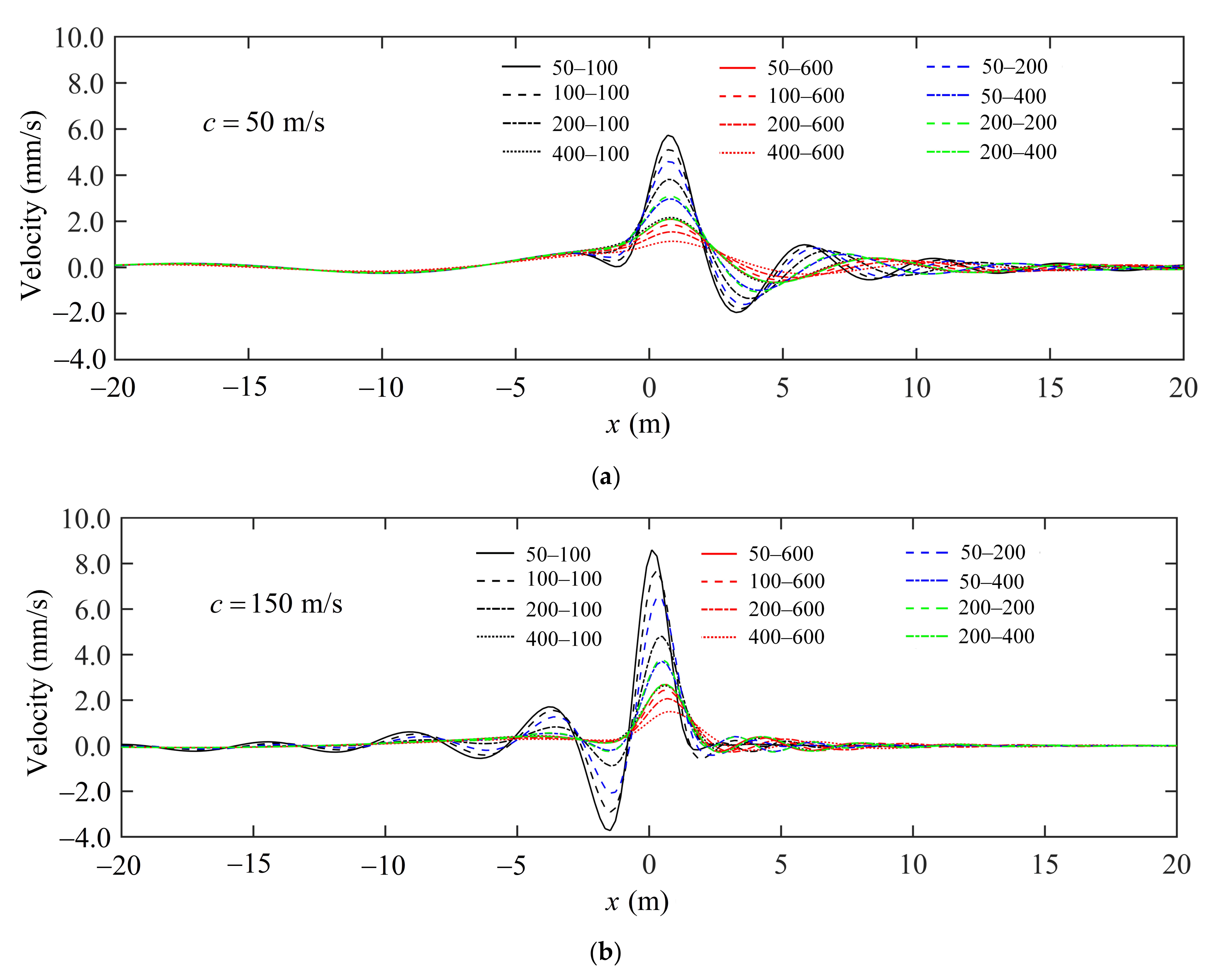
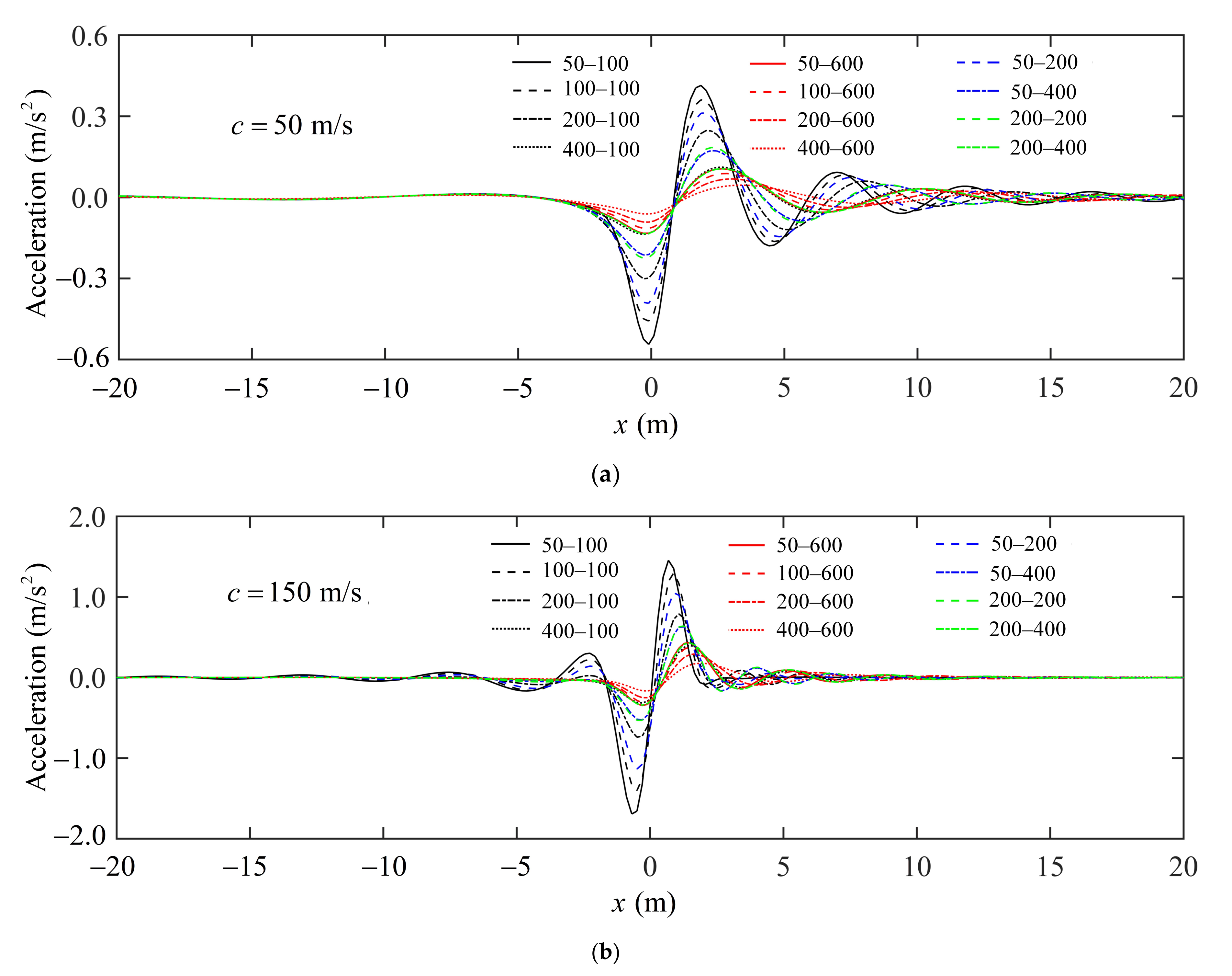
The ground surface vibration velocity and the acceleration along the x-axis are presented in Figure 13 and Figure 14, respectively. This result shows that the changes are the same as they were for the stress under the ground. Note that a thicker overall layer can reduce the degree of tremor. Comprehensive analysis of the results indicates that the 200–400 mm case was the best at reducing dynamic vibration, regardless of the speed of the moving load.

3.3.4. Effects of Modulus Ratio and Transverse Isotropy

In this section, the effects of material anisotropy on the dynamic response of the road are studied. The modulus ratio$n=E_h/E_v$ is usually an important character in representing the character of the transverse isotropy for an elastic medium. $E_h$ and $E_v$ are Young’s modulus in the horizontal direction and in the vertical direction, respectively. To illustrate the influence of $n$ on the HMA and base, the isotropic case from Section 3.3.1 is extended to some transversely isotropic cases, as shown in

Table 4. Cases used for the analysis of the influence of the vertical Young’s modulus of transverse isotropy.

Layers	${\mathit{E}}_{\mathit{h}}(\mathbf{MPa})$	$\mathit{n}={{\mathit{E}}_{\mathit{h}}/\mathit{E}}_{\mathit{v}}$	${\mathit{\nu }}_{\mathit{h}}={\mathit{\nu }}_{\mathit{v}}$	${\mathit{G}}_{\mathit{v}}(\mathbf{MPa})$	Thickness (mm)
HMA	3450	0.5/0.75/1.0	0.35	1277.8	200
Base	1000	0.5 or 1.0	0.30	384.6	400
Half-space	51.8	1.0	0.40	18.5

and

Table 5. Cases used for the analysis of the influence of the horizontal Young’s modulus of transverse isotropy.

Layers	$\mathit{n}={{\mathit{E}}_{\mathit{h}}/\mathit{E}}_{\mathit{v}}$	${\mathit{E}}_{\mathit{v}}(\mathbf{MPa})$	${\mathit{\nu }}_{\mathit{h}}={\mathit{\nu }}_{\mathit{v}}$	${\mathit{G}}_{\mathit{v}}(\mathbf{MPa})$	Thickness (mm)
HMA	0.5/0.75/1.0	3450	0.35	1277.8	200
Base	0.5 or 1.0	1000	0.30	384.6	400
Half-space	1.0	51.8	0.40	18.5

. Three modulus ratios, $n$, for the HMA are considered: n^HMA = 0.5, 0.75, and 1.0, respectively, for which the effect of the base modulus ratio is also taken into consideration, with n^Base being set to 0.5 and 1.0, respectively (see Wang et al. [50] for the rationality of the assumed values). For the investigation into the influence of the vertical Young’s modulus, we kept the horizontal Young’s modulus of the layers unchanged, and took different values of $n^{\mathrm{HMA}}$ and $n^{\mathrm{Base}}$, as shown in Table 4. Similarly, as shown in Table 5, the vertical Young’s modulus of the layers was kept invariant, and the influence of the horizontal Young’s modulus was investigated by varying $n^{\mathrm{HMA}}$ and $n^{\mathrm{Base}}$. The other parameters are the same as those in Section 3.3.1, and two load speeds, measuring c = 50 m/s and c = 150 m/s, were considered. The vertical displacement along the x-axis at the road’s surface are presented in Figure 15 and Figure 16, and the vertical stress at the lower bound of the base layer are presented in Figure 17 and Figure 18.

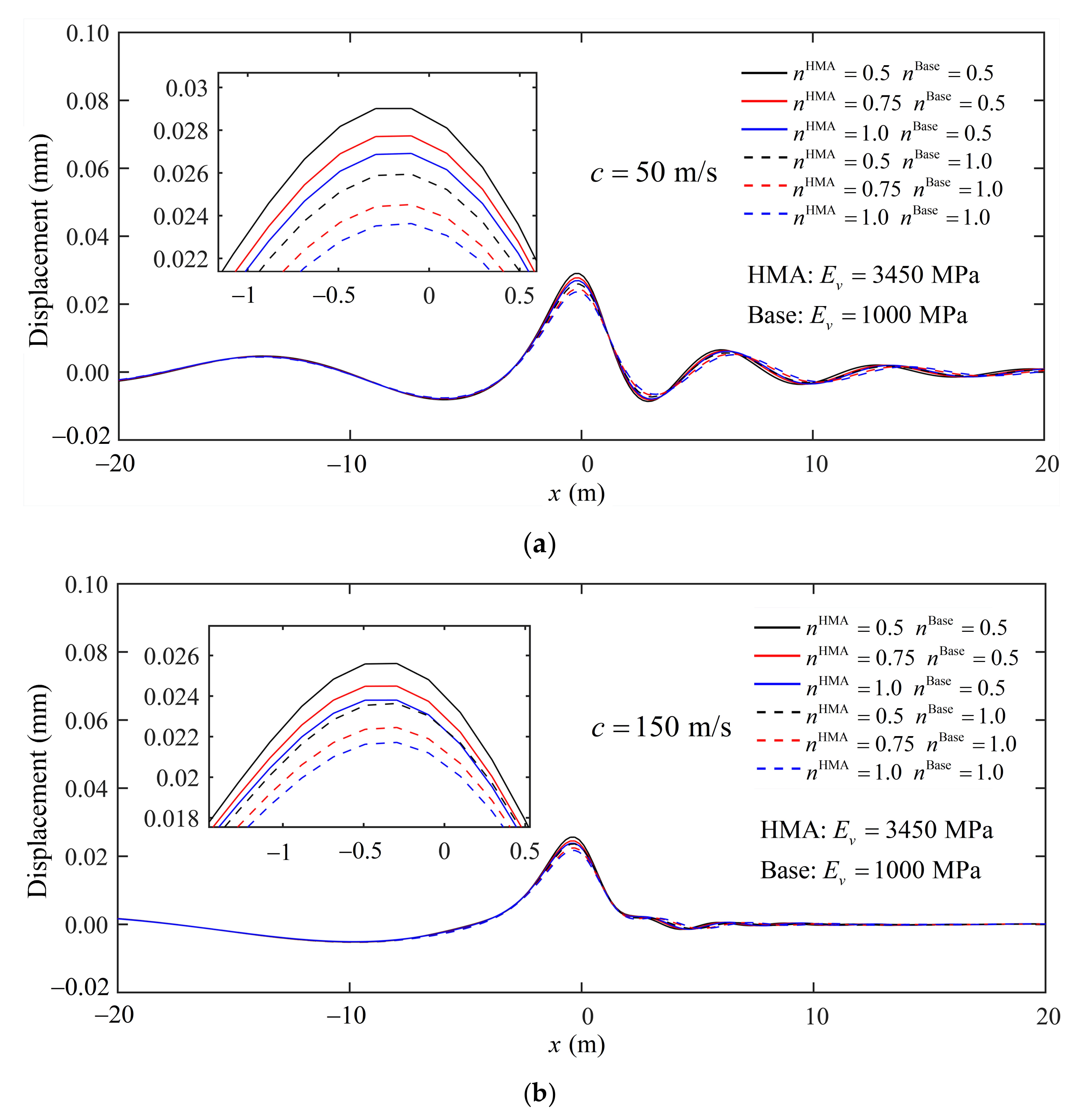
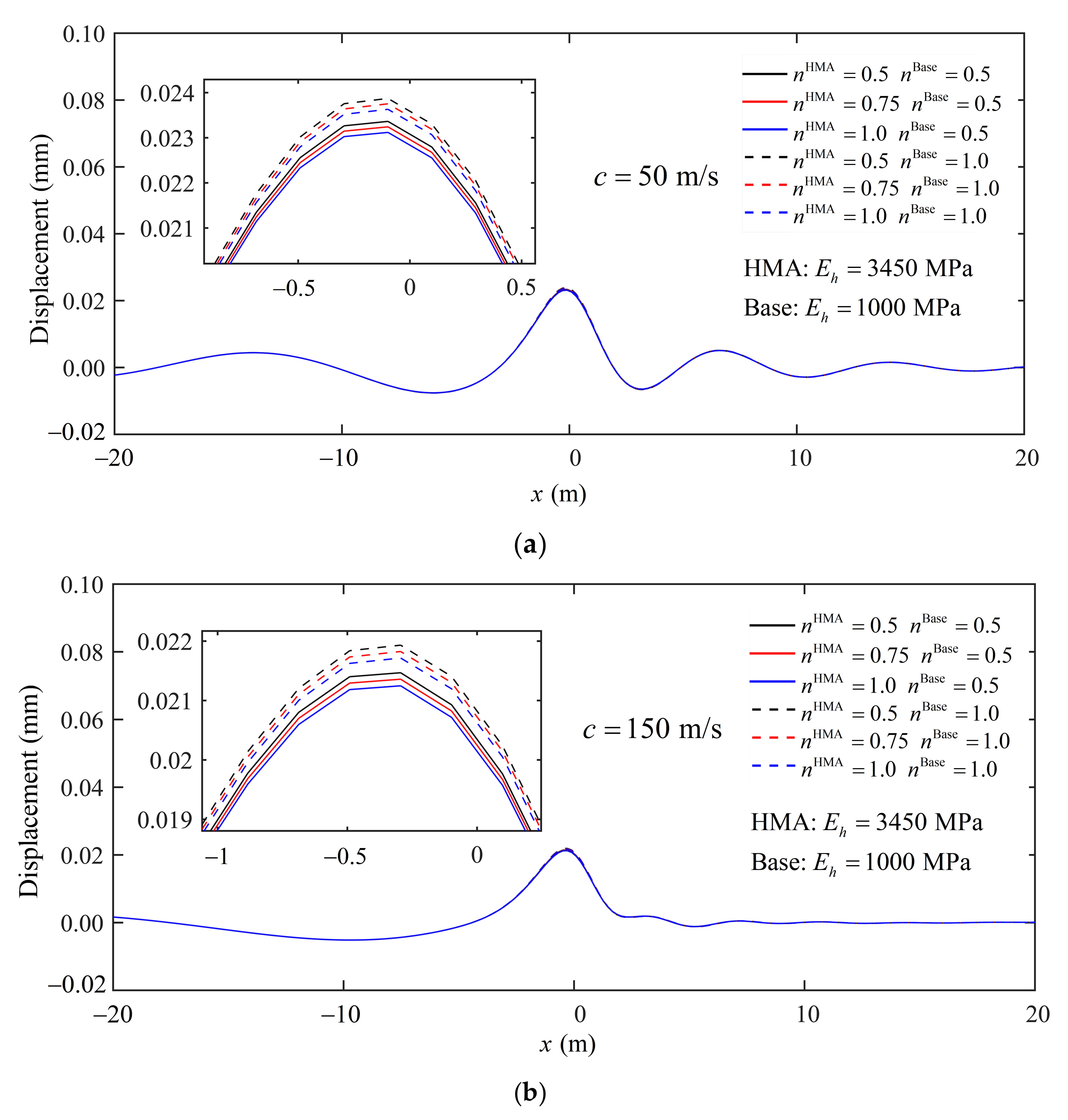
It can be observed from Figure 15 that the modulus ratio, n, of the HMA and the base has a noteworthy impact on the vertical displacement amplitude, in the case of a fixed vertical modulus, $E_v$, for both c = 50 m/s and c = 150 m/s. The vertical displacement decreases as the modulus ratio n^HMA increases due to the increase in the horizontal Young’s modulus, $E_h$, and a larger n^Base for the base layer can significantly decrease the displacement amplitude. In comparison, in the case of a fixed vertical modulus, $E_h$ (Figure 16), the modulus ratio, n, of the HMA and the base has a slight impact on the vertical displacement for both c = 50 m/s and c = 150 m/s. It can still be seen that from the partially enlarged view of the maximum displacement in Figure 16, the vertical displacement decreases as the modulus ratio, n^HMA, increases due to the decrease in the vertical Young’s modulus $E_v$. For both cases (Figure 15 and Figure 16), it can be found that with the increase in the modulus ratio, n^Base, of the base layer, the maximum value of vertical displacement increases.

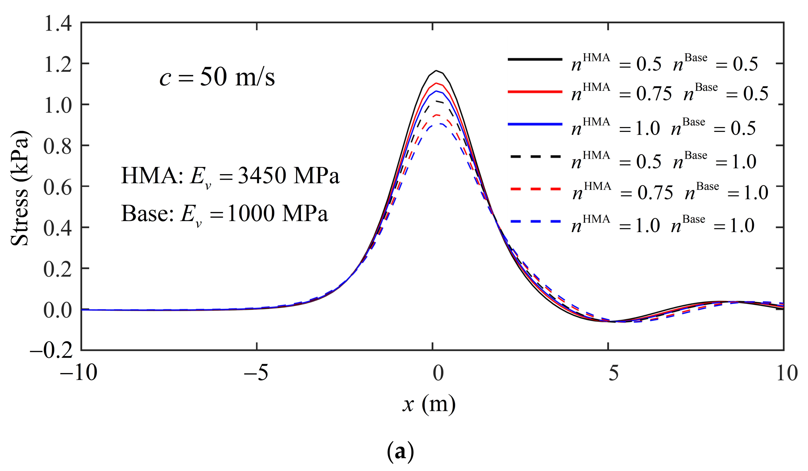
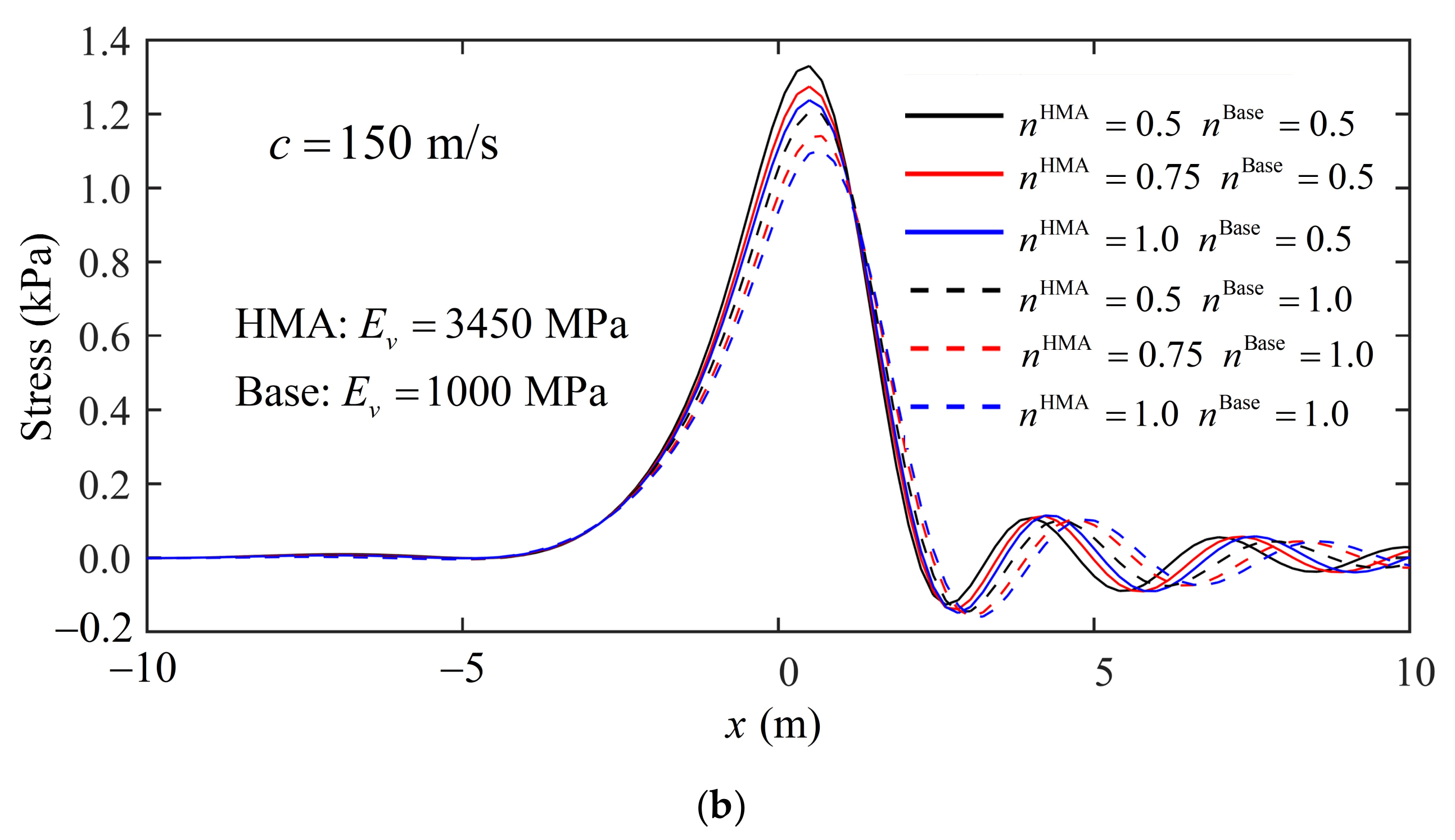
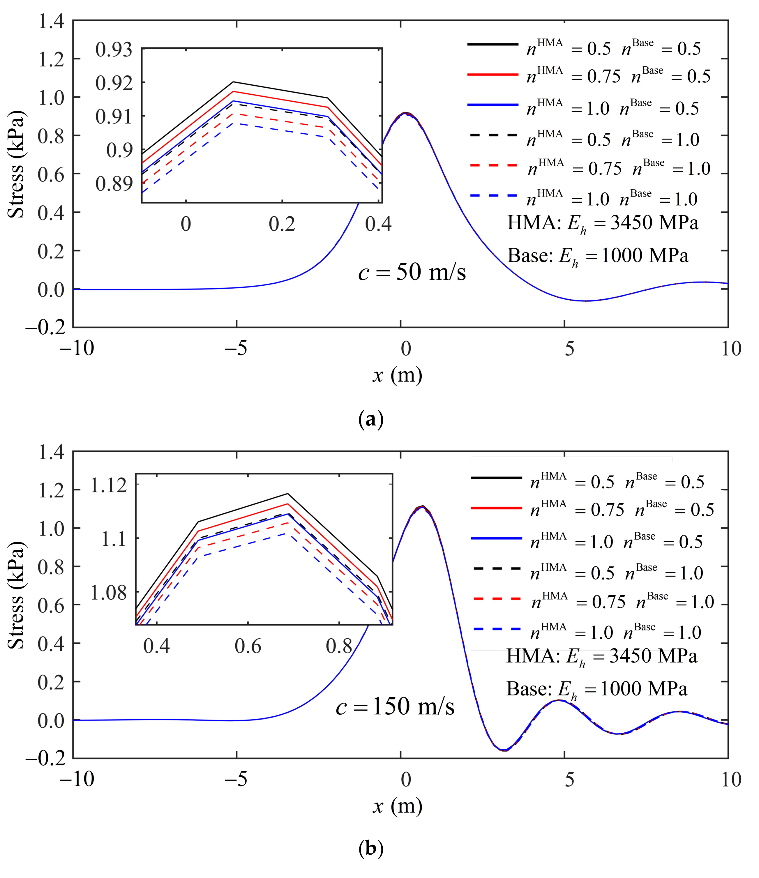
With regards to stress, the distribution of vertical stress along the x direction at the lower bound of the base layer is picked up, as indicated in Figure 17 and Figure 18. It is obvious that, in the case of the fixed vertical modulus (Figure 17), the vertical stress amplitude decreases with the increase in either n^HMA or n^Base for both lower and higher speeds of the moving load. The frequency of the vertical stress fluctuations decreases with an increase in the modulus ratio, n. For a fixed horizontal modulus (Figure 18), the effect of the layer modulus ratio, n^HMA, on the stress amplitude is relatively slight, regardless of whether the base has a small or a large n^Base. However, it can still be observed that as the n^HMA increases due to the decrease in the vertical Young’s modulus $E_v^{}$, the maximum amplitude of stress decreases. A larger vertical modulus, $E_v^{}$, of the base can increase the vertical stress amplitude at the base lower bound. In general, the horizontal Young’s modulus, $E_h$, of the HAM and the base has a significant effect on the dynamic response of the road than does the vertical Young’s modulus, $E_v$, and a larger $E_h$ can reduce the amplitude of both displacement and stress. A smaller vertical Young’s modulus, $E_v$, of the HMA layer can help decrease the dynamic responses, while a base with a smaller $E_v$ can increase the displacement amplitude.

4. Conclusions

This paper presents a modified spectral element model suiigure for solving the dynamic response of a 3D, multilayered, elastic half-space regarding a moving load based on a state transition matrix and a precise integration algorithm. Numerical examples have confirmed the reliability and precision of the proposed procedure through a series of comparisons between existing solutions for both subsonic and supersonic cases. The main advantage of the proposed method is its robustness and versatility. It can be used to analyze wave propagation in an isotropic- or anisotropic-layered half-space without additional work. An equivalent conversion rule was used to simplify the uniform rectangular load typically used in tire contact models to a Gaussian bell load, resulting in a reduction in the number of sampling points in the FFT procedure. The numerical example shows the accuracy of the equivalent conversion rule.

For a fixed modulus in both base and HMA layers, it was found that thicker HMA and base layers can reduce the amplitude of the fluctuations in the response. As the HMA thickness increases, the decrease ratio for the maximum displacement of the base layer, with a thickness of 600 mm, is no more significant than it is for a base layer with a thickness of 100 mm. However, a thicker base layer can reduce the response noticeably if the thickness of the HMA layer is less than 100 mm. The vertical stress along the z axis decreases more rapidly if the thickness of the HMA layer increases. So, overall, the most effective way to decrease the response is to increase the thickness of the HMA layer.

With regards to the transverse isotropy, it was found that a larger horizontal Young’s modulus, $E_h$, for either the HAM or base layer can help reduce the amplitude of the displacement and stress. As the vertical Young’s modulus, $E_v$, of the HMA layer increases, the maximum displacement at the road surface and the maximum stress at the lower bound of the base increase. A base layer with a smaller $E_v$ can decrease the maximum stress, and can increase the maximum displacement. However, the horizontal Young’s modulus, $E_h$, of the HAM or base layer has a significant effect on the dynamic response when compared to the vertical Young’s modulus,$E_v$.

The results in this paper relate to a three-layer road structure that was subjected to a single moving harmonic load. For other elastic multilayered systems with multiple moving loads, obtaining the response will require the adoption of a similar approach and the principle of superposition. The present solutions may be valuable for developing analytical formulations for the analysis of problems involving an anisotropic multilayered medium.

References

- Beskou, N.D.; Theodorakopoulos, D.D. Dynamic Effects of Moving Loads on Road Pavements: A Review. Soil Dyn. Earthq. Eng. 2011, 31, 547–567. [Google Scholar] [CrossRef]
- Thomson, W.T. Transmission of Elastic Waves through a Stratified Solid Medium. J. Appl. Phys. 1950, 21, 89–93. [Google Scholar] [CrossRef]
- Haskell, N.A. The Dispersion of Surface Waves on Multilayered Media. Bull. Seismol. Soc. Am. 1953, 43, 17–34. [Google Scholar] [CrossRef]
- Kausel, E.; Roësset, J.M. Stiffness Matrices for Layered Soils. Bull. Seismol. Soc. Am. 1981, 71, 1743–1761. [Google Scholar] [CrossRef]
- Kausel, E.; Peek, R. Dynamic Loads in the Interior of a Layered Stratum: An Explicit Solution. Bull. Seismol. Soc. Am. 1982, 72, 1459–1481. [Google Scholar] [CrossRef]
- Gunaratne, M.; Sanders III, O. Response of a Layered Elastic Medium To a Moving Strip Load. Int. J. Numer. Anal. Methods Geomech. 1996, 20, 191–208. [Google Scholar] [CrossRef]
- Lefeuve-Mesgouez, G.; Peplow, A.T.; Le Houédec, D. Surface Vibration Due to a Sequence of High Speed Moving Harmonic Rectangular Loads. Soil Dyn. Earthq. Eng. 2002, 22, 459–473. [Google Scholar] [CrossRef]
- Lefeuve-Mesgouez, G.; Messgouez, A. Three-Dimensional Dynamic Response of a Porous Multilayered Ground under Moving Loads of Various Distributions. Adv. Eng. Softw. 2012, 46, 75–84. [Google Scholar] [CrossRef]
- Grundmann, H.; Lieb, M.; Trommer, E. The Response of a Layered Half-Space to Traffic Loads Moving along Its Surface. Arch. Appl. Mech. 1999, 69, 55–67. [Google Scholar] [CrossRef]
- Kausel, E. Generalized Stiffness Matrix Method for Layered Soils. Soil Dyn. Earthq. Eng. 2018, 115, 663–672. [Google Scholar] [CrossRef]
- De Barros, F.C.P.; Luco, J.E. Response of a Layered Viscoelastic Half-Space to a Moving Point Load. Wave Motion 1994, 19, 189–210. [Google Scholar] [CrossRef]
- De Barros, F.C.P.; Luco, J.E. Stresses and Displacements in a Layered Half-Space for a Moving Line Load. Appl. Math. Comput. 1995, 67, 103–134. [Google Scholar] [CrossRef]
- Luco, J.E.; Apsel, R.J. On the Green’s Functions for a Layered Half-Space. Part I. Bull. Seismol. Soc. Am. 1983, 73, 909–929. [Google Scholar] [CrossRef]
- Apsel, J.R.; Luco, J.E. On the Green’s Functions for a Layered Half-Space. Part 2. Bull. Seismol. Soc. Am. 1983, 73, 931–951. [Google Scholar] [CrossRef]
- Sheng, X.; Jones, C.J.C.; Petyt, M. Ground Vibration Generated by a Harmonic Load Acting on a Railway Track. J. Sound Vib. 1999, 225, 3–28. [Google Scholar] [CrossRef]
- Sheng, X.; Jones, C.J.C.; Petyt, M. Ground Vibration Generated by a Load Moving along a Railway Track. J. Sound Vib. 1999, 228, 129–156. [Google Scholar] [CrossRef]
- Jones, C.J.C.; Sheng, X.; Petyt, M. Simulations of Ground Vibration from a Moving Harmonic Load on a Railway Track. J. Sound Vib. 2000, 231, 739–751. [Google Scholar] [CrossRef]
- Chen, S.; Wang, D.; Feng, D.; Guo, D. Fast and Accurate Method for Calculating the Surface Mechanical Responses of Asphalt Pavements. J. Eng. Mech. 2020, 146, 04020090. [Google Scholar] [CrossRef]
- Beskou, N.D.; Muho, E.V.; Qian, J. Dynamic Analysis of an Elastic Plate on a Cross-Anisotropic Elastic Half-Space under a Rectangular Moving Load. Acta Mech. 2020, 231, 4735–4759. [Google Scholar] [CrossRef]
- Ba, Z.; Liang, J.; Lee, V.W.; Ji, H. 3D Dynamic Response of a Multi-Layered Transversely Isotropic Half-Space Subjected to a Moving Point Load along a Horizontal Straight Line with Constant Speed. Int. J. Solids Struct. 2016, 100–101, 427–445. [Google Scholar] [CrossRef]
- Wang, F.; Han, X.; Ding, T. An Anisotropic Layered Poroelastic Half-Space Subjected to a Moving Point Load. Soil Dyn. Earthq. Eng. 2021, 140, 106427. [Google Scholar] [CrossRef]
- Ai, Z.Y.; Gu, G.L.; Zhao, Y.Z.; Yang, J.J. An Exact Solution to Layered Transversely Isotropic Poroelastic Media under Vertical Rectangular Moving Loads. Comput. Geotech. 2021, 138, 104314. [Google Scholar] [CrossRef]
- Ai, Z.Y.; Mu, J.J.; Ren, G.P. 3D Dynamic Response of a Transversely Isotropic Multilayered Medium Subjected to a Moving Load. Int. J. Numer. Anal. Methods Geomech. 2018, 42, 636–654. [Google Scholar] [CrossRef]
- Han, Z.; Lin, G.; Li, J. Dynamic Impedance Functions for Arbitrary-Shaped Rigid Foundation Embedded in Anisotropic Multilayered Soil. J. Eng. Mech. 2015, 141, 04015045. [Google Scholar] [CrossRef]
- Ai, Z.Y.; Yang, J.J.; Li, H.T. General Solutions of Transversely Isotropic Multilayered Media Subjected to Rectangular Time-Harmonic or Moving Loads. Appl. Math. Model. 2019, 75, 865–891. [Google Scholar] [CrossRef]
- Lysmer, J. Lumped Mass Method for Rayleigh Waves. Bull. Seismol. Soc. Am. 1970, 60, 89–104. [Google Scholar] [CrossRef]
- Waas, G. Linear Two-Dimensional Analysis of Soil Dynamic Problems in Semi-Infinite Layer Media. Ph.D. Thesis, University of California, Berkeley, CA, USA, 1972. [Google Scholar]
- Kausel, E. Thin-layer Method: Formulation in the Time Domain. Int. J. Numer. Methods Eng. 1994, 37, 927–941. [Google Scholar] [CrossRef]
- Kausel, E. The Thin-Layer Method in Seismology and Earthquake Engineering. In Wave Motion in Earthquake Engineering; Kausel, E., Manolis, G.D., Eds.; WIT Press: Sounthampton, UK; Boston, MA, USA, 2000; Chapter V; pp. 193–213. [Google Scholar]
- Lee, J.H.; Kim, J.K.; Tassoulas, J.L. Dynamic Analysis of a Layered Half-Space Subjected to Moving Line Loads. Soil Dyn. Earthq. Eng. 2013, 47, 16–31. [Google Scholar] [CrossRef]
- Krenk, S.; Kellezi, L.; Nielsen, S.R.K.; Kirkegaard, P.H. Finite Elements and Transmitting Boundary Conditions for Moving Loads. In Proceedings of the 4th European Conference on Structural Dynamics, Eurodyn’99, Praha, Czech Republic, 7–10 June 1999; pp. 447–452. [Google Scholar]
- Koh, C.G.; Ong, J.S.Y.; Chua, D.K.H.; Feng, J. Moving Element Method for Train-Track Dynamics. Int. J. Numer. Methods Eng. 2003, 56, 1549–1567. [Google Scholar] [CrossRef]
- Yang, Y.B.; Hung, H.H. A 2.5D Finite/Infinite Element Approach for Modelling Visco-Elastic Bodies Subjected to Moving Loads. Int. J. Numer. Methods Eng. 2001, 51, 1317–1336. [Google Scholar] [CrossRef]
- Yang, Y.B.; Hung, H.H.; Chang, D.W. Train-Induced Wave Propagation in Layered Soils Using Finite/Infinite Element Simulation. Soil Dyn. Earthq. Eng. 2003, 23, 263–278. [Google Scholar] [CrossRef]
- Rasmussen, K.M. Stress Wave Propagation in Soils Modelled by the Boundary Element Method. Ph.D. Thesis, Aalborg University, Aalborg, Denmark, 1999. [Google Scholar]
- Rasmussen, K.M.; Nielsen, S.R.K.; Kirkegaard, P.H. Boundary Element Method Solution in the Time Domain for a Moving Time-Dependent Force. Comput. Struct. 2001, 79, 691–701. [Google Scholar] [CrossRef]
- Andersen, L.; Nielsen, S.R.K. Boundary Element Analysis of the Steady-State Response of an Elastic Half-Space to a Moving Force on Its Surface. Eng. Anal. Bound. Elem. 2003, 27, 23–38. [Google Scholar] [CrossRef]
- Papageorgiou, A.S.; Pei, D. A Discrete Wavenumber Boundary Element Method for Study of the 3-D Response of 2-D Scatterers. Earthq. Eng. Struct. Dyn. 1998, 27, 619–638. [Google Scholar] [CrossRef]
- Lee, U. Spectral Element Method in Structural Dynamics; John Wiley & Sons (Asia) Pte Ltd.: Singapore, 2009. [Google Scholar]
- Rizzi, S.A.; Doyle, J.F. A Spectral Element Approach to Wave Motion in Layered Solids. J. Vib. Acoust. 1992, 114, 569–577. [Google Scholar] [CrossRef]
- You, L.; Yan, K.; Liu, N.; Shi, T.; Lv, S. Assessing the Mechanical Responses for Anisotropic Multi-Layered Medium under Harmonic Moving Load by Spectral Element Method (SEM). Appl. Math. Model. 2019, 67, 22–37. [Google Scholar] [CrossRef]
- Machado, M.R.; Dos Santos, J.M.C. Effect and Identification of Parametric Distributed Uncertainties in Longitudinal Wave Propagation. Appl. Math. Model. 2021, 98, 498–517. [Google Scholar] [CrossRef]
- Sun, Z.; Kasbergen, C.; Skarpas, A.; Anupam, K.; van Dalen, K.N.; Erkens, S.M.J.G. Dynamic Analysis of Layered Systems under a Moving Harmonic Rectangular Load Based on the Spectral Element Method. Int. J. Solids Struct. 2019, 180-181, 45–61. [Google Scholar] [CrossRef]
- Zhong, W.X.; Lin, J.H.; Gao, Q. The Precise Computation for Wave Propagation in Stratified Materials. Int. J. Numer. Methods Eng. 2004, 60, 11–25. [Google Scholar] [CrossRef]
- Weissman, S.L. Influence of Tire-Pavement Contact Stress Distribution on Development of Distress Mechanisms in Pavements. Transp. Res. Rec. 1999, 1655, 161–167. [Google Scholar] [CrossRef]
- Xie, Y.; Yang, Q. Tyre–Pavement Contact Stress Distribution Considering Tyre Types. Road Mater. Pavement Des. 2019, 20, 1899–1911. [Google Scholar] [CrossRef]
- Huang, Y.H. Pavement Analysis and Design, 2nd ed.; Pearson Prentice Hall: Upper Saddle River, NJ, USA, 2004; pp. 28–29. [Google Scholar]
- Hernandez, J.A.; Gamez, A.; Al-Qadi, I.L.; De Beer, M. Analytical Approach for Predicting Three-Dimensional Tire-Pavement Contact Load. Transp. Res. Rec. 2014, 2456, 75–84. [Google Scholar] [CrossRef]
- Hung, H.H.; Yang, Y.B. Elastic Waves in Visco-Elastic Half-Space Generated by Various Vehicle Loads. Soil Dyn. Earthq. Eng. 2001, 21, 1–17. [Google Scholar] [CrossRef]
- Wang, L.; Hoyos, L.R.; Wang, J.; Voyiadjis, G.; Abadie, C. Anisotropic Properties of Asphalt Concrete: Characterization and Implications for Pavement Design and Analysis. J. Mater. Civ. Eng. 2005, 17, 535–543. [Google Scholar] [CrossRef] [Green Version]
Figure 1.
Computational model of the multilayered system.
Figure 2.
Schematic diagram of spectral elements: (a) two-node layer element and (b) one-node half-space element.
Figure 3.
Comparison between the results for the proposed method and those in Hung and Yang [49]: (a) ; (b) ; (c) ; (d) .
Figure 4.
Uniform rectangular load: (a) load distribution function, (b) Fourier transform.
Figure 5.
Gaussian bell load: (a) load distribution function, (b) Fourier transform.
Figure 6.
The equivalent conversion rules.
Figure 7.
Comparison of displacement for the RD and GD at (a) interface z = 0 m and (b) interface z = 1 m.
Figure 8.
Comparison of stress for the RD and GD at (a) interface z = 0 m and (b) interface z = 1 m.
Figure 9.
Research models of the road structure.
Figure 10.
Effect of the HMA thickness on the vertical displacement fluctuation amplitude along the x-axis, induced by a moving Gaussian load: (a) cases for a 100mm-thick base layer, with a speed of c = 50 m/s; (b) cases for a 100 mm-thick base layer, with a speed of c = 150 m/s; (c) cases for a 600 mm-thick base layer, with a speed of c = 50 m/s; and (d) cases for a 600 mm-thick base layer, with a speed of c = 150 m/s.
Figure 11.
Effect of the base thickness on the vertical displacement fluctuation amplitude along the x-axis, induced by a moving Gaussian load: (a) cases for a 50mm-thick HMA layer, with a speed of c = 50 m/s; (b) cases for a 50 mm-thick HMA layer, with a speed of c = 150 m/s; (c) cases for a 200 mm-thick HMA layer, with a speed of c = 50 m/s; and (d) cases for a 200 mm-thick HMA layer, with a speed of c = 150 m/s.
Figure 12.
Effect of layer thickness on the vertical stress fluctuation amplitude along the z-axis, induced by a moving Gaussian load with speeds of (a) c = 50 m/s and (b) c = 150 m/s.
Figure 13.
Effect of layer thickness on the vertical velocity fluctuation amplitude along the x-axis, induced by a moving Gaussian load with speeds of (a) c = 50 m/s and (b) c = 150 m/s.
Figure 14.
Effect of layer thickness on the vertical acceleration fluctuation amplitude along the x-axis, induced by a moving Gaussian load with speeds of (a) c = 50 m/s and (b) c = 150 m/s.
Figure 15.
Effect of the layer modulus ratio,, with a fixed vertical modulus on the vertical displacement fluctuation amplitude along the x-axis, induced by a moving Gaussian load, with speeds of (a) c = 50 m/s and (b) c = 150 m/s.
Figure 16.
Effect of the layer modulus ratio, , with a fixed horizontal modulus on the vertical displacement fluctuation amplitude along the x-axis, induced by a moving Gaussian load, with speeds of (a) c = 50 m/s and (b) c = 150 m/s.
Figure 17.
Effect of the layer modulus ratio, , with a fixed vertical modulus on the vertical stress fluctuation amplitude at the lower bound of the base layer, induced by a moving Gaussian load, with speeds of (a) c = 50 m/s and (b) c = 150 m/s.
Figure 18.
Effect of the layer modulus ratio, , with a fixed horizontal modulus on the vertical stress fluctuation amplitude at the lower bound of the base layer, induced by a moving Gaussian load, with speeds (a) c = 50 m/s and (b) c = 150 m/s.