
Near Real-Time 3D Reconstruction and Quality 3D Point Cloud for Time-Critical Construction Monitoring


1
Department of Hydraulic Engineering, Tsinghua University, Haidian District, Beijing 100084, China
2
State Key Laboratory of Hydroscience and Engineering, Tsinghua University, Haidian District, Beijing 100084, China
3
Department of Civil and Mineral Engineering, University of Toronto, 35 St. George St., Toronto, ON M5S1A4, Canada
4
Department of Civil and Environmental Engineering, University of Michigan, 2350 Hayward St., Ann Arbor, MI 48109, USA
5
Department of Civil and Environmental Engineering, Rutgers, The State University of New Jersey, 57 US Highway 1, New Brunswick, NJ 08901, USA
*
Author to whom correspondence should be addressed.
Buildings 2023, 13(2), 464; https://doi.org/10.3390/buildings13020464
Submission received: 28 November 2022
/
Revised: 29 January 2023
/
Accepted: 31 January 2023
/
Published: 8 February 2023
(This article belongs to the Special Issue Proactive and Advanced Research on Construction Safety Management)
Abstract
:Improving the rapidity of 3D reconstruction is vital for time-critical construction tasks such as progress monitoring and hazard detection, but the majority of construction studies in this area have focused on improving its quality. We applied a Direct Sparse Odometry with Loop Closure (LDSO)-based 3D reconstruction method, improving the existing algorithm and tuning its hyper-parameter settings, to achieve both near real-time operation and quality 3D point cloud simultaneously. When validated using a benchmark dataset, the proposed method showed notable improvement in 3D point cloud density, as well as loop closure robustness, compared to the original LDSO. In addition, we conducted a real field test to validate the tuned LDSO’s accuracy and speed at both object and site scales, where we demonstrated our method’s near real-time operation and capability to produce a quality 3D point cloud comparable to that of the existing method. The proposed method improves the accessibility of the 3D reconstruction technique, which in turn helps construction professionals monitor their jobsite safety and progress in a more efficient manner.
1. Introduction
Three-dimensional reconstruction is the increasingly prevalent technology of capturing the shape and surface of a real object or site in the form of a 3D point cloud for the purposes of visualization, measurement, and documentation [1,2,3,4]. This highly effective technology has saved project participants (e.g., architects/engineers, contractors, and inspectors) time and costs, assisting them in remote site access and observation [4,5]. For example, in current practices, a terrain model helps architects and engineers conduct a site survey remotely [4,5,6], a worksite model aids general and sub-contractors in visually documenting their work progress [7,8,9,10,11,12,13,14], and an as-built infrastructure model enables inspectors to detect its structural damages or defects at a distance at more ease [15,16,17,18,19,20,21,22].
Recent advancements in computer vision allow for the addition of semantic information to a given 3D point cloud, thereby opening a range of possibilities for the facilitated use of 3D reconstruction in construction projects. Using computer vision techniques (e.g., object detection and semantic segmentation), a 3D point cloud can be converted into a 3D semantic model, making it possible to detect and measure any object of interest without human intervention [23,24,25,26]. Because this has far-reaching utility for the automation of monitoring tasks [7,8,12,13], many construction researchers have studied its usefulness across various applications, including automated progress monitoring [7,12,13], safety monitoring for crane operation [27], quality control for assembled components (e.g., pipelines [28], welds [29], and scaffolds [30]), and defect detection in built infrastructures (e.g., pothole detection [31] and crack detection [22]). Considering that monitoring tasks are cost- and time-prohibitive, the successful development and adoption of such 3D reconstruction applications are expected to hugely benefit many construction projects [4].
While a quality 3D point cloud is important for 3D reconstruction-based applications (e.g., 3D proximity detection), efficient generation of the 3D point cloud is also particularly important for time-critical monitoring tasks where the immediate detection of a problem and timely follow-up action are critical. For example, safety monitoring necessitates the immediate detection of hazards (e.g., proximity) and subsequent rapid intervention [27]. Another case is progress monitoring, where the earlier the detection of discrepancies between as-built and as-planned progress, the higher the chance of preventing cost and schedule overruns due to belated intervention [7,9,32]. In practice, such time-critical monitoring tasks require not only accuracy but also rapid analysis, and near real-time 3D reconstruction can provide an effective solution. Nevertheless, few studies have addressed this need, instead choosing mainly to focus on improving the quality (e.g., shape accuracy and point density) of 3D point clouds [29,33,34,35,36].
Given the state of research and the field’s practical needs, we propose a near real-time 3D reconstruction method to aid with time-critical construction monitoring tasks. More specifically, we leveraged an advanced form of photogrammetry, Direct Sparse Odometry with Loop Closure (LDSO) [37], which we have further enhanced by tuning its intrinsic parameters and improving its algorithm, thereby achieving both a near real-time running speed as well as a quality 3D point cloud. We tested our method at a real construction site, where we demonstrated its near real-time operation and proved that the reconstructed 3D point cloud exhibits comparable quality to those created using existing methods.
The remainder of this paper is organized as follows: Section 2 reviews the existing 3D reconstruction methods used in construction applications; Section 3 describes the original LDSO and details its subsequent improvements; Section 4 describes the test carried out at the real site and presents its result; Section 5 provides a comprehensive discussion of the proposed method’s utility and potential for time-critical construction monitoring tasks such as safety and progress monitoring; finally, a conclusion is drawn in Section 6.
2. 3D Reconstruction Methods used in Construction Applications
Several 3D reconstruction methods have been previously used in construction applications, such as those based on Light Detection and Ranging (LiDAR) (e.g., Terrestrial Laser Scanner) or photogrammetry (e.g., Structure from Motion (SfM)). This section introduces the existing technologies (i.e., terrestrial LiDAR and SfM-based algorithm), reviews their benefits and drawbacks, and examines their overall running speed from on-site data acquisition to in-office data processing. Table 1 summarizes the existing technologies for 3D reconstruction and their limitations.
2.1. 3D Reconstruction of Construction Site Using Terrestrial Laser Scanner
The Terrestrial Laser Scanner (TLS), also referred to as Terrestrial LiDAR, is the most widely used 3D reconstruction device in construction projects [15,16,17,23,24,36,41,44,45]. The TLS maps out its surroundings based on a mechanism called time-of-flight (ToF) measurement [45], in which the TLS fires off multiple beams of light (i.e., lasers) along horizontal and vertical axes and ranges the distance to various objects in its surroundings by reading the length of time the lights take to travel (ToF) between the TLS and the objects they encounter. In this way, it reconstructs the real world into a 3D digital model in the form of a 3D point cloud.
There have been many studies examining the usefulness of TLS for construction applications [15,16,17,27,38,39]. For example, Tang et al. [15] used a TLS and its laser scanned 3D point cloud to detect a flatness defect on concrete surfaces. In a similarly successful case study, Jaselskis et al. [38] applied a TLS in reconstructing and measuring the topography of a road construction site. In a slightly different application, Olsen et al. [16] used a TLS to track the volumetric change of a large-scale structural specimen. Finally, more recently, Oskouie et al. [39] showed that a laser-scanned 3D point cloud is also capable of measuring the displacement of a highway retaining wall.
As the aforementioned studies indicate, TLS has proven itself useful for quality control and inspection of built structures, with its helpful capability of generating highly dense and accurate 3D point clouds. However, due to its time-consuming implementation process, the TLS-based 3D reconstruction is not a good fit for time-critical construction monitoring tasks, such as safety and progress monitoring, which require rapid analysis and timely intervention [32,46]. In general, 3D reconstruction using a TLS requires a multi-step process involving (i) site-layout planning, (ii) consecutive scanning at multiple spots, and (iii) the consolidation of multiple 3D point clouds into one complete model. In practice, overall implementation—from on-site scanning to in-office data processing—can take anywhere from hours to full days, depending on the scale of the site; for example, Dai et al. [36] reported that it took five hours to scan a small-scale bridge (around 15 m × 6 m), with an additional two hours for the registration of 3D point clouds.
2.2. 3D Reconstruction of Construction Site Using Photogrammetry
Photogrammetry, a set of image-based 3D digital modeling techniques, has garnered increased attention from construction researchers since the early 2000s, as a cost-effective and easy-to-use alternative to TLS [40]. Photogrammetry inputs sequential digital images and interprets geometric connections between image features underlying the input sequences in order to reconstruct the 3D point cloud for a given scene. Because it sequences digital images, photogrammetry only requires a hand-held imaging device (e.g., digital camera) and a computing server, which are jointly more affordable than a TLS.
Many photogrammetry methods apply a procedure called Structure from Motion (SfM), a set of algorithms that assists in photogrammetry by detecting and matching recurring features across multiple images and then triangulating their positions [2,11,36,41]. In recent years, SfM-based 3D reconstruction has made great advances in terms of point density and accuracy due to more delicately engineered image features (e.g., Fast Library for Approximate Nearest Neighbors (FLANN) [47] and Oriented FAST and Rotated BRIEF (ORB) [48]) and advanced SfM algorithms (e.g., incremental SfM [49], hierarchical SfM [50], and global SfM [51]). For example, Khaloo and Lattanzi [33] presented a hierarchical SfM capable of producing a dense 3D point cloud which could resolve details at up to 0.1 mm by incorporating an Iterative Closest Point (ICP) algorithm with Generalized Procrustes Analysis (GPA). Meanwhile, Dai et al. [36] conducted a comprehensive evaluation of five types of SfM algorithms and reported the average distance error of each, which was less than 15 cm, compared to ground truth.
Such promising advances have led many construction researchers to explore the potential of SfM-based 3D reconstruction for construction applications [11,18,19,20,33,34,36,41]. For example, Golparvar-Fard et al. [41] used an SfM algorithm for the 3D reconstruction of small-scale construction materials (i.e., concrete blocks and columns) and reported its high shape accuracy compared to the corresponding ground truth, with an Aspect Ration Error (ARE) of only 3.53%. On the other hand, Dai et al. [36] reported only moderate accuracy when they applied an SfM algorithm to reconstruct a concrete bridge and a stone building. Here, Dai et al. reported an Average Edge Error (AEE) of 8 cm for their SfM algorithm’s 3D point cloud, which was compared to that of the laser-scanned 3D point cloud. Other examples of SfM-based 3D reconstruction for construction applications include its use for dimensional quality control [18] and crack detection on concrete surfaces [19].
Although SfM-based 3D reconstruction has shown potential for many construction applications, its algorithm necessitates a significant running time [2,3]. In general, an SfM algorithm requires a series of four steps, which together involve a large number of computations: (i) feature extraction, (ii) feature matching, (iii) camera pose estimation, and (iv) triangulation [2]. SfM also must consume a large sequence of images, even in the case, say, of a small-scale reconstruction task in which image features need to be extracted from sequential images one at a time [2,42]; Popescu et al. [34] found that more than 730 images were needed to reconstruct a small-scale bridge of 5.5 m × 3.8 m. Moreover, the processing time for feature matching increases exponentially as the number of input images increases, as time complexity is calculated as O(n2), where n is the number of images [3]. Lastly, the sparse reconstruction also requires a large number of computations due to its need for a bundle adjustment, which is a non-linear global optimization problem [3]. Due to its hefty computational requirements, SfM, like the TLS, is unable to address the time needs of rapid 3D reconstruction essential for time-critical construction monitoring tasks [2].
3. Enhanced Direct Sparse Odometry with Loop Closure for Near Real-Time 3D Reconstruction and Quality 3D Point Cloud
To achieve a near real-time 3D reconstruction for time-critical construction monitoring tasks, this study examines the potential of another form of photogrammetry—Visual Simultaneous Localization and Mapping (VSLAM). We leverage Direct Sparse Odometry with Loop Closure (LDSO), chosen from among several VSLAM methods [37], because it is lighter than the existing SfM algorithms but denser than conventional VSLAMs [52]. We have further enhanced the algorithm’s point density and loop closure robustness by tuning its intrinsic parameters and embedding an adaptive thresholding feature, in order to simultaneously achieve both a near real-time 3D reconstruction and quality 3D point cloud.
3.1. VSLAM and LDSO
VSLAM was originally developed to enable real-time navigation for autonomous robots [43]. It utilizes the same main procedures for 3D reconstruction as SfM (i.e., feature extraction and matching, camera pose estimation, and triangulation), but several features set it apart. First, it utilizes lighter features such as Oriented FAST and Rotated BRIEF (ORB) [48] and relies on a fewer number of them, which greatly reduces the computation cost of feature extraction [53]. Additionally, VSLAM inputs sequential images without the need for sorting, which lessens the computing time required for feature searching and matching [43]. Finally, VSLAM runs bundle adjustments on a thread parallel to that of its other processes, thereby significantly reducing overall computing time [42,53]. Due to VSLAM’s rapid data processing capabilities, this method has more potential for near real-time 3D reconstruction than do SfM algorithms.
This study uses LDSO, one of many available VSLAM methods [37], with the aim of simultaneously achieving both near real-time 3D reconstruction and quality 3D point cloud. While most conventional VSLAM methods sacrifice quality because they employ pixel-derived hand-crafted features, such as the ORB [48] and Features From Accelerated Segment Test (FAST) [54], which are bound to penalize the VSLAMs to produce a sparse 3D point cloud [53], LDSO is able to generate denser, higher quality point clouds. LDSO, sometimes called a “direct” method of VSLAM, directly utilizes the pixel intensity, thus minimizing the need for the abstraction processes we see with conventional methods [52]. The direct utilization of pixel intensity allows the LDSO to process more points during the reconstruction process within a given time window, thus making this method more capable of generating a denser 3D point cloud than conventional VSLAM methods.
3.2. Framework of the Original LDSO
Figure 1 outlines the overall framework of the original LDSO [37], which consists of three main modules: (i) camera tracking (Figure 1a), (ii) windowed optimization (Figure 1b), and (iii) loop closure (Figure 1c).
- Module 1, camera tracking (Figure 1a): Camera tracking is the process of obtaining the camera pose (i.e., position and orientation) for each frame. In LDSO, camera tracking is realized as follows. First, one out of every few frames is selected as a keyframe in LDSO. These keyframes act as critical positions in the trajectory, and the camera pose for each of these keyframes is accurately calculated in Module 2. Second, when a new frame is captured by the camera, the camera pose of this frame is calculated by directly aligning this frame with the latest keyframe. The alignment is processed by conventional two-frame direct image alignment, which is referred to as the direct method [52]. If the new input frame meets the requirements to be considered a keyframe (e.g., sufficient changes in camera viewpoint and motion), it is then assigned as such and used for 3D reconstruction in Module 2 (Figure 1b) and Module 3 (Figure 1c).
- Module 2, windowed optimization (Figure 1b): Windowed optimization is used to refine the camera pose accuracy of keyframes and create map points. Once a new keyframe is assigned, it is added to a sliding window containing between five and seven keyframes at all times. Pixels with sufficient gradient intensity are then selected from each keyframe, maintaining distribution across each frame, for triangulation. Point positions and camera poses are both optimized for the keyframes in each window, using a process similar to bundle adjustment in SfM, though the objective function in this optimization is a photometric error rather than a reprojection error (as it would be for SfM bundle adjustment). Following optimization, the outlying keyframe in the window—that which is furthest away from the other keyframes in the same window—is removed from the window (marginalized). The marginalized frame is, however, saved in a database to detect a loop.
- Module 3, loop closing (Figure 1c): Loop closure reduces the error accumulated when estimating overall camera pose trajectory, which occurs because LDSO estimates camera pose frame by frame. This can lead to trajectory drift in the end result. LDSO prevents this drift issue via loop closure. Module 3 utilizes the ORB features and packs a portion of the pixels selected in Module 2 into a Bag of Words (BoW) database [55]. The keyframes with the ORB features are then queried in the database to find the optimal loop candidates. Once a loop is detected and validated, the global poses of all keyframes are optimized together via graph optimization [56].
3.3. Enhancing the Original LDSO for Denser 3D Point Cloud and More Robust Loop Closure
Although the original LDSO has the potential for near real-time 3D reconstruction, its 3D point cloud density and loop closure robustness need significant improvement for construction site applications. First, the density of the 3D point cloud, quantified by the number of reconstructed points per unit area (EA/m2), is an important metric for determining its quality and usefulness, as computer vision techniques subsequently used for 3D semantic modeling (e.g., object detection and semantic segmentation) are largely influenced by the density of the given 3D point cloud [57]. However, the capability of the original LDSO is confined to producing semi-dense 3D point clouds since only pixels with enough gradient at a grayscale are meant to be included in the reconstruction process. Second, robust loop closure is another important feature for real-site applications that is not fully satisfied by the original LDSO. Without a complete loop closure, errors in each frame accumulate over the sequence, resulting in an inconsistent 3D point cloud. However, it is often observed that the original LDSO fails to achieve a complete loop closure for a construction site due to the high complexity of footage common to any given site.
Figure 2 illustrates the overall workflow of the tuned LDSO. Its technical details and validation results for improved density and loop closure success rate are provided in Section 3.3.1 and Section 3.3.2, respectively.
3.3.1. Denser 3D Point Cloud Density
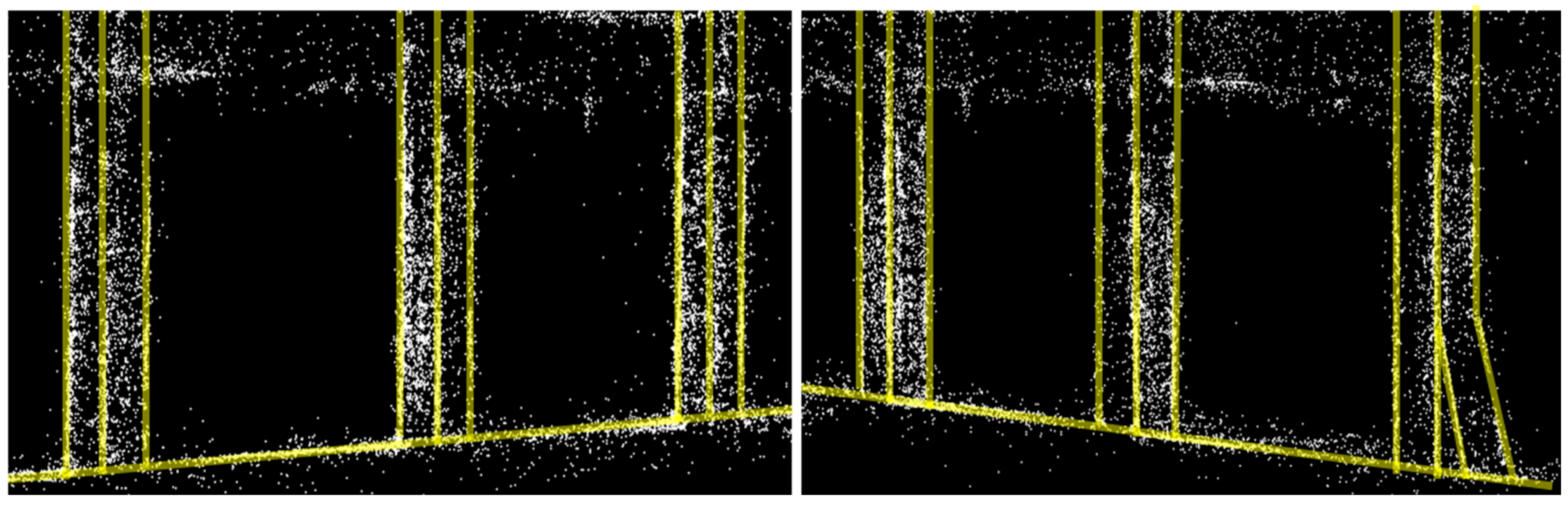
We found that the LDSO’s density is largely influenced by the number of points involved in the windowed optimization module (Figure 1b), because more points accepted by the windowed optimization module indicates more point depth values which are then converged, and therefore more points which can be reconstructed. We therefore increased the number of points involved in the windowed optimization module from 2000 to 3000 and ran before-and-after tests using a benchmark dataset, the results of which confirmed the density improvement resultant from our fine-tuning. We used the Technical University of Munich Monocular Visual Odometry (TUM Mono Vo) dataset, which is a widely used benchmark dataset in monocular VSLAM studies [58], for our test. The dataset comprises 50 videos from different sites, all of which are recorded by a closed loop [58]. We ran these datasets through both the original and tuned LDSOs and compared the total number of reconstructed points of the two resultant 3D point clouds (Figure 3).
Figure 3 illustrates examples from the test results (TUM Mono VO #39, #40, and #41), which allow for visual verification of the tuned LDSO’s capacity to reconstruct a much denser 3D point cloud than that produced by the original LDSO. Table 2 summarizes the detailed results of the entire test. As Table 2 demonstrates, the total number of reconstructed points significantly increased for all 50 videos when using the tuned LDSO, exhibiting an increase in the total number of reconstructed points of between 53% and 69%, and recording an average increase of 61.05%, with a standard deviation of merely 4.40% across all 50 videos. This low standard deviation is a clear indicator that the tuned LDSO can consistently improve the 3D point cloud density, without being affected by variations across given data (e.g., illumination and viewpoint variations) (Table 2).
3.3.2. More Robust Loop Closure
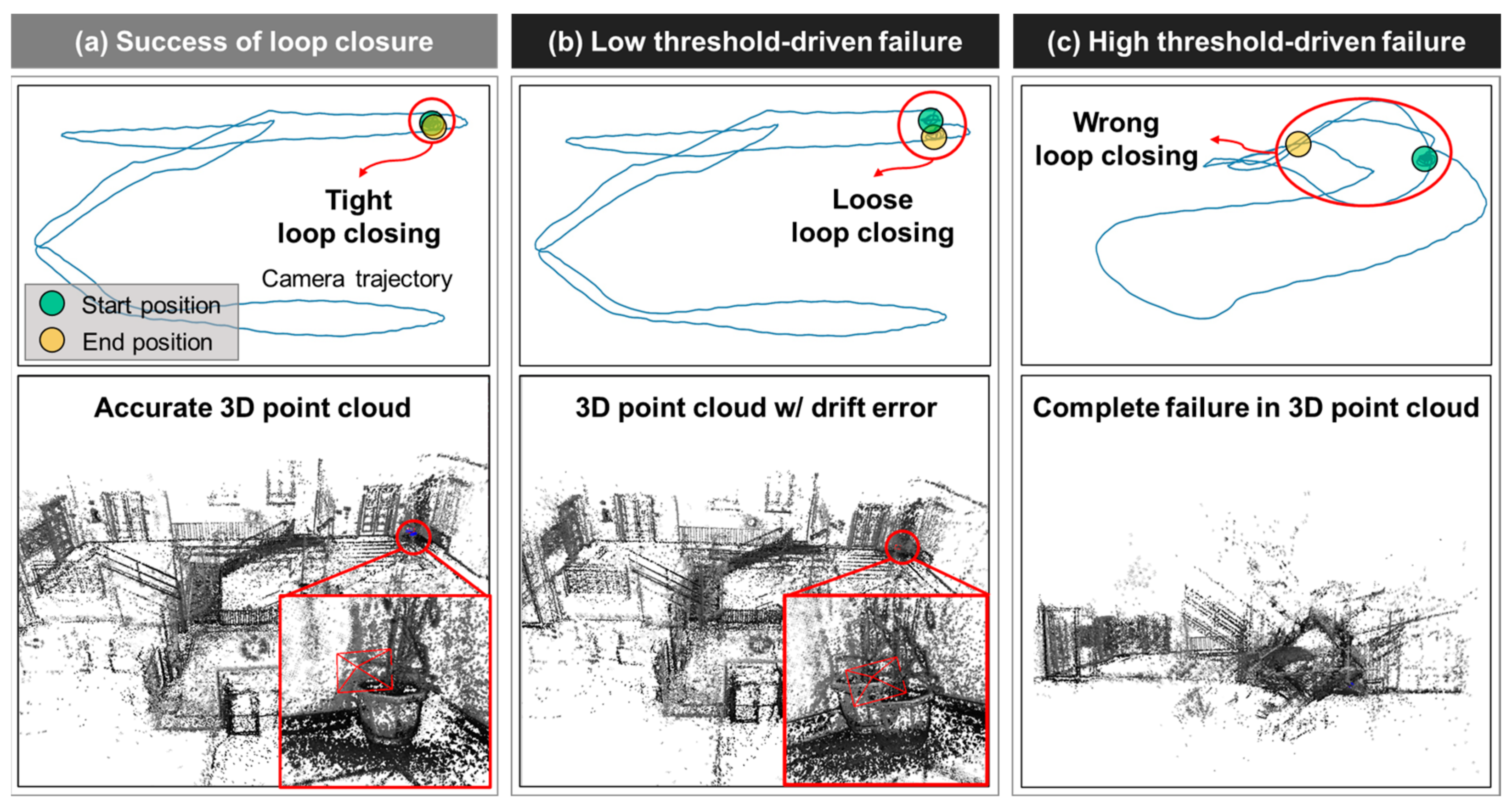
Because the original LDSO, as with conventional VSLAMs, estimates the camera’s 3D location and orientation frame by frame in a sequence, the errors from each frame are bound to accumulate, eventually resulting in inconsistencies that show up in the reconstructed 3D point cloud (Figure 4a,b). The original LDSO incorporates the loop closure module (Figure 1c) to diminish the inconsistency, but such drift errors are often observed in real-site applications under unpredictable conditions.
The main function of loop closure is tracking the camera’s trajectory and closing it, creating a complete loop when the camera returns to its starting position [53]. In the original LDSO, the validity of each loop candidate is heavily influenced by the quantitative condition of the ORB features of the two consecutive frames. That is, the candidate is accepted as a true loop, and the camera trajectory closed only if there are at least 10 matched features between the two frames. The threshold for feature matching was empirically set by the original authors but could, however, be too strict a standard for application to construction images, which tend to be highly complex and unstructured. A lower threshold for feature matching is highly likely to lead to fewer matched features and result in failed loop closures (Figure 4b). However, merely applying a higher threshold instead would not be an effective solution. Setting too high a threshold risks the module possibly closing the loop at an incorrect position, which can, in turn, lead to the complete failure of the 3D point cloud (Figure 4c).
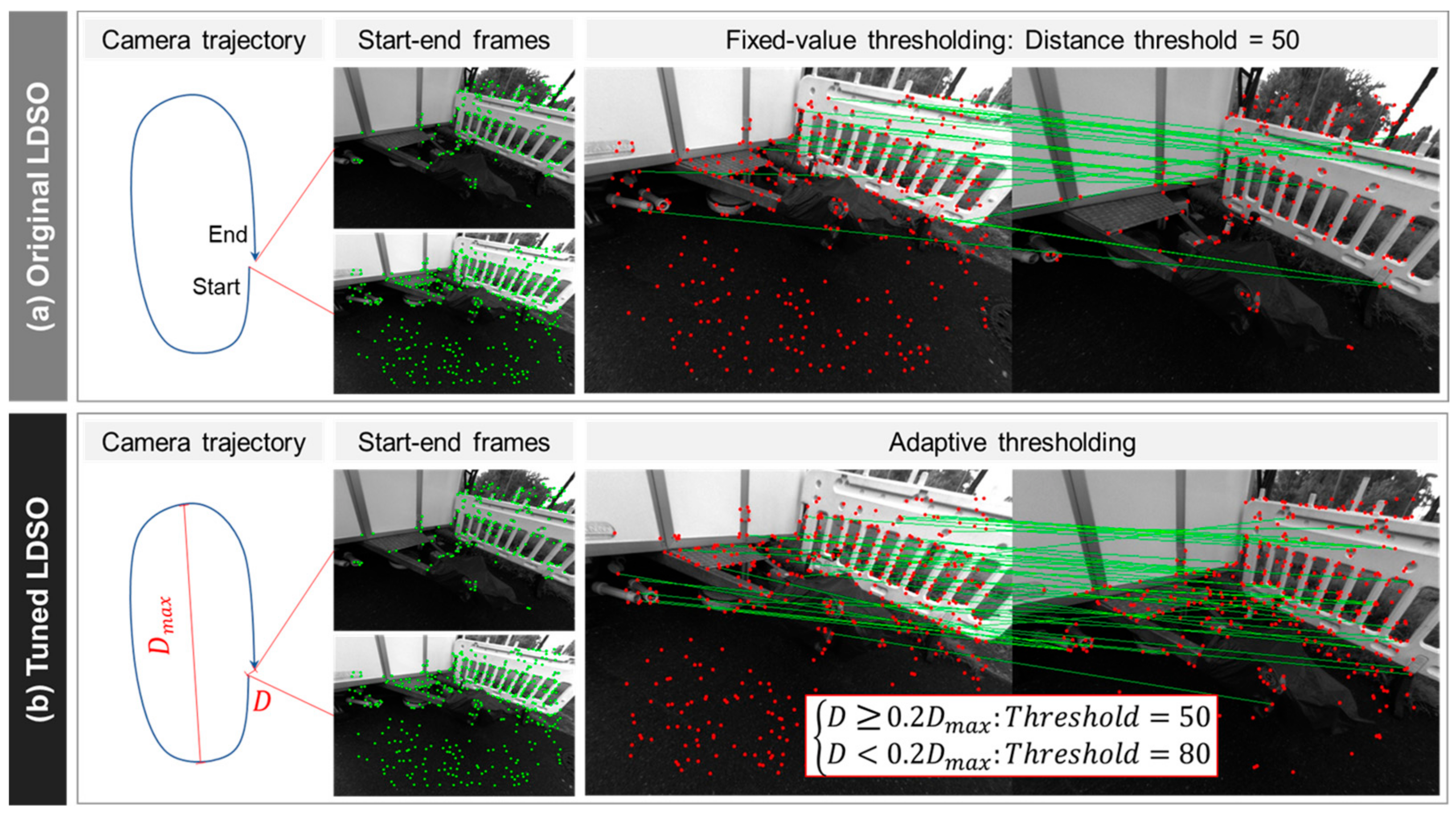
Instead of applying a fixed value for the feature matching threshold, we attempted to tune it by embedding an adaptive thresholding feature. Equation (1) denotes the adaptive thresholding feature for the ORB feature matching.
where = the distance between the starting and ending candidates’ locations; = the maximum distance between two arbitrary points along the camera’s trajectory; α = adjustable hyper-parameter.
The adaptive thresholding feature first measures the distance between the starting and ending candidates’ locations (denoted by D, Figure 5) and the maximum distance between two arbitrary points along the camera’s trajectory (denoted by, Figure 5). The adaptive thresholding feature applies different threshold values according to a comparison between D and (Equation (1)). When the starting and ending candidates are too disparately located—greater than or equal to α% of —the algorithm applies a low threshold for feature matching (50 matched features) in order to prevent the loop closure module from accepting unmatched starting–end candidates as a closed loop. Using the same principle, it applies a relatively high threshold for feature matching (80 matched features) when the D is less than α% of . Herein, we intended to set α as an adjustable hyper-parameter which can be flexibly customized in accordance with a target site’s layout. For the time being, we set the default value of α through an experiment with the TUM Mono VO dataset: we investigated average drift error (distance) between starting–end candidates’ locations without the loop closure module and set α = 20 as a moderate value for common cases since the drift error usually falls into the range of 20% of .
In a test using the TUM Mono VO dataset, we observed a significant improvement in loop closure. The original LDSO demonstrated a success rate of merely 14% for the 50 TUM Mono VO videos, whereas the tuned LDSO recorded a success rate of 74% (Table 3).
The tuned LDSO failed during the loop closure of several videos, and in analyzing the failures, we determined that they were due to challenging imaging conditions, such as (i) environments lacking sufficient objects from which to derive enough feature points and (ii) frequent overlap of the camera’s receptive field. However, it is noted that the TUM Mono VO dataset is meant to consist of videos depicting highly challenging conditions, which are not common even in real construction fields. Additionally, because camera trajectory overlap can be easily avoided in practice, this factor would not be too impactful in real field applications.
4. Field Test and Performance Evaluation
We tested the tuned LDSO at a real construction site, where we conducted the proof of concept for our near real-time 3D reconstruction and evaluated the quality of the 3D point cloud in detail at both object and site scales. This section describes the test setting and the evaluation criteria and metrics, and lastly presents the test results and their implications.
4.1. Test Setting
The field test took place at a building renovation site, located at Ann Arbor, Michigan, U.S., where all mechanical, electrical, and plumbing elements had been removed, and only structural elements (e.g., slabs, columns, and walls) remained (Figure 6a). We scanned a whole floor (50 m × 20 m) with a camera-mounted hardhat (Figure 6b) in one closed loop (Figure 6c), which took around 10 min. Meanwhile, the tuned LDSO reconstructed the 3D point cloud of the floor after viewing the site only once. A monocular camera (UI-3241LE, IDS [59]) was employed, and camera calibration was completed prior to site scanning to remove radial distortion as well as to refine its intrinsic parameters, such as focal length and principal point.
4.2. Evaluation Criteria
We evaluated the quality of the reconstructed 3D point cloud at both object and site scales and measured the tuned LDSO’s overall running speed. At the object scale, we considered two evaluation criteria: shape accuracy and point density. For the site-scale evaluation, we measured the cloud-to-cloud distance between the reconstructed 3D point cloud and the ground truth model to determine overall accuracy. In both object- and site-scale evaluations, a Terrestrial Laser Scanner (TLS, Focuss S350, FARO [60]) was employed and the laser-scanned 3D point cloud with ± 1 mm error was used as the ground truth.
4.3. Evaluation Metrics
We evaluated at object scale using the following metrics: (i) Aspect Ratio Error (ARE, %) for shape accuracy and (ii) Average # of Points Per Unit Surface Area (APS, EA/m2) for point density. Meanwhile, at the site scale, we used the Hausdorff Distance (cm) to measure cloud-to-cloud distance. Lastly, we measured the tuned LDSO’s Frames Per Second (FPS, f/s) to evaluate its overall running speed.
Aspect Ratio Error (ARE, %) for shape accuracy at object scale: To assess the shape accuracy of a reconstructed object (e.g., column), we measured its AREs for all the three dimensions (i.e., XY, YZ, and XZ planes). ARE is the percentage error compared to the ground truth aspect ratio (Equation (2)), and was first introduced in a previous study [41] as a metric used to assess the shape accuracy of 3D point clouds at object scale.
where = aspect ratio error for X-Y dimension; = aspect ratio error for Y-Z dimension; = aspect ratio error for X-Z dimension; = ground truth length on X-axis; = ground truth length on Y-axis; = ground truth length on Z-axis; = reconstructed length on X-axis; = reconstructed length on Y-axis; = reconstructed length on Z-axis.
- The Average # of Points Per Unit Surface Area (APS, EA/m2) for point density at object scale: We measured a reconstructed object’s (e.g., column) APS to assess its point density. The point density per unit surface area (m2) is first calculated for each surface of the element; the APS of the object then denotes the average of the point density values across all the object’s surfaces (Equation (3)).where = the # of points on the ith surface; = the area of ith surface (unit: m2); m = the total # of surfaces.
- Hausdorff Distance (cm) for cloud-to-cloud distance at site scale: To evaluate the reconstructed 3D point cloud’s overall discrepancy from the ground truth model, we measured the intervening Hausdorff Distance, which is the most widely applied metric in evaluating the distance between two 3D point clouds [21,33]. The Hausdorff Distance is the average value of the nearest distances between the ground truth model and the reconstructed 3D point cloud (Equation (3)). Each point in the ground truth model is matched to its nearest point in the reconstructed 3D point cloud and the distance between the two is measured. The Hausdorff Distance is the average value of all these nearest distances, which represents the overall discrepancy of the reconstructed 3D point cloud to its ground truth (Equation (4)).where = the ith point of ground truth 3D point cloud; = points of reconstructed 3D point cloud; m = the total # of points of ground truth 3D point cloud.
- Frames Per Second (FPS, f/s) for overall running speed: A camera streams a digital image to a computer every 0.033 s, a rate totaling 30 FPS. The near real-time 3D reconstruction thus requires an FPS of around 30. We measured the tuned LDSO’s FPS during the field test and compared it to the real-time standard, thereby demonstrating its potential for use in the near real-time 3D reconstruction of a construction site.
4.4. Object-Scale Evaluation and Result
We evaluated the shape accuracy (i.e., ARE, %) and point density (i.e., APS, EA/m2) of the test site’s 15 reconstructed concrete columns (Figure 7). As shown in Table 4, the reconstructed 3D point cloud recorded low AREs (%) for all the XY, XZ, and YZ planes along with high APS (EA/m2): on average, the reconstructed 3D point cloud achieved 1.55%, 2.40%, and 2.61% AREs for XY, XZ, and YZ planes, respectively, along with an APS (EA/m2) of 1286 (Table 4).
Our results indicate that the tuned LDSO can produce a 3D point cloud at competitive shape accuracy (i.e., low ARE) compared with current technologies; our tuned LDSO achieved an overall ARE of 2.19% (averaged across all the three planes), which is competitive with that reported for an SfM-based 3D point cloud in a previous study (3.53% ARE [41]). That the tuned LDSO’s AREs averaged less than 3% across all three planes indicates that it can model objects in minute detail and at high shape accuracy for all dimensions.
The tuned LDSO also demonstrated its ability to produce a sufficiently dense 3D point cloud for use in semantic inference (e.g., object detection). It satisfied the minimum density standard, suggested by Rebolj et al. [57], of 3D point clouds used for construction object detection. According to this study, a 3D point cloud of an object must have an APS of more than 530 for accurate automated object detection [57]. Our LDSO surpassed the minimum density standard with a huge margin of more than 200% that is required (1247 APS ≥ 530 APS) (Table 4).
Last but not least, in the realm of object-scale reconstruction, the tuned LDSO demonstrated its capability to model objects at low variance, with coefficients for all ARE variations (i.e., the ratio of standard deviation to average) across XY, XZ, and YZ planes of less than one, and a similarly low APS. The result proves that the tuned LDSO is capable of modeling objects at low variance against potentially variable imaging conditions (e.g., different viewpoint).
4.5. Site-Scale Evaluation and Result
The reconstructed 3D point cloud also shows promise at site-scale evaluation. The 3D point cloud (Figure 8a) was superimposed with the laser-scanned ground truth model (Figure 8b) through the Iterative Closet Point (ICP) algorithm, which is an algorithm widely used for aligning two sets of 3D point clouds. Then, the Hausdorff Distance between the reconstructed 3D point cloud and laser-scanned ground truth model was calculated (Equation (3)) within the composite 3D point cloud (Figure 8c). The resulting Hausdorff Distance for the reconstructed 3D point cloud was 17.3 cm, compared to the laser-scanned ground truth.
The Hausdorff Distance achieved by the tuned LDSO is lower than that of several types of commercial SfM-based 3D reconstruction software (19 cm [21] and 21 cm [33]). However, our LDSO was unable to reach the Hausdorff Distance achieved by state-of-the-art SfM-based 3D reconstruction in a previous study (5 cm [21]). Regardless, the tuned LDSO has an advantage over SfM-based 3D reconstruction in that it can generate a 3D point cloud in near real-time at a moderate level of accuracy, something no SfM-based 3D reconstruction technology is currently capable of. This has significant potential to impact time-critical construction monitoring tasks, as detailed in the following discussion section (Section 5).
4.6. Overall Running Speed
The tuned LDSO demonstrated its near real-time operation during the field test, with 24 FPS overall (real-time standard = 30 FPS). While scanning the 50 m × 20 m test site, it processed all input sequences, showing little lag time throughout computation, including during visualization. That is, the result could be visualized while scanning the site simultaneously. The tuned LDSO took merely 12 min and 34 s to complete the entire process, whereas laser scanning took seven hours. The site scanning took around 10 min, and the tuned LDSO completed the 3D reconstruction of the site after another 2 min and 34 s.
5. Discussion: Near Real-Time 3D Reconstruction for Time-Critical Construction Monitoring Tasks
The tuned LDSO allows for the 3D reconstruction of a construction site—with minimal hardware installation and without requiring expertise in site imaging. Construction professionals can conduct 3D reconstruction by simply surveying the region of interest with a camera-mounted hardhat, making a closed loop. This can even be accomplished while they carry out their regular tasks. In a field test, the tuned LDSO demonstrated its near real-time operation while producing a high-quality 3D point cloud comparable to that of an SfM-based 3D reconstruction. The convenience, rapidity, and quality of the tuned LDSO indicate its far-reaching potential to facilitate 3D reconstruction for time-critical construction monitoring tasks.
5.1. Online 3D Reconstruction: Simultaneous Scanning and Visualization
One concrete advantage of the tuned LDSO is its online 3D reconstruction, wherein site scanning feedback becomes immediately available due to rapid 3D reconstruction and visualization. The existing 3D reconstruction methods, including those based on LiDAR and photogrammetry, only function offline. In other words, the process for these methods takes two steps: a complete on-site scanning, either laser scanning or site imaging, is conducted first, and in-office 3D reconstruction and visualization then follow. The practical concern here is that site scanning often needs to be redone due to misalignment among resultant 3D point clouds or missing site details in the images utilized for 3D reconstruction. Using existing methods, there is no way to pre-qualify the scanned data before examining the result of the 3D reconstruction; the long run-time of existing 3D reconstruction methods disallows this. Note that the TLS-based 3D reconstruction took around seven hours total, including the time necessary to complete visualization for the test site (50 m × 20 m). As noted by many previous studies [3,12,18,35], SfM-based 3D reconstruction generally has an FPS of less than 0.01, which is entirely insufficient for near real-time 3D reconstruction and thus for immediate site scanning feedback.
The tuned LDSO, on the other hand, can be used online, such that site scanning updates at the moment in accordance with the resultant 3D point cloud. A worker can directly check the quality of the 3D point cloud while scanning the site. If a mismatch or a sparsity is found in the 3D point cloud, the worker can easily correct it by simply re-scanning the region and confirming the quality of the 3D point cloud. As such, the tuned LDSO, with its near real-time operation, can contribute to making the overall process of 3D reconstruction for a construction site more convenient, efficient, and rapid. These advantages would in turn, lead to better facilitation of 3D reconstruction in time-critical construction monitoring tasks, such as safety and progress monitoring.
5.2. Near Real-Time 3D Reconstruction for Regular and Timely Monitoring
The core function of progress monitoring lies in identifying discrepancies between as-built and as-planned progress as soon as possible and taking timely corrective actions, thereby minimizing unexpected costs due to delays and reworks. To this end, regular and timely site modeling is of vital importance; however, the existing methods—such as those based on TLS or SfM—exhibit excessive run times, which limit their utility for effective progress monitoring.
As a corrective strategy, our tuned LDSO presents an effective solution for progress monitoring, while complementing the existing methods. The tuned LDSO is easy to apply at a minimal cost and is also capable of as-built modeling (i.e., 3D reconstruction) in near real-time. A project manager (or a field worker) can easily scan their jobsite with a camera-mounted hardhat and acquire the as-built model of the site shortly thereafter. In the case of a large-scale project, scanning can be completed by multiple agents, and the as-built modeling of the site can be created simply by registering the resultant multiple 3D point clouds into one composite model. Therefore, the tuned LDSO presents a convenient method which can help a project manager with regular and timely progress monitoring. More importantly, the near real-time 3D reconstruction can provide said project manager with the data necessary to identify and control discrepancies between as-built and as-planned progresses at the earliest opportunity.
The near real-time 3D reconstruction along with other computer vision tasks, such as object detection, can enhance onsite safety monitoring. Take, for example, the vision-based proximity monitoring applications that have been exercised in 2D space. It can be readily expanded to 3D proximity detection coupled with near real-time 3D reconstruction. While capturing a construction scene, 2D object detection and 3D reconstruction can be completed simultaneously, which enables us to have the full 3D coordinates of objects of interest, making it possible to estimate the target distance (i.e., proximity) in 3D space. For the other safety applications that require the missing third coordinates, the same principle can be applied.
5.3. Improvement Point toward Real Field Applications: Real-Time Data Transmission
The quality and speed of the network connection between the imaging device (or devices) and computing server need to be further investigated prior to the tuned LDSO’s use in real-field applications. The tuned LDSO uses a camera-mounted hardhat to generate image inputs, which then must be streamed in real-time to either a local or a web-based computing server. Therefore, it is important to ensure rapid data transmission between imaging devices and the computing server. Leveraging a 5G wireless network and Internet of Things (IoT) cloud platform may be a promising solution to this potential problem. The 5G wireless network would support real-time data transmission at a data transfer rate of several gigabytes per second. With such a high-speed network connection, an IoT cloud platform could, in turn connect multiple imaging devices to a cloud server, thereby supporting the wireless, near real-time operation of 3D reconstruction at real construction sites.
The application scope of the proposed tuned LDSO can be further expanded with the semantic modeling of a 3D point cloud. Digital twin or smart construction needs to model the 3D real world in a digital space, which requires not only accurate 3D reconstruction in real time but also semantic information of reconstructed entities (e.g., class labels). When a 3D point cloud comes with such semantic information (e.g., class labels), site monitoring tasks such as progress monitoring and hazard detection can be more automated in a digital space. For the semantic modeling of a 3D point cloud, a 2D image-based deep neural network for semantic segmentation can be considered to be integrated with the proposed tuned LDSO.
6. Conclusions
3D reconstruction has the potential to automate construction monitoring tasks. However, the primary research focus of this area has thus far been improving the quality of 3D point clouds, with little attention paid to achieving the near real-time operation necessitated by time-critical monitoring tasks such as regular progress monitoring or hazard detection. As a corrective strategy, this paper presented an enhanced LDSO-based 3D reconstruction technique, which is capable of simultaneously achieving near real-time operation while creating a quality 3D point cloud. During validation using the TUM Mono VO dataset, the proposed method demonstrated notable improvements in point density and loop closure robustness: compared to the original LDSO, the density was improved by 61%, while the loop closure success rate improved from 14% to 74%. Further, in a field test, our method exhibited near real-time operation while creating a quality 3D point cloud comparable to that of the existing 3D reconstruction method (i.e., SfM). While the existing 3D reconstruction methods, such as those based on terrestrial LiDAR or SfM do not allow near real-time 3D reconstruction due to the significant amount of time required for site scanning and data processing, the proposed method provides a potentially more accessible 3D reconstruction with near real-time visualization. It will allow project managers to monitor their ongoing jobsites in a more convenient, efficient, and timely manner.
Author Contributions
Conceptualization, Z.L., D.K. and X.A.; methodology, Z.L., S.L. and X.A.; software, Z.L., L.Z. and M.L.; validation, Z.L., D.K. and L.Z.; formal analysis, Z.L., D.K. and L.Z.; investigation, Z.L., D.K. and L.Z.; resources, Z.L. and D.K.; data curation, Z.L. and D.K.; writing—original draft preparation, Z.L., D.K. and L.Z.; writing—review and editing, S.L., X.A. and M.L.; visualization, Z.L. and L.Z.; supervision, S.L. and X.A.; funding acquisition, Z.L. and X.A. All authors have read and agreed to the published version of the manuscript.
Funding
This research was funded by the China Scholarship Council (CSC) during a visit of Zuguang Liu to Michigan and State Key Laboratory of Hydroscience and Engineering, Tsinghua University, grant number 2021-KY-01 (Research on Key Technologies of Smart Water Platform Based on Hydrology and Hydrodynamic Model).
Data Availability Statement
All data, models, or codes that support the findings of this study are available from the corresponding author upon reasonable request. The data are not publicly available due to site privacy.
Acknowledgments
We wish to thank Barton Malow Co. for their considerate assistance in field testing.
Conflicts of Interest
The authors declare no conflict of interest.
References
- Brilakis, I.; Fathi, H.; Rashidi, A. Progressive 3D reconstruction of infrastructure with videogrammetry. Autom. Constr. 2011, 20, 884–895. [Google Scholar] [CrossRef]
- Ma, Z.; Liu, S. A review of 3D reconstruction techniques in civil engineering and their applications. Adv. Eng. Inform. 2018, 37, 163–174. [Google Scholar] [CrossRef]
- Fathi, H.; Dai, F.; Lourakis, M. Automated as-built 3D reconstruction of civil infrastructure using computer vision: Achievements, opportunities, and challenges. Adv. Eng. Inform. 2015, 29, 149–161. [Google Scholar] [CrossRef]
- McCoy, A.P.; Golparvar-Fard, M.; Rigby, E.T. Reducing Barriers to Remote Project Planning: Comparison of Low-Tech Site Capture Approaches and Image-Based 3D Reconstruction. J. Arch. Eng. 2014, 20, 05013002. [Google Scholar] [CrossRef]
- Sung, C.; Kim, P.Y. 3D terrain reconstruction of construction sites using a stereo camera. Autom. Constr. 2016, 64, 65–77. [Google Scholar] [CrossRef]
- Siebert, S.; Teizer, J. Mobile 3D mapping for surveying earthwork projects using an Unmanned Aerial Vehicle (UAV) system. Autom. Constr. 2014, 41, 1–14. [Google Scholar] [CrossRef]
- Pučko, Z.; Šuman, N.; Rebolj, D. Automated continuous construction progress monitoring using multiple workplace real time 3D scans. Adv. Eng. Inform. 2018, 38, 27–40. [Google Scholar] [CrossRef]
- Han, K.; Degol, J.; Golparvar-Fard, M. Geometry- and Appearance-Based Reasoning of Construction Progress Monitoring. J. Constr. Eng. Manag. 2018, 144, 04017110. [Google Scholar] [CrossRef]
- Puri, N.; Turkan, Y. Bridge construction progress monitoring using lidar and 4D design models. Autom. Constr. 2020, 109, 102961. [Google Scholar] [CrossRef]
- Puri, Y.; Nisha, T. A Review of Technology Supplemented Progress Monitoring Techniques for Transportation Construction Projects. In Construction Research Congress 2018; American Society of Civil Engineers: Reston, VA, USA, 2018; pp. 512–521. [Google Scholar]
- Golparvar-Fard, M.; Peña-Mora, F.; Savarese, S. D4AR-A 4-Dimensional Augmented Reality Model for Automating Construction Progress Monitoring Data Collection, Processing and Communication. J. Inf. Technol. Constr. 2009, 14, 129–153. [Google Scholar]
- Han, K.K.; Golparvar-Fard, M. Appearance-based material classification for monitoring of operation-level construction progress using 4D BIM and site photologs. Autom. Constr. 2015, 53, 44–57. [Google Scholar] [CrossRef]
- Lin, J.J.; Lee, J.Y.; Golparvar-Fard, M. Exploring the Potential of Image-Based 3D Geometry and Appearance Reasoning for Automated Construction Progress Monitoring. In Computing in Civil Engineering 2019; American Society of Civil Engineers: Reston, VA, USA, 2019; pp. 162–170. [Google Scholar] [CrossRef]
- Gholizadeh, P.; Behzad, E.; Memarian, B. Monitoring Physical Progress of Indoor Buildings Using Mobile and Terrestrial Point Clouds. In Construction Research Congress 2018; ASCE: Reston, VA, USA, 2018; pp. 602–611. [Google Scholar]
- Tang, P.; Huber, D.; Akinci, B. Characterization of Laser Scanners and Algorithms for Detecting Flatness Defects on Concrete Surfaces. J. Comput. Civ. Eng. 2011, 25, 31–42. [Google Scholar] [CrossRef]
- Olsen, M.J.; Kuester, F.; Chang, B.J.; Hutchinson, T.C. Terrestrial Laser Scanning-Based Structural Damage Assessment. J. Comput. Civ. Eng. 2010, 24, 264–272. [Google Scholar] [CrossRef]
- Rabah, M.; Elhattab, A.; Fayad, A. Automatic concrete cracks detection and mapping of terrestrial laser scan data. NRIAG J. Astron. Geophys. 2013, 2, 250–255. [Google Scholar] [CrossRef]
- Khaloo, A.; Lattanzi, D.; Cunningham, K.; Dell’Andrea, R.; Riley, M. Unmanned aerial vehicle inspection of the Placer River Trail Bridge through image-based 3D modelling. Struct. Infrastruct. Eng. 2018, 14, 124–136. [Google Scholar] [CrossRef]
- Liu, Y.-F.; Cho, S.; Spencer, B.F.; Fan, J.-S. Concrete Crack Assessment Using Digital Image Processing and 3D Scene Reconstruction. J. Comput. Civ. Eng. 2016, 30, 04014124. [Google Scholar] [CrossRef]
- Torok, M.M.; Golparvar-Fard, M.; Kochersberger, K.B. Image-Based Automated 3D Crack Detection for Post-disaster Building Assessment. J. Comput. Civ. Eng. 2014, 28, A4014004. [Google Scholar] [CrossRef]
- Ghahremani, K.; Khaloo, A.; Mohamadi, S.; Lattanzi, D. Damage Detection and Finite-Element Model Updating of Structural Components through Point Cloud Analysis. J. Aerosp. Eng. 2018, 31, 04018068. [Google Scholar] [CrossRef]
- Isailović, D.; Stojanovic, V.; Trapp, M.; Richter, R.; Hajdin, R.; Döllner, J. Bridge damage: Detection, IFC-based semantic enrichment and visualization. Autom. Constr. 2020, 112, 103088. [Google Scholar] [CrossRef]
- Xiong, X.; Adan, A.; Akinci, B.; Huber, D. Automatic creation of semantically rich 3D building models from laser scanner data. Autom. Constr. 2013, 31, 325–337. [Google Scholar] [CrossRef] [Green Version]
- Valero, E.; Adán, A.; Bosché, F. Semantic 3D Reconstruction of Furnished Interiors Using Laser Scanning and RFID Technology. J. Comput. Civ. Eng. 2016, 30, 04015053. [Google Scholar] [CrossRef]
- Uslu, B.; Golparvar-Fard, M.; de la Garza, J.M. Image-Based 3D Reconstruction and Recognition for Enhanced Highway Condition Assessment. Comput. Civ. Eng. 2011, 67–76. [Google Scholar] [CrossRef]
- Xuehui, A.; Li, Z.; Zuguang, L.; Chengzhi, W.; Pengfei, L.; Zhiwei, L. Dataset and benchmark for detecting moving objects in construction sites. Autom. Constr. 2021, 122, 103482. [Google Scholar] [CrossRef]
- Fang, Y.; Cho, Y.K.; Chen, J. A framework for real-time pro-active safety assistance for mobile crane lifting operations. Autom. Constr. 2016, 72, 367–379. [Google Scholar] [CrossRef]
- Nahangi, M.; Yeung, J.; Haas, C.T.; Walbridge, S.; West, J. Automated assembly discrepancy feedback using 3D imaging and forward kinematics. Autom. Constr. 2015, 56, 36–46. [Google Scholar] [CrossRef]
- Rodríguez-Gonzálvez, P.; Rodríguez-Martín, M.; Ramos, L.F.; González-Aguilera, D. 3D reconstruction methods and quality assessment for visual inspection of welds. Autom. Constr. 2017, 79, 49–58. [Google Scholar] [CrossRef]
- Wang, Q. Automatic checks from 3D point cloud data for safety regulation compliance for scaffold work platforms. Autom. Constr. 2019, 104, 38–51. [Google Scholar] [CrossRef]
- Jog, G.M.; Koch, C.; Golparvar-Fard, M.; Brilakis, I. Pothole Properties Measurement through Visual 2D Recognition and 3D Reconstruction. Comput. Civ. Eng. 2012, 2012, 553–560. [Google Scholar]
- Fard, M.G.; Pena-Mora, F. Application of visualization techniques for construction progress monitoring. In Proceedings of the International Workshop on Computing in Civil Engineering 2007, Pittsburgh, PA, USA, 24–27 July 2007; pp. 216–223. [Google Scholar]
- Khaloo, A.; Lattanzi, D. Hierarchical Dense Structure-from-Motion Reconstructions for Infrastructure Condition Assessment. J. Comput. Civ. Eng. 2017, 31, 04016047. [Google Scholar] [CrossRef]
- Popescu, C.; Täljsten, B.; Blanksvärd, T.; Elfgren, L. 3D reconstruction of existing concrete bridges using optical methods. Struct. Infrastruct. Eng. 2019, 15, 912–924. [Google Scholar] [CrossRef]
- Rashidi, A.; Dai, F.; Brilakis, I.; Vela, P. Optimized selection of key frames for monocular videogrammetric surveying of civil infrastructure. Adv. Eng. Inform. 2013, 27, 270–282. [Google Scholar] [CrossRef]
- Dai, F.; Rashidi, A.; Brilakis, I.; Vela, P. Comparison of Image-Based and Time-of-Flight-Based Technologies for Three-Dimensional Reconstruction of Infrastructure. J. Constr. Eng. Manag. 2013, 139, 69–79. [Google Scholar] [CrossRef]
- Gao, X.; Wang, R.; Demmel, N.; Cremers, D. LDSO: Direct Sparse Odometry with Loop Closure. In Proceedings of the 2018 IEEE/RSJ International Conference on Intelligent Robots and Systems (IROS), Madrid, Spain, 1–5 October 2018; pp. 2198–2204. [Google Scholar] [CrossRef]
- Jaselskis, E.J.; Gao, Z.; Walters, R.C. Improving Transportation Projects Using Laser Scanning. J. Constr. Eng. Manag. 2005, 131, 377–384. [Google Scholar] [CrossRef]
- Oskouie, P.; Becerik-Gerber, B.; Soibelman, L. Automated measurement of highway retaining wall displacements using terrestrial laser scanners. Autom. Constr. 2016, 65, 86–101. [Google Scholar] [CrossRef]
- Zhu, Z.; Brilakis, I. Comparison of Civil Infrastructure Optical-Based Spatial Data Acquisition Techniques. In Computing in Civil Engineering (2007); ASCE: Reston, VA, USA, 2007; pp. 737–744. [Google Scholar] [CrossRef]
- Golparvar-Fard, M.; Bohn, J.; Teizer, J.; Savarese, S.; Peña-Mora, F. Evaluation of image-based modeling and laser scanning accuracy for emerging automated performance monitoring techniques. Autom. Constr. 2011, 20, 1143–1155. [Google Scholar] [CrossRef]
- Schonberger, J.L.; Frahm, J.M. Structure-from-Motion Revisited. In Proceedings of the 2016 IEEE Conference on Computer Vision and Pattern Recognition, Las Vegas, NV, USA, 27–30 June 2016; pp. 4104–4113. [Google Scholar]
- Saputra, M.R.U.; Markham, A.; Trigoni, N. Visual SLAM and Structure from Motion in Dynamic Environments: A survey. ACM Comput. Surv. 2018, 51, 1–36. [Google Scholar] [CrossRef]
- Maalek, R.; Ruwanpura, J.; Ranaweera, K. Evaluation of the State-of-the-Art Automated Construction Progress Monitoring and Control Systems. In Construction Research Congress 2014; American Society of Civil Engineers: Reston, VA, USA, 2014; pp. 1023–1032. [Google Scholar] [CrossRef]
- Tang, P.; Huber, D.; Akinci, B.; Lipman, R.; Lytle, A. Automatic reconstruction of as-built building information models from laser-scanned point clouds: A review of related techniques. Autom. Constr. 2010, 19, 829–843. [Google Scholar] [CrossRef]
- Choi, J. Detecting and Classifying Cranes Using Camera-Equipped UAVs for Monitoring Crane-Related Safety Hazards. In Computing in Civil Engineering 2017; ASCE: Reston, VA, USA, 2017; pp. 442–449. [Google Scholar]
- Kim, H.; Kim, K.; Kim, H. Data-driven scene parsing method for recognizing construction site objects in the whole image. Autom. Constr. 2016, 71, 271–282. [Google Scholar] [CrossRef]
- Rublee, E.; Rabaud, V.; Konolige, K.; Bradski, G. ORB: An efficient alternative to SIFT or SURF. In Proceedings of the IEEE International Conference on Computer Vision, Barcelona, Spain, 6–13 November 2011; pp. 2564–2571. [Google Scholar] [CrossRef]
- Agarwal, S.; Snavely, N.; Simon, I.; Seitz, S.; Szeliski, R. Building Rome in a Day. In Proceedings of the 2009 IEEE 12th International Conference on Computer Vision, Kyoto, Japan, 27 September–4 October 2009; pp. 72–79. [Google Scholar] [CrossRef]
- Gherardi, R.; Farenzena, M.; Fusiello, A. Improving the Efficiency of Hierarchical Structure-and-Motion. In Proceedings of the 2010 IEEE Computer Society Conference on Computer Vision and Pattern Recognition, San Francisco, CA, USA, 13–18 June 2010; pp. 1594–1600. [Google Scholar]
- Crandall, D.; Owens, A.; Snavely, N.; Huttenlocher, D. Discrete-continuous optimization for large-scale structure from motion. In Proceedings of the CVPR 2011, Colorado Springs, CO, USA, 20–25 June 2011; pp. 3001–3008. [Google Scholar] [CrossRef]
- Engel, J.; Koltun, V.; Cremers, D. Direct Sparse Odometry. IEEE Trans. Pattern Anal. Mach. Intell. 2018, 40, 611–625. [Google Scholar] [CrossRef]
- Mur-Artal, R.; Montiel, J.M.M.; Tardos, J.D. ORB-SLAM: A Versatile and Accurate Monocular SLAM System. IEEE Trans. Robot. 2015, 31, 1147–1163. [Google Scholar] [CrossRef]
- Rosten, E.; Drummond, T. Machine Learning for High-Speed Corner Detection. In Proceedings of the Computer Vision–ECCV 2006: 9th European Conference on Computer Vision, Graz, Austria, 7–13 May 2006; pp. 430–443. [Google Scholar]
- Gálvez-López, D.; Tardos, J.D. Bags of Binary Words for Fast Place Recognition in Image Sequences. IEEE Trans. Robot. 2012, 28, 1188–1197. [Google Scholar] [CrossRef]
- Kümmerle, R.; Grisetti, G.; Strasdat, H.; Konolige, K.; Burgard, W. G2o: A General Framework for Graph Optimization. In Proceedings of the 2011 IEEE International Conference on Robotics and Automation, Shanghai, China, 9–13 May 2011; pp. 3607–3613. [Google Scholar]
- Rebolj, D.; Pučko, Z.; Babič, N.Č.; Bizjak, M.; Mongus, D. Point cloud quality requirements for Scan-vs-BIM based automated construction progress monitoring. Autom. Constr. 2017, 84, 323–334. [Google Scholar] [CrossRef]
- Engel, J.; Usenko, V.; Cremers, D. A Photometrically Calibrated Benchmark For Monocular Visual Odometry. arXiv 2016, arXiv:1607.02555. [Google Scholar]
- IDS Products. Available online: https://en.ids-imaging.com/our-corporate-culture.html (accessed on 9 November 2022).
- FARO. FARO® Focus Laser Scanners. Available online: https://www.faro.com/products/construction-bim/faro-focus/ (accessed on 9 November 2022).
Figure 1.
Framework of the original LDSO. Note: sliding window = a window to maintain five to seven key frames and 2000 matching points; active keyframes = 5 active keyframes in sliding window; marginalized keyframes = keyframes out of sliding window; active points = points of active keyframes in sliding window; marginalized points = points out of sliding window.

Figure 2.
Overall Workflow of the Tuned LDSO.

Figure 3.
Examples of reconstructed 3D point clouds on TUM Mono VO dataset: original vs. tuned LDSO.
Figure 3.
Examples of reconstructed 3D point clouds on TUM Mono VO dataset: original vs. tuned LDSO.

Figure 4.
Success and failure cases in loop closure and its resultant 3D point cloud.

Figure 5.
Loop closure module: (a) original LDSO and (b) tuned LDSO.

Figure 6.
Test setting: site footages and camera set-up.

Figure 7.
Reconstructed 3D point cloud of 15 concrete columns.

Figure 8.
Registration of the tuned LDSO’s 3D point cloud to laser-scanned ground truth.


Table 1.
The list of literature reviewed.
| Device | Data Processing Approach | Applications | Limitations |
|---|---|---|---|
| Terrestrial LiDAR | Reconstruct 3D digital model from 3D point cloud | ||
| Camera | SfM-based algorithm to extract 3D point cloud | ||
| VSLAM-based algorithm to extract 3D point cloud |
|
|
Table 2.
The number of reconstructed points: original vs. tuned LDSOs.
| Input Video | The Total # of Reconstructed Points | Percentage Increase (%) | Input Video | The Total Number of Reconstructed Points | Percentage Increase (%) | ||
|---|---|---|---|---|---|---|---|
| Original | Tuned | Original | Tuned | ||||
| 1 | 415,115 | 658,739 | 58.7% | 26 | 175,279 | 271,803 | 55.1% |
| 2 | 317,696 | 495,536 | 56.0% | 27 | 568,437 | 923,535 | 62.5% |
| 3 | 494,039 | 784,489 | 58.8% | 28 | 431,847 | 667,609 | 54.6% |
| 4 | 604,279 | 957,752 | 58.5% | 29 | 1,029,730 | 1,704,825 | 65.6% |
| 5 | 537,430 | 869,660 | 61.8% | 30 | 368,949 | 610,472 | 65.5% |
| 6 | 467,547 | 749,573 | 60.3% | 31 | 658,455 | 1,102,686 | 67.5% |
| 7 | 330,907 | 525,820 | 58.9% | 32 | 616,615 | 1,032,057 | 67.4% |
| 8 | 397,017 | 623,610 | 57.1% | 33 | 557,479 | 918,824 | 64.8% |
| 9 | 207,816 | 325,823 | 56.8% | 34 | 1,028,383 | 1,711,655 | 66.4% |
| 10 | 190,855 | 300,680 | 57.5% | 35 | 140,482 | 214,230 | 52.5% |
| 11 | 273,686 | 433,063 | 58.2% | 36 | 154,730 | 238,362 | 54.1% |
| 12 | 374,671 | 586,421 | 56.5% | 37 | 282,092 | 439,258 | 55.7% |
| 13 | 270,700 | 428,325 | 58.2% | 38 | 349,997 | 541,363 | 54.7% |
| 14 | 221,763 | 353,276 | 59.3% | 39 | 368,639 | 573,842 | 55.7% |
| 15 | 466,194 | 759,135 | 62.8% | 40 | 379,725 | 582,686 | 53.4% |
| 16 | 290,473 | 467,898 | 61.1% | 41 | 464,620 | 743,132 | 59.9% |
| 17 | 419,206 | 677,186 | 61.5% | 42 | 736,967 | 1,194,749 | 62.1% |
| 18 | 512,087 | 809,279 | 58.0% | 43 | 480,989 | 795,431 | 65.4% |
| 19 | 1,066,310 | 1,731,553 | 62.4% | 44 | 305,705 | 505,551 | 65.4% |
| 20 | 977,046 | 1,599,733 | 63.7% | 45 | 631,486 | 1,036,933 | 64.2% |
| 21 | 1,305,839 | 2,171,135 | 66.3% | 46 | 677,427 | 1,115,721 | 64.7% |
| 22 | 1,340,949 | 2,269,298 | 69.2% | 47 | 600,759 | 1,007,490 | 67.7% |
| 23 | 523,515 | 867,994 | 65.8% | 48 | 605,129 | 1,017,770 | 68.2% |
| 24 | 526,644 | 860,967 | 63.5% | 49 | 547,252 | 878,302 | 60.5% |
| 25 | 778,354 | 1,272,857 | 63.5% | 50 | 811,535 | 1,336,625 | 64.7% |
| The average of percentage increase (%) | 61.05% | ||||||
| The standard deviation of percentage increase (%) | 4.40% | ||||||
Table 3.
Loop closure test on TUM Mono VO dataset: original vs. tuned LDSO.
| LDSOs | Total Numcber of Videos | Total Number of Successful Loop Closure | Average Success Rate |
|---|---|---|---|
| Original | 50 | 7 | 14% |
| Tuned | 50 | 37 | 74% |
Table 4.
Shape accuracy and point density of 15 reconstructed concrete columns.
| Column # | Aspect Ratio Error (ARE, %) | Average # of Points/Unit Surface Area (APS, EA/m2) | ||
|---|---|---|---|---|
| XY | XZ | YZ | ||
| 1 | 0.71 | 4.16 | 4.9 | 722.72 |
| 2 | 1.87 | 2.76 | 0.83 | 1514.36 |
| 3 | 0.32 | 0.57 | 0.89 | 1801.47 |
| 4 | 0.15 | 3.4 | 3.25 | 687.45 |
| 5 | 1.64 | 1.46 | 0.16 | 2050.04 |
| 6 | 1.14 | 1.94 | 0.82 | 1475.80 |
| 7 | 1.55 | 7.78 | 9.45 | 1027.89 |
| 8 | 2.22 | 0.04 | 2.18 | 2367.51 |
| 9 | 0.41 | 0.18 | 0.6 | 1273.17 |
| 10 | 3.05 | 0.4 | 3.46 | 696. 47 |
| 11 | 3.72 | 2.95 | 0.88 | 1415.09 |
| 12 | 1.3 | 0.66 | 0.65 | 1242.82 |
| 13 | 2.04 | 4.8 | 2.86 | 896.63 |
| 14 | 3.23 | 2.12 | 5.42 | 1205.09 |
| 15 | 0.03 | 2.81 | 2.84 | 335.42 |
| Average | 1.56 | 2.40 | 2.61 | 1286.82 |
| Standard deviation | 1.11 | 2.02 | 2.42 | 529.82 |
| Coefficient variations | 0.71 | 0.84 | 0.92 | 0.41 |
Disclaimer/Publisher’s Note: The statements, opinions and data contained in all publications are solely those of the individual author(s) and contributor(s) and not of MDPI and/or the editor(s). MDPI and/or the editor(s) disclaim responsibility for any injury to people or property resulting from any ideas, methods, instructions or products referred to in the content. |
© 2023 by the authors. Licensee MDPI, Basel, Switzerland. This article is an open access article distributed under the terms and conditions of the Creative Commons Attribution (CC BY) license (https://creativecommons.org/licenses/by/4.0/).
Share and Cite
MDPI and ACS Style
Liu, Z.; Kim, D.; Lee, S.; Zhou, L.; An, X.; Liu, M. Near Real-Time 3D Reconstruction and Quality 3D Point Cloud for Time-Critical Construction Monitoring. Buildings 2023, 13, 464. https://doi.org/10.3390/buildings13020464
AMA Style
Liu Z, Kim D, Lee S, Zhou L, An X, Liu M. Near Real-Time 3D Reconstruction and Quality 3D Point Cloud for Time-Critical Construction Monitoring. Buildings. 2023; 13(2):464. https://doi.org/10.3390/buildings13020464
Chicago/Turabian StyleLiu, Zuguang, Daeho Kim, Sanghyun Lee, Li Zhou, Xuehui An, and Meiyin Liu. 2023. "Near Real-Time 3D Reconstruction and Quality 3D Point Cloud for Time-Critical Construction Monitoring" Buildings 13, no. 2: 464. https://doi.org/10.3390/buildings13020464
Note that from the first issue of 2016, this journal uses article numbers instead of page numbers. See further details here.