Measuring Emissions from a Demonstrator Heavy-Duty Diesel Vehicle under Real-World Conditions—Moving Forward to Euro VII

Abstract

The European Union (EU) has introduced since the early 1990s a series of progressively more stringent emission regulations to control air pollution from the transport sector, commonly known as Euro standards. Following this path, more recently, with the European Green Deal, the European Commission has indicated the intention to review the current air pollutant emissions standards. This study investigates the emission performance of an advanced demonstrator vehicle developed to meet the increasingly more stringent air pollution limits required. Emissions of currently regulated and unregulated components including NH₃, N₂O, and SPN₁₀ (solid particle number), were studied in a very wide range of real-world operative conditions. The performance of two new generation portable instruments for the onboard measurement of N₂O and NH₃ were also evaluated in comparison with reference laboratory equipment. Similarly, the measurement accuracy of onboard NOx sensors was also compared to laboratory reference. The vehicle presented low emissions of NOx and NH₃ and relatively low emissions of N₂O, also compared to data currently available in the literature, in a broad range of operative conditions, which however resulted in a large variability in emissions.

1. Introduction

The implementation of policies aimed at the reduction and control of air pollution has become a paramount challenge for the authorities worldwide, echoing a growing concern for environment and public health protection. Indeed, since the early 1990s, the EU has introduced a series of directives and regulations, commonly referred as Euro standards (Euro I to Euro VI step E for heavy-duty vehicles (HDVs)), aimed at curbing the contribution to air pollutants from the transport sector in Europe. This has resulted in a significant reduction in the emissions of a number of noxious compounds [1] and has contributed to the achievement of 2020 targets for the main air pollutants for EU as a whole [2]. However, despite this positive development, additional efforts are being discussed to counteract the effects of certain trends (such as increases in population and in economic output) currently eroding the beneficial effects of the aforementioned regulations [1].

Heavy-duty (HD) emission standards are historically based on engine performance. For this reason, the emission limits were defined in terms of mass per work performed over a duty cycle (g/kWh). The reason why the regulation focused on engines instead of vehicles is that the same HD engine could be used in very different applications (lorries, coaches, garbage collectors, etc.). Furthermore, even within the same application, very different vehicle architectures could use the same engine. Testing all possible configurations at type-approval would have resulted in burdensome, expensive, and potentially inefficient policies. To receive a European Commission (EC) type-approval, HD engines are subject to exhaust emission tests. The emissions of gaseous and particulate pollutants are determined using the World Harmonised Transient Cycle (WHTC) and/or the World Harmonised Steady-state Cycle (WHSC) test cycles. HD engines are also tested for off-cycle emissions (OCEs) and in-use emission tests (using portable emissions measurement systems, i.e., PEMS) at type-approval. The OCE and PEMS tests at type-approval ensure effective control of emissions under a broad range of engine and ambient operating conditions encountered during normal vehicle operation. Vehicles are successively tested under the in-service conformity (ISC) procedure, in order to ensure that the tailpipe emissions are effectively limited throughout their normal life under normal conditions of use. These tests are performed on-road using PEMS to overcome the need for removing the engine from the vehicle to assess the emissions.

Currently, the HD Euro VI Regulation (EC) No. 595/2009 [3] is in force and includes emission limits of NOx, CO, PN, PM, NH₃ and HC for compression ignition engines. It introduced the in-use emission test using PEMS at type-approval and during ISC verifications on trips with specific characteristics (e.g., the share of urban, rural, and motorway operations). The ISC test is carried out on-road and, since the introduction of the Euro VI step E, includes the measurement of cold start emissions and all the pollutants regulated in the laboratory, the only exception being NH₃.

Such regulation has driven the development of technologies for the drastic reduction of pollution derived from internal combustion engine (ICE) emissions, leading to the production and commercialisation of vehicles able to face the conflicting exigencies of increasing mobility by the public and goods on one hand, and the increasingly more stringent air pollution limits required by the environmental policies on the other. Indeed, to meet the requirements laid down by the procedures present in these emission standards, vehicle manufacturers have equipped their products with different emission control systems. In particular, to reduce NOx emissions, vehicles with a compression ignition engine have been equipped with systems such as selective catalytic reduction systems (SCRs), and/or exhaust gas recirculation systems (EGRs). However, while reducing the emissions of the target compounds, these systems can lead to the emissions of other pollutants that are not regulated from vehicles in the EU, e.g., NH₃ on-road [4], N₂O, and SPN₁₀ [5]. In addition, among unregulated pollutants, also HCHO represents a concern. An extensive literature review on the topic has been recently published and is available to the interested reader [2].

Summarising, the future Euro VII regulation on heavy-duty vehicles appears to move in the direction of including additional pollutants within its scope, simplifying test conditions, and widening the set of regulated conditions [6]. In this respect, the objective of this study is to evaluate the emission performances of an advanced demonstrator vehicle in a broad range of operative conditions and for both currently regulated and unregulated components. This study also evaluates portable systems that allow the measurement of real-world emissions of NH₃ and N₂O from HD vehicles.

2. Materials and Methods

2.1. Vehicle and Tests

The vehicle under test was a demonstrator vehicle based on a N3 Daimler Actros 1845 LS 4 × 2 tractor, equipped with a 12.8 litre Diesel engine with high pressure EGR and originally homologated to Euro VI step C. The rated power of the engine was 335 kW at 1600 rpm, with a maximum torque of 2200 Nm at 1100 rpm and a reference work on the WHTC cycle at type approval of 29.4 kWh, calculated according to regulation 595/2009 [3]. Additional information can be found in

Table 1. Vehicle specifications.

Manufacturer and model	Mercedes-Benz Actros 1845 LS 4 × 2
Vehicle category	N3
Engine type	OM 471 2nd generation
Engine configuration	6 cylinders in line
Engine size	12,800 cm3
Maximum power	335 kW @ 1600 rpm
Maximum torque	2200 Nm @ 1100 rpm
Fuel type	Diesel
Emission control system configuration	ccDOC + ccSCR/ASC + DOC + catalysed DPF + SCR/ASC (thermally aged at 500k km equivalent)

.

The vehicle had a specifically designed emission control system composed of a closed coupled (cc) Diesel oxidation catalyst (DOC), SCR, and ammonia slip catalyst (ASC). The ccDOC was located downstream the turbocharger turbine to allow much faster heat up of the system, but in particular of the ccSCR. The positioning of a urea injector downstream the ccDOC takes advantage of the length of the down pipe and a dedicated mixer installed just after the injector, to achieve a good distribution of the urea into the ccSCR within the box. It was not possible to install the SCR closer to the engine within the engine compartment; however, it was decided to refer to it as close-coupled, as it was located significantly closer to the engine compared to the SCR position in the original system. The ccSCR/ASC was placed as the first component in the boxed system followed by a DOC, catalysed Diesel particulate filter (DPF) and SCR/ASC, with twin Diesel exhaust fluid (DEF) injection and an HC doser to support DPF regeneration. The emission control system was thermally aged to 500k km equivalent. The components were hydrothermally aged in an oven at a temperature of 650 °C with runs performed with 10% H₂O in air. Its simplified schematic, including the position of Diesel Exhaust Fluid (DEF) and HC injection points as well as the sensors for NOx, NH₃, T, and pressure, is illustrated in Figure S1 in Supplementary Materials. A more detailed description of the design and the technical evolutions introduced in the demonstrator vehicle can be found in [7].

The vehicle was tested on a large variety of cycles in the laboratory. These included the World-Harmonised Vehicle Cycle (WHVC), which is a transposition on the chassis dynamometer of the Type Approval (TA) cycle (i.e., WHTC) that is normally performed only on the engine unit on a test bench. In addition, a Real-World Test (RWT), simulating a mix of urban, rural, and motorway driving representative of the normal conditions of use for this class of vehicles was performed. Furthermore, two different types of urban driving cycles that, although less typical for this truck, are more challenging due to prolonged low load and speed conditions were conducted. Finally idling, active regeneration, and aggressive combination of uphill motorway driving and low load operations (so-called Brenner cycle) were also explored. The tests were performed at different ambient temperature conditions ranging from −7 °C to 35 °C, using two different simulated payloads (10% and 55%) and for the engine in cold and hot start conditions. Herein, cold indicates that the coolant and emission control system temperatures are both within ±3 °C of ambient temperature. For some tests, a dedicated conditioning procedure was performed before the experiment; the vehicle was driven for approximately 30 min, until the differential pressure change across the DPF was stable, at high speed (70 km/h) with DEF dosing disabled. This promoted a certain degree of passive regeneration of the DPF, avoided the formation of deposits which might have ended up clogging the exhaust lines, and consumed the NH₃ stored on the two SCR units. Hence, we had a priori a more challenging situation for the NOx emissions in the test performed after this conditioning. However, this might not be the case for NH₃ and N₂O, as discussed in detail in the “Results and Discussion” Section 3. We clearly indicated when such a procedure was carried out, since this was not considered as a normal driving situation, unlike all the other tests performed on the vehicle. A summary of the conditions explored in this experimental campaign can be found in

Table 2. Summary of tests performed (Euro VII demonstrator).

Type	Starting Condition	Payload (%)	Ambient T (°C)	Conditioning Performed
WHVC	Cold, Hot	55	−7, 0, 23	yes, no
Real World Test	Cold	10	−7, 23, 35	yes
Urban delivery	Cold	10, 55	−7, 23	yes, no
JRC city	Cold	10	−7	yes
Brenner cycle	Cold	10	−7	no
Idling	Hot	-	23	no
DPF regeneration	Hot	-	23	no

.

A complete list of all the test cycles performed is reported in Table S1, together with the details of the speed profiles and road gradients in Figure S2, both in Supplementary Materials. Details on the determination of road load values can also be found in the “Vehicle and Tests” Section of the Supplementary Materials.

For comparison, additional data on gaseous emissions coming from a Euro VI step C vehicle and not previously published were also reported and analysed with the same procedure, presented in the following. In particular, the vehicle was a medium duty truck (between 12 and 15 t max weight) with a 6-cylinder engine. This vehicle was tested on-road on Euro VI step C ISC trips (4 tests) and on a shorter on-road test during the actual day-to-day operation of the vehicle owner (4 tests). Examples of the speed and altitude profiles are reported in Figure S2. A summary of the tests performed on this second vehicle can be found in

Table 3. Summary of tests performed (Euro VI step C).

Type	Starting Condition	Payload (%)	Ambient T (°C)	Conditioning Performed
ISC	Cold, Hot	10, 100	15	n/a
Day-to-day operation	Cold	n/a	15, 20	n/a

.

2.2. VELA7 Heavy-Duty Test Cell

VELA7 is the heavy-duty vehicles laboratory and, at present, one of the 10 facilities dedicated to vehicle and engine testing of the JRC of the European Commission in Ispra, Italy. All the results discussed in this work, with the exception of the literature data of the Euro VI step C demonstrator already mentioned, were obtained within this laboratory.

VELA7 is a climatic test cell which can operate between −30 °C and 50 °C, with controlled humidity and equipped with a 4 wheel-drive (4WD), 2-axis roller dynamometer specifically designed for heavy-duty vehicles. The vehicle was tested using only the front roller in 2WD mode. While it is possible to execute cold start tests at −30 °C in VELA7, maintaining such a low temperature with a large heavy-duty vehicle would have been impractical, also for the proper functioning of the tunnel dilution system and the analysers sampling from it. For these reasons, the tests were performed at a minimum temperature of −7 °C. The exhaust tailpipe was connected with a 9 m transfer line feeding a full dilution tunnel with a CVS (constant volume sampler) operating at a total flow rate of 100 m³·min⁻¹ as well as with a heated transfer line for raw measurement. Criteria pollutants such as NOx, CO, HC, and CH₄ were measured, together with CO₂ and O₂, using an AVL AMA i60 analyser measuring both diluted and raw exhaust. In the following, only raw emissions are discussed, and diluted measurement were used as internal reference. Additional information on sampling point configuration can be found in Figure S3 in Supplementary Materials.

VELA7 was also fitted out with a Fourier-Transform Infrared (FTIR) spectrometer (Nicolet Antaris IGS Analyser—Thermo Electron Scientific Instruments LLC, Madison, WI, USA)—AVL SESAM—that allows the measurement of a series of species typically found in the standard compounds library for Diesel engines (among others NH₃, N₂O, HCHO, NOx, CO, CO₂, CH₄). The analyser included a Michelson interferometer (spectral resolution: 0.5 cm⁻¹, spectral range: 600–3500 cm⁻¹), a liquid nitrogen cooled mercury cadmium telluride detector, a multi-path gas cell with 2 m of optical path with a working pressure of 860 hPa, and a downstream sampling pump (6.5 L·min⁻¹ flow rate). The overall acquisition frequency was 1 Hz. The instrument was connected to the sampling point with a heated polytetrafluoroethylene (PTFE) sampling line (191 °C); see Figure S3 for additional details. A detailed description of the VELA7 facility and the sampling configuration can be found in [8].

Solid particle number (SPN) was measured from the dilution tunnel. A 489 (AVL List GmbH, Graz, Austria) AVL particle counter (APC) compliant with the heavy-duty vehicle regulation [3] was employed for solid particle number measurements down to 23 nm, SPN₂₃. APC consisted of a hot dilution stage at 150 °C, an evaporation tube operating at 350 °C, a cold dilution stage, and a condensation particle counter (CPC) with a 50% cut-off size at 23 nm. Additionally, solid particle number down to 10 nm, SPN₁₀, was measured with a TSI (Shoreview, MN, USA) 3792 CPC with 65% counting efficiency at 10 nm, which sampled from the cold dilution stage of the APC. Please note that for two RWT (23 °C and −7 °C), due to a data logging issue, SPN₁₀ measurements were not available.

In addition, specifically for this campaign, a laboratory grade Quantum Cascade Laser Infrared (QCL-IR) spectrometer (HORIBA MEXA 1400QL-NX, Horiba Ltd., Kyoto, Japan) was used to measure NO, NO₂, N₂O, and NH₃. This was done to collect additional data to better assess the performances of two new mobile instruments currently under development and of potential interest for Euro 7/VII regulation. These instruments are described in the next section. The QCL system consisted of three major components: a main control unit, an analyser unit, and a heated filter containing a quartz element specifically designed to minimise the adsorption of the ammonia molecules present in the exhaust gas. The filter was connected to the analyser unit via a vacuum sample transfer line maintained at a temperature of 113 °C. The sampling of the exhaust was conducted via a stainless-steel sampling probe covered with a heated jacket in order to avoid cold spots. The analyser had an acquisition frequency of 10 Hz.

2.3. Portable Instruments for NH₃ and N₂O Measurement

Two portable instruments, designed for on-board measurement of NH₃ and N₂O, were used in parallel with the standard laboratory setup already described. Both instruments sampled raw exhaust, according to the scheme in Figure S3.

The first instrument was an OBS-ONE-XL from HORIBA, based on the Infrared Laser Absorption Modulation (IRLAM) technique and using a QCL as a light source. In the IRLAM technique, feature quantities are extracted from an absorption spectrum, which is obtained by modulating the wavelength of QCL light around an absorption peak of a target gas. Then a corrected concentration of the target gas is determined with the feature quantities instead of the absorption spectrum. This approach not only significantly reduces the computation load but also improves the measurement accuracy by correcting various disturbances such as a laser wavelength drift, spectral interferences, and broadening by means of extracting the corresponding feature quantities. Additional details can be found in [9].

The OBS-ONE-XL consisted of three main elements: a sampling probe, the analyser, and a laptop. The sampling probe used in this setup has a length of 6 m and a PTFE inner tube with an in-line filter and is heated at 113 °C in order to ensure fast response time, low adsorption, and no condensation. The in-line quartz filter element was specifically designed for the measurement of NH₃ emissions. The heated and filtered sample was flowed through a specifically designed Herriott cell, with an optical path length of 5 m which was operated at 113 °C and 50 kPa. The wavelengths of the QCLs for measuring N₂O and NH₃ were around 7.8 µm and 10.1 µm, respectively. Each QCL modulated the wavelength over a range of about 0.5 cm⁻¹ and acquired an absorption signal with a spectral resolution of about 0.001 cm⁻¹, which corresponded to the laser linewidth. The absorption signal was detected with a non-cooled InAsSb photovoltaic detector. The gas was sampled with a flow rate of approximately 3.3 L·min⁻¹. The laptop served as the user interface for the operation of the analyser, the calculations, and to display the measured concentrations. In this configuration, the device measurement ranges were 0–1000 ppm for N₂O and 0–1500 ppm for NH₃. The estimated limits of detection (LoDs), 2 times the standard deviation, were 0.04 ppm and 0.06 ppm, respectively [10]. The acquisition frequency was 10 Hz. This instrument had been already tested in VELA7 with a compressed natural gas (CNG) vehicle; additional information can be found in [11].

The second instrument was composed of a LAS-N₂O module and a LAS-NH₃ module from AIP automotive, based on laser absorption spectrometry (LAS). The modules used an interband cascade laser (ICL) to analyse N₂O and a QCL to analyse NH₃. The modules quantified the gas concentration by infrared light absorbed by molecules. The analysers performed with high-precision and time-resolved and cross-sensitivity-free measurement in undiluted vehicle exhaust gases.

The setup consisted of five main elements: a sampling probe, the two analyser modules, a Li-ion battery pack module, and a laptop, hosting the user interface. The sampling probe used in this setup had a length of 5 m consisting of a PTFE inner tube and a sample gas splitter that included a ceramic filter and a pressure regulator, which could regulate up to 4 bar absolute. The sampling probe was heated at 190 °C in order to ensure no condensation, fast reaction time, and low adsorption effects. The heated and filtered sample was directed in a specifically designed Herriott cell, with an optical path length of 2.1 m, which was operated at 190 °C and 20 kPa. The analysers’ measurement ranges were 0–1000 ppm for N₂O and 0–2000 ppm for NH₃. The LoD, defined as 2 times the standard deviation, was ≤0.1 ppm for N₂O and ≤0.1 ppm for NH₃. The acquisition frequency was 10 Hz. Additional information can be found in Table S2 in Supplementary Materials.

2.4. On Board Sensors

The instrumentation of the exhaust line is shown in Figure S1. Given the prototype demonstration status, a large number of exhaust sensors measuring temperatures, pressures, NOx, and NH₃ was present. The NOx sensor specification matched the maturity and accuracy for current production vehicles. The temperature, pressure, and NH₃ sensors are devices used for development purposes. Whilst most sensors are used for monitoring purposes only, the NOx sensors upstream the ccDOC (representing the engine-out emissions) and upstream the DOC in the emission control box (representing the NOx emissions into the downstream SCR), as well as the temperature sensors upstream of both urea dosing valves, are used for active control of the urea dosing. The sensors’ operating principles and measurement accuracies are those of commercially available units.

2.5. Evaluation Methodology

For all the tests, tailpipe mass emissions were calculated using the exhaust flow resulting from the subtraction of the measured dilution air to the constant flow measured at the CVS. This approach was also used when emissions factors were calculated using the concentrations read by onboard sensors. SPN₂₃ and SPN₁₀ emissions were calculated using the total CVS flow and the Particle Correction Reduction Factor (PCRF) (of 30 nm, 50 nm, and 100 nm) according to the Regulation [3]. SPN₁₀ was corrected for additional particle losses due to diffusion at the sampling point, as it was sampling from the secondary outlet of the instrument and not from the internal position as the 23 nm counter [12]. Specifically, for the sub-23 nm particles, SPN₁₀–SPN₂₃, we calculated 20% more losses than those considered in the PCRF and we corrected accordingly the results. For gaseous pollutants, no corrections were applied.

The tests performed were divided in two different categories on the basis of the amount of work performed during the cycle: “short tests”, when the total amount of work was below 3 times the reference work performed in the WHTC at TA; and “long tests”, in all other cases. In the following, test length was always used to indicate the amount of work performed during the cycle, while reference work always indicated the work performed during the WHTC at TA.

Depending on the length of the test considered, two distinct evaluation methods to compute emission factors were used. For short tests, emissions factors were computed by simply dividing the cumulative emissions (in g or number of particles) by the multiplication of reference work by the integer number of times a work equal to the reference work was performed in that test (i.e., 1, 2, or 3), as shown in Equation (1).

$${\mathrm{emission}}_{\mathrm{i}}=\frac{{\mathrm{total} \mathrm{mass}}_{\mathrm{i}}}{\mathrm{k} \times { \mathrm{W}}_{\mathrm{ref} \mathrm{WHTC}}} \mathrm{with} \mathrm{k}=\mathrm{trunc}\left(\frac{{\mathrm{W}}_{\mathrm{cycle}}}{{\mathrm{W}}_{\mathrm{ref}, \mathrm{WHTC}}},0\right)$$

(1)

All the lengths of short tests performed in this campaign at maximum slightly exceeded 1 times the reference work in the WHTC, as also summarised in Table S3 from Supplementary Materials. For this reason, for such experiments, emissions are always presented as emissions in the first WHVC, i.e., emissions occurring in the test up to a work equal to that done in a single WHTC at TA.

In all other cases, moving windows (MWs) of length equal to the reference work were computed, starting from the beginning of the test and moving with time increments of 1 s, without any exclusion criteria (e.g., for average power). This was at variance with what is currently specified in regulation 595/2009 [3] and subsequent amendments. Such an approach implied that each window had, in this specific case, a length of 29.4 kWh and started 1 s after the previous one in terms of time. It should be noticed that each window may have had in principle a different time duration. Once all the windows were determined, the 100th and 90th percentiles of the cumulative windows distribution were computed and reported.

Simple descriptive statistic tools such as box plots were used to present aggregated data. In general, for all box plots, the boxes in the plots extended from the first (Q1) to the third quartile (Q3) of the data distribution (also called InterQuartile Range (IQR)), with the horizontal line at the median (Q2). The whiskers extended no more than 1.5 times the difference between the third and first quartile from the edges of the box, ending at the farthest data point within that interval. Outliers were plotted as separate dots and represented measurements falling outside the boundaries identified by upper and lower whisker limits [13]. It should be emphasised that outliers were actual emissions, but due to the extreme conditions, fell far away from the median. A table summarising the results used to construct such plots can be found in Table S4 in Supplementary Materials. All data post processing and visualisation were obtained through custom scripts based on open source language and libraries (PYTHON 3.6, NumPy 1.16.4, Matplotlib 3.1.1, Pandas 1.0.3).

3. Results and Discussion

3.1. Overall Performance of the Vehicle for Selected Pollutants

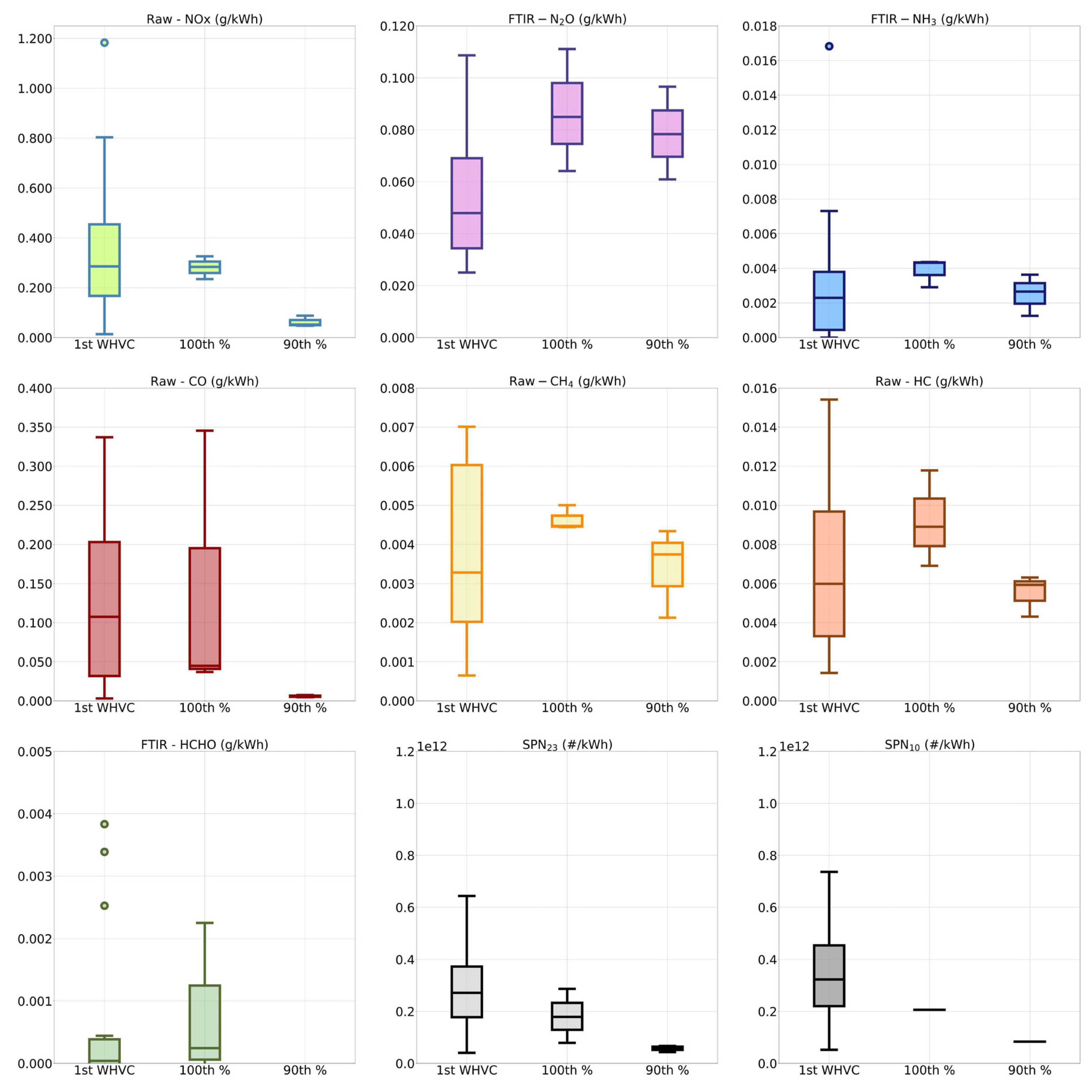
Figure 1 shows the aggregate results of the whole set of tests in the different conditions explored, calculated according to the procedure described in the “Evaluation Methodology” Section 2.5. Before proceeding with the discussion, it is important to point out that Figure 1 gives an overall picture of the emission performances of the vehicle without any ambition of being statistically representative, given the limited number of tests and the multiplicity of effects considered. It should be regarded as an indication of the emissions variability within loosely defined boundaries for operative conditions. It is also worth noting that the tests conducted did not cover all the possible conditions of use of this vehicle.

From the analysis of Figure 1, it is evident that the overall emissions of NH₃, CH₄, HC, HCHO are generally low, with very few cases in which 10 mg/kWh are exceeded. For this reason, in the following, the discussion focuses on the other pollutants, although all the data measured are available in Supplementary Materials for reference. It should be noted that, as already discussed in the “Evaluation Methodology” Section 2.5, no correction was performed for any of the instruments used in the campaign and, in this respect, all the data herein reported are to be considered “as measured”. It can be also noticed that SPN₂₃ and SPN₁₀ emissions are similar, with an additional fraction due to finer particles in the order of 15–25%; see also the detailed analysis in Figure S4 in Supplementary Materials. For this reason, in the following sections, the analysis focuses on NOx, N₂O, CO, and SPN₂₃, for which considerations will be less influenced by the experimental error, due to the higher quantities measured and due to the availability of SPN₂₃ for more tests (as detailed in the “VELA7 Heavy-Duty Test Cell” Section 2.2). In addition, the latter was less influenced by the experimental uncertainties due to possible interference from volatiles [14] as the system had an evaporation tube and not a catalytic stripper.

The median of NOx emissions in the short tests was in the order of 285 mg/kWh, with, however, a high variability (14–803 mg/kWh) in the emissions performances. A high emissions test of 1183 mg/kWh was also recorded in a low load urban test at −7 °C. This is discussed in more detail in the “Effect of Usage Patterns” Section 3.5 below. Generally speaking, long tests show comparable NOx emissions for the worst window (i.e., 100th cumulative percentile). The median for the 100th percentile of the MW cumulative distribution was 283 mg/kWh, with a much lower variability (235–326 mg/kWh). This was due to the fact that the long tests category included only three RWT cycles at different ambient temperature conditions (−7 °C up to 35 °C) with fixed 10% payload. Interestingly, the variability, which was induced only by temperature in this case, was minor. Moreover, the evaluation approach using MW allows granularity in the assessment of emissions. It isolates single high emitting events (included in the 100th and above the 90th percentiles) from a generally well-behaved average performance (ideally expressed by the 90th percentile). For this specific vehicle, the worst windows were always registered during cold start, when the emission control system was still cold an unable to effectively reduce NOx, as can be also graphically seen in Figure S5 in Supplementary Materials. Interestingly, for such cycles, very low NOx emissions could be still achieved for most of the cycle, with a 90th percentile of the windows distribution of 52 mg/kWh, with variability between 51 mg/kWh and 88 mg/kWh.

Qualitatively similar situations could be described for SPN₂₃ and SPN₁₀ with higher variability in shorter tests and decreasing emissions going from the 100th to the 90th cumulative percentiles of the MW distribution in long tests. A summary table reporting emissions results for all pollutants can be found in Table S3.

The median SPN₂₃ emissions for all performed tests was 2.71 × 10¹¹ #/kWh. SPN₂₃ varied between 4.03 × 10¹⁰ #/kWh and 6.61 × 10¹¹ #/kWh. On average, SPN₁₀ was 19% higher than SPN₂₃, this value varying from 15% to 29%. Note that SPN₁₀ was measured only for one out of three RWT cycles due to data logging issues. An overview of solid particle number emissions for each test can be found in Figure S4 in Supplementary Materials. Similar to NOx, at shorter cycles, higher variability of solid particle number emissions was observed, with decreased emissions going from 100th (>1 × 10¹¹ #/kWh) to the 90th (<9 × 10¹⁰ #/kWh) cumulative percentiles of the MW distribution in long tests at all temperature conditions (−7 °C, 23 °C, 35 °C).

N₂O and NH₃, despite the very low emissions of the latter, showed a different trend. Indeed, emissions factors were comparable in both short and long tests, without a clear distinction between the 100th and 90th percentiles. The median N₂O emissions for short tests were in the order of 42 mg/kWh, with variability between 10 mg/kWh and 109 mg/kWh. Long test emissions for the 100th and 90th cumulative percentiles were, respectively, 85 mg/kWh (variation 64–111 mg/kWh) and 78 mg/kWh (variation 61–97 mg/kWh). This indicates fairly continuous and low emissions, without significantly different events in the cycle such as cold start vs. stabilised hot emissions. This is in line with what was already reported in the literature [2,15] and consistent with possible pathways for N₂O production in Diesel emission control systems. Indeed, these are nowadays characterised by the requirement for very low NOx tailpipe emissions, requiring active DOCs, and an increase in the DEF injection rates together with the necessity of limiting any NH₃ slip at the tailpipe.

CO emissions were in the range of 0–350 mg/kWh in both short and long tests. The 90th cumulative percentile of the distribution of the windows was essentially close to zero. This indicated a very sharp and quickly decreasing distribution or, in other words, that for the tested system, most of the emissions were produced during cold start events.

HCHO emissions were very low and in the range of the experimental error of the instrument for all the tests considered and for this reason will be not discussed further. However, it is important to keep in mind that the measurement of aldehydes is generally complex [16]. Additional work will be needed to properly assess HCHO emissions from next generation vehicles.

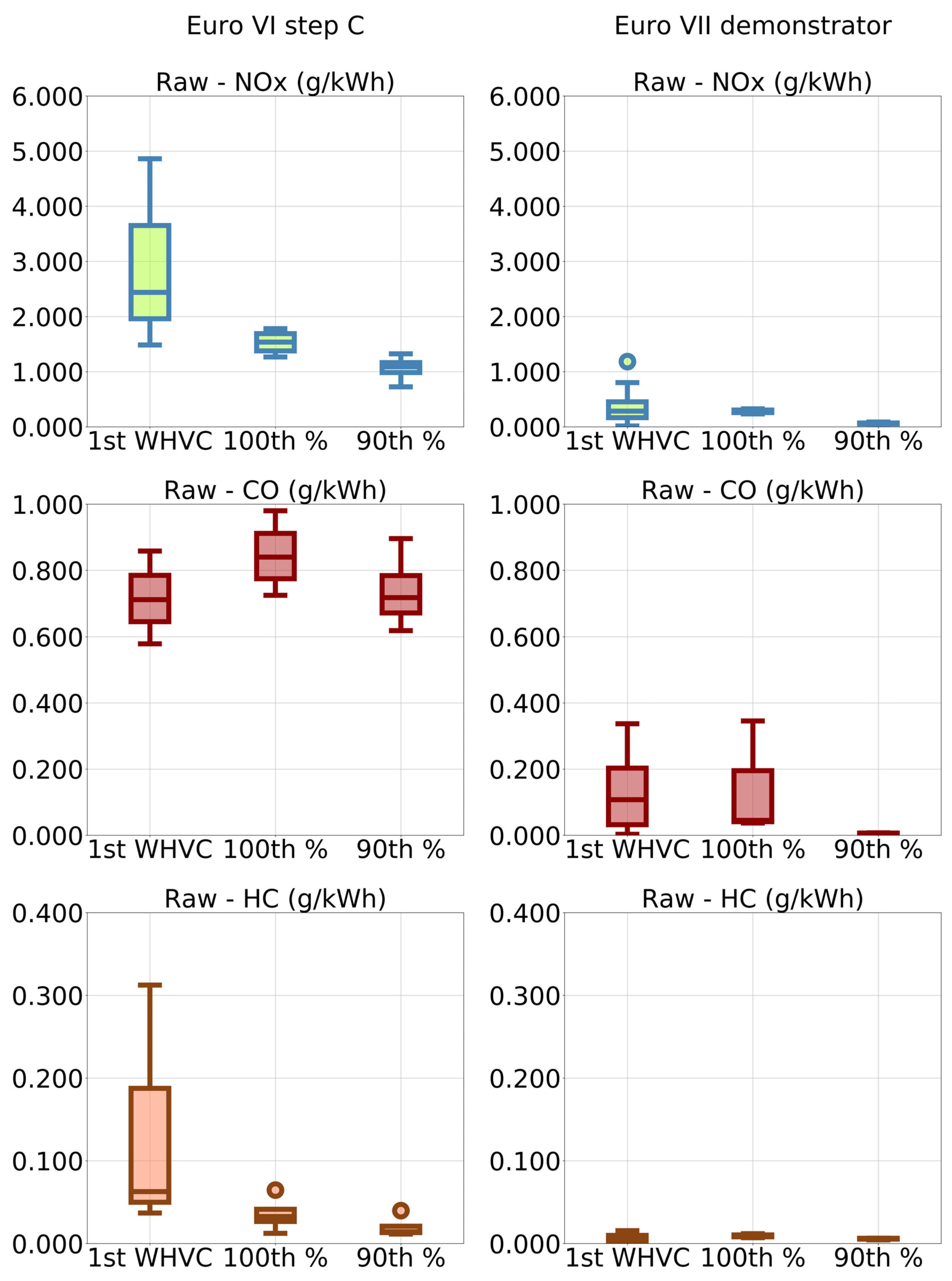
3.2. Comparison with Euro VI step C Vehicle

Figure 2 reports a comparison between a Euro VI step C vehicle and the vehicle object of this study. Note that for each pollutant, right panels include the same data already discussed in the previous section and are herein reported only for ease of comparison.

Although the Euro VI step C vehicle is not a “new” vehicle, and similar data could be found in the literature [2], the dataset herein reported was processed according to the same new method firstly introduced in this work and described in the “Evaluation Methodology” Section 2.5. Nevertheless, the test cycles performed in the two data set were not the same, even if they both comprised examples of simulated road driving in representative conditions. Additional information on the different routes and road gradients can be found in the “Vehicle and Tests” Section in Supplementary Materials.

Although mainly qualitative due to the limitations just described, this comparison shows an evident improvement in emission performances for all the pollutants considered, in line with what was also reported in [2] and in accordance to the evolution of air pollution regulations in Europe.

In particular, NOx emissions were reduced by approximately 9, 5, and 21 times for the short tests and the 100th and 90th cumulative percentiles of long tests, respectively. The variability was also drastically reduced, suggesting an increased robustness to varying operative conditions, especially considering that none of the Euro VI step C tests were carried out at sub-zero temperatures.

Similar reductions were seen in the case of HC emissions, with a decrease of the emissions of 12, 3, and 2 times in the same three cases.

Even more consistent improvements were achieved in the case of CO, with reduction of approximately 6, 19, and more than 2 orders of magnitude for short tests and the 100th and 90th cumulative percentiles of longer tests, respectively. These figures are in line with what was reported in literature, although it must be noted that the comparison was not done in perfectly comparable conditions, as already discussed [2,17,18,19].

3.3. Effects of Temperature

Figure 3 shows the effects of test temperature on the emissions of selected pollutants during cold RWT conducted at 10% simulated payload with a conditioned emission control system.

First of all, as expected, colder temperatures had a detrimental effect on the emissions of NOx. Total emissions increased from 9 to 11 g by changing ambient temperature from 35 °C to −7 °C, especially due to a more pronounced and extended cold start, as can be seen from instantaneous emissions profiles. This was mostly related to the increased difficulty in heating up quickly the SCR units and to reach the target temperature for DEF injection in colder conditions. In this respect, is also important to note that the test was started immediately after having switched on the engine, with no warming up period.

The situation was qualitatively similar for CO, in which however the impact of low temperature was much more pronounced. Indeed, colder emissions at −7 °C were approximately one order of magnitude larger with respect to those in milder conditions (10.5 g at −7 °C vs. 1.5 g at 35 °C). Additionally, in this case, high cold start emissions were predominant and likely related to inactive catalysts due to low temperature. It is important to mention that, in this period, emissions were essentially uncontrolled and equal to engine out emissions.

Interestingly, the situation was different for N₂O in which the impact of temperature was much less pronounced (overall emissions were between 5.7 g and 6.9 g for the temperatures tested) and with a very different emissions trend. Cold start was no more predominant, with instead continuous emissions throughout the test. This was already evident from the distribution of the 100th and 90th cumulative percentiles reported in Figure 1, and it is an indication of the different formation pathways with respect to other N-containing compounds (e.g., NOx). A more detailed discussion related to N₂O is done in the following sections.

No clear temperature effect was observed for SPN₂₃. At −7 °C and at 35 °C, the cumulative SPN₂₃ emissions (#) were 24% and 15% higher than at 23 °C, respectively, with the differences originating from some spikes during the cold start. Specific SPN₂₃ emissions (#/kWh) are presented in the Supplementary Information (Figure S4) and are calculated according to the approach described in the “Evaluation Methodology” Section 2.5. It can be noticed that the worst windows (i.e., the 100th cumulative percentiles) at −7 °C and 35 °C were 107% and 28% higher, respectively, with respect to the 23 °C case. The 90th cumulative percentiles were comparable for the 23 °C and 35 °C cases (2% difference) and 37% lower when comparing −7 °C to 23 °C. SPN₁₀ data were available only for the test performed at 35 °C, and it was 20% higher than SPN₂₃.

3.4. Effect of Payload

Figure 4 shows the effect of payload on the emissions of selected pollutants during cold urban delivery cycles conducted at −7 °C with a conditioned emission control system.

First of all, for NOx emissions, lower payloads had detrimental effects on emissions; at 10% payload, overall emissions were 19 g, while at 50%, they were 12.3 g. By inspecting the emissions profiles, it can be assumed that this was again due to the increased difficulty in quickly heating up the catalytic system and in maintaining the temperature during low load operations at such low temperatures and with a lower vehicle load. Indeed, at 10% payload, the cold start emissions had lower peaks but a more pronounced duration in time, and, at the end of the cycle (approximately at 3200 s), additional NOx were released. As can be also seen in Figure S2 in Supplementary Materials, this occurred after a sequence of prolonged idling phases of 3 min. This assumption was confirmed by the temperature profiles of the emission control system in the two cases (see Figure S6 in Supplementary Materials) where it is evident that a lower temperature was registered for the 10% case.

The situation was qualitatively reversed for CO. In this case, emissions were better controlled at lower payloads (7.6 g vs. 9.4 g). From the emissions profiles, it seems that this was due to a single event during cold start, a second peak at 250 s approximately. It is unclear whether this was due to an additional load required to the engine or to a slight variability in test execution, despite the faster heat up of the emission control system and of the DOC in particular.

N₂O emissions were again not significantly affected by the change in payload (total emissions were within 0.5 g in the two cases). This suggests that the control strategy of the emission control system was not significantly different in the two cases, resulting in a similar situation from a catalytic point of view. This in line again with the fact that N₂O formation was mostly related to the occurrence of unselective catalytic reactions and was not significantly affected by the engine behaviour.

Finally, for SPN, the situation was in line with that already described for CO. Emissions were more pronounced in the case of higher payloads (1.2 × 10¹³ # vs. 5.3 × 10¹² #), possibly due to the higher engine demand. When comparing specific SPN₂₃ emissions (#/kWh) calculated according to the approach described in the “Evaluation Methodology” Section 2.5, it can be noticed that at higher load they were 75% more. This finding is in agreement with previous studies that observed increased particulate mass [20] and particle number emissions [21] for higher loads of a heavy-duty diesel truck and bus, respectively. SPN₁₀ emissions were 25% higher than SPN₂₃ at 10% payload and 20% at 55% payload.

3.5. Effect of Usage Patterns

Figure 5 shows the effect of the utilisation pattern on the emissions of selected pollutants, using 10% payload, at an ambient temperature of −7 °C, with conditioned emission control system, and in cold starting conditions. Details on the three cycles considered here are reported in Figure S2 in Supplementary Materials and are summarised in the following for convenience.

The JRC cycle is characterised by a very low load, with maximum speed hardly exceeding 40 km/h and multiple stops of different duration up to 3 min. This was used to simulate the behaviour of an urban bus moving in a city and thus not representative of a N3 vehicle’s normal use, although in principle the same engine could be mounted also on a bus. The urban cycle is also a low load cycle with, however, higher maximum speed of 50 km/h, longer driving intervals, and fewer and shorter stops. This was used to simulate a delivery truck in a city environment. The RWT is a test that comprises urban, rural, and motorway sections, with maximum speed exceeding 80 km/h, varying road gradients, and few stops. This was used to simulate the real-world usage of a long haul truck, which is more similar to the design operation of the vehicle under test. Notice that urban and RWT cycle emissions are those already described in previous sections and are herein reported just for comparison purposes and not discussed again.

As expected, the JRC cycle was the most demanding in terms of NOx emissions due to the extremely low temperature and load. By the inspection of OBD readings and temperature profiles, it has indeed been confirmed that the DEF dosage unit never worked throughout the whole test (see Figure S7 in SI). This resulted in very high tailpipe emissions in line with those registered at engine out, reaching almost 35 g in total despite the short duration.

It is again interesting to notice how the situation for CO was qualitatively opposite with respect to NOx. Indeed, cycles with more demanding cold starts in terms of engine requirements resulted in higher emissions, while the JRC cycle, due to its very low load, resulted in only 6 g of total emissions. This was also in line with the effect of payload previously discussed.

N₂O emissions were essentially independent from the usage pattern, with differences in total emissions only related to the different test length. While a detailed discussion on the different chemistries leading to N₂O production is beyond the scope of this work, it is important to recall that nitrous oxide can be formed due to (i) unselective reaction between NH₃ and NO₂ on zeolite catalysts leading to formation and decomposition of nitrates [22]; and (ii) unselective NH₃ oxidation on ASC [23]; and (iii) as a by-product of NOx reduction by HC on DOC [24]. Importantly, all the above-mentioned mechanisms have distinct and hardly overlapping temperatures windows [24] requiring a complex and global optimisation of the whole emission control system. The theoretical absence of NH₃ in the system during the JRC cycle, due to the low emission control system temperature preventing DEF injection and to the preconditioning procedure consuming stored NH₃ and carried out the day before starting the test, suggests that the main production mechanism of N₂O in this vehicle was the one related to unselective NOx reduction by HC on the DOC. It is also worth mentioning that the temperature window for such a mechanism is consistent with what is indicated in [24] and measured for the system under test (see Figure S7 in Supplementary Materials). In any case, this behaviour will require additional investigation and it is an interesting point to keep in mind for system optimisation. In addition, this suggests that a complex interplay might exist between NOx, N₂O, and CO/HC emissions at least for the emission control system configuration studied.

SPN₂₃ emissions trends were different for the three cycles. While at the RWT and the urban cycle, cold start emissions dominated the total emitted particles (>60% during the first 500 s), this was not the case for the JRC cycle where SPN₂₃ emissions continued to increase during all its duration. The rationale was that during the JRC cycle, a stop and go cycle, SPN was emitted at each acceleration, and, thus, the cumulative SPN emissions continued to increase.

3.6. Idling

Figure 6 shows the emissions of selected pollutants during an idling test at an ambient temperature of 18 °C without preconditioning the emission control system, and in cold start conditions.

First of all, it is important to notice that the NOx concentration profile exhibited a significant delay of more than 800 s. After that, a large peak of approximately 90 ppm was released. This, as can be also noticed in Figure S8 in Supplementary Materials, incidentally coincided with the breakthrough of H₂O. Indeed, the exothermic stabilisation of H₂O immediately preceding its slip-on zeolite catalysts is well known to cause such an effect [25]; due to the rapid increase in temperature, desorption of NOx, or decomposition of nitrates can occur. Afterwards, NOx emissions were expected to progressively decrease to levels comparable with engine out steady state emissions. Unfortunately, the test was too short to see such an effect. It is also important to recall that before the test, the catalyst was not preconditioned (and thus adsorbed NH₃ should be available) and that the test was started hot, meaning that the emission control system was not completely cold.

The CO profile shows an interesting trend with a delay of approximately 300 s followed by a peak of more than 250 ppm and a subsequent drop in emissions.

N₂O emissions showed a peak of 20 ppm right at the very beginning of the test with very low values everywhere else. This initial peak was expected to be related to a continuous N₂O accumulation in the emission control system during the cool down until the temperature was sufficiently high to promote catalytic reactions, even with engine off. As soon as the engine was re-ignited, the N₂O accumulated was purged by the exhaust gases flowing through the system, resulting in a peak at test start. The accumulation in the sampling lines was, however, negligible. Indeed, by simply disconnecting them and leaving the instrument sampling, the measured concentration dropped to zero immediately.

PN emissions after the engine ignition and the first SPN₂₃ peak dropped and then increased and stabilised throughout the test in the order of 2.5 × 10⁹ #/s. This rate corresponded to a tailpipe concentration of 4.5 × 10⁴ #/cm³. The SPN₁₀ was ~15% higher than SPN₂₃, and thus the sub-23 nm particle fraction was very low.

3.7. Effect of Initial Status of the Emission Control System

Figure 7 shows the impact of the conditioning procedure described in the “Vehicle and Tests” Section 2.1. This consisted of driving the vehicle for approximately 30 min at high speed (70 km/h) with DEF dosing disabled. This promoted a passive regeneration of the DPF, avoided any clogging of the exhaust lines, consuming at the same time the NH₃ stored on the two SCR units. This also allowed the system to have similar starting conditions for the catalysts.

First, it should be noticed that, as expected, the effect on NOx emissions was significant. Indeed, a side effect of the conditioning procedure, due to the high-speed driving with deactivated DEF injection, was to consume all the NH₃ stored on the catalysts. This had the net result of strongly reducing SCR performance during cold start operations due to the absence of reactivity at low temperatures and the drastic reduction also of the possibility of storing NOx as nitrates on the catalyst. This was clearly evident inspecting the cumulative emission curves with a total NOx emission of 4.5 g vs. 19 g approximately in the two cases. Moreover, due to the average low load of the test, the temperature of the emission control system was generally low, making DEF injection problematic. This was evident in the last part of the test, where, after prolonged idling, additional NOx peaks were released in the case of a preconditioned vehicle. This was an indication also of the importance of a proper optimisation of the emission control system control and injection strategy.

The effect on CO was much less pronounced and inside the variability of the tests. From the emissions profiles, it seems that this was due to a single event during cold start, the second peak at 250 s approximately. It is unclear whether this was due an additional load required to the engine due to a slight variability in test execution.

The effect on N₂O was once again negligible. This was interesting and in line with what was discussed in the “Effect of Usage Patterns”. It seems that for this vehicle, the predominant mechanism for N₂O production was related to unselective reactivity on the DOC and not to routes involving the presence of NH₃. Indeed, overall emissions in the two cases matched quite well throughout the test, with an overall amount close to 2.5 g.

No effect of the conditioning was observed for SPN₂₃ and SPN₁₀ emissions. The conditioning cycle should have resulted in a passive regeneration of the DPF and thus a lower efficiency due to the low DPF fill state. There were no OBD data available to confirm whether the filter regenerated. Results indicated that either no regeneration occurred, or the regeneration was such that the DPF fill state was still high enough for the tests performed after it.

3.8. CO₂ Emissions with Contributions from Unregulated Pollutants

Figure 8 shows the average CO₂ emissions of the vehicle in both short and long tests, considering also the contributions of pollutants that, in addition to a negative impact on air quality [26], also promote global warming, namely N₂O and CH₄. However, in this specific case, the CH₄ contribution was negligible due to very low emissions, as discussed. From the Figure 8 it is first of all evident that the N₂O contribution to the CO₂ equivalent emissions, considering a global warming potential (GWP) for N₂O of 298 [27], was relatively small. The increase in CO₂ equivalent emissions due to N₂O was in fact in the order of 2.1–2.7% for both categories of tests considered.

To complement the analysis, it should be also noticed that CO₂ emissions were lower in the short tests if compared to both 100th and 90th cumulative percentiles of the distribution of windows obtained from long tests. This was mostly due to the fact that short tests comprised a significant number of WHVCs (8 tests), in which, due to the presence of sections of efficient driving on the highway, the CO₂ emissions were lower (728 g/kWh). In addition, a JRC city drive with long idling periods with low load (762 g/kWh) was also included. The set was completed by only four urban driving cycles for which the vehicle under testing, a long haul N3 truck, was clearly less optimised with average CO₂ emissions of 948 g/kWh. Indeed, in long tests, the worst windows were always related to urban driving patterns, with CO₂ emission figures for the 100th percentile (949 g/kWh) well in line with those registered in the shorter urban driving cycles.

3.9. Impact of Active Regeneration Events for Relevant Compound

Figure 9 shows the emission profiles during the active regeneration of the DPF filter for selected pollutants. Two things should be noticed: (i) during this test, raw gaseous compound measurements were carried out only with a HORIBA MEXA-ONE-QL-NX measuring NOx, NH₃, and N₂O, while all the other tailpipe instruments were not measuring; (ii) the service regeneration procedure was triggered. This is important, since this is the one defined for the EU VI step C production system and has not been specifically adapted for the EU VII demonstrator. In addition, such a procedure is usually only used if the vehicle cannot clean the DPF during normal driving, being therefore a function for hardware protection not to be misunderstood with an active regeneration on the road. The whole test was performed in idling conditions, at an engine speed of 500 rpm.

The first important thing was that the regeneration, starting around second 1500, was not complete even after 40 min, considering that approximately 20 min passed before triggering the regeneration. After the initial increase, the emissions stabilised to about 700 ppm for NOx and 1 × 10¹⁰ #/s for SPN₂₃. Overall, approximately 148 g of NOx were emitted during the test, and 2.45× 10¹³ # of SPN₂₃, N₂O, and NH₃ emissions were lower, with rates of 4.1 g and 0.4 g, respectively. For consistency with the rest of the work, SPN₂₃ are reported in the figure, noticing however that SPN₁₀ was ~10% higher than the SPN₂₃ during the active regeneration.

Before the regeneration, the emission control system was not conditioned, and the Brenner cycle and the idling test were performed since the last preconditioning procedure. This might be relevant in terms of NH₃ and N₂O emissions, since, as already discussed during the idling test (which was performed just before the regeneration one), a long induction period before NOx breakthrough was recorded. This suggests a progressive consumption of the NH₃ stored on the catalyst. Indeed, this might imply that NH₃ and N₂O can be proportionally higher if active regeneration was carried out with a different starting catalyst history, as also shown in the literature [4]. Similarly, for PN, the stored material in the DPF has an influence on the emitted particles [28]. Nevertheless, the total emitted particles of 2.45 × 10¹³ # of SPN₂₃ were within the range reported for solid particle emissions during “parked” regeneration (1.5–5.1 × 10¹³ particles) [29].

3.10. Assessment of Instruments for On-Road Measurement of N₂O and NH₃

Figure 10 shows the results of the correlations between the N₂O measured concentrations by two different portable (OBS-ONE-XL and LAS-N₂O) and laboratory (AVL SESAM and HORIBA MEXA-ONE-QL-NX) instruments. The whole set of time-aligned 1 Hz measurement was used for this inter-comparison except for two experiments (a WHVC hot, 23 °C, 55% payload and the RWT cold, −7 °C, 10% payload) in which the instruments showed a malfunction.

The upper panels show that the OBS-ONE-XL and both laboratory grade instruments excellently correlated, with an R² > 0.96 in both cases and a very good linearity, with angular coefficient equal to 1 ± 0.05 and intercept < 0.2. These results were well in line with those obtained for a CNG M1 bus and discussed in [11].

The bottom panels show that also for the AIP LAS-N₂O, measurements excellently correlated with both laboratory grade instruments, with an R² > 0.94 in both cases and a very good linearity, with angular coefficient equal to 1 ± 0.07 and intercept < 0.1.

NH₃ emissions were generally low for this vehicle, and this was confirmed by all the instruments used in the campaign. Additional details can be found in Figure S9 in Supplementary Materials.

3.11. Assessment of Onboard Measuring Systems

Figure 11 reports a comparison between the NOx emissions obtained using the on-board sensors of the vehicle and those determined with laboratory grade instrumentation. In both cases, the flow rate used was the one calculated by subtracting the CVS total flow rate and the measured dilution air. In general, it can be seen that sensors slightly overestimate emissions, with a deviation in the order of 15% on the median for the short tests and up to 50% for the 100th cumulative percentile in long tests. The error further increased for the 90th percentile, very likely due to the very low concentrations of NOx measured after the SCR became fully operational, as can be seen in Figure S10 in Supplementary Materials. This promising result showed the potential utilisation of on-board sensors to monitor emissions performance on vehicles on the market; such sensors easily discriminate potentially high emitting behaviours or tampered vehicles, provided that are properly implemented.

4. Conclusions

This work summarised the emissions performance of an advanced demonstrator N3 vehicle with a specifically designed emission control system thermally aged to 500k km equivalent. The vehicle was tested in the laboratory in a large variety of conditions in terms of ambient temperature (from −7 °C to 35 °C), payloads (10–55%), and operative conditions ranging from urban delivery cycles to aggressive motorway driving, including idling and DPF regeneration. The demonstrator vehicle and emission control system generally controlled well the emissions, which were substantially lower than those reported for Euro VI vehicles. Still, a large variability in emissions was induced by the broad range of operative conditions, including during cold start. The scattering found due to the impact of the NOx storage capability of the catalyst system, water absorption, and release played a part in the amount of NOx emissions measured during the cold start. Furthermore, effects of temperature and payload also played a role.

The effect of emission control system conditioning was also explored, showing the importance of a robust control strategy and a properly operating SCR system to effectively reduce NOx emissions, also in challenging operative conditions such as cold start.

Among currently unregulated pollutants investigated, the emissions of N₂O were the most relevant for this specific vehicle. These seemed to be related to unselective reactions ongoing in particular on the DOC, but this hypothesis requires further investigation. The increase in CO₂ equivalent emissions due to N₂O was approximately 2.5% under the conditions explored. N₂O and NH₃ were also measured by two new generation portable instruments, which showed excellent correlation with laboratory grade reference instrumentation, supporting the possibility of effectively measuring such species during on-road testing. The increase of particle emissions due to the inclusion of SPN₁₀ were in the order of 20–25% depending on the testing conditions.

Finally, the performance of on-board sensors for the measurement of NOx was also studied. The assessment showed encouraging results, strengthening the idea that they may be suitable to detect high emitting or tampered vehicles, by monitoring these sensors when properly implemented.