1. Introduction
The energy demand in the residential sector represents 28% of the total final energy consumption in the EU (62% of the energy consumption of buildings) [
1]. The largest energy consumption is dedicated to heating (almost 64%), followed by domestic hot water production (DHW) (15%) [
1]. About 76% of this energy is based on fossil fuels. Heat pumps are highly efficient electrically powered devices that can be used to meet the demand for heating, cooling, and/or DHW production. In addition, they do not produce local emissions and can therefore contribute significantly to increase the energy efficiency of buildings. This, and the foreseeable increase in renewable energies in electricity generation in the EU, suggests a considerable increase in sales of heat pumps, which will ultimately help to reduce the carbon footprint of the building energy sector [
2].
The heating requirements in a building or in a space depend largely on the outdoor temperature.
Figure 1a shows the typical evolution of the heating power demand or heating load curve of a building or dwelling (
) as a function of the outdoor temperature (
Tj). The heating thermal load increases as the outdoor temperature decreases. The slope of this curve depends on several factors such as the level of insulation of the house, the glazed surface, the level of ventilation, etc. The design load (
) is the thermal heating load for the design temperature (
Tdesign). The temperature designated as
Tlim is the temperature above which heating is no longer required.
Figure 1a also shows a typical curve of the heat output supplied (
) by a heat pump with a single fixed speed compressor (on/off operation), as a function of the outdoor temperature. The curve represented in this figure could be a typical one of an air-source heat pump, highly dependent on the temperature of the external environment. In the case of a geothermal heat pump, the slope would be much lower or almost zero since it can be assumed that the ground temperature is practically constant and independent of the outdoor temperature.
In
Figure 1a, it can be seen that the curves
and
have only one point of intersection. The outdoor temperature corresponding to this point is called the bivalent temperature (
Tbiv). When
the heating demand cannot be supplied by the heat pump alone and a supplementary system is necessary (for example, an electric heater). On the other hand, when
, the power supplied by the heat pump is greater than the heating load, so the heat pump will necessarily have to switch into on/off operation to adjust its heating capacity to the heating demand. Finally,
Figure 1a also shows that there is an operation limit temperature (
TOL) below which the heat pump will not function and will not deliver any heating capacity.
Figure 1b shows the situation for a variable speed compressor that can change its rotational speed between the values
and
. Two heat pump curves are represented in the figure, one for the maximum compressor speed and another one for the minimum compressor speed. As before, the maximum speed curve intersects the heating demand curve at the bivalent temperature (
Tbiv). A second temperature (
Tbiv*) can be defined as the temperature for the point of intersection between the heating demand curve and the heat pump curve for the minimum compressor speed. When
, the power supplied by the heat pump (even with the compressor at the minimum rotational speed) is still greater than the heating load, so cycling (on/off) operation would be required to match the heating load. However, when
, the heat pump can modulate its capacity to satisfy the heating demand, by varying the compressor speed. Therefore, a heat pump that incorporates a variable speed compressor will probably provide higher seasonal energy efficiencies than a fixed-speed one by reducing the number of on/off cycles, as well as by providing higher COPs at part load.
In addition to the technological evolution from fixed speed to variable speed compressors, many current heat pumps have a weather compensation control that allows the unit to adjust the water flow temperature depending on the outdoor conditions. This is based on the idea that at part load, the supply temperature to the terminal units of the heating system can be lower than at design conditions. Then, for this type of unit, as the outdoor temperature increases and the heating load decreases, the heat pump supplies water at lower temperature. As a result, the condensing temperature decreases at part load leading to higher COP values.
The seasonal coefficient of performance (SCOP) of a heat pump describes its average performance during the heating and/or cooling season, considering the different energy demands and their variability over time. Many authors have chosen the SCOP as an adequate metric parameter for evaluating the effect of refrigerant drop-in studies [
3,
4], the effect of the type of compressor used (mono-compressor on/off, multi-compressor, or variable speed compressor) [
5,
6,
7], the effect of the selected bivalent temperature [
5,
8], the effect of different control strategies [
9], or for CO
2-emissions and economic analyses of different heating technologies [
10].
In Europe, Commission Regulation (EU) No. 831/2013 establishes the ecodesign requirements for space heaters, including heat pumps, which evaluation requires the calculation of their seasonal coefficient of performance (SCOP) [
11]. The part load testing conditions and the calculation methods to be applied in order to determine the seasonal coefficient of performance are described in EN 14825:2018 standard [
12].
This paper is focused on a brine-to-water heat pump for low-temperature applications. The main components of the unit are a variable-speed Scroll compressor, an electronic expansion valve, and brazed-plate heat exchangers for the indoor (water) and outdoor (brine) heat exchangers. The methodology to determine its seasonal coefficient of performance (SCOP) according to the European standard EN 14825 is explained and evaluated based on experimental results. In order to evaluate the impact of different technological and control options, we present and compare SCOP results operating the heat pump with the compressor at fixed speed (at full speed) and at variable speed, as well as considering that the heat pump has fixed or variable outlet temperature operation.
2. Heat Pump Description
Figure 2 shows a schematic representation of the heat pump considered in this work. It is a brine-to-water heat pump; the baseline refrigerant is R410A. Refrigerant R410A has a Global Warming Potential (GWP) of 1925 (AR5), so various lower-GWP alternatives have been proposed in recent years, such as R32, R452B, or R454B. Drop-in performance tests for some of these alternatives were previously evaluated by the authors for selected operating conditions [
13]. Future analyses, using the SCOP methodology presented in this paper, will allow a more adequate evaluation of alternative refrigerants.
The main components of the heat pump are a variable speed Scroll compressor, an electronic expansion valve, and plate heat exchangers for the condenser, evaporator, and desuperheater. The desuperheater may be used for domestic hot water production, though it was not used in this work.
The compressor’s drive has a cold plate heat exchanger in order to avoid high internal temperatures. Water is used for cooling the drive and for the condensation process. As shown in
Figure 2, of the total flow rate in the water loop (measured by the flowmeter
Vw), a small fraction is diverted to the drive heat exchanger (measured by the flowmeter
Vw,cd) and the remainder flows through the indoor heat exchanger (condenser). The two water flows are mixed at the outlet of the unit. In the evaporator, a propylene glycol-water mixture (
PGw) with a concentration of 24% by mass of propylene glycol is used as the heat exchange fluid.
The heat pump was equipped with appropriate instrumentation in order to measure its SCOP.
Figure 2 shows the location of some relevant sensors used in the experimental setup and
Table 1 summarizes their main characteristics. More details about the experimental setup and the instrumentation can be found in previous works [
13,
14].
3. Basis of SCOP Testing and Calculation
In order to evaluate the seasonal performance of the heat pump, the calculation process established in EN 14825:2018 was followed. This requires testing the heat pump unit at different part load conditions as well as the determination of its energy consumption at different non-active modes of operation, such as thermostat off mode, standby mode, off mode, and crankcase heater mode.
3.1. Declared Heat Output and COP
For any test condition, the declared heat output and
COP of the heat pump was determined in accordance with standards EN 14511-2:2018 [
15] and EN 14511-3:2018 [
16].
The electrical power input to the heat pump (
) includes the power input for driving the compressor (
), the powers required by the water and
PGw pumps (
and
) for the transport of both fluids through the heat pump unit, and any additional electrical power input (
) required by the heat pump (such as control and safety devices).
In this work, the water and
PGw pumps are not integral parts of the heat pump. The pump powers to be included in the effective power consumed by the heat pump are estimated using the following formulae, based on the hydraulic power and the pump efficiency values [
16].
In the previous equations, the hydraulic power is determined from the measured liquid flow rate and the measured heat pump-side static pressure difference:
For the pump efficiencies, the formula proposed by EN 14511:3:2018 for pumps that are not an integral part of the heat pump unit was used.
The heating capacity supplied to the water flow is determined from an energy balance between the water conditions at the inlet and outlet of the heat pump:
This capacity is corrected for the heat from the circulating pump, according to EN 14511-3:2018,
Finally, the declared coefficient of performance (
COPd) is calculated from the net heating power and the effective power input:
3.2. Part-Load COP
The seasonal coefficient of performance (SCOP) describes the heat pump average performance during the heating period. It can be used to evaluate how well a heat pump will behave for a particular heating demand curve.
The combination of the outside temperatures (
Tj) in a locality and the number of annual hours (
hj) in which these temperatures are recorded is known as the temperature period (
binj). The EN 14825 standard defines three reference climate conditions: average ‘A’, coldest ‘C’, and warmest ‘W’, for their corresponding three characteristic reference heating stations in the cities of Strasbourg, Helsinki, and Athens, respectively.
Figure 3 shows the number of hours in each bin for each of the three reference climate conditions.
To determine the SCOP of a heat pump in accordance with EN 14825, first the heating demand curve must be determined as a function of the outdoor temperature. The part load factor (
pl) is the ratio between the heating load at a specific temperature
Tj and the design heating load at the design temperature
Tdesign:
The EN 14825 standard assumes that the part load factor varies linearly with the outside temperature. Then, since the heating load is zero at the heating temperature limit (
Tlim), the demand curve can be determined once the design heating load (
) at the design temperature (
Tdesign) is established.
If the heat pump is a fixed capacity unit, it will need to perform cycling (on/off) operations to achieve the heating load. In the case of a unit with a variable speed compressor, the unit can modulate its capacity by continuously adjusting the compressor rotational speed within the limits of minimum () and maximum () speed of the compressor.
Let us designate as
the heating power supplied by the heat pump for the temperature interval (
Tj) and as
the heating load for the same temperature. If
the unit switches to on/off operation to adjust its heating capacity to the heating demand. The capacity ratio (
CR) is defined as:
In these cases, a degradation coefficient (
Cd) must be determined by performing a specific test (or a value of 0.9 might be assumed according to the standard) to determine the energy consumption of the heat pump when the compressor is off. It should be noticed that even when the compressor is off, the heat pump energy consumption is not zero because of the energy used by the heat pump auxiliary devices.
The part load
COP for each temperature bin is calculated as:
where
COPd is the declared
COP measured by testing the unit at the required part-load capacity or estimated by interpolation between COPs measured below and above the required capacity. If the heating load is lower than the minimum capacity of the heat pump, the
COPd at the minimum capacity is used.
If , then it is considered that the heat pump works at full capacity (CR = 1) and the COP corresponding to the temperature period (binj) is the declared COP measured or calculated by linear interpolation between the nearest heating load conditions, i.e., .
3.3. Caculation of SCOP
The SCOP can be calculated from the heating load demand and the results of the heating capacity and COP of the heat pump for each temperature period.
The annual heating demand for any temperature period (
binj) is obtained from the heat load and the number of hours (
hj) for the temperature period:
The total annual heating demand is calculated as:
If for a given temperature interval (
Tj) the capacity is lower than the heating load, i.e.,
, it is assumed that the heat pump capacity is supplemented by an electric backup heater.
Therefore, if for each temperature period (
binj) the heat pump performance is given by
, the annual energy consumed by the heat pump and by any supplementary heaters is calculated as follows:
The seasonal coefficient of performance in active mode (
SCOPon) is defined as the annual heating demand (
Qb) divided by the annual electrical consumption of the heat pump during active mode (
Eon).
The total seasonal coefficient of performance (SCOP) considers the energy consumption in active mode, as well as the energy consumption in operating modes other than active. The energy consumption of the unit during thermostat off, standby, off mode, and crankcase heating modes of operation is estimated as a function of the number of hours for each mode of operation (values given by the EN 14825 standard) and the power consumption of the heat pump unit in each mode (which are measured by specific additional tests).
3.4. Relation with Ecodesign Requirements
Electrical driven space heaters, such as heat pumps or electric boilers, account for a large share of the total energy demand in the EU. In order to reduce the energy consumption of this (and other) equipment, the EU introduced minimum energy efficiency and energy labelling requirements for space heating devices. The Commission Regulation (EU) Nº 813/2013 establishes ecodesign requirements for placing on the market space heater and combination heaters with a rated heat output lower than or equal to 400 kW [
11]. The requirements for the space heating efficiency are based on the value of the seasonal space heating efficiency (
) under average climate conditions. This efficiency is calculated as:
where
CC is a conversion coefficient equal to 2.5 that reflects the estimated 40% average EU generation efficiency and
F(1) and
F(2) are correction factors. For brine-to-water heat pumps, the corrections are
F(1) = 3% and
F(2) = 5% and account for the contributions of temperature controls and pumps. Therefore, the space heating efficiency of a heat pump depends basically on its SCOP value.
The Regulation (EU) Nº 811/2013 introduced an energy labelling scale from A
++ to G for space heaters [
17]. The energy efficiency class of a heat pump for space heating is based on the value of its seasonal space heating efficiency (
).
From 26 September 2017, the minimum requirements for seasonal space heating energy efficiency in the case of heat pumps for low-temperature applications is 125% which corresponds to an energy efficiency class A+ or better.
4. Results and Discussion
A set of experimental tests were performed in order to determine the SCOP of the heat pump following the methodology described in the EN 14825 standard, for brine-to-water heat pumps for low temperature applications. In this paper, the SCOP is only evaluated under the average climate conditions, which are the mandatory ones in European energy labelling regulations [
11,
17].
Table 2 shows the part load test conditions for the average ‘A’ climate conditions. The reference design temperature for heating is
and the heating limit temperature is
. The heat pump test bench is equipped with variable flow pumps, so for all conditions a temperature variation of 5 K was maintained in the water circuit of the indoor heat exchanger (HEx) and 3 K in the
PGw circuit of the outdoor heat exchanger. In all cases, the tests were performed controlling a degree of superheat at the evaporator outlet of 7 K.
The rated heat output of the heat pump is the declared heat output at the design temperature with the compressor running at maximum speed (i.e., ). A value of was obtained testing the unit in accordance to EN 14511-2:2018 and EN 14511-3:2018.
In this work, the bivalent temperature (
Tbiv) was selected equal to the design temperature (
Tdesign). The design heating load is equal to the rated heat output of the heat pump (i.e.,
) and, consequently, the test conditions E and F in
Table 2 are the same. Once the design load was established, the part-load tests A to D were performed for the following four scenarios:
The compressor operates at fixed speed (maximum speed). Even though the heat pump has a variable speed compressor, it is tested and its SCOP is evaluated as if it were a fixed speed compressor. Additionally, tests are performed for fixed outlet temperatures in the indoor heat exchanger. This case is denoted as Cf&Tf (Compressor fixed and Temperature fixed).
Same as before but with variable outlet temperature. We denote this case as Cf&Tv.
Cv&Tf case which comprises a heat pump unit with variable speed compressor and fixed outlet temperature. The compressor speed is adjusted to achieve the part heating load required at each part-load test condition.
Heat pump with a variable speed compressor and variable outlet temperature, designated as Cv&Tv.
Figure 4 shows the heating load curve, and the heat output curve and the
COPbin of the heat pump as a function of the outdoor temperature. Results are shown for the heat pump operating with fixed outlet temperature and with the compressor running at fixed and variable speed (Cf&Tf and Cv&Tf, respectively). In the figure, the points with legends A to F are experimental values at part load conditions. Heat capacities and
COP values for other temperature intervals were obtained by interpolation or based on the limiting test conditions (at minimum or maximum compressor speed).
Figure 4a shows the results obtained with the heat pump assuming that the compressor operates at fixed speed. For each part load test condition, the declared heat capacity (
) and the declared coefficient of performance (
) are constant since the fluid temperatures in the indoor and outdoor heat exchangers do not change and the compressor operates at fixed speed. For outdoor temperatures below −10 °C (point E) the heat pump cannot meet the heating load, but for temperatures above −10 °C the heat pump needs to perform on/off cycles in order to adjust its heat output to the heating load. The bin-specific coefficient of performance (
) is derived from the declared
COP and corrected by the degradation coefficient (
Cd) that accounts for the heat pump energy consumption when the compressor is off (see Equation (14)). When the outdoor temperature increases, so does the difference between the heating capacity and the heating load, resulting in lower values of the capacity ratio (
CR) and a higher weight of the degradation coefficient on the
COPbin. As a result, the
decreases slightly with increasing values of the outdoor temperature, as confirmed in
Figure 4a.
Figure 4b shows the results when the compressor operates at variable speed. For outdoor temperatures below −10 °C (point E) the heat pump cannot meet the heating load, whereas for temperatures above 7 °C (point C) the power supplied by the heat pump is greater than the heating load, so on/off cycling will be required. Between the outdoor temperatures corresponding to points E and C, the compressor adjusts its rotational speed to adapt its power to the required heating load. With regards to the bin-specific coefficient of performance, it can be seen that for outdoor temperatures below −10 °C (point E) the value of
is constant; this is explained by the fact that for
the heat pump operating conditions and compressor speed do not change. As the outdoor temperature increases from −10 °C (point E) to +12 °C (point D), the compressor rotational speed decreases from its maximum (7000 rpm) to its minimum (1800 rpm) value. The
COPd first increases with a reduction of the rotational speed when changing from part-load conditions E to B. However, further reductions of the heating load and consequently of the compressor speed produces a decrease of the
COPd value. For part-load factors below that of point C (35%), the
continues to decrease due to the decrease of
COPd and the greater impact of the degradation coefficient (
Cd) because of on/off operation, as stated in Equation (14).
The results for a heat pump with variable outlet temperature with fixed and variable speed compressor operation are shown in
Figure 5. Now, when the outdoor temperature increases, the heat pump reduces the supply water temperature as indicated in
Table 2. Consequently, the heat pump operates at lower condensation temperatures and with higher
COP values.
For the fixed compressor speed option (Cf&Tv), as the outdoor temperature increases, the
COP of the heat pump increases substantially whereas the heat capacity remains nearly constant. For the variable speed case, a comparison of
Figure 4b and
Figure 5b show that the variable outlet temperature option (Cv&Tv) is similar to the fixed temperature one (Cv&Tf) in terms of heat output, but it is superior in terms of
COP.
Once the heating load and the heat capacity and COPbin curves of the heat pump are determined, the heat demand and the energy consumed by the heat pump for each bin can be evaluated.
Figure 6 shows the bin hours at each outdoor temperature for the average climate conditions as well as the heat demand and the energy consumption of the heat pump. The results are shown for the four heat pump options considered: Cf&Tf, Cv&Tf, Cf&Tv, and Cv&Tv. For all cases, the heat demand is the same; however, there are differences in the energy consumed by the heat pump. The design temperature under the average climate conditions is −10 °C. As shown in
Figure 6, this is the minimum expected temperature, so the number of annual hours for temperature values below −10 °C is zero. As a result, for the situation considered in this work, the heat pump can always satisfy the heating demand and a backup heater is not required. As expected, the energy consumed by the heat pump is reduced when the use of variable speed compressors or variable outlet temperature operation are considered.
By adding all heat () and energy input () values for each outdoor temperature (Tj), the annual heat demand, the annual energy consumption, and the active mode seasonal coefficient of performance (SCOPon) can be obtained, using Equations (15)–(20).
In order to obtain the total seasonal coefficient of performance (SCOP), the energy consumption of the unit during compressor off mode, thermostat off mode, standby mode, off mode, and crankcase heater mode were also determined as per EN 14825:2018. The compressor-off mode is required for the calculation of the degradation factor (Cd) when the heat pump heating capacity is greater than the heating load. The results from these tests are collected in
Table 3. As shown, when rounded to the nearest integer, the power consumption values measured for each mode of operation were the same for the four heat pump options. It should be clarified that the standard only considers losses associated with the heat pump unit. In a real installation, other energy losses will appear which will depend on various factors related to the heating installation, such as the type of terminal units or the use of buffer tanks for reducing the frequency of on/off cycling.
Once the active and non-active energy consumptions are determined, the SCOP and the seasonal space heating efficiency (
) can be obtained.
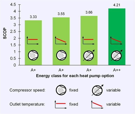
Table 4 shows the SCOP and
calculated values for the four heat pump options, as well as the corresponding energy efficiency class according to Regulation (EU) Nº 811/2013. As shown in the table below, technical evolutions such as variable speed compressors or weather compensation controls that act on the flow temperature can contribute to important energy efficiency improvements of heat pump units.


