Preemptive Priority Markovian Queue Subject to Server Breakdown with Imperfect Coverage and Working Vacation Interruption

Abstract

This work considers a preemptive priority queueing system with vacation, where the single server may break down with imperfect coverage. Various combinations of server vacation priority queueing models have been studied by many scholars. A common assumption in these models is that the server will only resume its normal service rate after the vacation is over. However, such speculation is more limited in real-world situations. Hence, in this study, the vacation will be interrupted if a customer waits for service in the system at the moment of completion of service during vacation. The stationary probability distribution is derived by using the probability generating function approach. We also develop varieties of performance measures and provide a simple numerical example to illustrate these measures. Optimization analysis is finally carried out, including cost optimization and tri-object optimization.

1. Introduction

Motivated by computer systems, manufacturing and production systems, communication systems, service systems, and many other real-world systems, many authors have studied queueing models with server vacations. For an extensive review of this topic, one can refer to Tian & Zhang [1] and Ke et al. [2], who discussed in detail the related research on different vacation policies. Based on the classical vacation, the working vacation policy was introduced by Servi and Finn [3]. In such a policy, during the vacation period, the server works at a relatively slow rate instead of stopping completely. Tian et al. [4] reviewed the research on working vacation queueing systems. Recently, the survey on the works of queues with working vacation has been reported by [5,6,7,8,9,10,11,12,13].

Vacation interruption is another important concept for efficient server utilization. Li and Tian [14] introduced this concept into a single server queueing system with vacation. Lee [15] introduced the concept of vacation interruption into a Markovian queueing system under a single working vacation policy to investigate equilibrium analysis. Bouchentouf et al. [16] established a cost optimization analysis for a finite-buffer queueing system with impatience behavior. They assumed that the single server has two types of vacation and the vacation can be interrupted under Bernoulli scheduling. Shekhar et al. [17] studied a randomized arrival control policy for potential customers in the finite-capacity vacation queueing system with vacation interruption. Vijayashree and Ambika [18] considered a queueing system with impatient customers, where the single server has two types of vacation. The exact analytical expression for the time-dependent probabilities is obtained.

Unreliable servers are also a realistic feature observed in many practical applications. The server breakdown situation may influence the queueing system output, thereby reducing the system’s efficiency. To overcome this, the queueing system must be equipped with a repair facility to reduce service delays because of server failures. Unreliable queueing systems have been studied by many researchers [19,20,21,22], and one of the basic assumptions is that once a server fails, it is repaired immediately. In addition, the notion of coverage and its impact on unreliable queuing systems has been introduced by several authors.

The assumption that customers are served according to their order of arrival is common in queueing systems. However, we may need to control queueing systems through a priority mechanism to provide different quality services to different types of customers. For this reason, various priority disciplines are used in many computers, manufacturing, telecommunication, and operating systems. The server provides service to high-priority customers based on the preemptive and non-preemptive disciplines. In preemptive disciplines, high-priority customers are allowed to interrupt the service of low-priority customers. In the non-preemptive case, the service of already started customers with low priority will not be interrupted, even if a high-priority customer arrives during the service period. Brandwajn and Begin [23] proposed an approximate solution for the multi-server preemptive resume priority queueing system in which the interarrival and service times follow arbitrary distributions. Wang et al. [24] dealt with the customer’s equilibrium strategies in a queueing system with a pay-for-priority option. Kim [25] developed a delay cycle analysis to analyze priority queues under non-preemptive and preemptive resume priority disciplines. Kim et al. [26] investigated a multi-server queue with multiple vacations under a non-preemptive priority schedule. They also investigated the customer’s equilibrium strategy and the social cost minimization problem. Ajewole et al. [27] discussed a preemptive resume priority queueing system, where the service time obeys the Erlang distribution. The Laplace transform representation for the generating function of the duration of a busy period for the higher priority class including the associated moments is obtained. The performance measures for the system size and sojourn time for the lower priority queue in equilibrium are also determined. To the best of our knowledge, there is no paper analyzing the multi-objective optimization issue of the preemptive priority Markovian queue, which is affected by the server breakdown with imperfect coverage, and working vacation interruption.

We organize the rest of the paper below. Section 2 describes the model and assumptions. Section 3 analyzes the stationary probability distribution. A brief overview of some performance measures is derived from the steady state distributions in Section 4. Section 5 illustrates the results of the numerical study and analyzes optimization problems, including cost optimization and tri-object optimization.

2. System Description

Consider a single server preemptive priority queueing system accepting class-1 customers and class-2 customers. Class-i customers join the system according to the Poisson process with rate λ_i for i = 1,2. Class-1 customers have preemptive priority head of the line priority over class-2 customers in the service time of the busy server. If the server is available on the arrival of a customer, the arriving customer gets its service immediately. The newly arriving class-1 customer will wait in the system if the server is occupied by a class-1 customer upon arrival. While the server is serving a class-2 customer, the arriving class-1 customer will interrupt the service of the class-2 customer and receives service immediately. Suppose that the class-2 customer preempted by a class-1 customer will be resumed again as there are no class-1 customers in the system.

In the normal busy period, the service times of class-i customers obey exponential distribution with rate μ_i, i = 1,2. Once the system empties, the server takes a working vacation. The duration of the server vacation obeys an exponential distribution with rate η. During a working vacation period, if any customers arrive, the server could continue to provide service according to an exponential distribution with a low rate θ_i (<μ_i), i = 1,2. If there are any class-1 (or class-2) customers in the system at the moment the lower-speed service is completed during the working vacation period, the server will interrupt the vacation and switch the service rate back to the normal busy period. Otherwise, the server continues the vacation.

The server is subject to breakdowns during the normal busy period and working vacation period. The breakdown is generated by an exponential distribution with the state-dependent rate α_k (k = b, v), where k denotes the state of the server. The probability of detecting and locating a failed server immediately is assumed to be q. If the failed server is successfully detected, it is sent to a repair facility for repair. Repair time is exponentially distributed with the state-dependent mean 1/β_k (k = b, v), where k denotes the state of the server. Otherwise, the repair facility will enter an unsafe state. The repair facility will issue a reboot operation to locate the undetected failed server to clear the unsafe state. The reboot delay time is exponentially distributed with mean 1/γ. Assume that the time of the reboot period can be ignored. Hence, during that time, the arrival of a customer is neglected and the server stops his work.

The arrival load is defined as ρ = ρ₁ + ρ₂ = (λ₁⁄μ₁) + (λ₂⁄μ₂). Suppose that ρ(1 + (α_b⁄β_b)) + σ(1 + (α_v⁄β_v)) < 1 for the stability of the system, where σ = (λ₁⁄θ₁) + (λ₂⁄θ₂). Furthermore, all random variables defined above are independent of each other.

3. Steady-State Analysis

Denote L_i (t) (i = 1, 2) as the number of class-i customers at time t and introduce the random variable:

$$X\left(t\right)=\left\{\begin{array}{c}0, \mathrm{the} \mathrm{server} \mathrm{is} \mathrm{in} \mathrm{working} \mathrm{vacation} \mathrm{period} \mathrm{at} \mathrm{time} t,\hfill \\ 1, \mathrm{the} \mathrm{server} \mathrm{is} \mathrm{in} \mathrm{normal} \mathrm{busy} \mathrm{period} \mathrm{at} \mathrm{time} t, \hfill \\ 2, \mathrm{the} \mathrm{server} \mathrm{is} \mathrm{under} \mathrm{repair} \mathrm{in} \mathrm{normal} \mathrm{busy} \mathrm{period} \mathrm{at} \mathrm{time} t, \hfill \\ 3, \mathrm{the} \mathrm{repair} \mathrm{facility} \mathrm{is} \mathrm{on} \mathrm{unsafe} \mathrm{state} \mathrm{due} \mathrm{to} \mathrm{failure} \mathrm{to} \mathrm{detect} \hfill \\ \mathrm{a} \mathrm{server} \mathrm{that} \mathrm{fails} \mathrm{in} \mathrm{normal} \mathrm{busy} \mathrm{period} \mathrm{at} \mathrm{time} t, \hfill \\ 4, \mathrm{the} \mathrm{server} \mathrm{is} \mathrm{under} \mathrm{repair} \mathrm{in} \mathrm{working} \mathrm{vacation} \mathrm{period} \mathrm{at} \mathrm{time} t,\hfill \\ 5, \mathrm{the} \mathrm{repair} \mathrm{facility} \mathrm{is} \mathrm{on} \mathrm{unsafe} \mathrm{state} \mathrm{due} \mathrm{to} \mathrm{failure} \mathrm{to} \mathrm{detect} \hfill \\ \mathrm{a} \mathrm{server} \mathrm{that} \mathrm{fails} \mathrm{in} \mathrm{working} \mathrm{vacation} \mathrm{period} \mathrm{at} \mathrm{time} t. \hfill \end{array}\right.$$

The vector {L₁(t), L₂(t), X(t), t ≥ 0} is then a Markov process. Further, we define $P_{i,j}\left(s\right)=\underset{t\to \infty }{\lim }P\left(L_1\left(t\right)=i, L_2\left(t\right)=j, X\left(t\right)=s\right)$ as the limiting probabilities. The probability generating functions are defined below: for |x| ≤ 1 and |y| ≤ 1,

$${\pi }_i^{\left(s\right)}\left(y\right)={{\displaystyle \sum }}_{j=0}^{\infty }{y}^j{P}_{i,j}\left(s\right), i=0,1,2,\dots , s=0,1,2,\dots ,5,$$

$${\mathsf{\Pi }}^{\left(s\right)}\left(x,y\right)={{\displaystyle \sum }}_{i=0}^{\infty }{{\displaystyle \sum }}_{j=0}^{\infty }{x}^i{y}^j{P}_{i,j}\left(s\right), s=0,1,2,\dots ,5.$$

Theorem 1.

Under the stability condition, the probability generating functions of the number of customers in the system of the server’s states are given by

$${\Pi }^{\left(0\right)}\left(x,y\right)=\frac{K_2\left(0,0\right)}{K_2\left(0,y\right)}\frac{K_1\left(0,y\right)}{K_1\left(x,y\right)}{P}_{0,0}\left(0\right),$$

$$\begin{gathered} {\Pi }^{\left(1\right)}\left(x,y\right)=\frac{1}{K_3\left(x,y\right)}\left({\mu }_2\frac{1-y}{y}-{\mu }_1\frac{1-x}{x}\right){\pi }_0^{\left(1\right)}\left(y\right)+\frac{1}{K_3\left(x,y\right)}\frac{K_2\left(0,0\right)}{K_2\left(0,y\right)}\left({\theta }_2\frac{1}{y}- \\ {\theta }_1\frac{1}{x}\right)P_{0,0}\left(0\right)+\frac{1}{K_3\left(x,y\right)}\frac{K_2\left(0,0\right)}{K_2\left(0,y\right)}\frac{K_1\left(0,y\right)}{K_1\left(x,y\right)}\left(\eta +{\theta }_1\frac{1}{x}\right)P_{0,0}\left(0\right)-\left(\lambda +\eta +\frac{\lambda {\alpha }_v}{\lambda +{\beta }_v}+{\theta }_2\frac{1}{y}+ \\ \frac{1-y}{y}\frac{\eta {\mu }_2\left(\lambda +{\beta }_b\right)}{\lambda \left(\lambda +{\alpha }_b+{\beta }_b\right)}\right)P_{0,0}\left(0\right), \end{gathered}$$

$${\mathsf{\Pi }}^{\left(2\right)}\left(x,y\right)=\frac{{\alpha }_b}{{\lambda }_1\left(1-x\right)+{\lambda }_2\left(1-y\right)+{\beta }_b}{\mathsf{\Pi }}^{\left(1\right)}\left(x,y\right),$$

$${\Pi }^{\left(3\right)}\left(x,y\right)=\frac{\left(1-q\right){\alpha }_b}{\gamma }{\Pi }^{\left(1\right)}\left(x,y\right),$$

$${\Pi }^{\left(4\right)}\left(x,y\right)=\frac{{\alpha }_v}{{\lambda }_1\left(1-x\right)+{\lambda }_2\left(1-y\right)+{\beta }_v}{\Pi }^{\left(0\right)}\left(x,y\right),$$

$${\Pi }^{\left(5\right)}\left(x,y\right)=\frac{\left(1-q\right){\alpha }_v}{\gamma }{\Pi }^{\left(0\right)}\left(x,y\right),$$

where

$$K_1\left(x,y\right)={\lambda }_1\left(1-x\right)+{\lambda }_2\left(1-y\right)+{\theta }_1+\eta +\frac{{\alpha }_v\left({\lambda }_1\left(1-x\right)+{\lambda }_2\left(1-y\right)\right)}{{\lambda }_1\left(1-x\right)+{\lambda }_2\left(1-y\right)+{\beta }_v},$$

$$K_2\left(x,y\right)={\lambda }_1\left(1-x\right)+{\lambda }_2\left(1-y\right)+{\theta }_2+\eta +\frac{{\alpha }_v\left({\lambda }_1\left(1-x\right)+{\lambda }_2\left(1-y\right)\right)}{{\lambda }_1\left(1-x\right)+{\lambda }_2\left(1-y\right)+{\beta }_v},$$

$$K_3\left(x,y\right)={\lambda }_1\left(1-x\right)+{\lambda }_2\left(1-y\right)-{\mu }_1\frac{1-x}{x}+\frac{{\alpha }_b\left({\lambda }_1\left(1-x\right)+{\lambda }_2\left(1-y\right)\right)}{{\lambda }_1\left(1-x\right)+{\lambda }_2\left(1-y\right)+{\beta }_b}.$$

Proof of Theorem 1.

See Appendix A. □

If the stability condition is met, from Theorem 1, by setting x and y to converge to 1 and applying the L’Hôpital rule whenever necessary, we have the following corollary.

Corollary 1.

In the case of satisfying the stability condition, the stationary probability of the server’s states is given by the following equations, respectively:

$${\Pi }^{\left(0\right)}\left(1,1\right)={\xi }_0{P}_{0,0}\left(0\right), {\Pi }^{\left(1\right)}\left(1,1\right)={\xi }_1{P}_{0,0}\left(0\right), {\Pi }^{\left(2\right)}\left(1,1\right)=\frac{{\alpha }_b}{{\beta }_b}{\xi }_1{P}_{0,0}\left(0\right),$$

$${\Pi }^{\left(3\right)}\left(1,1\right)=\frac{\left(1-q\right){\alpha }_b}{\gamma }{\xi }_1{P}_{0,0}\left(0\right), {\Pi }^{\left(4\right)}\left(1,1\right)=\frac{{\alpha }_v}{{\beta }_v}{\xi }_0{P}_{0,0}\left(0\right),$$

$${\Pi }^{\left(5\right)}\left(1,1\right)=\frac{\left(1-q\right){\alpha }_v}{\gamma }{\xi }_0{P}_{0,0}\left(0\right),$$

where λ = λ₁ + λ₂,

$$K_1\left(0,1\right)={\lambda }_1+{\theta }_1+\eta +\frac{{\lambda }_1{\alpha }_v}{{\lambda }_1+{\beta }_v}, K_1\left(1,1\right)={\theta }_1+\eta ,$$

$$K_2\left(0,0\right)=\lambda +{\theta }_2+\eta +\frac{\lambda {\alpha }_v}{\lambda +{\beta }_v},K_2\left(0,1\right)={\lambda }_1+{\theta }_2+\eta +\frac{{\lambda }_1{\alpha }_v}{{\lambda }_1+{\beta }_v},$$

$${\xi }_0=\frac{K_1\left(0,1\right)K_2\left(0,0\right)}{K_1\left(1,1\right)K_2\left(0,1\right)},$$

$$\begin{gathered} {\xi }_1=\frac{{\beta }_b}{{\beta }_b-\rho \left({\alpha }_b+{\beta }_b\right)}\left\{\frac{\eta \left(\lambda +{\beta }_b\right)}{\lambda \left(\lambda +{\alpha }_b+{\beta }_b\right)}+\frac{{\theta }_2}{{\mu }_2}+\left(\frac{{\theta }_1}{{\mu }_1}-\frac{{\theta }_2}{{\mu }_2}\right)\frac{K_2\left(0,0\right)}{K_2\left(0,1\right)} \\ +\left(\frac{\rho \left({\alpha }_v+{\beta }_v\right)}{{\beta }_v}-\frac{{\theta }_1}{{\mu }_1}\right){\xi }_0\right\} \end{gathered}$$

$$P_{0,0}\left(0\right)={\left\{\left(1+\frac{{\alpha }_v}{{\beta }_v}+\frac{\left(1-q\right){\alpha }_v}{\gamma }\right){\xi }_0+\left(1+\frac{{\alpha }_b}{{\beta }_b}+\frac{\left(1-q\right){\alpha }_b}{\gamma }\right){\xi }_1\right\}}^{-1}.$$

Proof of Corollary 1.

See Appendix B. □

4. Performance Measures

In the following, some performance measures in the steady state can be obtained.

(1)

The system state probabilities:

The probability that the regular server is free is ${\mathsf{\Theta }}_0=\eta \left(\lambda +{\beta }_b\right)P_{0,0}\left(0\right)/\lambda \left(\lambda +{\alpha }_b+{\beta }_b\right)$.

The probability that the regular server is occupied is ${\mathsf{\Theta }}_1={\mathsf{\Pi }}^{\left(1\right)}\left(1,1\right)-{\mathsf{\Theta }}_0$.

The probability of the server being on vacation is ${\mathsf{\Theta }}_2={\mathsf{\Pi }}^{\left(0\right)}\left(1,1\right)={\xi }_0{P}_{0,0}\left(0\right)$.

The probability that the server is under repair is ${\mathsf{\Theta }}_3={\mathsf{\Pi }}^{\left(2\right)}\left(1,1\right)+{\mathsf{\Pi }}^{\left(4\right)}\left(1,1\right)=\left(\frac{{\alpha }_v}{{\beta }_v}{\xi }_0+\frac{{\alpha }_b}{{\beta }_b}{\xi }_1\right)P_{0,0}\left(0\right)$.

The probability that the repair facility is in an unsafe state is ${\mathsf{\Theta }}_4={\mathsf{\Pi }}^{\left(3\right)}\left(1,1\right)+{\mathsf{\Pi }}^{\left(5\right)}\left(1,1\right)=\left(\frac{\left(1-q\right){\alpha }_v}{\gamma }{\xi }_0+\frac{\left(1-q\right){\alpha }_b}{\gamma }{\xi }_1\right)P_{0,0}\left(0\right)$.

(2)

The mean length and mean waiting time of customers for each class:

The number of class-1 customers is $E\left[{\mathrm{Q}}_1\right]={{\displaystyle \sum }}_{s=0}^5{\left.\frac{\partial {\mathsf{\Pi }}^{\left(s\right)}\left(x,1\right)}{\partial x}\right|}_{x=1}$.

The number of class-2 customers is $E\left[{\mathrm{Q}}_2\right]={{\displaystyle \sum }}_{s=0}^5{\left.\frac{\partial {\mathsf{\Pi }}^{\left(s\right)}\left(1,y\right)}{\partial y}\right|}_{y=1}$.

Mean waiting time of class-1 customers is $E\left[W_1\right]=E\left[{\mathrm{Q}}_1\right]/{\lambda }_1$.

Mean waiting time of class-2 customers is $E\left[W_2\right]=E\left[{\mathrm{Q}}_2\right]/{\lambda }_2$.

(3)

Busy period and busy cycle:

To derive a cycle of the system, we also need the following random variables:

T₀ ≡ the period of an idle period with an empty system,

T₁ ≡ the period of the server’s normal busy period,

T₂ ≡ the period of the server on vacation,

T₃ ≡ the period of the server’s repair period,

T₄ ≡ the period the repair facility is in an unsafe state.

Let T_c = T₀ + T₁ + T₂ + T₃ + T₄. By applying the argument of the alternating renewal process, the following results are obtained:

$${\Theta }_k=\frac{E\left[T_k\right]}{E\left[T_c\right]}, k=0,1,2,3,4,$$

where $E\left[T_0\right]=1/\left(\lambda +{\alpha }_v\right)$ (see [28]).

Then, the expressions for T_c, T_k (k = 0, 1, 2, 3, 4) are as follows:

$$E\left[T_c\right]=\frac{\lambda \left(\lambda +{\alpha }_b+{\beta }_b\right)}{\eta \left(\lambda +{\alpha }_v\right)\left(\lambda +{\beta }_b\right)P_{0,0}\left(0\right)},$$

$$E\left[T_k\right]=\frac{\lambda \left(\lambda +{\alpha }_b+{\beta }_b\right){\Theta }_k}{\eta \left(\lambda +{\alpha }_v\right)\left(\lambda +{\beta }_b\right)P_{0,0}\left(0\right)}, k=0,1,2,3,4.$$

(4)

Mean operating costs:

The mean operating cost is:

$$\begin{gathered} \mathrm{CF}=r_{1}E\left[Q_1\right]+r_{2}E\left[Q_2\right]+r_s\left(1/E\left[T_c\right]\right)+r_b\left(E\left[T_1\right]/E\left[T_c\right]\right)+r_d\left(E\left[T_3\right]/E\left[T_c\right]\right)+ \\ {r}_f\left(E\left[T_0\right]/E\left[T_c\right]\right)-r_v\left(E\left[T_2\right]/E\left[T_c\right]\right), \end{gathered}$$

where r_i (i = 1, 2) represents the holding cost per unit time for each class-i customer present in the system, r_s denotes the setup cost per busy cycle, r_b represents the cost per unit time of keeping the server running, r_d denotes the cost per unit time of a failed server, r_f is the cost per unit time of keeping the server off, and r_v is the reward per unit time due to vacation.

5. Numerical Experiments

We first show the influence of various parameters on the mean length of each class of customers in this section. Next, cost optimization is performed to obtain the optimal vacation rate. Finally, the tri-objective optimization issue is studied.

5.1. Effect of System Parameters on the Mean Length of Each Class of Customers

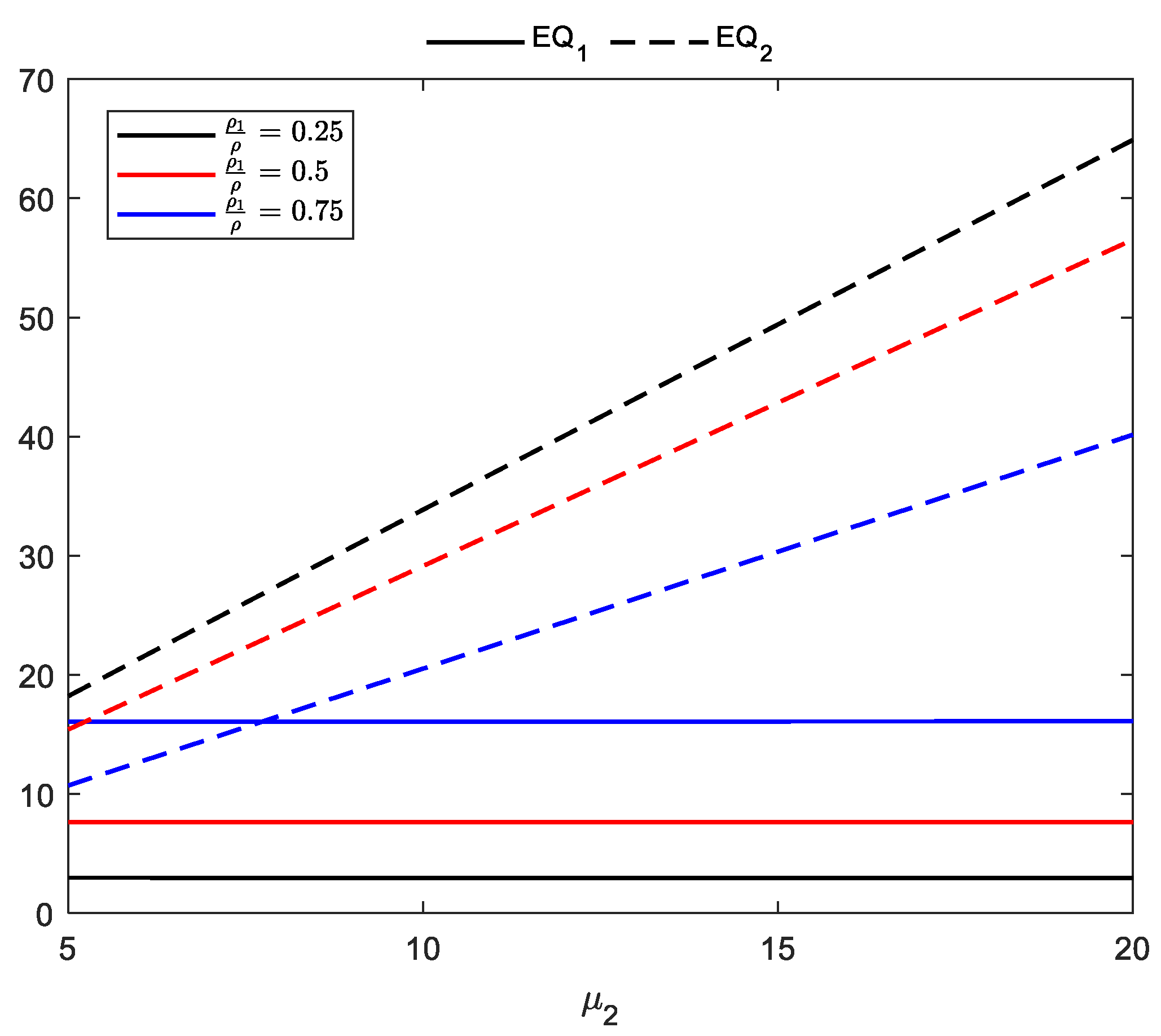
We illustrate the influence of the mean service rate for class-2 customers μ₂ on E[Q₁] and E[Q₂] for a different fraction of class-1 customer load in the overall traffic mix, which can be seen in Figure 1. The other parameters are set to ρ = 0.7, μ₁ = 10, η = 0.4, θ₁ = 2, θ₂ = 3, γ = 50, α_v = 0.4, β_v = 0.2, α_b = 0.1 β_b = 2, q = 0.25.

Figure 1 indicates that the mean length of class-1 customers is constant for varying μ₂ due to the preemptive discipline. The reason is that in the preemptive case, the class-1 customer has absolute priority over the class-2 customer. Therefore, there are no class-2 customers for class-1 customers. The increase in the length of class-2 customers is because λ₂ increases with an increase of μ₂ (since ρ keeps constant), so there will be more class-2 customers in the system.

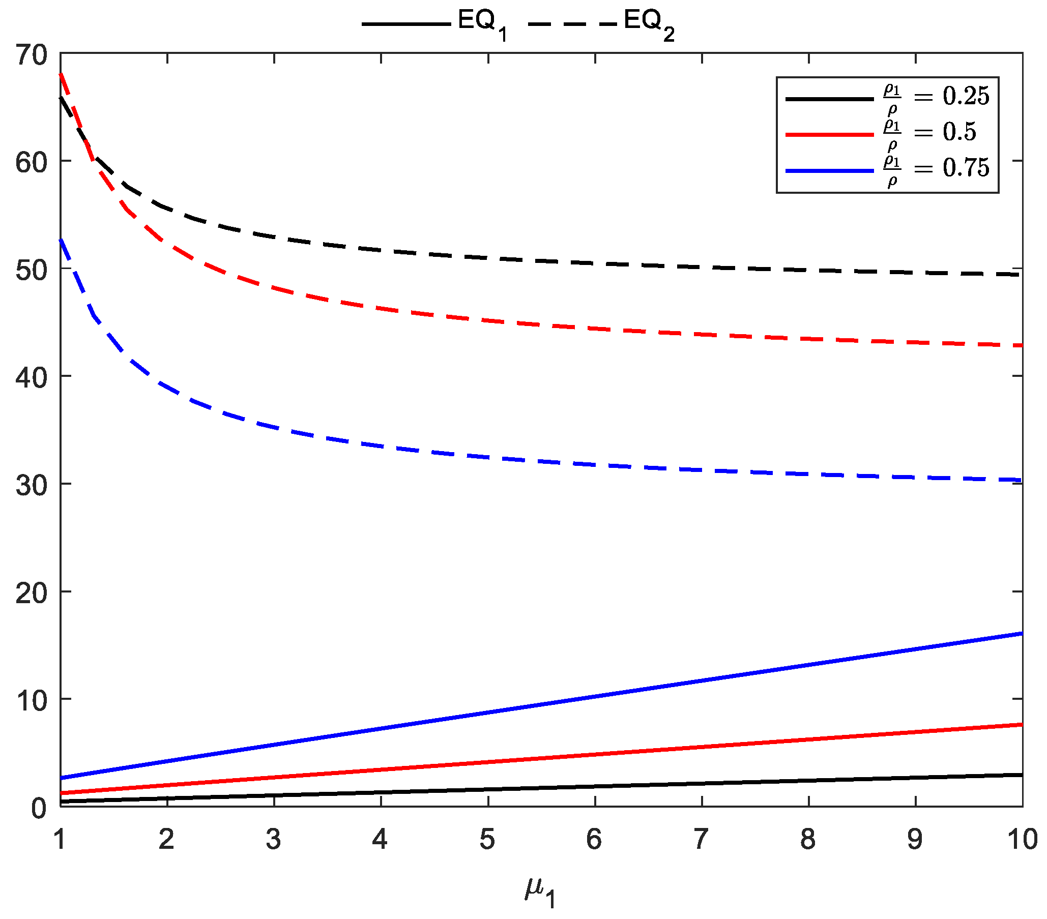
Figure 2 demonstrates the effect of the mean service parameter for class-1 customers μ₁ on E[Q₁] and E[Q₂] for a different fraction of class-1 customer load in the overall traffic mix. The other parameters are set to ρ = 0.7, μ₂ = 15, η = 0.4, θ₁ = 2, θ₂ = 3, γ = 50, α_v = 0.4, β_v = 0.2, α_b = 0.1 β_b = 2, q = 0.25. Figure 2 shows that E[Q₁] increases as μ₁ increases because of increasing λ₁ for increasing μ₁. One also can observe that E[Q₂] decreases as μ₁ increases. A larger μ₁ means a shorter service time for class-1 customers, which results in faster service for class-2 customers because class-1 customers are quickly serviced and leave the system. Hence, E[Q₂] decreases.

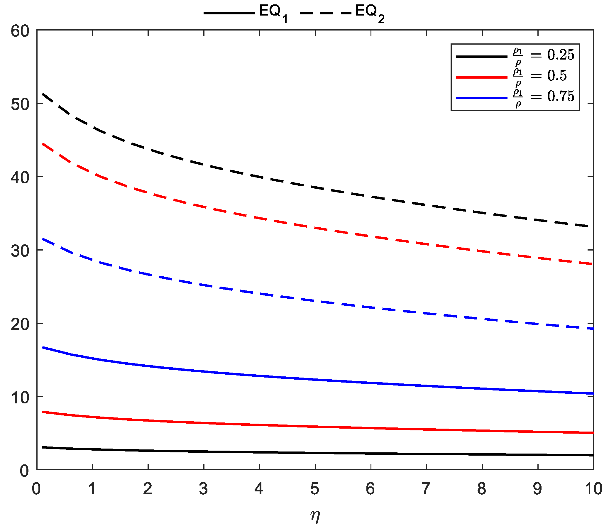
The effect of the vacation parameter η on E[Q₁] and E[Q₂] for a different fraction of class-1 customer load in the overall traffic mix is demonstrated in Figure 3. The other parameters are set to ρ = 0.7, μ₁ = 10, μ₂ = 15, θ₁ = 2, θ₂ = 3, γ = 50, α_v = 0.4, β_v = 0.2, α_b = 0.1, β_b = 2, q = 0.25. One can find from Figure 3 that E[Q₁] and E[Q₂] decrease as η increases, which is because the duration of vacation increases with decreasing η.

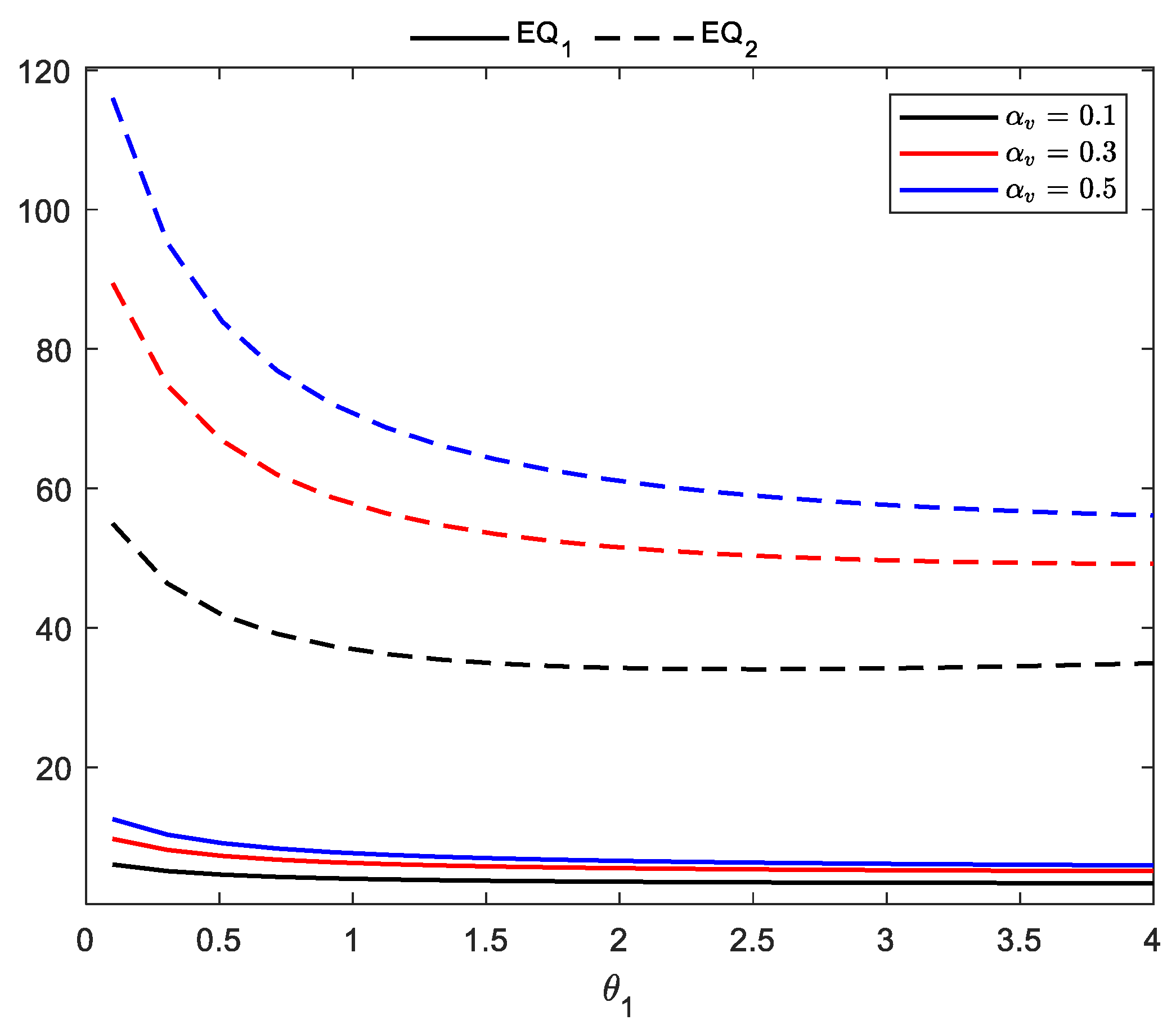
Figure 4 depicts the impact of low service rate θ₁ on E[Q₁] and E[Q₂] for different α_v. The other parameters are set to λ₁ = 4, λ₂ = 6, μ₁ = 10, μ₂ = 15, η = 0.4, θ₂ = 3, γ = 50, β_v = 0.2, α_b = 0.1 β_b = 2, q = 0.25. The mean lengths of each class of customer decrease as θ₁ increases. The effect of θ₁ on E[Q₁] seems to be insignificant when θ₁ is larger. This is due to considering the working vacation interruption policy. At the instant of completing service during vacation duration, if the system is not empty, the server resumes the service rate μ_i. Further, with a decrease in the value of α_v, the mean length of customers for each class reduces. It is intuitive because a reduced number of breakdowns in the server leads to a shorter mean length of customers for each class.

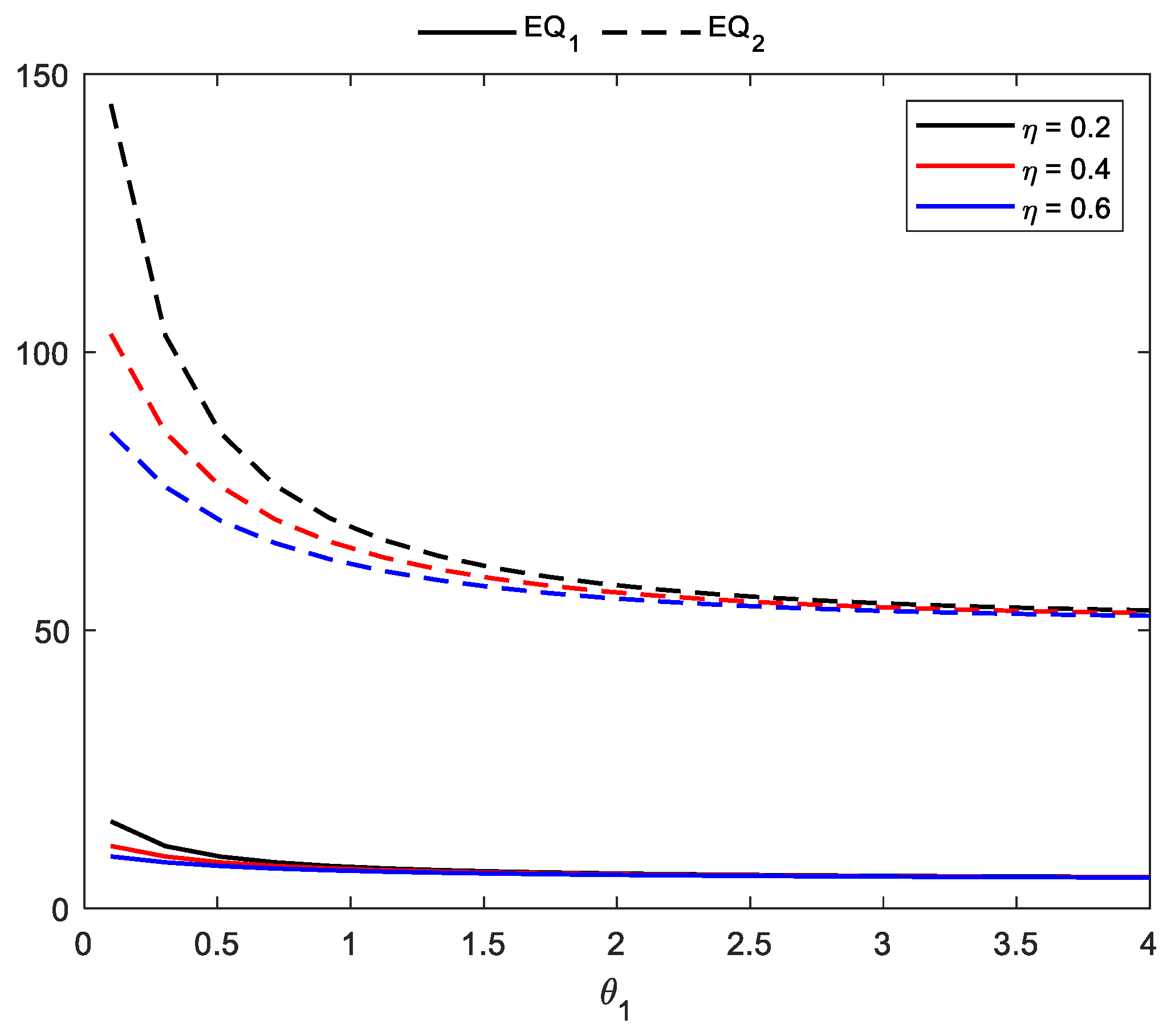
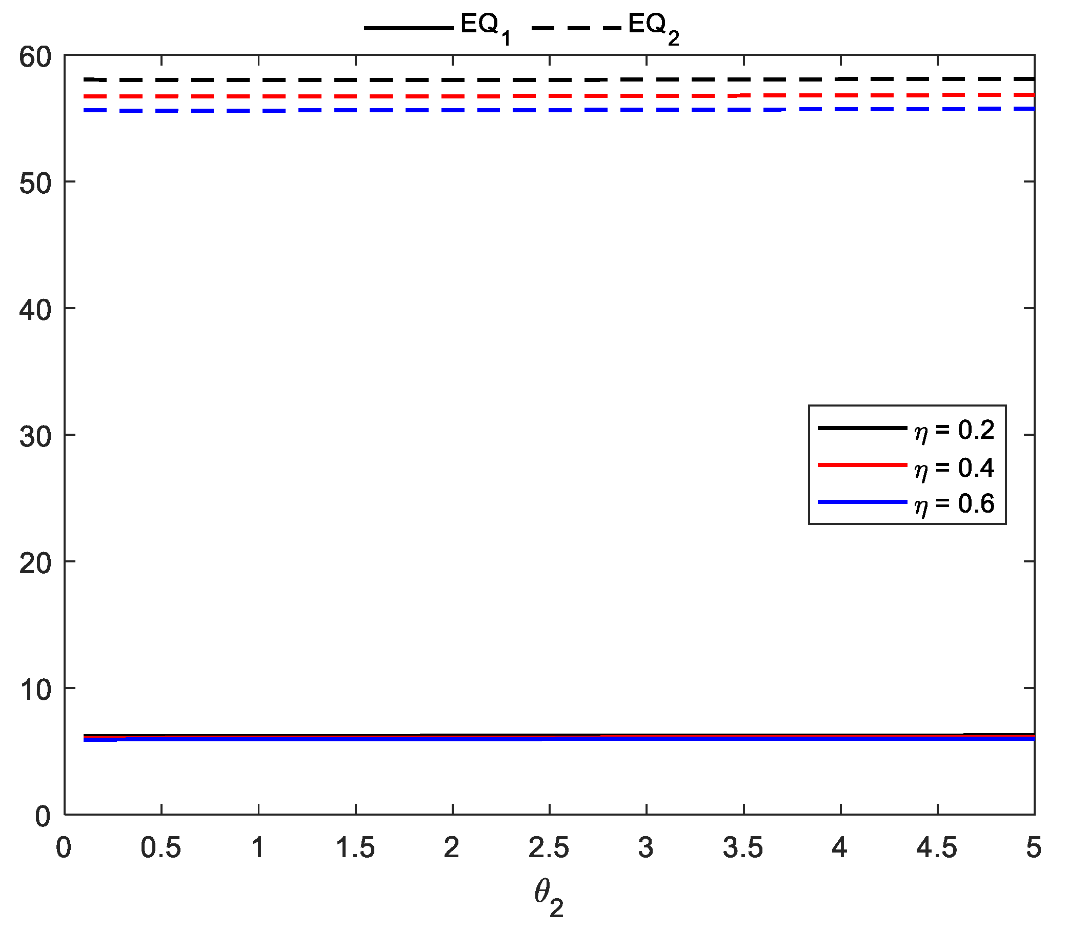
Figure 5 and Figure 6 display the impact of change in the vacation service rate θ₁ and θ₂ on E[Q₁] and E[Q₂] for different η, respectively. The other parameters are set to λ₁ = 4, λ₂ = 6, μ₁ = 10, μ₂ = 15, θ₂ = 3, γ = 50, α_v = 0.4, β_v = 0.2, α_b = 0.1 β_b = 2, q = 0.25. As we find from this figure, E[Q₁] and E[Q₂] decrease as the low-speed service rate increases. It can be seen that when θ₁ is large, the influence of η on E[Q₁] and E[Q₂] is not obvious. Clearly, θ₂ does not affect E[Q₁] and E[Q₂].

5.2. Cost Optimization

The manager may be interested in minimizing operating costs. We here perform a cost optimization in which the decision variable is the vacation rate. Thus, we can mathematically describe the cost optimization as:

Min $CF\left(\eta \right)$

Subject to $\eta >0$

where $CF\left(\eta \right)$ is as given in the previous section and $CF\left(\eta \right)$ is assumed to be a function of η.

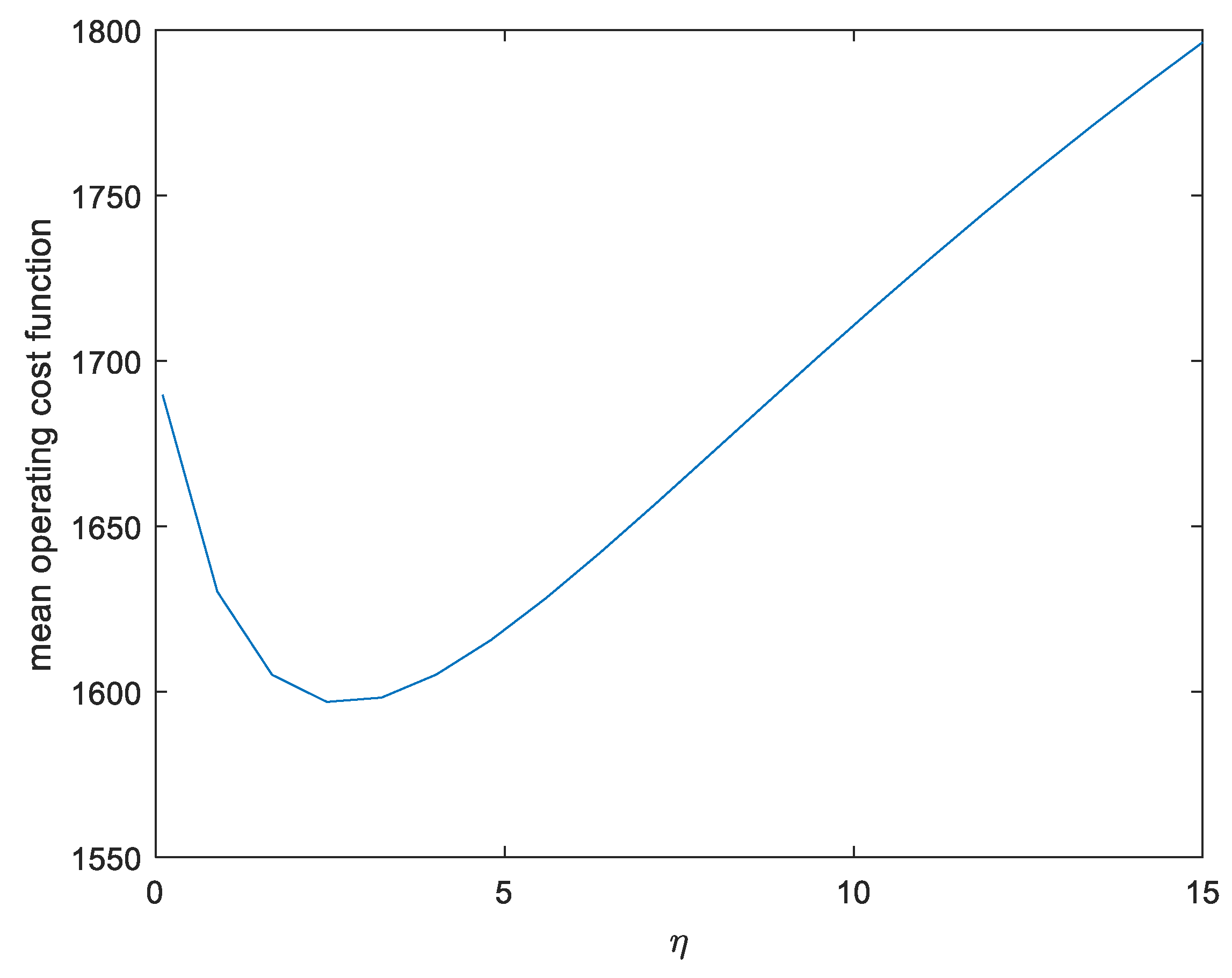
Figure 7 displays how the operating cost function varies with the value of η. The parameter setting in Figure 6 is λ₁ = 2, λ₂ = 3, μ₁ = 10, μ₂ = 15, θ₁ = 2, θ₂ = 3, γ = 50, α_v = 0.3, β_v = 0.1, α_b = 0.2, β_b = 1.25, q = 0.2, r₁ = 40, r₂ = 20, r_s = 800, r_b = 500, r_d = 400, r_v = 200, r_f = 150. From this figure, one can find that an optimal vacation rate exists which minimizes the cost. To solve this cost optimization issue, the particle swarm optimization approach is utilized to search for the optimal value of η. For a review of the particle swarm optimization approach, one can refer to Bonyadi & Michalewicz [29]. The power of this approach lies in its ability to meet performance criteria without prior knowledge of candidate configurations, and the convenience of finding a globally optimal result. Implementing the particle swarm optimization method by MATLAB, we can find the optimal solution ${\eta }^{*}=2.692$ with $CF\left({\eta }^{*}\right)=1596.596$.

5.3. Waiting Time and Cost Analysis

In a queueing system, waiting time is a critical factor. To lessen the mean waiting time or queue length, decision-makers may increase the servers, but this will result in increased mean operating costs. To circumvent this situation, a favourable option is to consider multiple objectives simultaneously. Multi-objective optimization offers the decision-maker with trade-offs between objective functions that can be achieved with feasible solutions. As such, some researchers investigated multi-objective optimization problems within queueing systems [30,31,32]. Hence, in this subsection, we investigate a tri-objective optimization problem with the vacation rate as a decision variable:

Min $CF\left(\eta \right)$,

Min $W_1\left(\eta \right)$,

Min $W_2\left(\eta \right)$,

Subject to $\eta >0$,

where $CF\left(\eta \right)$, $W_1\left(\eta \right)$, and $W_2\left(\eta \right)$ are as given in the previous section and we assume that $CF\left(\eta \right)$, $W_1\left(\eta \right)$, and $W_2\left(\eta \right)$ are a function of η.

Unlike single-objective optimization problems, there is no direct way to define the superiority of one solution over another in multi-objective problems. One of the ways to solve this problem is to apply the notions of Pareto optimality. The solution $y\in X$ is considered a non-dominated Pareto optimal solution if it is not dominated by any other solutions. That is, there does not exist a solution $z\in X$ which satisfies $CF\left(z\right)<CF\left(y\right)$ or $W_1\left(z\right)<W_1\left(y\right)$ or $W_2\left(z\right)<W_2\left(y\right)$.

To search for the optimal solution of a multi-objective problem, many methods have been introduced, such as the multi-objective evolutionary algorithm based on decomposition (MOEA/D), multi-objective particle swarm optimization (MOPSO), and so on. Below, we utilize the MOPSO method to obtain the Pareto optimal frontier. Preliminary codes for this study were obtained from Yarpiz Academic Source Codes and Tutorials (found at http://yarpiz.com/59/ypea121-mopso, accessed on 15 January 2022).

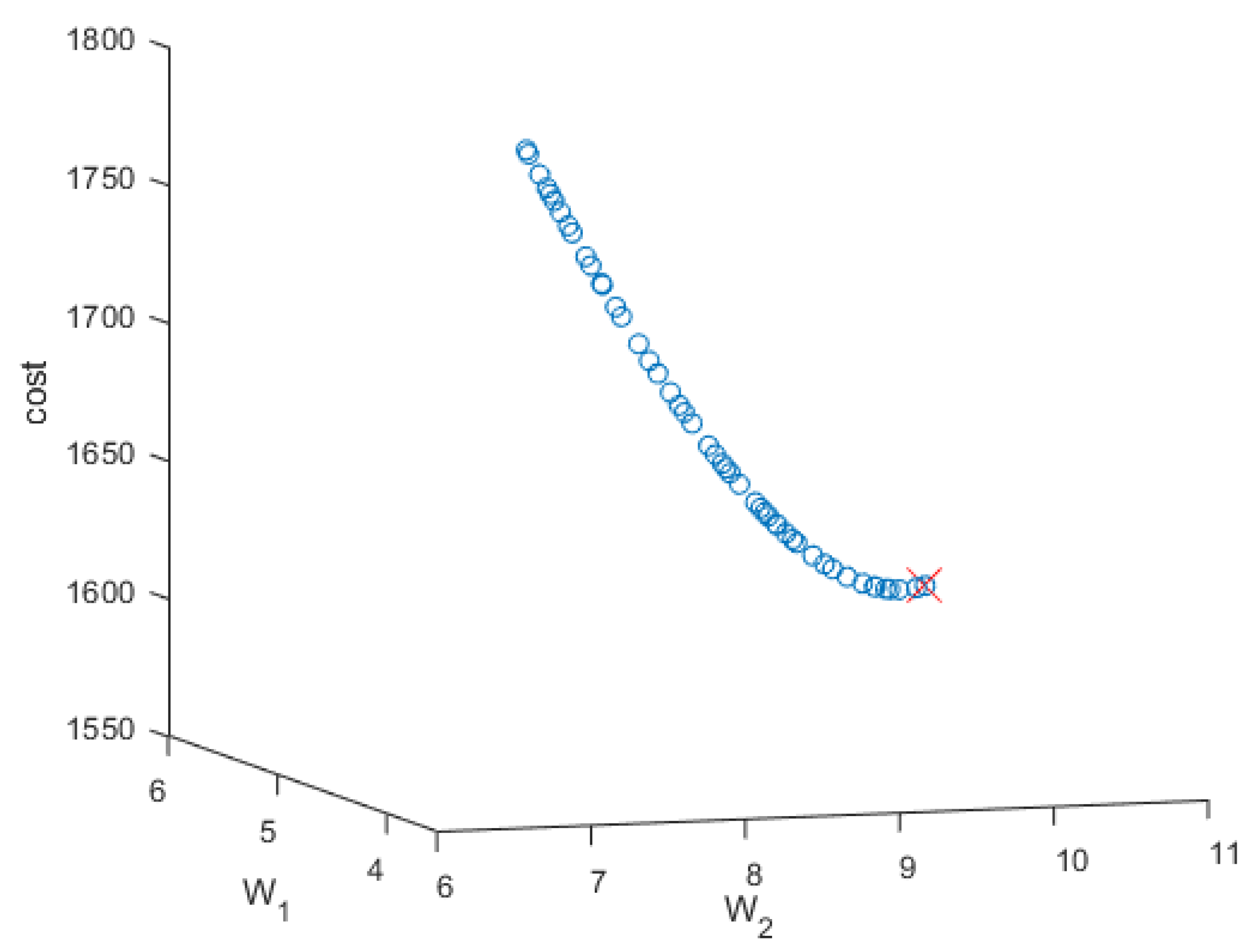
We test the following other parameter settings: λ₁ = 2, λ₂ = 3, μ₁ = 10, μ₂ = 15, θ₁ = 2, θ₂ = 3, γ = 50, α_v = 0.3, β_v = 0.1, α_b = 0.2 β_b = 1.25, q = 0.2, r₁ = 40, r₂ = 20, r_s = 800, r_b = 500, r_d = 400, r_v = 200, r_f = 150. Figure 8 shows the Pareto optimal frontier, indicating that the higher the operating cost, the shorter the mean waiting time of customers for each class. Pareto optimal solutions are summarized in

Table 1. The Pareto optimal solutions.

η*	CF	W1	W2	η*	CF	W1	W2
3.91	1604.039	5.41	10.09	5.04	1619.256	5.13	9.57
2.84	1596.738	5.72	10.65	8.78	1687.794	4.39	8.17
3.18	1597.963	5.62	10.47	7.86	1670.044	4.55	8.48
11.05	1730.026	4.04	7.51	13.36	1770.167	3.73	6.94
2.69	1596.596	5.76	10.74	12.84	1761.468	3.80	7.06
3.35	1599.039	5.57	10.37	12.25	1751.377	3.87	7.20
10.82	1725.915	4.07	7.57	3.67	1601.634	5.48	10.21
7.33	1660.120	4.65	8.66	13.99	1780.379	3.66	6.80
9.51	1701.557	4.27	7.95	14.89	1794.540	3.55	6.60
11.57	1739.440	3.96	7.37	9.07	1693.336	4.34	8.08
13.02	1764.515	3.77	7.01	6.95	1652.857	4.72	8.80
3.44	1599.638	5.54	10.33	8.37	1679.905	4.46	8.31
6.36	1641.983	4.84	9.02	8.62	1684.597	4.42	8.23
7.65	1666.121	4.59	8.55	5.92	1634.116	4.94	9.19
11.61	1740.085	3.96	7.36	10.19	1714.271	4.16	7.75
5.71	1630.279	4.98	9.28	13.66	1774.966	3.70	6.87
5.96	1634.651	4.93	9.18	7.44	1662.199	4.63	8.62
4.25	1608.010	5.33	9.92	6.25	1639.998	4.87	9.06
5.53	1627.281	5.02	9.36	12.04	1747.684	3.90	7.25
13.83	1777.805	3.67	6.83	5.43	1625.650	5.04	9.40
14.34	1786.005	3.61	6.72	7.22	1657.917	4.67	8.70
6.51	1644.585	4.81	8.97	4.58	1612.400	5.24	9.77
3.65	1601.410	5.48	10.22	9.80	1706.97	4.22	7.86
4.76	1615.047	5.20	9.69	6.16	1638.26	4.89	9.10

η* denotes the optimal solution of vacation rate.

. As soon as these results are obtained, the decision-maker needs to choose the best compromise solution out of that set for implementation. This choice is based on the decision maker’s judgment and experience, and there is no right or wrong. For example, the decision-maker can assign his preferences or weighting structure of these three objectives to determine the suitable one. If the weighting structure of these three objectives is set to 0.7, 0.2, and 0.1, for example, then the decision-maker can get the optimal vacation rate found by setting the weights as 2.6906, the corresponding cost is 1596.596, the corresponding mean waiting time of class-1 customers is 5.7642, and the corresponding mean waiting time of class-2 customers is 10.7397.

6. Conclusions Remarks

We have researched unreliable queues under preemptive priority discipline, where vacations can be interrupted. The stationary probability distribution is derived by using the probability generating function approach, and some performance measures are also developed. According to these measures, a mean cost function is constructed, in which the decision variable is the vacation rate. The impact of system parameters is illustrated numerically. Further, we have determined the minimum cost and joint minimum cost and waiting time by using the particle swarm optimization approach and multi-objective particle swarm optimization approach, respectively.

References

- Tian, N.; Zhang, Z.G. Vacation Queueing Models: Theory and Applications; Springer: Boston, MA, USA, 2006. [Google Scholar]
- Ke, J.C.; Wu, C.H.; Zhang, Z.G. Recent developments in vacation queueing models: A short survey. Int. J. Oper. Res. 2010, 7, 3–8. [Google Scholar]
- Servi, L.D.; Finn, S.G. M/M/1 queues with working vacations (M/M/1/WV). Perform. Eval. 2002, 50, 41–52. [Google Scholar] [CrossRef]
- Tian, N.; Li, J.; Zhang, G. Matrix analysis method and working vacation queueing survey. Int. J. Manag. Sci. 2009, 20, 603–633. [Google Scholar]
- Choudhury, G.; Kalita, C.R. An M/G/1 queue with two types of general heterogeneous service and optional repeated service subject to server’s breakdown and delayed repair. Qual. Technol. Quant. Manag. 2018, 15, 622–654. [Google Scholar] [CrossRef]
- Varalakshmi, M.; Chandrasekaran, V.M.; Saravanarajan, M.C. A single server queue with immediate feedback, working vacation and server breakdown. Int. J. Eng. Technol. 2018, 7, 476–479. [Google Scholar]
- Vijayashree, K.V.; Anjuka, A. Stationary analysis of a fluid queue driven by an M/M/1 queue with working vacation. Qual. Technol. Quant. Manag. 2018, 15, 187–208. [Google Scholar] [CrossRef]
- Kempa, W.M.; Kobielnik, M. Transient solution for the queue-size distribution in a finite-buffer model with general independent input stream and single working vacation policy. Appl. Math. Model. 2018, 59, 614–628. [Google Scholar] [CrossRef]
- Suranga Sampath, M.I.G.; Liu, J. Impact of customers’ impatience on an M/M/1 queueing system subject to differentiated vacations with a waiting server. Qual. Technol. Quant. Manag. 2020, 17, 125–148. [Google Scholar] [CrossRef]
- Shekhar, C.; Varshney, S.; Kumar, A. Matrix-geometric solution of multi-server queueing systems with Bernoulli scheduled modified vacation and retention of reneged customers: A meta-heuristic approach. Qual. Technol. Quant. Manag. 2021, 18, 39–66. [Google Scholar] [CrossRef]
- Bouchentouf, A.A.; Guendouzi, A.; Meriem, H.; Shakir, M. Analysis of a single server queue in a multi-phase random environment with working vacations and customers’ impatience. Oper. Res. Decis. 2022, 32, 16–33. [Google Scholar] [CrossRef]
- Bouchentouf, A.A.; Yahiaoui, L.; Kadi, M.; Majid, S. Impatient customers in Markovian queue with Bernoulli feedback and waiting server under variant working vacation policy. Oper. Res. Decis. 2020, 30, 5–28. [Google Scholar] [CrossRef]
- Vadivukarasi, M.; Kalidass, K. Discussion on the transient behavior of single server Markovian multiple variant vacation queues. Oper. Res. Decis. 2021, 31, 123–146. [Google Scholar] [CrossRef]
- Li, J.; Tian, N. The M/M/1 queue with working vacations and vacation interruptions. J. Syst. Sci. Syst. Eng. 2007, 16, 121–127. [Google Scholar] [CrossRef]
- Lee, D.H. Equilibrium balking strategies in Markovian queues with a single working vacation and vacation interruption. Qual. Technol. Quant. Manag. 2019, 16, 355–376. [Google Scholar] [CrossRef]
- Bouchentouf, A.A.; Guendouzi, A.; Majid, S. On impatience in Markovian M/M/1/N/DWV queue with vacation interruption. Croat. Oper. Res. Rev. 2020, 11, 1–37. [Google Scholar] [CrossRef]
- Shekhar, C.; Varshney, S.; Kumar, A. Optimal and sensitivity analysis of vacation queueing system with F-policy and vacation interruption. Arab. J. Sci. Eng. 2020, 45, 7091–7107. [Google Scholar] [CrossRef]
- Vijayashree, K.V.; Ambika, K. An M/M/1 queue subject to differentiated vacation with partial interruption and customer impatience. Qual. Technol. Quant. Manag. 2021, 18, 657–682. [Google Scholar]
- Choudhury, G.; Deka, M. A batch arrival unreliable server delaying repair queue with two phases of service and Bernoulli vacation under multiple vacation policy. Qual. Technol. Quant. Manag. 2018, 15, 157–186. [Google Scholar] [CrossRef]
- Jiang, T.; Xin, B. Computational analysis of the queue with working breakdowns and delaying repair under a Bernoulli-schedule-controlled policy. Commun. Stat. Theory Methods 2019, 48, 926–941. [Google Scholar] [CrossRef]
- Yang, D.Y.; Cho, Y.C. Analysis of the N-policy GI/M/1/K queueing systems with working breakdowns and repairs. Comput. J. 2019, 62, 130–143. [Google Scholar] [CrossRef]
- Zhang, Y.; Wang, J. Strategic joining and information disclosing in Markovian queues with an unreliable server and working vacations. Qual. Technol. Quant. Manag. 2021, 18, 298–325. [Google Scholar] [CrossRef]
- Brandwajn, A.; Begin, T. Multi-server preemptive priority queue with general arrivals and service times. Perform. Eval. 2017, 115, 150–164. [Google Scholar] [CrossRef]
- Wang, J.; Cui, S.; Wang, Z. Equilibrium strategies in M/M/1 priority queues with balking. Prod. Oper. Manag. 2019, 28, 43–62. [Google Scholar] [CrossRef]
- Kim, K. Delay cycle analysis of finite-buffer M/G/1 queues and its application to the analysis of M/G/1 priority queues with finite and infinite buffers. Perform. Eval. 2020, 143, 102133. [Google Scholar] [CrossRef]
- Kim, B.; Kim, J.; Bueker, O. Non-preemptive priority M/M/m queue with servers’ vacations. Comput. Ind. Eng. 2021, 160, 107390. [Google Scholar] [CrossRef]
- Ajewole, O.R.; Mmduakor, C.O.; Adeyefa, E.O.; Okoro, J.O.; Ogunlade, T.O. Preemptive-resume priority queue system with Erlang service distribution. J. Theor. Appl. Inf. Technol. 2021, 99, 1426–1434. [Google Scholar]
- Gao, S.; Zhang, J.; Wang, X. Analysis of a retrial queue with two-type breakdowns and delayed repairs. IEEE Access 2020, 8, 172428–172442. [Google Scholar] [CrossRef]
- Bonyadi, M.R.; Michalewicz, Z. Particle swarm optimization for single objective continuous space problems: A review. Evol. Comput. 2017, 25, 1–54. [Google Scholar] [CrossRef] [PubMed]
- Goodarzi, A.H.; Diabat, E.; Jabbarzadeh, A.; Paquet, M. An M/M/c queue model for vehicle routing problem in multi-door cross-docking environments. Comput. Oper. Res. 2022, 138, 105513. [Google Scholar] [CrossRef]
- Hajipour, V.; Farahani, R.Z.; Fattahi, P. Bi-objective vibration damping optimization for congested location-pricing problem. Comput. Oper. Res. 2016, 70, 87–100. [Google Scholar] [CrossRef]
- Wu, C.H.; Yang, D.Y. Bi-objective optimization of a queueing model with two-phase heterogeneous service. Comput. Oper. Res. 2021, 130, 105230. [Google Scholar] [CrossRef]
Figure 1.
Effect of μ2 on the length of each class of customers.
Figure 2.
Effect of μ1 on the length of each class of customers.
Figure 3.
Effect of η on the length of each class of customers.
Figure 4.
Variation in the length of each class of customers in vacation service rate θ1 for different αv.
Figure 5.
Effect of the vacation service rate θ1 on the length of each class of customers for different η.
Figure 6.
Effect of the vacation service rate θ2 on the length of each class of customers for different η.
Figure 7.
Effect of η on the mean operating cost function.
Figure 8.
Pareto front solutions found by the multi-objective particle swarm optimization algorithm.