
Experimental Evidence of Generation and Reception by a Transluminal Axisymmetric Shear Wave Elastography Prototype

 , , ,
, , , 
Abstract
:1. Introduction
2. Materials and Methods
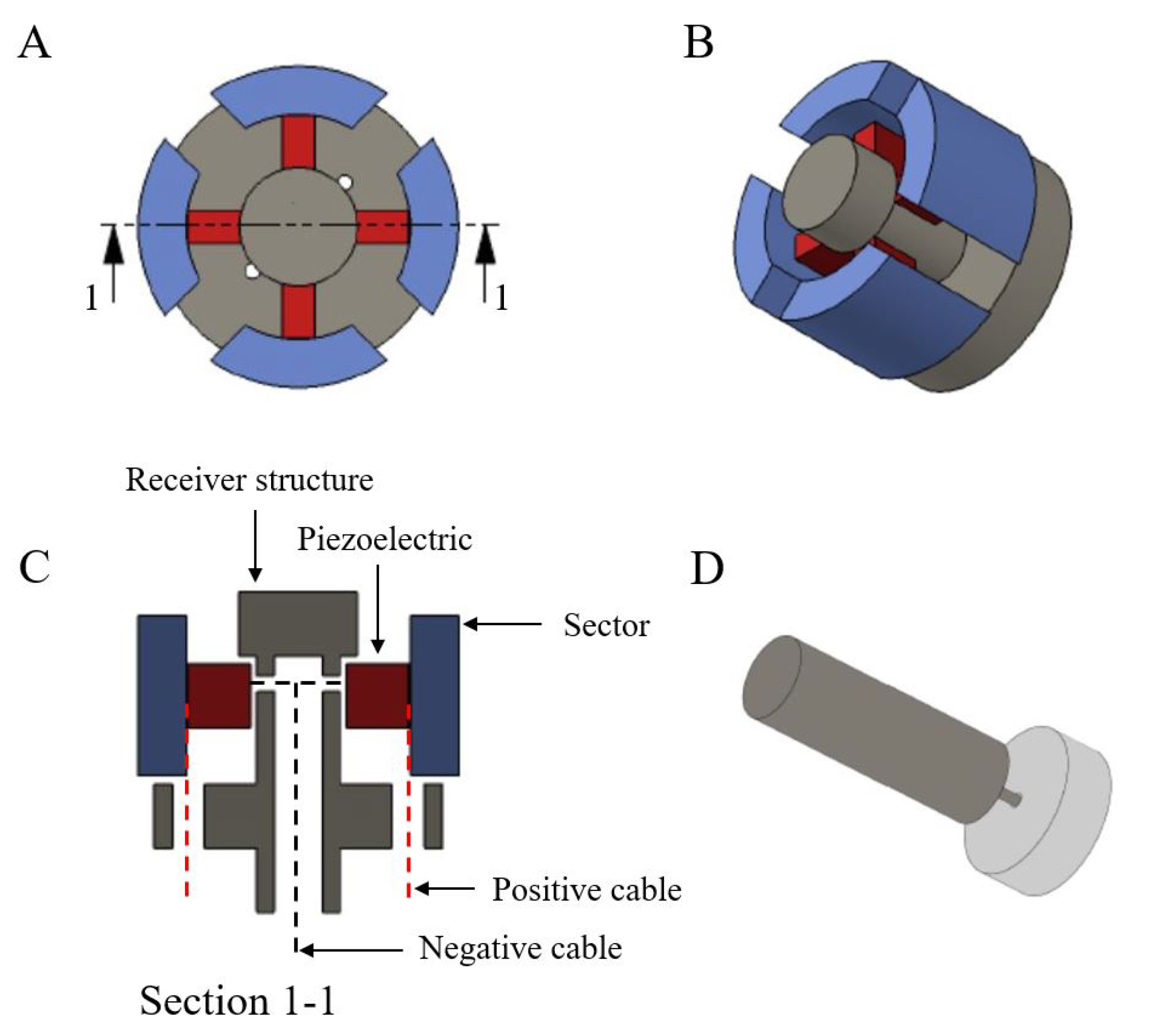
2.1. Transluminal Probe
2.2. Tissue-Mimicking Phantom Fabrication
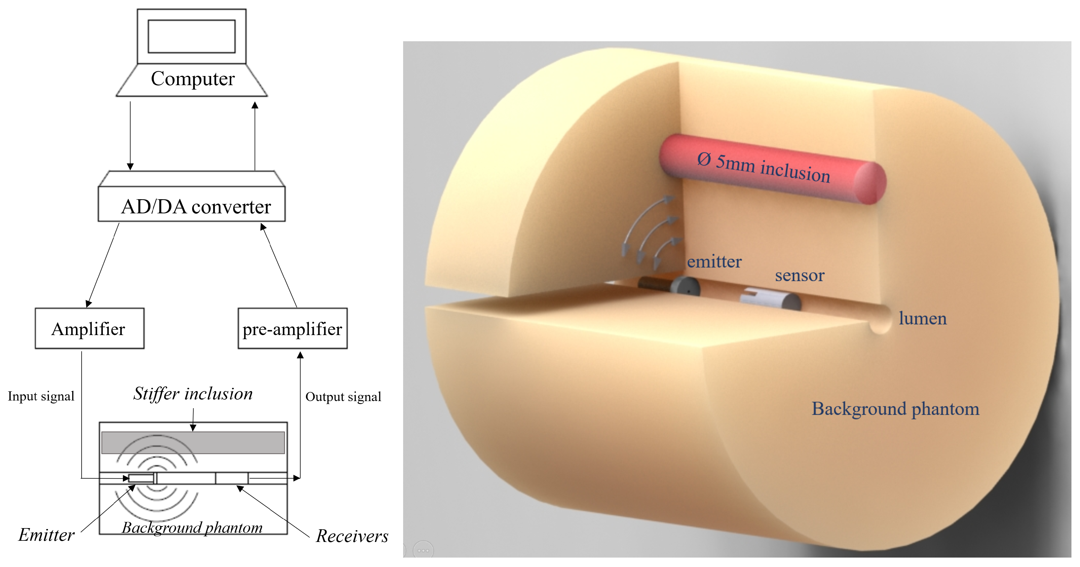
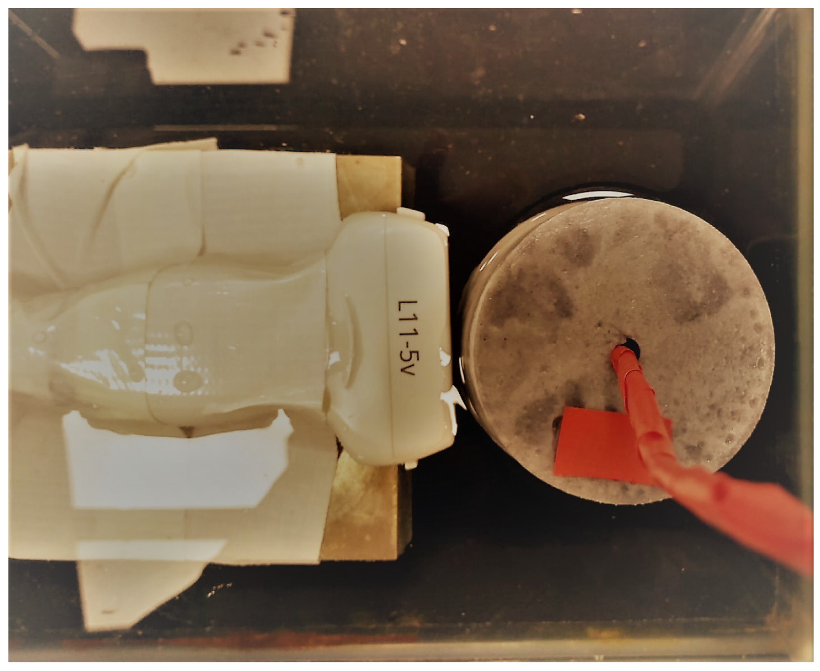
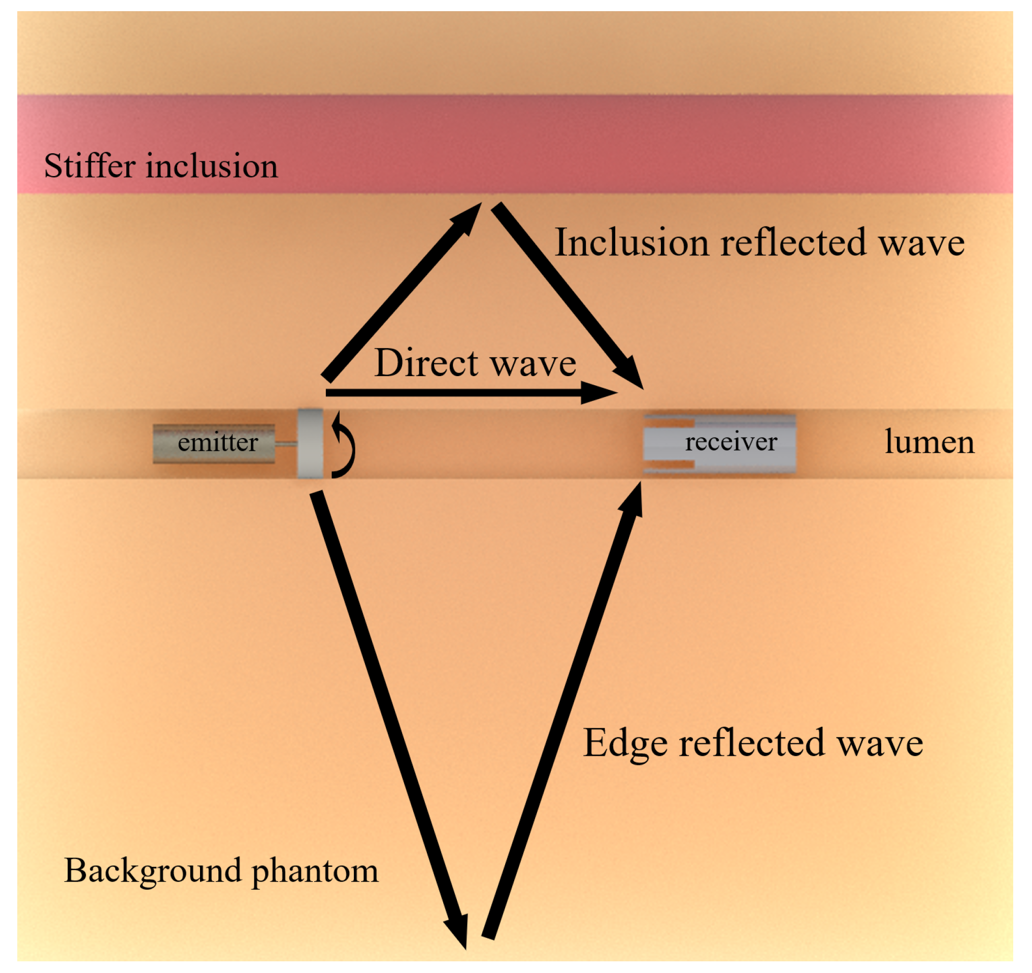
2.3. Transluminal Transmission–Reception (T–R) Tests
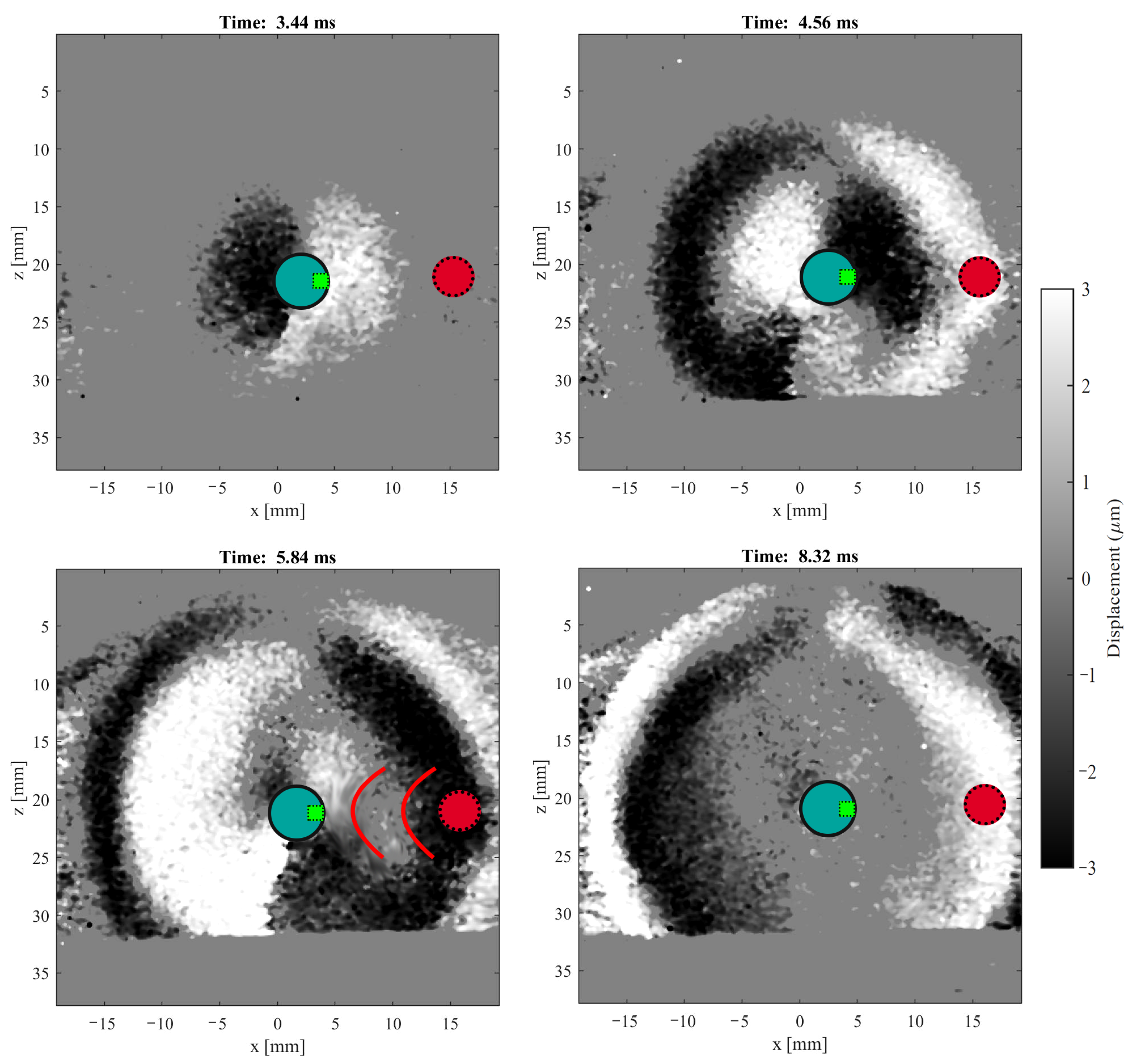
2.4. Ultrafast Imaging for Tracking the Shear Wave Propagation and Characterization of the Shear Wave Speed
3. Results
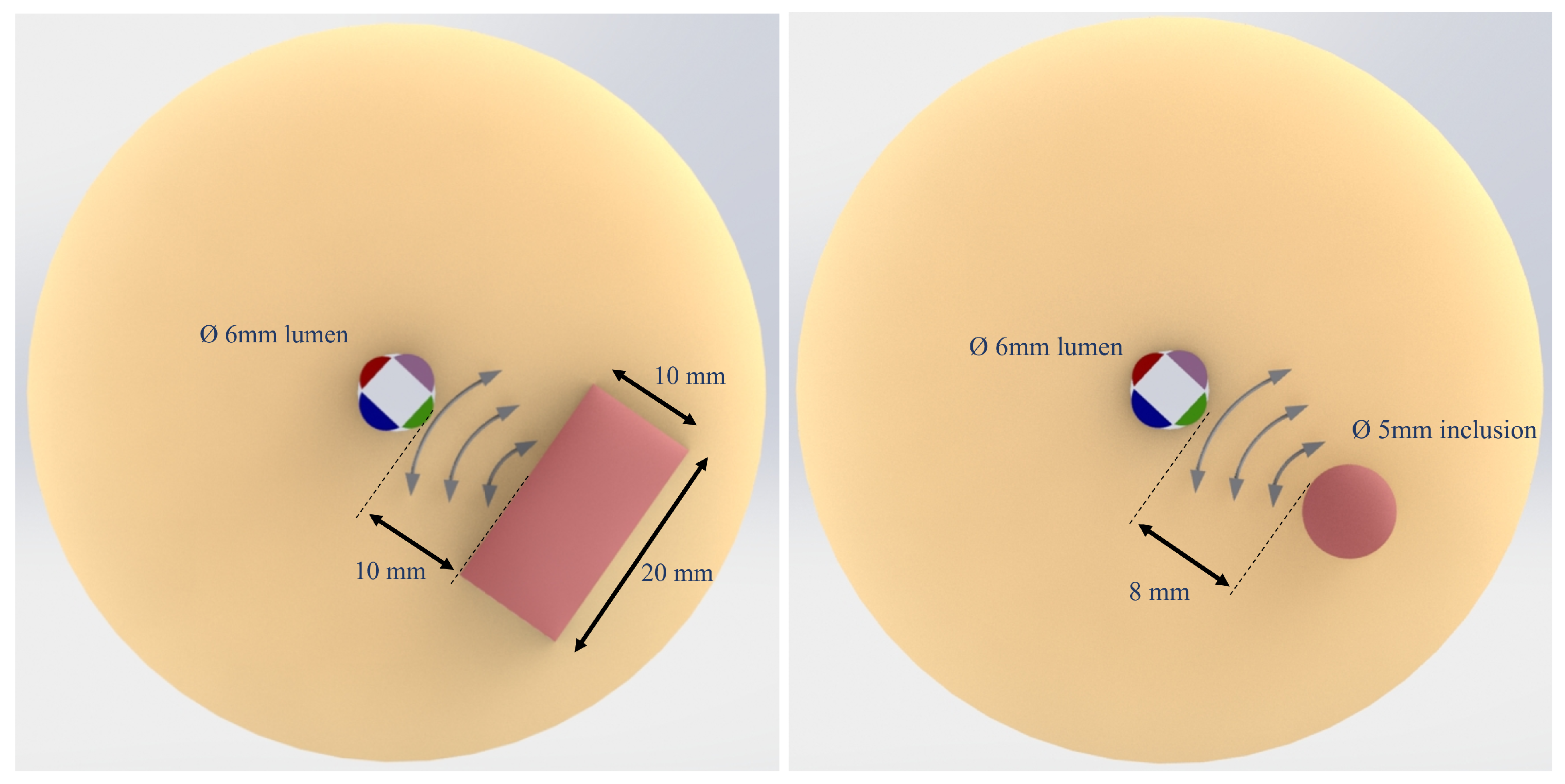
3.1. Estimated Time-of-Flight
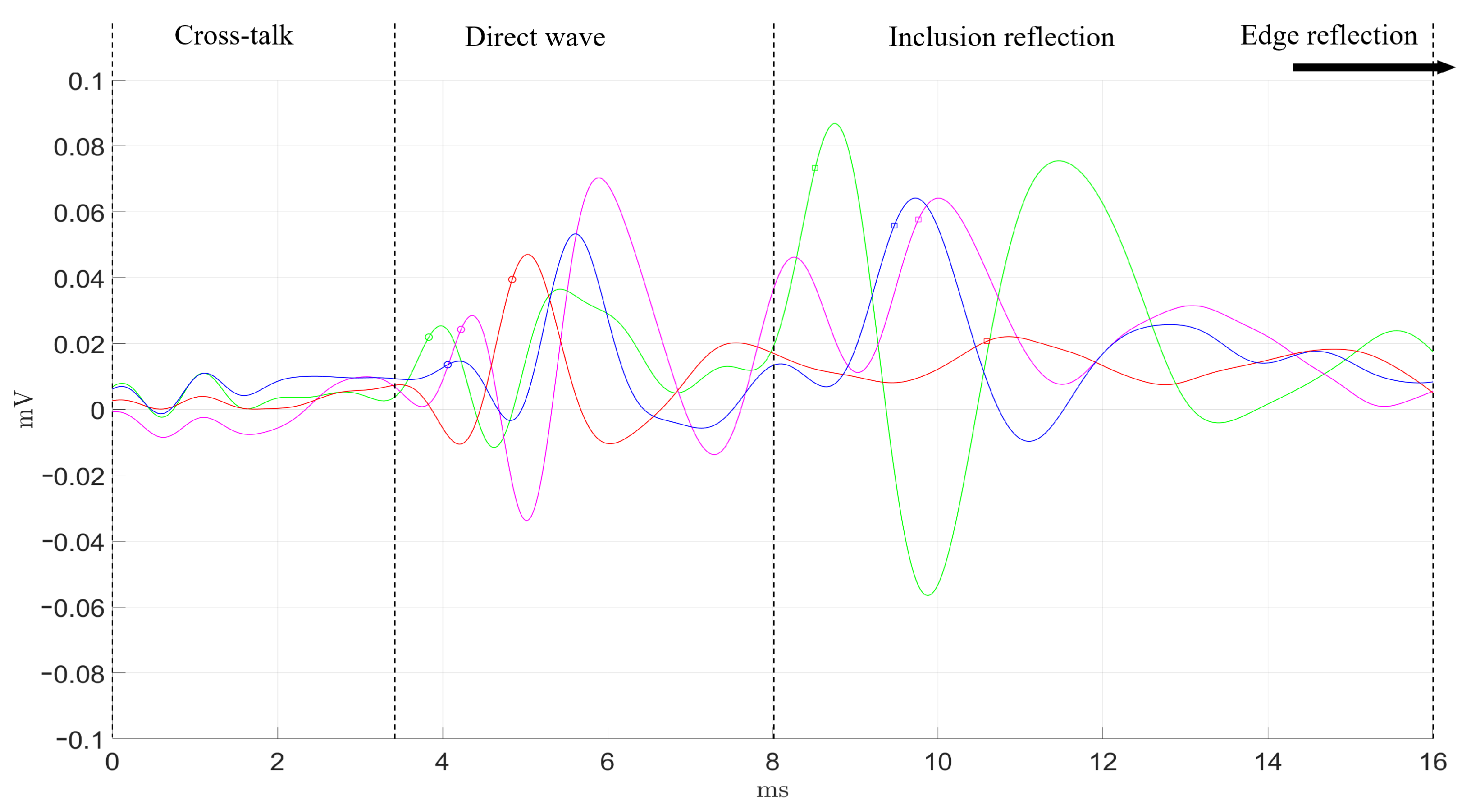
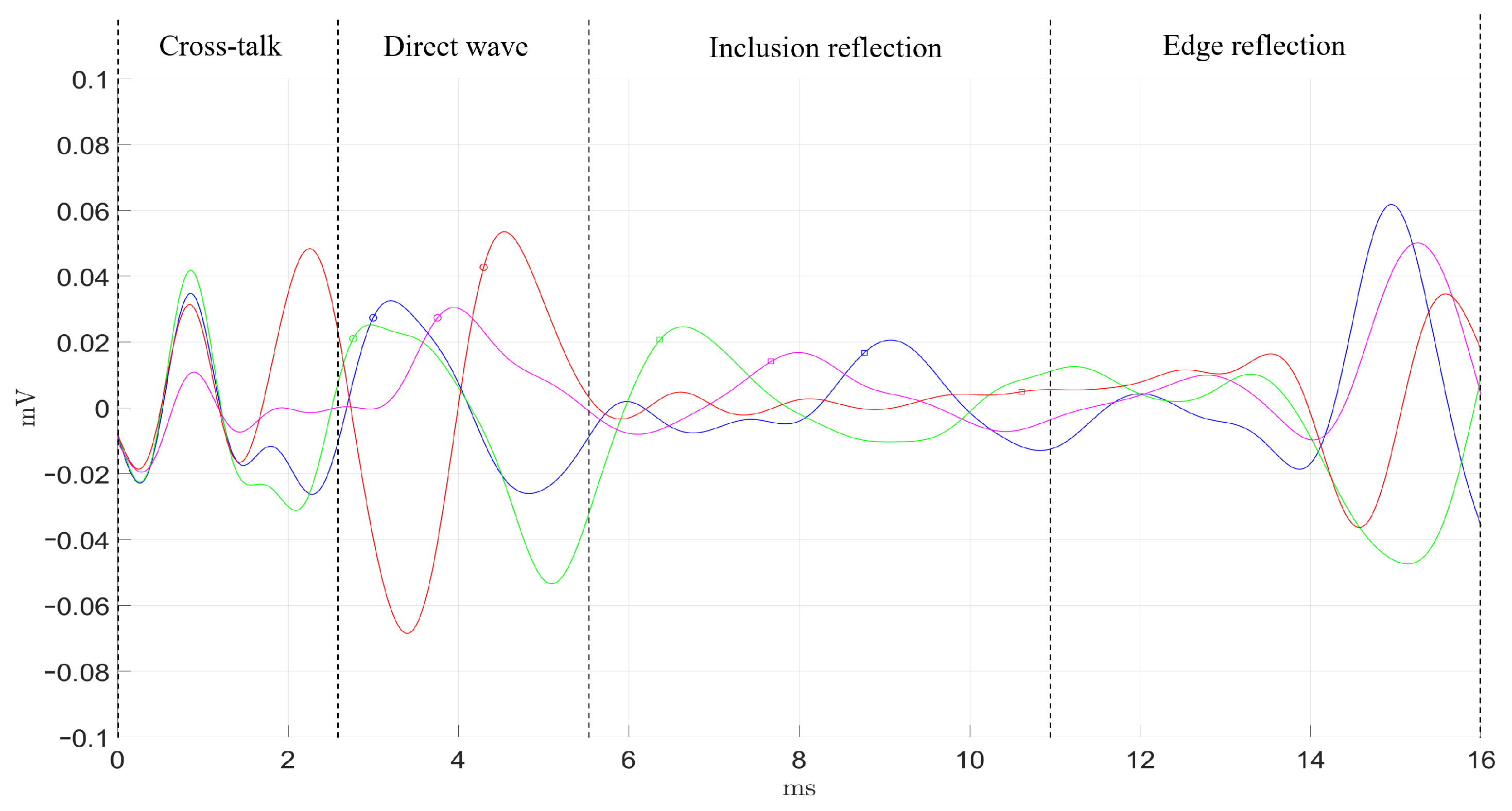
3.2. Transluminal T–R Tests
3.3. Transluminal Wave Propagation Tracking
4. Discussion
Author Contributions
Funding
Acknowledgments
Conflicts of Interest
Abbreviations
| PVA | Polyvinyl Alcohol |
| PLA | Polylactic Acid |
| PRF | Pulse Repetition Frequency |
| SWE | Shear Wave Elastography |
| ARF | Acoustic Radiation Force |
| T–R | Transmission–Reception |
| FFT | Fast Fourier Transform |
References
- Sigrist, R.M.; Liau, J.; Kaffas, A.E.; Chammas, M.C.; Willmann, J.K. Ultrasound Elastography: Review of Techniques and Clinical Applications. Theranostics 2017, 7, 1303–1329. [Google Scholar] [CrossRef] [PubMed]
- Rus, G.; Faris, I.H.; Torres, J.; Callejas, A.; Melchor, J. Why Are Viscosity and Nonlinearity Bound to Make an Impact in Clinical Elastographic Diagnosis? Sensors 2020, 20, 2379. [Google Scholar] [CrossRef] [PubMed]
- Cosgrove, D.; Piscaglia, F.; Bamber, J.; Bojunga, J.; Correas, J.M.; Gilja, O.H.; Klauser, A.S.; Sporea, I.; Calliada, F.; Cantisani, V.; et al. EFSUMB guidelines and recommendations on the clinical use of ultrasound elastography. Part 2: Clinical applications. Ultraschall Med. 2013, 34, 238–253. [Google Scholar]
- Gomez, A.; Rus, G.; Saffari, N. Use of shear waves for diagnosis and ablation monitoring of prostate cancer: A feasibility study. J. Phys. Conf. Ser. 2016, 684, 012006. [Google Scholar] [CrossRef]
- Imtiaz, S. Breast elastography: A new paradigm in diagnostic breast imaging. Appl. Radiol. 2018, 47, 14–19. [Google Scholar]
- Barr, R.G. Future of breast elastography. Ultrasonography 2019, 38, 93–105. [Google Scholar] [CrossRef] [PubMed] [Green Version]
- Sinkus, R.; Lambert, S.; Abd-Elmoniem, K.Z.; Morse, C.; Heller, T.; Guenthner, C.; Ghanem, A.M.; Holm, S.; Gharib, A.M. Rheological determinants for simultaneous staging of hepatic fibrosis and inflammation in patients with chronic liver disease. NMR Biomed. 2018, 31, 1–10. [Google Scholar] [CrossRef] [PubMed]
- Fu, J.; Wu, B.; Wu, H.; Lin, F.; Deng, W. Accuracy of real-time shear wave elastography in staging hepatic fibrosis: A meta-analysis. BMC Med. Imaging 2020, 20, 16. [Google Scholar] [CrossRef] [Green Version]
- Céspedes, E.I.; De Korte, C.L.; Van Der Steen, A.F. Intraluminal ultrasonic palpation: Assessment of local and cross-sectional tissue stiffness. Ultrasound Med. Biol. 2000, 26, 385–396. [Google Scholar] [CrossRef]
- Deleaval, F.; Bouvier, A.; Finet, G.; Cloutier, G.; Yazdani, S.K.; Le Floc’h, S.; Clarysse, P.; Pettigrew, R.I.; Ohayon, J. The Intravascular ultrasound elasticity-palpography technique revisited: A reliable tool for the invivo detection of vulnerable coronary atherosclerotic plaques. Ultrasound Med. Biol. 2013, 39, 1469–1481. [Google Scholar] [CrossRef] [Green Version]
- Ramnarine, K.V.; Garrard, J.W.; Kanber, B.; Nduwayo, S.; Hartshorne, T.C.; Robinson, T.G. Shear wave elastography imaging of carotid plaques: Feasible, reproducible and of clinical potential. Cardiovasc. Ultrasound 2014, 12, 1–9. [Google Scholar] [CrossRef] [PubMed] [Green Version]
- Correas, J.M.; Tissier, A.M.; Khairoune, A.; Vassiliu, V.; Méjean, A.; Hélénon, O.; Memo, R.; Barr, R.G. Prostate cancer: Diagnostic performance of real-time shear-wave elastography. Radiology 2015, 275, 280–289. [Google Scholar] [CrossRef] [PubMed] [Green Version]
- Tyloch, D.; Tyloch, J.; Adamowicz, J.; Juszczak, K.; Ostrowski, A.; Warsiński, P.; Wilamowski, J.; Ludwikowska, J.; Drewa, T. Elastography in prostate gland imaging and prostate cancer detection. Med. Ultrason. 2018, 20, 515–523. [Google Scholar] [CrossRef] [PubMed]
- Yang, Y.; Zhao, X.; Shi, J.; Huang, Y. Value of shear wave elastography for diagnosis of primary prostate cancer: A systematic review and meta-analysis. Med. Ultrason. 2019, 21, 382–388. [Google Scholar] [CrossRef]
- Arani, A.; Plewes, D.; Chopra, R. Transurethral prostate magnetic resonance elastography: Prospective imaging requirements. Magn. Reson. Med. 2011, 65, 340–349. [Google Scholar] [CrossRef]
- Masso, P.; Callejas, A.; Melchor, J.; Molina, F.S.; Rus, G. In Vivo Measurement of Cervical Elasticity on Pregnant Women by Torsional Wave Technique: A Preliminary Study. Sensors 2019, 19, 3249. [Google Scholar] [CrossRef] [Green Version]
- Callejas, A.; Gomez, A.; Melchor, J.; Riveiro, M.; Massó, P.; Torres, J.; López-López, M.T.; Rus, G. Performance study of a torsional wave sensor and cervical tissue characterization. Sensors 2017, 17, 2078. [Google Scholar] [CrossRef]
- Callejas, A.; Gomez, A.; Faris, I.H.; Melchor, J.; Rus, G. Kelvin-Voigt Parameters Reconstruction of Cervical Tissue-Mimicking Phantoms Using Torsional Wave Elastography. Sensors 2019, 19, 3281. [Google Scholar] [CrossRef] [Green Version]
- Callejas, A.; Melchor, J.; Faris, I.H.; Rus, G. Viscoelastic model characterization of human cervical tissue by torsional waves. J. Mech. Behav. Biomed. Mater. 2021, 115, 104261. [Google Scholar] [CrossRef]
- Saffari, N.; Rus, G.; Gomez, A.; Sanchez, E. Transluminal Device and Procedure for the Mechanical Characterization of Structures. Patent No. ES2687485A1-PCT/ES2018/070243, 26 March 2018. [Google Scholar]
- Gomez, A. Transurethral Shear Wave Elastography for Prostate Cancer. Ph.D. Thesis, University College London, London, UK, 2018. [Google Scholar]
- Czernuszewicz, T.J.; Homeister, J.W.; Caughey, M.C.; Farber, M.A.; Fulton, J.J.; Ford, P.F.; Marston, W.A.; Vallabhaneni, R.; Nichols, T.C.; Gallippi, C.M. Non-invasive in vivo characterization of human carotid plaques with acoustic radiation force impulse ultrasound: Comparison with histology after endarterectomy. Ultrasound Med. Biol. 2015, 41, 685–697. [Google Scholar] [CrossRef] [Green Version]
- Barr, R.G.; Memo, R.; Schaub, C.R. Shear wave ultrasound elastography of the prostate: Initial results. Ultrasound Q. 2012, 28, 13–20. [Google Scholar] [CrossRef] [PubMed]
- Woo, S.; Suh, C.H.; Kim, S.Y.; Cho, J.Y.; Kim, S.H. Shear-wave elastography for detection of prostate cancer: A systematic review and diagnostic meta-analysis. Am. J. Roentgenol. 2017, 209, 806–814. [Google Scholar] [CrossRef] [PubMed]
- Melchor, J.; Muñoz, R.; Rus, G. Torsional ultrasound sensor optimization for soft tissue characterization. Sensors 2017, 17, 1402. [Google Scholar] [CrossRef] [PubMed] [Green Version]
- Sarvazyan, A.P.; Urban, M.W.; Greenleaf, J.F. Acoustic Waves in Medical Imaging and Diagnosis. Ultrasound Med. Biol. 2013, 39, 1133–1146. [Google Scholar] [CrossRef] [PubMed] [Green Version]
- Woo, S.; Kim, S.Y.; Cho, J.Y.; Kim, S.H. Shear wave elastography for detection of prostate cancer: A preliminary study. Korean J. Radiol. 2014, 15, 346–355. [Google Scholar] [CrossRef] [PubMed] [Green Version]
- Zhang, M.; Fu, S.; Zhang, Y.; Tang, J.; Zhou, Y. Elastic modulus of the prostate: A new non-invasive feature to diagnose bladder outlet obstruction in patients with benign prostatic hyperplasia. Ultrasound Med. Biol. 2014, 40, 1408–1413. [Google Scholar] [CrossRef] [PubMed]
- Fromageau, J.; Brusseau, E.; Vray, D.; Gimenez, G.; Delachartre, P. Characterization of PVA cryogel for intravascular ultrasound elasticity imaging. IEEE Trans. Ultrason. Ferroelectr. Freq. 2003, 50, 1318–1324. [Google Scholar] [CrossRef]
- Faris, I.H.; Melchor, J.; Callejas, A.; Torres, J.; Rus, G. Viscoelastic Biomarkers of Ex Vivo Liver Samples via Torsional Wave Elastography. Diagnostics 2020, 10, 111. [Google Scholar] [CrossRef] [Green Version]
- Loupas, T.; Powers, J.; Gill, R.W. An axial velocity estimator for ultrasound blood flow imaging, based on a full evaluation of the Doppler equation by means of a two-dimensional autocorrelation approach. IEEE Trans. Ultrason. Ferroelectr. Freq. 1995, 42, 672–688. [Google Scholar] [CrossRef]
- Palmeri, M.L.; Wang, M.H.; Dahl, J.J.; Frinkley, K.D.; Nightingale, K.R. Quantifying hepatic shear modulus in vivo using acoustic radiation force. Ultrasound Med. Biol. 2008, 34, 546–558. [Google Scholar] [CrossRef] [Green Version]
- Johnson, B.; Campbell, S.; Campbell-Kyureghyan, N. The differences in measured prostate material properties between probing and unconfined compression testing method. Med. Eng. Phys. 2020, 80, 40–51. [Google Scholar] [CrossRef] [PubMed]


| Background | Inclusion | |
|---|---|---|
| PVA | 15% | 20% |
| Graphite powder | 0.5% | 0.5% |
| Cellulose | 0.5% | - |
| Freezing–thawing cycles | 1 | 2 |
| Phantoms A and B | Shear Wave Speed (m/s) |
|---|---|
| Background | 3.20 ± 0.18 |
| Inclusion | 7.31 ± 0.16 |
| Phantom A | Phantom B | |||
|---|---|---|---|---|
| Distance (mm) | Time (ms) | Distance (mm) | Time (ms) | |
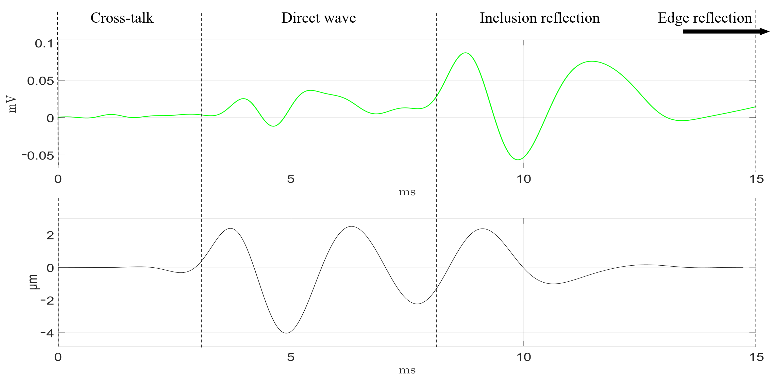
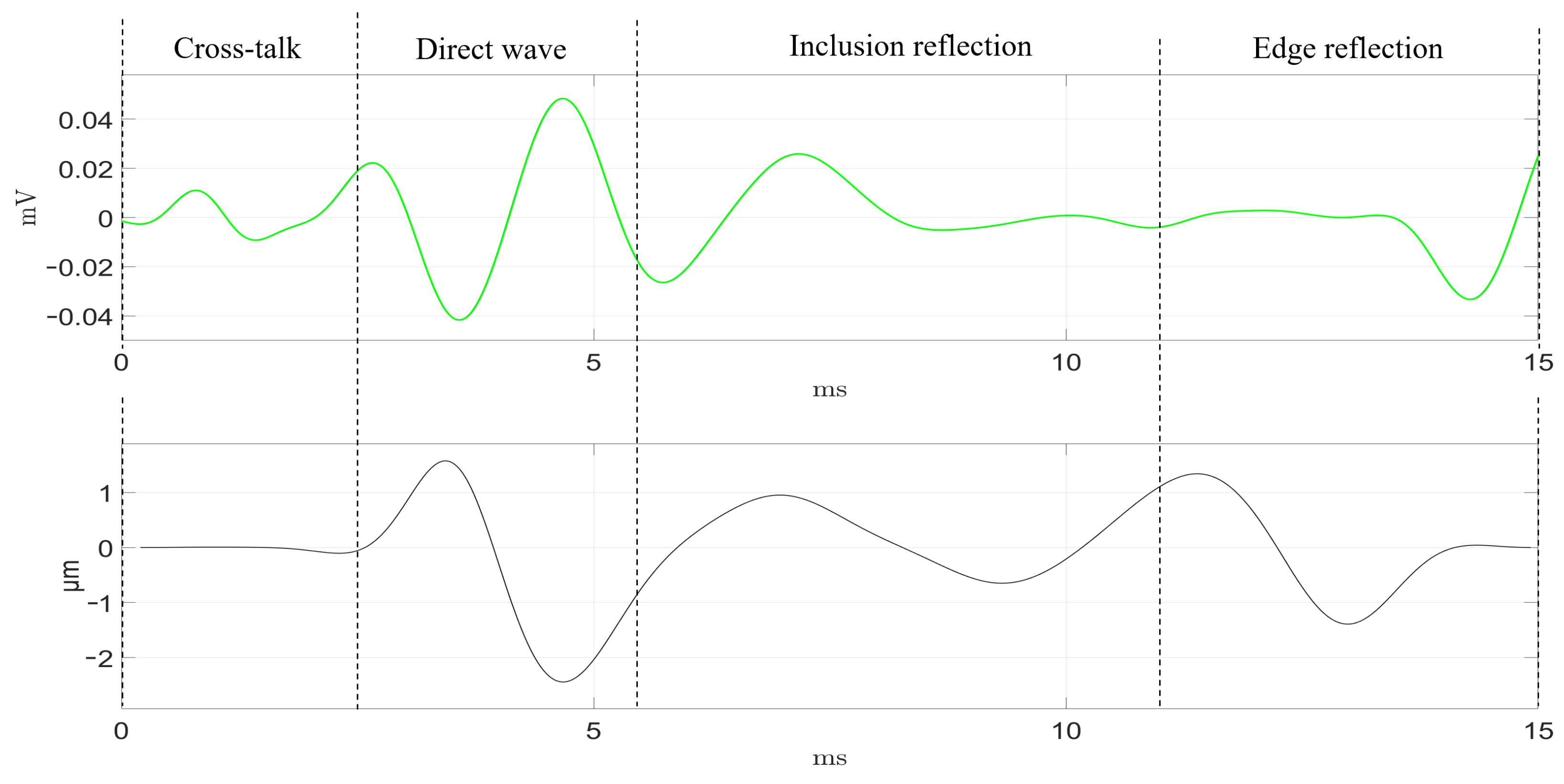
| Direct wave | 10 | 3.1 | 8 | 2.5 |
| Inclusion reflected wave | 25 | 8 | 18 | 5.6 |
| Edge reflected wave | 55 | 17 | 35 | 10.9 |
Publisher’s Note: MDPI stays neutral with regard to jurisdictional claims in published maps and institutional affiliations. |
© 2021 by the authors. Licensee MDPI, Basel, Switzerland. This article is an open access article distributed under the terms and conditions of the Creative Commons Attribution (CC BY) license (https://creativecommons.org/licenses/by/4.0/).
Share and Cite
Gomez, A.; Hurtado, M.; Callejas, A.; Torres, J.; Saffari, N.; Rus, G. Experimental Evidence of Generation and Reception by a Transluminal Axisymmetric Shear Wave Elastography Prototype. Diagnostics 2021, 11, 645. https://doi.org/10.3390/diagnostics11040645
Gomez A, Hurtado M, Callejas A, Torres J, Saffari N, Rus G. Experimental Evidence of Generation and Reception by a Transluminal Axisymmetric Shear Wave Elastography Prototype. Diagnostics. 2021; 11(4):645. https://doi.org/10.3390/diagnostics11040645
Chicago/Turabian StyleGomez, Antonio, Manuel Hurtado, Antonio Callejas, Jorge Torres, Nader Saffari, and Guillermo Rus. 2021. "Experimental Evidence of Generation and Reception by a Transluminal Axisymmetric Shear Wave Elastography Prototype" Diagnostics 11, no. 4: 645. https://doi.org/10.3390/diagnostics11040645