Non-Linear Diffusion and Power Law Properties of Heterogeneous Systems: Application to Financial Time Series

1
Santa Fe Institute, 1399 Hyde Park Road, Santa Fe, NM 87501, USA
2
Instituto de Investigaciones Filosóficas, Bulnes 642, Buenos Aires 1176, Argentina
3
Facultad de Ingeniería y Tecnología, Universidad San Sebastián, Lota 2465, Santiago 7510157, Chile
Entropy 2018, 20(9), 649; https://doi.org/10.3390/e20090649
Submission received: 13 June 2018
/
Revised: 11 August 2018
/
Accepted: 12 August 2018
/
Published: 30 August 2018
(This article belongs to the Special Issue Power Law Behaviour in Complex Systems)
Abstract
:In this work, we show that it is possible to obtain important ubiquitous physical characteristics when an aggregation of many systems is taken into account. We discuss the possibility of obtaining not only an anomalous diffusion process, but also a Non-Linear diffusion equation, that leads to a probability distribution, when using a set of non-Markovian processes. This probability distribution shows a power law behavior in the structure of its tails. It also reflects the anomalous transport characteristics of the ensemble of particles. This ubiquitous behavior, with a power law in the diffusive transport and the structure of the probability distribution, is related to a fast fluctuating phenomenon presented in the noise parameter. We discuss all the previous results using a financial time series example.
1. Introduction
In recent years, many papers have been written focusing on the study of anomalous collective motions and particularities on probability distributions. In fact, when revising the work done in this area, it is possible to identify different lines of research such as: granular systems [1], turbulence [2], financial processes [3], social dynamics [4,5], among others. We could say that the ubiquitous characteristics that in principle are present in the systems under study have two remarkable properties: power law behavior in the structure of its distribution and dynamic characteristics of a system of many particles with anomalous diffusion (i.e., a power law behavior in its diffusion). The first characteristic occurs in a wide variety of physical, biological and artificial phenomena. Some of these are as dissimilar as the occurrence of the frequency in the use of words, the abundance in the size of biological species, the size of vortices in turbulences, etc. Along with this, it is interesting to note, as we mentioned before, that the characteristics associated with the collective movement of some of these systems, where the second moment, i.e., , being the value for the exponent where the system behaves in a normal way, is the typical quantity to be studied [6].
In this contribution, we will describe particular features at the microscopic level of the system, and how they will impact on the macroscopic characteristics of such behaviors, focusing on a financial time series example. We will first write about the evolution equation of a particle (i.e., a microscopic description), using a Langevin formalism characterized by a stochastic integro–differential equation. Then, we will use a set of similar microscopical systems, to describe the properties of the macroscopical systems (i.e., macroscopic laws). We will arrive to a highly Non-Linear Fokker–Planck equation that was study in relation of nonadditive entropies and complex Systems [7,8]. It has been noticed that the last remark applies in situations where the phase space is partly visited [9]. This approach applies to may situations, as reported elsewhere (see for example [10,11,12] and references therein).
It is important to mention that a central part of our analysis is based on the average of a fluctuating quantity, in an unbalanced equilibrium state of the macroscopical system. The parts that compose this system are cells, or networks of cells, that are characterized to be in a local equilibrium, and can be treated as a collection of similar (or equivalent) particles following the same microscopic dynamics. In that way, we can see the natural emergence of power laws on a compound of mixed complex systems [13].
2. Microscopic Dynamics
Let us start the presentation by studying the microscopic dynamics of a Brownian particle, where dissipation is described by a memory kernel . This considers the history of the individual process of the particle (remember that the Brownian particle is influenced by an external noise, which gives unique characteristics to the realization, for each run of the model or trajectory of each particle, for an experiment in real physical systems). The stochastic integro–differential equation reads as follows [21,22]
In the previous equation, characterizes a Gaussian long–range correlated noise. M is the mass associated with the particle and is a dissipative kernel. We have formally denoted with a possible cut–off. For the stochastic term of the equation, we choose as such it has the following properties
with . The parameter for the coupling strength with the complex bath is . A microscopic random–matrix model was applied in the study of anomalous diffusions [23,24], used to calculate the kernel . Then, the (dissipative) kernel is defined by
In this equation, is related with the complexity of the bath. Notice that for non–integer values of , the bath is called fractal [25]. The behavior of the spectral density is characterized by when the regime is non-Ohmic [24]. It is also important to mention that if the Riemann–Liouville fractional derivative is introduced
with [26,27], we can write and equivalente equation for Equation (1) as
which is a fractional Langevin equation. The previous fractional Langevin equation describes the subdiffusion, for , and the superdiffusion regime for . We have also defined as follows [28]
3. Power Law Behavior in the Movement of Ensemble of Particles
We can obtain several dynamical properties from the ensemble of particles, particularly the position of the particle (its distribution) at any time can be calculated via
i.e., the marginal probability distribution. In this equation we observe that . As usual in the case of Gaussian noises the joint probability distribution can be calculated using only a few cumulants [6]. Then, using the second moment
we can calculate the probability distribution . In the previous equation is known as the generalized Mittag–Leffler function [29].
We can observe the second moment in
that shows an anomalous behavior [30], which we explicitly identify with a power law, with .
From the general previous analysis, we can re-obtain the asymptotic limit for , the classical diffusive transport of the Ornstein–Uhlenbeck process [31]. The evolution for the asymptotic processes corresponds to a diffusion equation, also studied in [32]
The last equation can be linked with the fractional Brownian motion (fBm) process [33], see also [34,35,36,37]. This can be done when identifying with , so is the one time probability distribution of the fBm.
The solution for the last equation in the marginal regime can be written as
4. A Marginalization of Weakly Coupled Systems
In the final equation of the last section, we have explicitly noted parameter b, i.e., we wrote . This conditional distribution assigns an event a probability given a particular value of b. As the reader can guess, when doing a simple average over a distribution we can obtain the distribution . The resulting distribution, noted here as , will be the result of a simple integration
It is worth noting that the distribution will be determined by the specific spatiotemporal dynamics of the entire system under consideration. For physical systems it is defined on a positive support. One case, among the variety of possible elections, occurs when nearly independent microscopic Gaussian random variables, with average zero, contribute in an additive way to the final dynamics of the system. If b is given by the sum
then, the distribution of this stochastic variable follows
which is called Gamma-distribution of order n.
Now, if we consider the inverse of b (the “temperature” for physical systems), the distribution that naturally arises is the inverse Gamma-distribution
Also, it is important to mention some important contributions to the field when considering multiplicative noises. Following these lines, if we have a random variable which formally can be expressed by
where are n random variables, invoking the Central Limit Theorem, we can find that the distribution follows a log-normal distribution
with
with m and as mean and variance.
These types of distributions give rise to the distribution with a slow decay, sometimes more complex than the simple power law behavior [38].
Important analytical results can be seen if we perform the marginalization over Equation (9) using the distribution written in Equation (13). We can find the evolution equation for the complete system as
where the diffusion parameter follows
The distribution that satisfies this equation presents a clear power law behavior
as can be seen, this characteristic is more critical for larger values of x.
5. Application to the Financial Time Series
In this section, we will discuss an application of the previously discussed theoretical approach and results. We will show how we can understand the anomalous diffusion and the characteristics of the distribution of returns (the logarithm of the fraction of the prices) when considering those from the beginning of the process. With this definition of return we can appreciate that, as a new results, the process shows not only a fat tail in its distribution, but also a clear anomalous diffusion process.
We will use the time series generated by the New York Stock Exchange (NYSE) during one year for a highly traded stock: the International Business Machines (IBM).
As usual we will define the return as the difference of the price logarithm, but now taking into account the beginning of the daily series
In this definition, is the price defined as the midpoint between the best bid and offer price in the market (this is known as “quotes”). There are several ways to set the unit of the time index, time t. Here time is updated whenever an event causes change in the midpoint between the prevailing best quotes (this is the finest possible time scale).
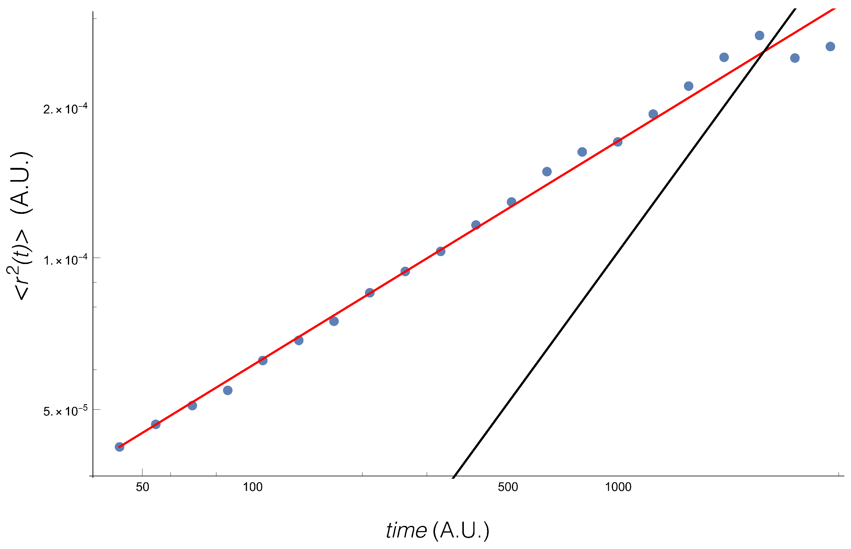
Following Reference [39], we computed measuring each day the second moment at different times.
The result (Figure 1) shows the well known fact that the diffusion is anomalous, with an exponent .
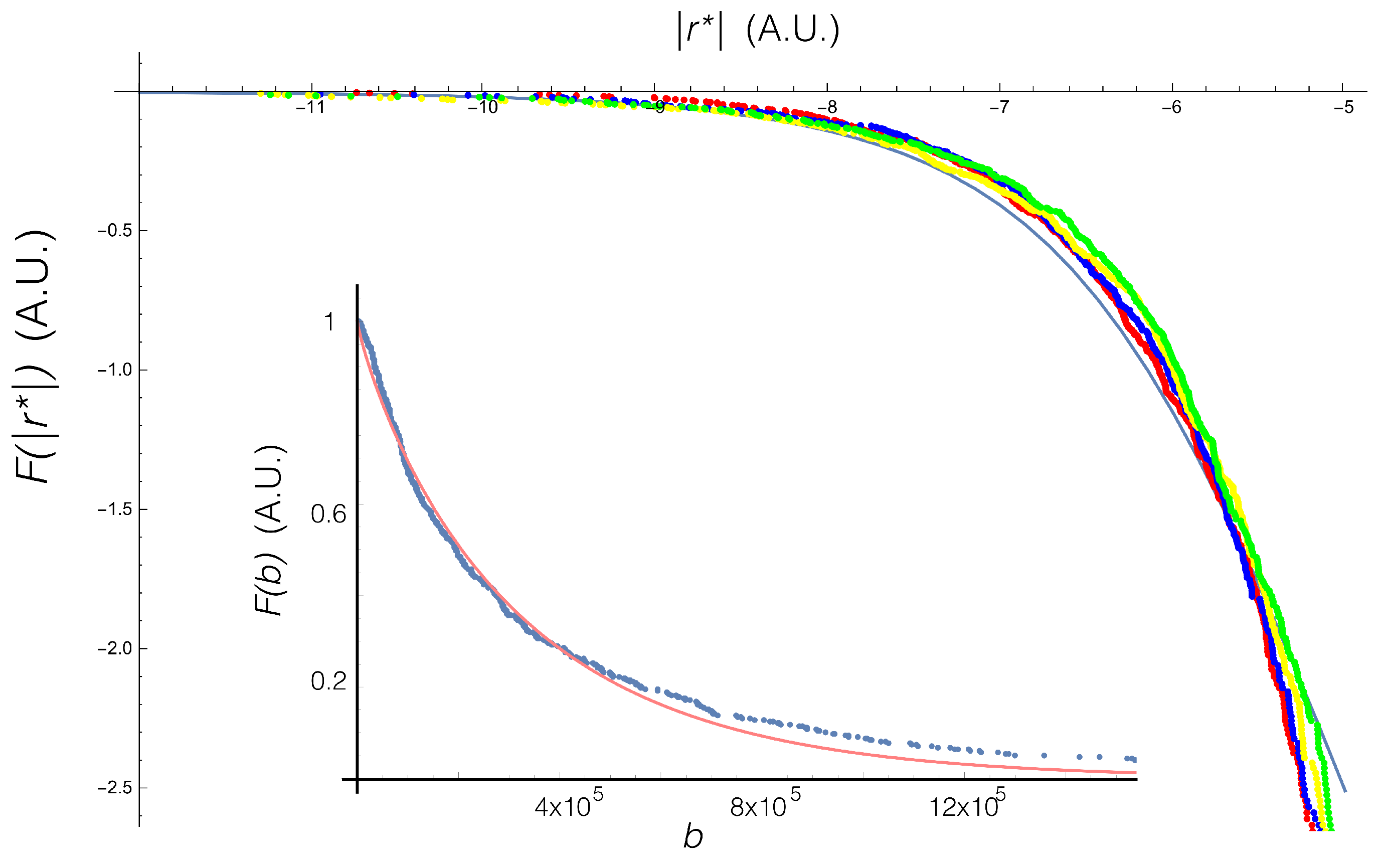
We then measured the different values of b, the inverse of the variance, for each day. We obtained the gamma distribution written in Equation (15) and performed the integration, Equation (13). Following these steps we found the analytic distribution Equation (22).
In Figure 2 we show the collapse of the complementary cumulative distribution F, where is defined (for a given ) as
and
The figure shows the empirical result for various times (different colors in the figure). The analytical result is also shown. We include an inset showing the complementary cumulative distribution for the parameter b.
6. Final Remarks
In the present work, we have shown that it is possible to obtain important behaviors, ubiquitous in many systems. First, we found that power laws are not only present in the distribution of variables that are relevant in the understanding of a physical problem, but also in the dynamical properties of them. We have also shown an analytical way to connect the microscopic characteristics of a single particle, with the microscopic characteristics of the full system. Among the main results obtained we find that anomalous behaviors appear in the financial time series when considering the price at time zero as a reference for the return. Another result is the possibility of obtaining the fat tail distribution when using the same approach. It is worth noting that the previous results also holds (for ) for a temporally homogeneous Gauss–Markov process, like the mentioned Ornstein–Uhlenbeck process. In this case the function to be marginalized is the ubiquitous Gaussian distribution.
Funding
This research received no external funding
Acknowledgments
Miguel A. Fuentes would like to thank H. Miguel for the fruitful discussions regarding memory effects in discrete dynamic processes.
Conflicts of Interest
The author declares no conflict of interest.
References
- Horbach, J.; Siboni, N.H.; Schnyder, S.K. Anomalous transport in heterogeneous media. Eur. Phys. J. Spec. Top. 2017, 226, 3113–3128. [Google Scholar] [CrossRef]
- La Porta, A.; Voth, G.A.; Crawford, A.M.; Alexander, J.; Bodenschatz, E. Fluid particle accelerations in fully developed turbulence. Nature 2001, 409, 1017–1019. [Google Scholar] [CrossRef] [PubMed] [Green Version]
- Bouchaud, J.P.; Potters, M. Theory of Financial Risk and Derivative Pricing: From Statistical Physics to Risk Management; Cambridge University Press: Cambridge, UK, 2003. [Google Scholar]
- Zhao, Z.D.; Yang, Z.; Zhang, Z.; Zhou, T.; Huang, Z.G.; Lai, Y.C. Emergence of scaling in human-interest dynamics. Sci. Rep. 2013, 3, 3472. [Google Scholar] [CrossRef] [PubMed] [Green Version]
- Brockmann, D.; Hufnagel, L.; Geisel, T. The scaling laws of human travel. Nature 2006, 439, 462–465. [Google Scholar] [CrossRef] [PubMed] [Green Version]
- Van Kampen, N.G. Stochastic Processes in Physics and Chemistry; Elsevier: New York, NY, USA, 1992; Volume 1. [Google Scholar]
- Borland, L. Microscopic dynamics of the nonlinear Fokker-Planck equation: A phenomenological model. Phys. Rev. E 1998, 57, 6634. [Google Scholar] [CrossRef]
- Ribeiro, M.S.; Casas, G.A.; Nobre, F.D. Multi–diffusive nonlinear Fokker–Planck equation. J. Phys. A Math. Theor. 2017, 50, 065001. [Google Scholar] [CrossRef]
- Hanel, R.; Thurner, S. When do generalized entropies apply? How phase space volume determines entropy. Europhys. Lett. 2011, 96, 50003. [Google Scholar] [CrossRef] [Green Version]
- Gell-Mann, M.; Tsallis, C. (Eds.) Nonextensive Entropy: Interdisciplinary Applications; Oxford University Press on Demand: Oxford, UK, 2004. [Google Scholar]
- Zhang, Y.; Dong, Z.; Wang, S.; Ji, G.; Yang, J. Preclinical diagnosis of magnetic resonance (MR) brain images via discrete wavelet packet transform with Tsallis entropy and generalized eigenvalue proximal support vector machine (GEPSVM). Entropy 2015, 17, 1795–1813. [Google Scholar] [CrossRef]
- Ibrahim, R.W.; Jalab, H.A. Existence of Ulam stability for iterative fractional differential equations based on fractional entropy. Entropy 2015, 17, 3172–3181. [Google Scholar] [CrossRef]
- Fuentes, M.A.; Cáceres, M.O. Computing the non-linear anomalous diffusion equation from first principles. Phys. Lett. A 2008, 372, 1236–1239. [Google Scholar] [CrossRef]
- Bachelier, L. Théorie de la Spéculation; Gauthier-Villars: Paris, France, 1900. (In French) [Google Scholar]
- Osborne, M.F. Brownian motion in the stock market. Oper. Res. 1959, 7, 145–173. [Google Scholar] [CrossRef]
- Mandelbrot, B.B. The variation of certain speculative prices. In Fractals and Scaling in Finance; Springer: New York, NY, USA, 1997; pp. 371–418. [Google Scholar]
- Fama, E.F. The behavior of stock-market prices. J. Bus. 1965, 38, 34–105. [Google Scholar] [CrossRef]
- Mantegna, R.N.; Stanley, H.E. Scaling behaviour in the dynamics of an economic index. Nature 1995, 376, 46–49. [Google Scholar] [CrossRef]
- Zhao, P.; Zhou, B.; Wang, J. Non-Gaussian Closed Form Solutions for Geometric Average Asian Options in the Framework of Non-Extensive Statistical Mechanics. Entropy 2018, 20, 71. [Google Scholar] [CrossRef]
- Gençay, R.; Gradojevic, N. The tale of two financial crises: An entropic perspective. Entropy 2017, 19, 244. [Google Scholar] [CrossRef]
- Tateishi, A.A.; Lenzi, E.K.; da Silva, L.R.; Ribeiro, H.V.; Picoli, S., Jr.; Mendes, R.S. Different diffusive regimes, generalized Langevin and diffusion equations. Phys. Rev. E 2012, 85, 011147. [Google Scholar] [CrossRef] [PubMed]
- Tirnakli, U.; Bykkili, F.; Demirhan, D. Some bounds upon the nonextensivity parameter using the approximate generalized distribution functions. Phys. Lett. A 1998, 245, 62–66. [Google Scholar] [CrossRef] [Green Version]
- Kusnezov, D.; Bulgac, A.; Do Dang, G. Quantum levy processes and fractional kinetics. Phys. Rev. Lett. 1999, 82, 1136. [Google Scholar] [CrossRef]
- Lutz, E. Anomalous diffusion through coupling to a fractal environment: Microscopic derivation of the “whip-back” effect. Europhys. Lett. 2001, 54, 293. [Google Scholar] [CrossRef]
- Leggett, A.J.; Chakravarty, S.D.A.F.M.G.A.; Dorsey, A.T.; Fisher, M.P.; Garg, A.; Zwerger, W. Dynamics of the dissipative two-state system. Rev. Mod. Phys. 1987, 59, 1. [Google Scholar] [CrossRef]
- Saichev, A.I.; Zaslavsky, G.M. Fractional kinetic equations: Solutions and applications. Chaos Interdiscip. J. Nonlinear Sci. 1997, 7, 753–764. [Google Scholar] [CrossRef] [PubMed]
- Samko, S.G.; Kilbas, A.A.; Marichev, O.I. Fractional Integrals and Derivatives: Theory and Applications; Gordon and Breach: Yverdon, Switzerland, 1993; p. 44. [Google Scholar]
- Slezak, J.; Metzler, R.; Magdziarz, M. Superstatistical generalised Langevin equation. New J. Phys. 2018, 20, 1–25. [Google Scholar] [CrossRef]
- Hilfer, R. Applications of Fractional Calculus in Physics; World Scientific Publishing: Singapore, 2000. [Google Scholar]
- Erdelyi, A. Higher Transcendental Functions; McGraw-Hill: New York, NY, USA, 1955; Volume 3. [Google Scholar]
- Gardiner, C.W. Handbook of Stochastic Methods; Springer: Berlin, Germany, 2005. [Google Scholar]
- Wang, K.G. Long-time-correlation effects and biased anomalous diffusion. Phys. Rev. A 1992, 45, 833. [Google Scholar] [CrossRef] [PubMed]
- Mandelbrot, B.B.; Van Ness, J.W. Fractional Brownian motions, fractional noises and applications. SIAM Rev. 1968, 10, 422–437. [Google Scholar] [CrossRef]
- Oldham, K.; Spanier, J. The Fractional Calculus Theory and Applications of Differentiation and Integration to Arbitrary Order; Elsevier: New York, NY, USA, 1974; Volume 111. [Google Scholar]
- Miller, K.S.; Ross, B. An Introduction to the Fractional Calculus and Fractional Differential Equations; John Wiley & Sons: Hoboken, NJ, USA, 1993. [Google Scholar]
- Atangana, A.; Gómez-Aguilar, J.F. Decolonisation of fractional calculus rules: Breaking commutativity and associativity to capture more natural phenomena. Eur. Phys. J. Plus 2018, 133, 1–22. [Google Scholar] [CrossRef]
- Atangana, A. Non validity of index law in fractional calculus: A fractional differential operator with Markovian and non-Markovian properties. Phys. A Stat. Mech. Appl. 2018, 505, 688–706. [Google Scholar] [CrossRef]
- Beck, C. Lagrangian acceleration statistics in turbulent flows. Europhys. Lett. 2003, 64, 151. [Google Scholar] [CrossRef]
- Gerig, A.; Vicente, J.; Fuentes, M.A. Model for non-Gaussian intraday stock returns. Phys. Rev. E 2009, 80, 065102. [Google Scholar] [CrossRef] [PubMed]
Figure 1.
Second moment of the return.The red line corresponds to the empirical fit , while the black line shows .
Figure 1.
Second moment of the return.The red line corresponds to the empirical fit , while the black line shows .

Figure 2.
Collapse of the empirical complementarycumulative distribution for time , 200, 1000 and 2000. The continuous blue line is the theoretical curve, after the marginalization Equation (13). Inset: Complementary cumulative distribution for b, and the fit to a gamma distribution.
Figure 2.
Collapse of the empirical complementarycumulative distribution for time , 200, 1000 and 2000. The continuous blue line is the theoretical curve, after the marginalization Equation (13). Inset: Complementary cumulative distribution for b, and the fit to a gamma distribution.

© 2018 by the author. Licensee MDPI, Basel, Switzerland. This article is an open access article distributed under the terms and conditions of the Creative Commons Attribution (CC BY) license (http://creativecommons.org/licenses/by/4.0/).
Share and Cite
MDPI and ACS Style
Fuentes, M.A. Non-Linear Diffusion and Power Law Properties of Heterogeneous Systems: Application to Financial Time Series. Entropy 2018, 20, 649. https://doi.org/10.3390/e20090649
AMA Style
Fuentes MA. Non-Linear Diffusion and Power Law Properties of Heterogeneous Systems: Application to Financial Time Series. Entropy. 2018; 20(9):649. https://doi.org/10.3390/e20090649
Chicago/Turabian StyleFuentes, Miguel A. 2018. "Non-Linear Diffusion and Power Law Properties of Heterogeneous Systems: Application to Financial Time Series" Entropy 20, no. 9: 649. https://doi.org/10.3390/e20090649
Note that from the first issue of 2016, this journal uses article numbers instead of page numbers. See further details here.