Article

An Ensemble Learning Approach Based on Diffusion Tensor Imaging Measures for Alzheimer’s Disease Classification

1
Innovation Lab, Exprivia S.p.A., Via A. Olivetti 11, I-70056 Molfetta, Italy
2
Department of Electrical and Information Engineering (DEI), Politecnico di Bari, Via E. Orabona 4, I-70125 Bari, Italy
*
Author to whom correspondence should be addressed.
These authors contributed equally to this work.
Electronics 2021, 10(3), 249; https://doi.org/10.3390/electronics10030249
Submission received: 30 December 2020 / Revised: 18 January 2021 / Accepted: 19 January 2021 / Published: 22 January 2021
(This article belongs to the Special Issue Computational Intelligence in Healthcare)

Abstract

:
Recent advances in neuroimaging techniques, such as diffusion tensor imaging (DTI), represent a crucial resource for structural brain analysis and allow the identification of alterations related to severe neurodegenerative disorders, such as Alzheimer’s disease (AD). At the same time, machine-learning-based computational tools for early diagnosis and decision support systems are adopted to uncover hidden patterns in data for phenotype stratification and to identify pathological scenarios. In this landscape, ensemble learning approaches, conceived to simulate human behavior in making decisions, are suitable methods in healthcare prediction tasks, generally improving classification performances. In this work, we propose a novel technique for the automatic discrimination between healthy controls and AD patients, using DTI measures as predicting features and a soft-voting ensemble approach for the classification. We show that this approach, efficiently combining single classifiers trained on specific groups of features, is able to improve classification performances with respect to the comprehensive approach of the concatenation of global features (with an increase of up to 9 % on average) and the use of individual groups of features (with a notable enhancement in sensitivity of up to 11 % ). Ultimately, the feature selection phase in similar classification tasks can take advantage of this kind of strategy, allowing one to exploit the information content of data and at the same time reducing the dimensionality of the feature space, and in turn the computational effort.

1. Introduction

Alzheimer’s disease (AD) is the most common type of neurodegenerative disorder causing dementia, generally characterized by loss of memory and a progressive decline of cognitive functions. AD affects millions of people worldwide, and according to the World Alzheimer’s report 2015 [1], people affected by dementia will reach 131.5 million in 2050. The in vivo diagnosis of AD is still a hard task because of the diversity of symptoms manifested by patients. In this context, a very challenging goal is the development of innovative computational-intelligence-based diagnostic tools that can support physicians and specialists in the early identification of the pathology and in therapeutic plan decisions. Advances in neuroimaging techniques have been fundamental for structural and functional brain analysis allowing the identification of AD-related brain alterations [2,3,4]. Due to the difficulty of integrating data on a large scale, machine learning methods (ML) allowing patient classification driven by large amounts of data are gaining increasing interest in recent years in the field of digital healthcare [5,6]. ML algorithms are a collection of computational and statistical models that can learn through experience and make predictions based on new data [7]. Machine learning approaches are able to uncover patterns in the data for differentiating diagnostic groups and identifying pathological scenarios [8,9]. Several recent studies have analyzed the potential of applying ML-based analytical frameworks to MRI data for the characterization and the automatic diagnosis of AD [10,11,12,13]. Indeed, the biological hypothesis that the cognitive decline due to AD is related to a connectivity disruption between brain regions caused by white matter degeneration (WM) has been widely investigated in literature [14,15]. In this context, diffusion tensor imaging (DTI) has emerged in the last fifteen years as a promising technique that measures the diffusion of water along WM fibers, providing information on their integrity [16]. The trajectory and the integrity of the main WM fiber bundles in the brain can be evaluated by tracing the highly anisotropic diffusion of water along axons [17]. Since DTI is a neuroimaging technique capable of characterizing white matter fiber trajectories and of highlighting microscopic WM lesions in these bundles, it can be exploited to uncover signs of connectivity impairment not detectable by means of standard anatomical MRI. Among the different measures that can be calculated from the diffusion tensor [17], fractional anisotropy (FA) and mean diffusivity (MD) have played major roles as AD biomarkers [18]. As a matter of fact, in a healthy axon water diffusion is highly anisotropic, because it is almost completely bound in one direction; consequently, large values of FA paired to small MD measures usually describe non-pathological scenarios. From this perspective, DTI allows to investigate microstructural disease-related changes complementary to the information on brain atrophy highlighted by anatomical MRI.
Recent applications of DTI techniques, together with ML algorithms for the classification of AD, use three possible methods for feature extraction: region of interest (ROI)-based, voxel-based and tractography-based approaches. In a ROI-based approach, the brain is parceled into regions of interest, and the mean of the DTI measures is then calculated for each ROI. The DTI scalar indexes averaged over each ROI are then used as features for feeding ML algorithms to classify AD subjects also at early stages of the disease and for investigating WM integrity alterations [19,20]. Several studies based on this approach have been conducted with multimodal analysis [21]. In tractography-based approaches, DTI fiber tracking algorithms together with a parcelation scheme are used to model the brain as a network and to study its connectivity through graph theory. Network measures turned out to be effective variables to characterize the connectivity alterations due to AD [22,23,24], and valid features from which to build classification models [25,26,27]. In voxel-based approaches, starting from fractional anisotropy maps and using the tract-based spatial statistics, a white matter “skeleton” is obtained, containing WM tracts common to all subjects. The diffusion maps of each subject are projected onto the average fractional anisotropy skeleton; hence, all diffusivity measures of the voxels belonging to that skeleton can be exploited for feeding classification algorithms and for performing voxel-wise statistical analyses aimed at localizing brain changes related to the onset and development of the pathology.
Machine learning methods for the identification of AD phenotypes are typically based on individual classifiers [28,29,30] or ensembles of different classifiers trained on the same set of features [25,31]. Ensemble learning is a ML approach—generally improving classification performances [32,33]—that integrates multiple classifiers fed with the same group of features or with several vectors of variables describing different representations of the same physical phenomenon [34]. Ensemble learning was conceived to simulate human behavior in making decisions, and for this reason it can be a suitable approach in the medical diagnosis context, where humans usually ask the opinions of various doctors to increase the reliability of a diagnosis.
In this paper, we propose a novel classification framework based on ensemble learning for the automatic discrimination between healthy controls (HC) and AD cases, relying on DTI measures as predicting variables. This kind of ensemble method is able to conveniently exploit the informative contents of individual maps, associated with specific aspects of microstructural fiber integrity, and to enhance the generalization ability, taking into account the peculiarities of different classifiers related to each set of features. Moreover, this methodology is aimed at enhancing computational efficiency, focusing in particular on combinations of single groups of variables instead of considering the usual approach of global feature concatenation. The paper is organized as follows. Section 2 introduces the diffusion tensor imaging (DTI) techniques able to investigate white matter fiber integrity through measurement of anisotropy of WM tracts and water diffusion along them. In Section 3 after a brief description of feature extraction procedures and classification models adopted in the present work, a learning experiment is detailed. Finally, Section 4 reports the results of the experiment and Section 5 discusses the main findings together with future research directions.

2. Diffusion Tensor Imaging

Diffusion, also known as Brownian motion, is the process of the random constant microscopic molecular motion caused by heat. In an anisotropic mean, like WM, diffusion is characterized by a tensor, called the effective diffusion tensor D eff , which fully describes the molecular mobility along the three spatial directions and the correlations between these directions. In the framework of MRI-based neuroimaging, diffusion tensor imaging (DTI) is a technique which evaluates the location, orientation and anisotropy of the brain’s WM tracts, providing the estimation of the diffusion tensor for each voxel of the 3D image.
From a geometric point of view, the diffusion tensor completely characterizes the shape of an ellipsoid by means of six variables describing the diffusion coefficient of water molecules at a specific time in each direction. In the case of isotropic diffusion, the diffusion coefficient is equal in every direction and the ellipsoid turns into a sphere. Instead, in the case of anisotropic diffusion the greater mean diffusion along the longest axis of the ellipsoid is described by an elongated ellipsoid. The tensor matrix is symmetric according to a property describing the antipodal symmetry of Brownian motion that is called “conjugate symmetry”. The diagonal terms of the diffusion tensor quantify the intensity of diffusivity in each of three orthogonal directions. The off-diagonal terms (vanishing in case of isotropy) indicate the magnitude of diffusion along one direction arising from a concentration gradient in an orthogonal direction.
Therefore, diffusion data are crucial in order to gain information on tissue microstructure and architecture for each voxel [16,17]. In particular, the three eigenvectors and the eigenvalues λ 1 , λ 2 and λ 3 of D eff describe the directions and lengths of the three diffusion ellipsoid axes, respectively, in descending order of magnitude. The largest (primary) eigenvector and the related eigenvalue λ 1 represent the direction and magnitude of greatest water diffusion, respectively. The primary eigenvector provides an important contribution to the fiber tractography algorithms, since it indicates the orientation of axonal fiber bundles. Eigenvalue λ 1 , called “longitudinal diffusivity” (LD), indicates the diffusion rate along the fibers’ orientation. Eigenvalues λ 2 and λ 3 , associated with second and third eigenvectors orthogonal to the primary one, represent the magnitude of diffusion in the plane transverse to the axonal bundles. The mean value,
R D = λ 2 + λ 3 2 ,
is called “radial diffusivity” (RD). The mean diffusivity (MD) indicates the mean displacement of molecules (average ellipsoid size) and describes the directionally averaged diffusivity of water within a voxel. It is defined as the mean of the three eigenvalues:
M D = λ 1 + λ 2 + λ 3 3
The fractional anisotropy (FA) measures the degree of directionality of intravoxel diffusivity, i.e., the fraction of the diffusion that is anisotropic:
F A = 1 2 λ 1 λ 2 2 + λ 2 λ 3 2 + λ 3 λ 1 2 λ 1 2 + λ 2 2 + λ 3 2
This measure basically represents a distance between the tensor ellipsoidal shape from a perfect sphere. Values of the fractional anisotropy range from zero, meaning an isotropic diffusion, to 1, in case of a linear diffusion occurring only along the primary eigenvector. When λ 1 λ 2 , λ 3 , the fractional anisotropy measure is close to 1, indicating a preferred direction of diffusion.

3. Materials and Methods

3.1. Data Collection

Real-world data have been gathered from the Alzheimer’s Disease Neuroimaging Initiative (ADNI) which has the primary goal of testing whether serial magnetic resonance imaging (MRI), positron emission tomography (PET), other biological markers, and clinical and neuropsychological assessments can be combined to measure the progression of mild cognitive impairment (MCI) and early Alzheimer’s disease (AD) (for up-to-date information, see www.adni-info.org) [35].
The dataset is made of diffusion-weighted scans from a cohort of 92 subjects of both genders, with age ranging from 55 to 90, from the ADNI-GO and ADNI-2 phases. According to their diagnoses, the subjects were grouped into 49 HC and 43 AD patients. Pre-processed FA, MD, RD and LD maps, available in ADNI databases, were randomly selected from baseline and follow-up study visits. It is worth mentioning that healthy subjects did not report symptoms of mild cognitive impairment, dementia, or depression; subjects with AD were those who met the NINCDS/ADRDA criteria for probable AD. The acquisition of diffusion-weighted scans was carried out through a 3-T GE Medical Systems scanner. In particular, for each subject 46 distinct images were collected articulated in 41 diffusion-weighted images ( b = 1000 s/mm 2 ) and 5 scans with negligible diffusion effects ( b 0 images).

3.2. Image Processing and Feature Extraction

The first step of the image processing is a double registration step. It consists of aligning the maps of all subjects so that the same microstructural areas of the anatomical regions correspond to the same voxels in the images. Then the maps are transformed into an existing standard space template image (in this case the MNI152 standard space [36] is used). After the registration, the voxels belonging to the white matter main fiber tracts are extracted from each map.
Following the acquisition of general diffusivity maps (including FA, MD, RD and LD), for each subject, all image processing steps were performed with FMRIB Software Library (FSL) [37], and in particular its diffusion toolkit FDT. In order to carefully align FA, MD, RD and LD maps to a group-wise space and to focus the analysis only on voxels that belong to the WM fiber bundles, a tract-based spatial statistics (TBSS) [38] standard procedure, included in FSL, was performed according to the following steps:
1.
Application of a nonlinear registration for the alignment of all fractional anisotropy maps to a common registration template: in the present analysis, we used the mean FMRIB58_FA standard target, available with the software, obtained as the average of 58 FA images in the MNI152 standard space. This step was performed for MD, RD and LD maps too.
2.
Affine transformation of the entire aligned dataset to a 1 × 1 × 1 mm 3 standard space: the aligned maps were transformed into the standard space template MNI152.
3.
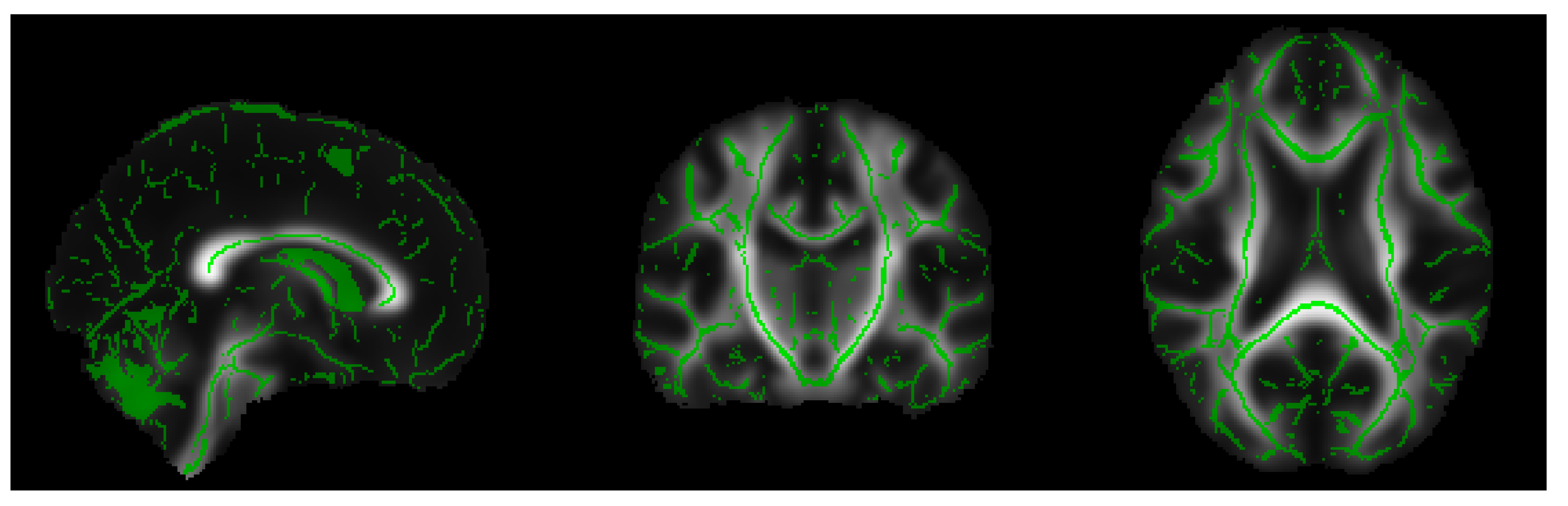
Extraction of the white matter skeleton: by averaging all the FA maps of the dataset, a mean FA image was obtained, and this result was used to create a mean FA skeleton of WM fiber tracts that were common to all subjects (see Figure 1). A threshold was applied to the mean FA skeleton in order to exclude gray matter and cerebrospinal fluid voxels, and the voxels of the zones characterized by greater inter-subject variability belonging to the outermost part of the cortex.
4.
Projection of all FA maps onto the mean FA skeleton: this allowed us to achieve an alignment among all subjects in the direction orthogonal to the fiber bundle orientation. The same elaboration steps were applied to RD, MD and LD maps.
The TBSS procedure generates, for each subject and for each diffusivity metric (FA, MD, RD, LD), approximately 9 × 10 4 voxels, belonging to the WM skeleton and representing the features of our classification task.

3.3. Classification Methods

Supervised learning methods are statistical learning techniques aimed to the classification of instances based on labeled training data. In the present paper, in order to build the ensemble approach, we investigate the most commonly used ML algorithms for medical classification tasks: support vector machine, random forest and multi-layer perceptron.
Support vector machine (SVM) [39] is a supervised learning algorithm based on the concept of an optimal hyper-plane that separates observations belonging to two different classes. In the case of a linear classification problem, given n data points belonging to two linearly separable sets in a p dimensional space, the task is to find a ( p 1 ) dimensional hyper-plane that can classify two classes with the largest margins, i.e., the largest distance to the boundary from the closest points in each set. In cases when data are not linearly separable, a possible solution is to map the original data onto a higher-dimensional feature space in order to favor a more effective separation. Support vector classifiers are then generalizations of the linear classifier approach to an “augmented” feature space with significantly high dimensionality (see left panel in Figure 2). Assuming that the transformed feature vectors are given by the function h ( x ) , the optimization problem can be conveniently recast as a quadratic programming problem using Lagrange multipliers in which the transformed vectors h ( x ) are involved in the form of scalar products. Thanks to this trick, it is not important to know the transformation, but only the type of the kernel function K ( x , x ) = h ( x ) , h ( x ) . Consequently, the configuration of a SVM classifier is completely characterized by the regularization parameter C and the choice of kernel function. In the present work, for the hyper-parameter tuning phase, the chosen functions are: (1) d degree polynomial: K ( x , x ) = ( 1 + x , x ) d ; (2) radial basis function (RBF): K ( x , x ) = exp ( γ | | x x | | 2 ) , where values of parameters d, γ , κ 1 and κ 2 span specific ranges.
Random forest (RF) is a supervised learning algorithm based on the construction of a collection of decision trees, known to be one of the best classifiers in terms of prediction accuracy and efficiency for high-dimensional datasets [40,41]. RF models operate by constructing a multitude of decision trees in the training phase and returning as a prediction the class predicted most frequently by each tree composing the forest, with the aim of reducing the variance of the final result. The RF training algorithm is based on the general technique of bootstrap aggregating to the trees under training. Let ( X , Y ) be the pair of training set X and target vector Y where X = { x 1 , , x n } and Y = y 1 , , y n . The strategy applies repeated (B times) extraction with the replacement of a random sample from X and a fit of the trees to this sample. In particular, for b = 1 , , B , the procedure is the following: (1) Random sampling with replacement of n observation from training set X obtaining the subsets ( X b , Y b ) . Generally, for a classification problem with p features, the cardinality of the subset is of order p in order to reduce the correlation between trees originated by bagging. (2) Training of the b-th tree f b on ( X b , Y b ) . (3) Out-of-sample prediction on unseen dataset x * is the response outcome obtained from the majority of the results generated by each single tree. The number of trees B in a forest is the free parameter of the model, usually set at an order of magnitude of at least 10 2 .
Multi-layer perceptron (MLP) [42] is a supervised learning algorithm using a feed-forward neural network technique. An MLP is composed of an input layer, one or more hidden layers of threshold logic units (TLUs) and an output layer. Each hidden layer is fully connected with the next one, and each TLU computes a weighted sum of its inputs then applies an activation function to provide a result that will be used as input for the next layer (see right panel in Figure 2). The activation function is in general nonlinear and is selected to be C 1 -differentiable. The learning process is based on the back-propagation algorithm that can be summarized as follows [43]: for each training instance, the algorithm generates a prediction and measures the performance (error). Consequently, each layer in reverse is analyzed in order to evaluate the contribution to the error from each connection; then edge weights are tuned in order to improve the performance. In this study, the hyper-parameter tuning phase of MLP is driven by the choice of an activation function and the number of hidden layers. Classification algorithms and performance metrics analyzed refer to the Python scikit-learn library [44].

3.4. Learning Experiment

Once the image processing and feature extraction procedure was completed, each subject was represented by different feature groups associated with diffusivity metrics (FA, MD, RD and LD) each with dimensions in the order of 10 5 . These groups can be used separately or combined in a single high-dimensional feature vector to feed a learning algorithm for the classification of patients with AD. The learning experiment proposed in the present work consists of comparing these two procedures with an ensemble learning approach in which each feature group is used to feed a classification algorithm and all the models are then combined through a voting scheme (see Figure 3). The idea is that different models trained independently can take into account different aspects of the data, and consequently a combination of algorithms can improve the predictions obtained with the single models in the ensemble. The ensemble configurations analyzed in this work are listed in Table 1.
The learning experiment consists of three steps.
1.
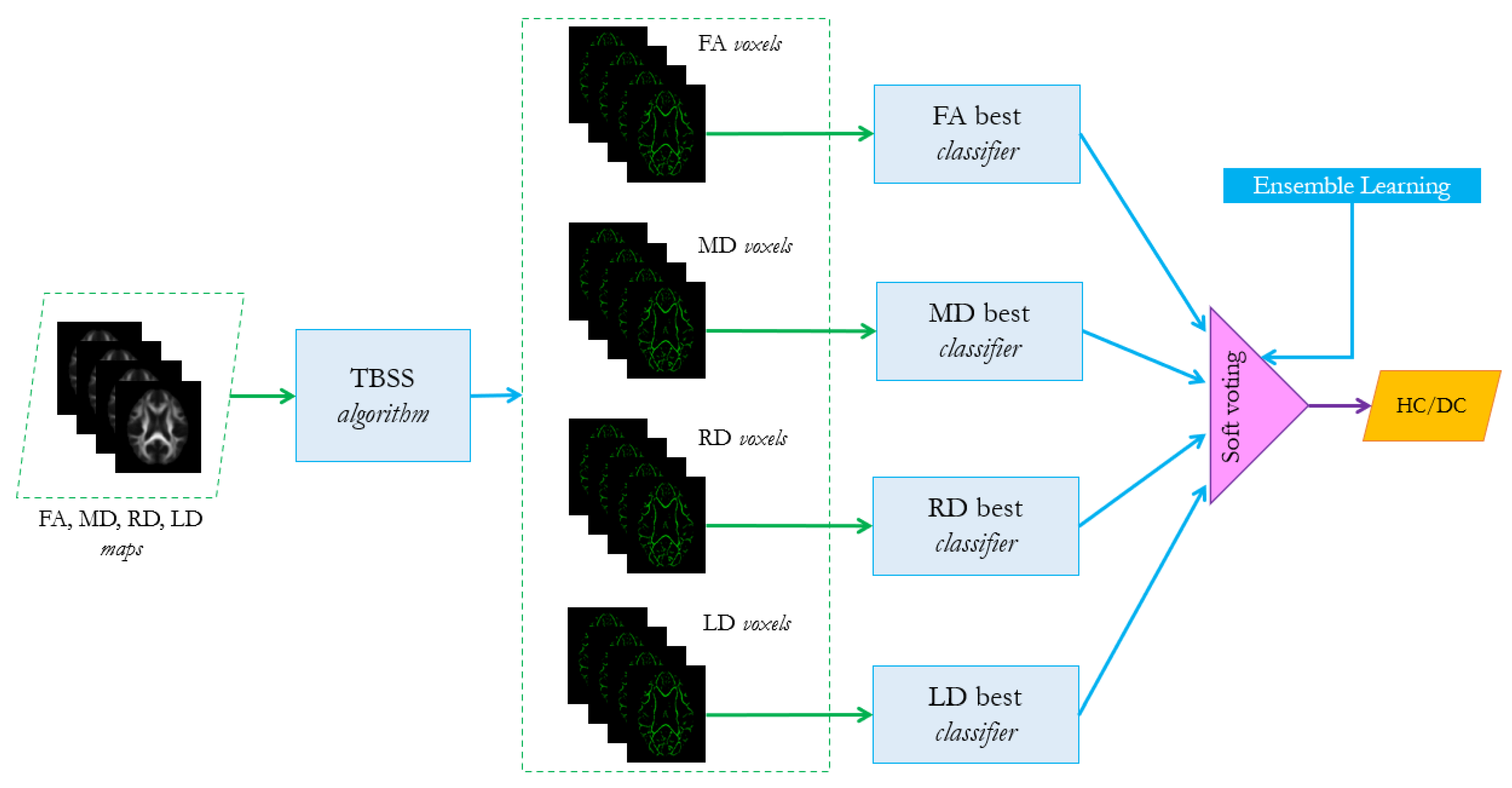
For each group of features in (FA, MD, RD, LD) and their combined feature vector, find the best associated classifier among the three algorithms SVM, RF and MLP, as described in Section 3.3. A 5-fold cross validation grid search procedure should be performed to tune the hyperparameters and evaluate the best performer for each configuration, as shown in Table 2.
For instance, for configuration 1-1 the model M F A is chosen among SVM b 1 - 1 , RF b 1 - 1 and MLP b 1 - 1 .
2.
For each possible configuration listed in Table 1, evaluate the performance of the ensemble learning algorithm, based on the combination of the best classifier selected in step 1. The voting scheme is a soft-voting procedure which is based on averaging the probability scores given by the individual classifiers according to the following equation:
y ^ = argmax i j = 1 n w j p i j
where y ^ is the ensemble predicted label, n is the number of classifiers, w j is the weight that can be assigned to the jth classifier (in the present analysis we consider uniform weights) and p i j is the probability score assigned to the ith class from the jth classifier. In the case of binary classification i 0 , 1 . The ensemble algorithm analyzed in the present work refers to the ensemble.VotingClassifier method of Python scikit-learn library [44]. The choice of this scheme is due to the fact that it is more flexible than the hard one, since it takes into account the classifiers’ uncertainty about the final decision, which is more informative than the simple binary prediction.
3.
Repeat steps 1 and 2 on a balanced dataset obtained from the original one (43 AD vs. 49 HC), removing 6 healthy controls using the instance hardness threshold method (IHT) of Smith et al. [45]. IHT is an under-sampling method for reducing class imbalance based on the removal of the “hard” instances (where instance hardness is the likelihood of being misclassified), while focusing on the majority class samples that overlap the minority class sample space. The balanced dataset is then composed of 43 diseased cases and 43 healthy controls.
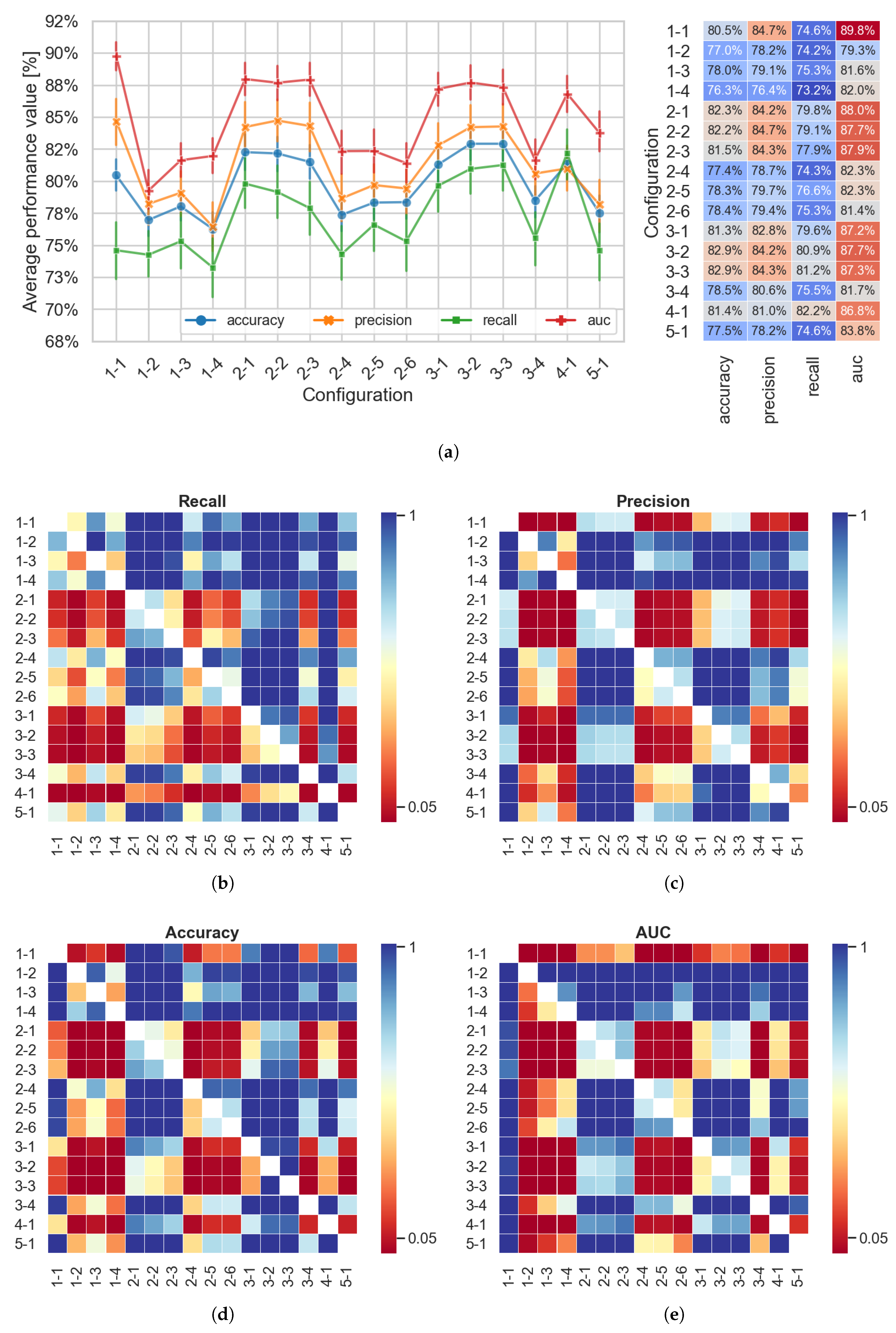
The classification performances in step 2 are evaluated through a 10-fold stratified cross-validation (CV) such that each fold is composed of approximately the same number of patients associated with each diagnostic group. This CV procedure was repeated ten times with different permutations of the training and test samples, in order to make the performance evaluation more robust and generalized. The metrics used for the performance assessment were accuracy, precision, recall and area under the ROC curve (AUC). For the comparison among ensemble combinations, statistically significant differences between the performances of classification configurations were assessed through non-parametric one-tailed Mann–Whitney U-test (MWU) [46]. Given F as the distribution function corresponding to population A and G as the distribution function corresponding to population B, MWU tested the null hypothesis H 0 : F ( t ) = G ( t ) , for every t (i.e., X and Y random variables have the same probability distribution) against the alternative hypothesis that Y is larger (or smaller) than X [47]. In order to address the problem of multiple comparison, p-values were corrected for multiple testing using the Benjamini–Hockberg (BH) procedure, summarized as follows: (1) Let H 1 , H 2 , , H N be the sequence of the null hypotheses to test with p 1 , p 2 , , p N as the associated p-values. (2) Rank p-values such that p ( 1 ) p ( 2 ) p ( 3 ) p ( N ) . (3) Given the level q * , find the largest k such that p ( k ) k · q * / N . (4) Reject all the null hypotheses H ( j ) with j = 1 , 2 , , k . The theorem of Benjamini–Hochberg states that the above procedure controls the false discovery rate with level q * [48].

4. Results

In this section, we outline the results of the experiment. Firstly, we discuss the effects of ensemble learning in terms of performances on the original imbalanced dataset; then we show the results for the balanced dataset obtained via instance hardness threshold method. Finally, we discuss the outcomes of nonparametric statistical tests carried out to compare the different configurations and to obtain an overview of the efficacy of the ensemble approach.
The results associated with the imbalanced case (49 HC, 43 AD) are reported in Figure 4. In panel (a), the performance average values are plotted as a function of the possible configurations. Each point in the plot represents the average over the 100 estimates of the performance metrics, obtained from the 10-times repeated, 10-fold stratified cross validations. The best configuration, according to the overall metrics, is the configuration 3-3 corresponding to the ensemble E ( M F A , M M D , M R D ) . In terms of accuracy, precision and AUC, the singleton E ( M F A ) outperformed the other individual configurations 1-2, 1-3, 1-4 and all other ensembles that did not contain fractional anisotropy as a feature group. On the other hand, in the case of recall, the ensemble strategy is crucial for enhancing the performances: almost all the ensemble configurations outperformed the single feature set configurations, and the best recall value was obtained for the most complex ensemble E ( M F A , M M D , M R D , M L D ) (configuration 4-1). The performance comparisons among all possible configurations were performed through a Mann–Whitney (MWU) test. The outcomes of MWU tests, for each performance measure, are reported in Panel (b-c-d-e). Each square of the heatmap represents the one-tailed MWU test between samples Y and X, where Y and X are given by 100 performance measures of the configurations on the y-axis and x-axis, respectively. The null hypothesis is that X and Y have the same probability distribution against the alternative hypothesis that Y is larger than X. The colors of heatmaps are related to the p-values of the test ranging from 0 (red) to 1 (blue). Levels shown in the maps refer to p-values corrected for multiple testing using the Benjamini–Hockberg procedure. Panel (b) shows that recall is generally enhanced by ensemble learning approaches and that ensemble configuration with n groups of features has higher sensitivity that those with n 1 groups. This behavior occurs in the other performance comparisons, with the exception that ensemble methods without fractional anisotropy are not affected by significant improvement. Finally, in order to test whether the balancing effects on the dataset can impact the performances of ensemble methods, due to the instance hardness threshold procedure, we performed the same comparisons of the imbalanced case on a fair ground of 43 diseased cases versus 43 healthy controls. The results associated with the balanced case are reported in Figure 5. As expected, we notice in panel (a) that the average performance values as a function of configurations are generally shifted upwards. Indeed, as shown by Wei et al. in [49] the use of balanced training data can provide the highest balanced performances in classifiers based on support vector machines, neural networks and decision trees. Conversely, the balancing procedure attenuates the ensemble effects in the enhancement of recall and predicting accuracy. From panels (b-c-d-e), the ensemble E ( M F A , M M D ) emerges as the best configuration over all performance measures, and all the methods that contain fractional anisotropy and mean diffusivity outperformed the E ( M FA , MD , RD , LD ) method that concatenates all features in a high-dimensional single vector.

5. Discussion and Conclusions

Computational systems aimed at the automatic classification of Alzheimer’s disease patients through voxel-based diffusivity measures have been widely investigated but mainly focused on the exploitation of individual learning methods. The authors of [18,50] used anisotropy and diffusivity voxels values of WM main tracts as features for HC/MCI discrimination with a single support vector machine, showing very high classification performances. However, as pointed out in [28], the key shortcoming of these approaches is given by a bias due to a non-nested feature selection method affecting the learning procedure. On the other hand, a recent study [30] based on an individual SVM classifier with Fisher score feature selection has reported valid performances focusing only on anisotropy measures of specific brain areas with well known AD-related connectivity abnormalities. Consequently, the idea of this work is to circumvent the problem of restricting the procedure to a single classifier or to an a priori selected group of features by exploiting all the information power of diffusion imaging techniques, through a computationally efficient learning strategy based on combinations of several feature groups and different classifiers. As a matter of fact, the simple concatenation of all feature groups (FA, MD, RD, LD) in a single high-dimensional vector would not be convenient in terms of time complexity and machinery efforts. Therefore, this approach addresses the problem of handling and selecting variables in the conditions where the feature dimensions are much larger than sample sizes typically available in medical classification tasks. In this framework, we presented a novel approach based on an ensemble learning strategy which combines classifiers that take into account different perspectives of the microstructural white matter integrity associated with each feature group. The work in [51] applied a similar ensemble methodology, feeding an a priori specified classifier with different tractography network measures describing specific aspects of brain connectivity.
We have investigated the validity of this ensemble learning procedure in the classification of HC vs. AD patients, in both cases of the original imbalanced dataset and a balanced dataset obtained by the instance hardness threshold under-sampling method. In particular, in the imbalanced case we found that all the ensemble combinations, including FA invariants, outperformed the singletons E ( M M D ) , E ( M R D ) and E ( M L D ) , and also the single vector containing all the feature groups. These results show the crucial contribution of fractional anisotropy in the correct classification of diseased subjects. In fact, fractional anisotropy, defined from diffusion tensor fitting as the degree of directionality of intravoxel diffusivity, has a behavior heavily related to variations in fiber density, axonal diameter and myelination in white matter in the presence of the onset of neurodegenerative diseases. According to Pierpaoli et al. [52], a hallmark of damage in white matter is the generalized loss of fiber tract integrity. Interestingly, further studies have shown that FA-associated voxel values have been able to uncover voxel microstructural alterations in the brains of AD patients at early stages too [18,28,53,54]. Moreover, while for AUC, accuracy and precision, the ensemble method did not significantly improve the performances of the single FA, the ensemble strategy was crucial for enhancing the recall of the classification framework. Furthermore, it is worth mentioning that, in terms of accuracy and sensitivity, the use of ensembles of classifiers associated with the diffusion measures not only turned out to be better than considering all measures concatenated in a single feature vector, but also provided higher performances as the combinations’ dimensions increased. In the balanced scenario, mean diffusivity emerged as the second most informative measure for pathology discrimination. This evidence is supported by the fact that MD represents the overall mean squared displacement of molecules in the non-collinear directions of free diffusion. Consequently, a variation of mean diffusivity is a signal of an increase in free water diffusion and in turn of a loss of anisotropy of molecular mobility [52]. In literature there is evidence supporting the hypothesis that the microstructural alterations in molecular diffusivity along white matter fiber bundles, described by MD, may be of higher predictive value compared to FA microstructural changes [55,56]. In the balanced case, the effects on the improvement of accuracy and recall of the ensemble procedure were attenuated. However, ensemble combinations that included FA and MD performed better than other variable sets considered individually and than the feature vector concatenating all groups together.
Based on results emerging in the present analysis, we can conclude that our ensemble classification framework, based on DTI features, is effective to improve HC/AD classification performances, and that ensembles including FA and MD are the best performing, confirming their role in the literature as most effective DTI measures for AD detection [57,58,59,60]. Moreover, although artificial data balancing attenuates the benefits of ensemble learning, the ensemble-based strategy generates significant improvements in the classification sensitivity and accuracy with respect to the general concatenation of all features into a high-dimensional vector. For this reason, the feature selection phase in similar classification tasks can take advantage of this kind of strategy, allowing one to exploit as much information as possible, but at the same time reducing the dimensionality of the feature space, and in turn the computational effort. Hence, the ensemble learning can be a promising approach to combining different types of features derived for DTI data, extending the application to DTI tractography network measures and diffusion voxel-based features.
Future advancements of the present work will consider firstly an extension of dataset size in order to ensure more robust procedures of algorithms calibration and validation. In this scenario, one would be enabled to analyze feature selection methods together with several families of classifiers in more extensive ensemble strategies. Indeed, the possibility of comparisons on a wider base between pairs of feature selectors and classifiers could lead to the identification of efficient methods for discriminating between diseased cases and healthy controls (for a thorough review of this kind of approach, see the large comparative study performed by Parmar et al. in [61]). Moreover, the availability of a larger number of observations would allow the application of state-of-the-art deep learning methods that could give important contributions in the uncovering of signatures and biomarkers of neurodegenerative disorders for highlighting hidden patterns. The key advantage of deep learning architectures with respect to standard learning approaches is given by the evidence that high values of classification performance can be optimally achieved without feature selection steps that are embedded in the process, yielding more computationally efficient frameworks (for an application of deep convolutional neural networks to MRI data, see the work of Basaia et al. in [62], and for a review of deep learning methods and applications in neuroimaging data in psychiatric and neurologica disorders, see [63]). Future investigations may also take into account not only diffusion-derived features, but also additional variables, such as clinical information, morphological measures and other features related to different image processing modalities and methodologies, such as functional and anatomical magnetic resonance imaging. As a matter of fact, a diversified plethora of biological information generated by different diagnostic modalities can provide not only a holistic view of the pathological condition, but can be exploited in the pre-clinical stage for the early detection of dementia precursors in presymptomatic conditions [64,65,66].

Author Contributions

Conceptualization, E.L.; methodology, E.L., A.P. and R.A.; software, E.L. and A.P.; validation, E.L., A.P., D.L., R.A. and F.V.; formal analysis, E.L. and R.A.; investigation, E.L., A.P., D.L. and R.A.; resources, E.L.; data curation, E.L.; writing—original draft preparation, E.L. and R.A.; writing—review and editing, E.L., A.P., D.L., R.A. and F.V.; visualization, E.L. and R.A.; supervision, R.A. and F.V. All authors have read and agreed to the published version of the manuscript.

Funding

This research was funded by Ministero dello Sviluppo Economico (MiSE) “Grandi Progetti R&S—PON 2014/2020 Agenda Digitale e Industria sostenibile”—BigImaging Project—Grant number F/080022/01-04/X35.

Data Availability Statement

Publicly available datasets were analyzed in this study. This data can be found here: www.adni-info.org.

Acknowledgments

Data collection and sharing for this project was funded by the Alzheimer’s Disease Neuroimaging Initiative (ADNI) (National Institutes of Health Grant U01 AG024904) and DOD ADNI (Department of Defense award number W81XWH-12-2-0012). ADNI is funded by the National Institute on Aging, the National Institute of Biomedical Imaging and Bioengineering, and through generous contributions from the following: AbbVie, Alzheimer’s Association; Alzheimer’s Drug Discovery Foundation; Araclon Biotech; BioClinica, Inc.; Biogen; Bristol-Myers Squibb Company; CereSpir, Inc.; Cogstate; Eisai Inc.; Elan Pharmaceuticals, Inc.; Eli Lilly and Company; EuroImmun; F. Hoffmann-La Roche Ltd and its affiliated company Genentech, Inc.; Fujirebio; GE Healthcare; IXICO Ltd.; Janssen Alzheimer Immunotherapy Research & Development, LLC.; Johnson and Johnson Pharmaceutical Research and Development LLC.; Lumosity; Lundbeck; Merck and Co., Inc.; Meso Scale Diagnostics, LLC.; NeuroRx Research; Neurotrack Technologies; Novartis Pharmaceuticals Corporation; Pfizer Inc.; Piramal Imaging; Servier; Takeda Pharmaceutical Company; and Transition Therapeutics. The Canadian Institutes of Health Research are providing funds to support ADNI clinical sites in Canada. Private sector contributions are facilitated by the Foundation for the National Institutes of Health (www.fnih.org). The grantee organization is the Northern California Institute for Research and Education, and the study is coordinated by the Alzheimer’s Therapeutic Research Institute at the University of Southern California. ADNI data are disseminated by the Laboratory for Neuro Imaging at the University of Southern California.

Conflicts of Interest

The authors declare no conflict of interest.

References

  1. Prince, M.J. World Alzheimer Report 2015: The Global Impact of Dementia: An Analysis of Prevalence, Incidence, Cost and Trends; Alzheimer’s Disease International: London, UK, 2015. [Google Scholar]
  2. Rombouts, S.A.; Barkhof, F.; Goekoop, R.; Stam, C.J.; Scheltens, P. Altered resting state networks in mild cognitive impairment and mild Alzheimer’s disease: An fMRI study. Hum. Brain Mapp. 2005, 26, 231–239. [Google Scholar] [CrossRef]
  3. Zhao, X.; Liu, Y.; Wang, X.; Liu, B.; Xi, Q.; Guo, Q.; Jiang, H.; Jiang, T.; Wang, P. Disrupted small-world brain networks in moderate Alzheimer’s disease: A resting-state FMRI study. PLoS ONE 2012, 7, e33540. [Google Scholar] [CrossRef] [Green Version]
  4. Lella, E.; Amoroso, N.; Lombardi, A.; Maggipinto, T.; Tangaro, S.; Bellotti, R.; Initiative, A.D.N. Communicability disruption in Alzheimer’s disease connectivity networks. J. Complex Netw. 2019, 7, 83–100. [Google Scholar] [CrossRef]
  5. Sidey-Gibbons, J.A.; Sidey-Gibbons, C.J. Machine learning in medicine: A practical introduction. BMC Med. Res. Methodol. 2019, 19, 64. [Google Scholar] [CrossRef] [PubMed] [Green Version]
  6. Al-Turjman, F.; Nawaz, M.H.; Ulusar, U.D. Intelligence in the Internet of medical things era: A systematic review of current and future trends. Comput. Commun. 2020, 150, 644–660. [Google Scholar] [CrossRef]
  7. Jordan, M.I.; Mitchell, T.M. Machine learning: Trends, perspectives, and prospects. Science 2015, 349, 255–260. [Google Scholar] [CrossRef]
  8. Casalino, G.; Castellano, G.; Consiglio, A.; Liguori, M.; Nuzziello, N.; Primiceri, D. A Predictive Model for MicroRNA Expressions in Pediatric Multiple Sclerosis Detection. In International Conference on Modeling Decisions for Artificial Intelligence; Springer: Berlin/Heidelberg, Germany, 2019; pp. 177–188. [Google Scholar]
  9. Angelillo, M.T.; Balducci, F.; Impedovo, D.; Pirlo, G.; Vessio, G. Attentional pattern classification for automatic dementia detection. IEEE Access 2019, 7, 57706–57716. [Google Scholar] [CrossRef]
  10. Dyrba, M.; Ewers, M.; Wegrzyn, M.; Kilimann, I.; Plant, C.; Oswald, A.; Meindl, T.; Pievani, M.; Bokde, A.L.; Fellgiebel, A.; et al. Robust automated detection of microstructural white matter degeneration in Alzheimer’s disease using machine learning classification of multicenter DTI data. PLoS ONE 2013, 8, e64925. [Google Scholar] [CrossRef]
  11. Lella, E.; Amoroso, N.; Bellotti, R.; Diacono, D.; La Rocca, M.; Maggipinto, T.; Monaco, A.; Tangaro, S. Machine learning for the assessment of Alzheimer’s disease through DTI. SPIE Proc. 2017, 10396, 1039619. Available online: https://www.spiedigitallibrary.org/conference-proceedings-of-spie/10396/2293188/Front-Matter-Volume-10396/10.1117/12.2293188.full?SSO=1 (accessed on 21 January 2021).
  12. Lian, C.; Liu, M.; Zhang, J.; Shen, D. Hierarchical fully convolutional network for joint atrophy localization and Alzheimer’s Disease diagnosis using structural MRI. IEEE Trans. Pattern Anal. Mach. Intell. 2018, 42, 880–893. [Google Scholar] [CrossRef]
  13. Wee, C.Y.; Yap, P.T.; Li, W.; Denny, K.; Browndyke, J.N.; Potter, G.G.; Welsh-Bohmer, K.A.; Wang, L.; Shen, D. Enriched white matter connectivity networks for accurate identification of MCI patients. Neuroimage 2011, 54, 1812–1822. [Google Scholar] [CrossRef] [PubMed] [Green Version]
  14. Rose, S.E.; Chen, F.; Chalk, J.B.; Zelaya, F.O.; Strugnell, W.E.; Benson, M.; Semple, J.; Doddrell, D.M. Loss of connectivity in Alzheimer’s disease: An evaluation of white matter tract integrity with colour coded MR diffusion tensor imaging. J. Neurol. Neurosurg. Psychiatry 2000, 69, 528–530. [Google Scholar] [CrossRef] [PubMed] [Green Version]
  15. Head, D.; Buckner, R.L.; Shimony, J.S.; Williams, L.E.; Akbudak, E.; Conturo, T.E.; McAvoy, M.; Morris, J.C.; Snyder, A.Z. Differential vulnerability of anterior white matter in nondemented aging with minimal acceleration in dementia of the Alzheimer type: Evidence from diffusion tensor imaging. Cereb. Cortex 2004, 14, 410–423. [Google Scholar] [CrossRef] [PubMed] [Green Version]
  16. Basser, P.J.; Mattiello, J.; LeBihan, D. MR diffusion tensor spectroscopy and imaging. Biophys. J. 1994, 66, 259–267. [Google Scholar] [CrossRef] [Green Version]
  17. Le Bihan, D.; Mangin, J.F.; Poupon, C.; Clark, C.A.; Pappata, S.; Molko, N.; Chabriat, H. Diffusion tensor imaging: Concepts and applications. J. Magn. Reson. Imaging 2001, 13, 534–546. [Google Scholar] [CrossRef] [PubMed]
  18. O’Dwyer, L.; Lamberton, F.; Bokde, A.L.; Ewers, M.; Faluyi, Y.O.; Tanner, C.; Mazoyer, B.; O’Neill, D.; Bartley, M.; Collins, D.R.; et al. Using support vector machines with multiple indices of diffusion for automated classification of mild cognitive impairment. PLoS ONE 2012, 7, e32441. [Google Scholar] [CrossRef] [PubMed]
  19. Mesrob, L.; Sarazin, M.; Hahn-Barma, V.; Souza, L.C.D.; Dubois, B.; Gallinari, P.; Kinkingnéhun, S. DTI and structural MRI classification in Alzheimer’s disease. Adv. Mol. Imaging 2012, 2, 12–20. [Google Scholar] [CrossRef] [Green Version]
  20. Dyrba, M.; Barkhof, F.; Fellgiebel, A.; Filippi, M.; Hausner, L.; Hauenstein, K.; Kirste, T.; Teipel, S.J. Predicting Prodromal Alzheimer’s Disease in Subjects with Mild Cognitive Impairment Using Machine Learning Classification of Multimodal Multicenter Diffusion-Tensor and Magnetic Resonance Imaging Data. J. Neuroimaging 2015, 25, 738–747. [Google Scholar] [CrossRef]
  21. Dyrba, M.; Grothe, M.; Kirste, T.; Teipel, S.J. Multimodal analysis of functional and structural disconnection in Alzheimer’s disease using multiple kernel SVM. Hum. Brain Mapp. 2015, 36, 2118–2131. [Google Scholar] [CrossRef]
  22. Lella, E.; Estrada, E. Communicability distance reveals hidden patterns of Alzheimer’s disease. Netw. Neurosci. 2020, 4, 1–23. [Google Scholar] [CrossRef]
  23. Rasero, J.; Alonso-Montes, C.; Diez, I.; Olabarrieta-Landa, L.; Remaki, L.; Escudero, I.; Mateos, B.; Bonifazi, P.; Fernandez, M.; Arango-Lasprilla, J.C.; et al. Group-level progressive alterations in brain connectivity patterns revealed by diffusion-tensor brain networks across severity stages in Alzheimer’s disease. Front. Aging Neurosci. 2017, 9, 215. [Google Scholar] [CrossRef] [PubMed] [Green Version]
  24. Daianu, M.; Jahanshad, N.; Nir, T.M.; Toga, A.W.; Jack, C.R., Jr.; Weiner, M.W.; Thompson, P.M. Breakdown of brain connectivity between normal aging and Alzheimer’s disease: A structural k-core network analysis. Brain Connect. 2013, 3, 407–422. [Google Scholar] [CrossRef] [PubMed] [Green Version]
  25. Ebadi, A.; Dalboni da Rocha, J.L.; Nagaraju, D.B.; Tovar-Moll, F.; Bramati, I.; Coutinho, G.; Sitaram, R.; Rashidi, P. Ensemble classification of Alzheimer’s disease and mild cognitive impairment based on complex graph measures from diffusion tensor images. Front. Neurosci. 2017, 11, 56. [Google Scholar] [CrossRef] [PubMed] [Green Version]
  26. Prasad, G.; Joshi, S.H.; Nir, T.M.; Toga, A.W.; Thompson, P.M.; Alzheimer’s Disease Neuroimaging Initiative (ADNI). Brain connectivity and novel network measures for Alzheimer’s disease classification. Neurobiol. Aging 2015, 36, S121–S131. [Google Scholar] [CrossRef] [PubMed] [Green Version]
  27. Lella, E.; Lombardi, A.; Amoroso, N.; Diacono, D.; Maggipinto, T.; Monaco, A.; Bellotti, R.; Tangaro, S. Machine learning and dwi brain communicability networks for alzheimer’s disease detection. Appl. Sci. 2020, 10, 934. [Google Scholar] [CrossRef] [Green Version]
  28. Maggipinto, T.; Bellotti, R.; Amoroso, N.; Diacono, D.; Donvito, G.; Lella, E.; Monaco, A.; Scelsi, M.A.; Tangaro, S. DTI measurements for Alzheimer’s classification. Phys. Med. Biol. 2017, 62, 2361. [Google Scholar] [CrossRef]
  29. Dou, X.; Yao, H.; Feng, F.; Wang, P.; Zhou, B.; Jin, D.; Yang, Z.; Li, J.; Zhao, C.; Wang, L.; et al. Characterizing white matter connectivity in Alzheimer’s disease and mild cognitive impairment: An automated fiber quantification analysis with two independent datasets. Cortex 2020, 129, 390–405. [Google Scholar] [CrossRef]
  30. Da Rocha, J.L.D.; Bramati, I.; Coutinho, G.; Moll, F.T.; Sitaram, R. Fractional Anisotropy changes in parahippocampal cingulum due to Alzheimer’s Disease. Sci. Rep. 2020, 10, 1–8. [Google Scholar]
  31. Islam, J.; Zhang, Y. Brain MRI analysis for Alzheimer’s disease diagnosis using an ensemble system of deep convolutional neural networks. Brain Inform. 2018, 5, 2. [Google Scholar] [CrossRef]
  32. Suk, H.I.; Lee, S.W.; Shen, D.; Alzheimer’s Disease Neuroimaging Initiative. Deep ensemble learning of sparse regression models for brain disease diagnosis. Med. Image Anal. 2017, 37, 101–113. [Google Scholar] [CrossRef] [Green Version]
  33. Zheng, X.; Shi, J.; Zhang, Q.; Ying, S.; Li, Y. Improving MRI-based diagnosis of Alzheimer’s disease via an ensemble privileged information learning algorithm. In Proceedings of the 2017 IEEE 14th International Symposium on Biomedical Imaging (ISBI 2017), Melbourne, Australia, 18–21 April 2017; pp. 456–459. [Google Scholar]
  34. Rokach, L. Ensemble-based classifiers. Artif. Intell. Rev. 2010, 33, 1–39. [Google Scholar] [CrossRef]
  35. Petersen, R.C.; Aisen, P.; Beckett, L.A.; Donohue, M.; Gamst, A.; Harvey, D.J.; Jack, C.; Jagust, W.; Shaw, L.; Toga, A.; et al. Alzheimer’s disease neuroimaging initiative (ADNI): Clinical characterization. Neurology 2010, 74, 201–209. [Google Scholar] [CrossRef] [PubMed] [Green Version]
  36. Maintz, J.A.; Viergever, M.A. A survey of medical image registration. Med. Image Anal. 1998, 2, 1–36. [Google Scholar] [CrossRef]
  37. Jenkinson, M.; Beckmann, C.F.; Behrens, T.E.; Woolrich, M.W.; Smith, S.M. FSL. Neuroimage 2012, 62, 782–790. [Google Scholar] [CrossRef] [Green Version]
  38. Smith, S.M.; Jenkinson, M.; Johansen-Berg, H.; Rueckert, D.; Nichols, T.E.; Mackay, C.E.; Watkins, K.E.; Ciccarelli, O.; Cader, M.Z.; Matthews, P.M.; et al. Tract-based spatial statistics: Voxelwise analysis of multi-subject diffusion data. Neuroimage 2006, 31, 1487–1505. [Google Scholar] [CrossRef]
  39. Cortes, C.; Vapnik, V. Support-vector networks. Mach. Learn. 1995, 20, 273–297. [Google Scholar] [CrossRef]
  40. Ho, T.K. The random subspace method for constructing decision forests. IEEE Trans. Pattern Anal. Mach. Intell. 1998, 20, 832–844. [Google Scholar] [CrossRef] [Green Version]
  41. Breiman, L. Random Forests. Mach. Learn. 2001, 45, 5–32. [Google Scholar] [CrossRef] [Green Version]
  42. Murtagh, F. Multilayer perceptrons for classification and regression. Neurocomputing 1991, 2, 183–197. [Google Scholar] [CrossRef]
  43. Géron, A. Hands-On Machine Learning with Scikit-Learn, Keras, and TensorFlow: Concepts, Tools, and Techniques to Build Intelligent Systems; O’Reilly Media: Sebastopol, CA, USA, 2019. [Google Scholar]
  44. Pedregosa, F.; Varoquaux, G.; Gramfort, A.; Michel, V.; Thirion, B.; Grisel, O.; Blondel, M.; Prettenhofer, P.; Weiss, R.; Dubourg, V.; et al. Scikit-learn: Machine Learning in Python. J. Mach. Learn. Res. 2011, 12, 2825–2830. [Google Scholar]
  45. Smith, M.R.; Martinez, T.; Giraud-Carrier, C. An instance level analysis of data complexity. Mach. Learn. 2014, 95, 225–256. [Google Scholar] [CrossRef] [Green Version]
  46. Mann, H.B.; Whitney, D.R. On a test of whether one of two random variables is stochastically larger than the other. Ann. Math. Stat. 1947, 18, 50–60. [Google Scholar] [CrossRef]
  47. Hollander, M. Nonparametric Statistical Methods; John Wiley & Sons, Inc.: Hoboken, NJ, USA, 2013. [Google Scholar]
  48. Benjamini, Y.; Hochberg, Y. Controlling the False Discovery Rate: A Practical and Powerful Approach to Multiple Testing. J. R. Stat. Soc. Ser. B Methodol. 1995, 57, 289–300. [Google Scholar] [CrossRef]
  49. Wei, Q.; Dunbrack, R.L., Jr. The role of balanced training and testing data sets for binary classifiers in bioinformatics. PLoS ONE 2013, 8, e67863. [Google Scholar] [CrossRef] [PubMed] [Green Version]
  50. Haller, S.; Nguyen, D.; Rodriguez, C.; Emch, J.; Gold, G.; Bartsch, A.; Lovblad, K.O.; Giannakopoulos, P. Individual prediction of cognitive decline in mild cognitive impairment using support vector machine-based analysis of diffusion tensor imaging data. J. Alzheimer’s Dis. 2010, 22, 315–327. [Google Scholar] [CrossRef]
  51. Lella, E.; Vessio, G. Ensembling complex network ‘perspectives’ for mild cognitive impairment detection with artificial neural networks. Pattern Recognit. Lett. 2020, 136, 168–174. [Google Scholar] [CrossRef]
  52. Pierpaoli, C.; Jezzard, P.; Basser, P.J.; Barnett, A.; Di Chiro, G. Diffusion tensor MR imaging of the human brain. Radiology 1996, 201, 637–648. [Google Scholar] [CrossRef]
  53. Schouten, T.M.; Koini, M.; de Vos, F.; Seiler, S.; de Rooij, M.; Lechner, A.; Schmidt, R.; van den Heuvel, M.; van der Grond, J.; Rombouts, S.A. Individual classification of Alzheimer’s disease with diffusion magnetic resonance imaging. Neuroimage 2017, 152, 476–481. [Google Scholar] [CrossRef] [Green Version]
  54. Patil, R.B.; Ramakrishnan, S. Analysis of sub-anatomic diffusion tensor imaging indices in white matter regions of Alzheimer with MMSE score. Comput. Methods Programs Biomed. 2014, 117, 13–19. [Google Scholar] [CrossRef]
  55. Douaud, G.; Menke, R.A.; Gass, A.; Monsch, A.U.; Rao, A.; Whitcher, B.; Zamboni, G.; Matthews, P.M.; Sollberger, M.; Smith, S. Brain microstructure reveals early abnormalities more than two years prior to clinical progression from mild cognitive impairment to Alzheimer’s disease. J. Neurosci. 2013, 33, 2147–2155. [Google Scholar] [CrossRef] [Green Version]
  56. Nir, T.M.; Villalon-Reina, J.E.; Prasad, G.; Jahanshad, N.; Joshi, S.H.; Toga, A.W.; Bernstein, M.A.; Jack, C.R., Jr.; Weiner, M.W.; Thompson, P.M.; et al. Diffusion weighted imaging-based maximum density path analysis and classification of Alzheimer’s disease. Neurobiol. Aging 2015, 36, S132–S140. [Google Scholar] [CrossRef] [Green Version]
  57. Billeci, L.; Badolato, A.; Bachi, L.; Tonacci, A. Machine Learning for the Classification of Alzheimer’s Disease and Its Prodromal Stage Using Brain Diffusion Tensor Imaging Data: A Systematic Review. Processes 2020, 8, 1071. [Google Scholar] [CrossRef]
  58. Tu, M.C.; Lo, C.P.; Huang, C.F.; Hsu, Y.H.; Huang, W.H.; Deng, J.F.; Lee, Y.C. Effectiveness of diffusion tensor imaging in differentiating early-stage subcortical ischemic vascular disease, Alzheimer’s disease and normal ageing. PLoS ONE 2017, 12, e0175143. [Google Scholar] [CrossRef] [PubMed]
  59. Shao, J.; Myers, N.; Yang, Q.; Feng, J.; Plant, C.; Böhm, C.; Förstl, H.; Kurz, A.; Zimmer, C.; Meng, C.; et al. Prediction of Alzheimer’s disease using individual structural connectivity networks. Neurobiol. Aging 2012, 33, 2756–2765. [Google Scholar] [CrossRef] [Green Version]
  60. Graña, M.; Termenon, M.; Savio, A.; Gonzalez-Pinto, A.; Echeveste, J.; Pérez, J.; Besga, A. Computer aided diagnosis system for Alzheimer disease using brain diffusion tensor imaging features selected by Pearson’s correlation. Neurosci. Lett. 2011, 502, 225–229. [Google Scholar] [CrossRef] [PubMed]
  61. Parmar, C.; Grossmann, P.; Bussink, J.; Lambin, P.; Aerts, H.J. Machine learning methods for quantitative radiomic biomarkers. Sci. Rep. 2015, 5, 13087. [Google Scholar] [CrossRef]
  62. Basaia, S.; Agosta, F.; Wagner, L.; Canu, E.; Magnani, G.; Santangelo, R.; Filippi, M.; Alzheimer’s Disease Neuroimaging Initiative. Automated classification of Alzheimer’s disease and mild cognitive impairment using a single MRI and deep neural networks. NeuroImage Clin. 2019, 21, 101645. [Google Scholar] [CrossRef]
  63. Vieira, S.; Pinaya, W.H.; Mechelli, A. Using deep learning to investigate the neuroimaging correlates of psychiatric and neurological disorders: Methods and applications. Neurosci. Biobehav. Rev. 2017, 74, 58–75. [Google Scholar] [CrossRef] [Green Version]
  64. Alberdi, A.; Aztiria, A.; Basarab, A. On the early diagnosis of Alzheimer’s Disease from multimodal signals: A survey. Artif. Intell. Med. 2016, 71, 1–29. [Google Scholar] [CrossRef] [Green Version]
  65. Chételat, G. Multimodal neuroimaging in Alzheimer’s disease: Early diagnosis, physiopathological mechanisms, and impact of lifestyle. J. Alzheimer’s Dis. 2018, 64, S199–S211. [Google Scholar] [CrossRef]
  66. Ten Kate, M.; Redolfi, A.; Peira, E.; Bos, I.; Vos, S.J.; Vandenberghe, R.; Gabel, S.; Schaeverbeke, J.; Scheltens, P.; Blin, O.; et al. MRI predictors of amyloid pathology: Results from the EMIF-AD Multimodal Biomarker Discovery study. Alzheimer’s Res. Ther. 2018, 10, 100. [Google Scholar] [CrossRef] [PubMed]
Figure 1. Coronal, sagittal and axial views of the brain obtained in the FSLeyes image viewer: the mean fractional anisotropy (FA) skeleton (green) is overlaid with the mean FA map. For the following analysis all maps were projected onto the white matter skeleton.
Electronics 10 00249 g001
Figure 2. (a) Cartoon picture of a SVM classifier with nonlinear kernel: dots of different colors represent instances of two different classes; dotted lines represent the decision boundaries. (b) Example of a multi-layer perceptron with two hidden layers.
Electronics 10 00249 g002
Figure 3. Classification framework based on ensemble learning with a soft-voting strategy.
Electronics 10 00249 g003
Figure 4. The case of an imbalanced dataset. (a) Average performance values for each configuration. (be) Heatmaps of Mann–Whitney tests. Each square represents the p-value outcome of a one-tail Mann–Whitney test between a configuration on the y-axis and the other on the x-axis. Each p-value in the heatmap was corrected for multiple tests using the Benjamini–Hochberg procedure.
Electronics 10 00249 g004
Figure 5. The case of a balanced dataset. (a) Average performance values for each configuration. (be) Heatmaps of Mann–Whitney tests. Each square represents the p-value outcome of a one-tail Mann–Whitney test between a configuration on the y-axis and the other on the x-axis. Each p-value in a heatmap has been corrected for multiple tests using the Benjamini–Hochberg procedure.
Electronics 10 00249 g005
Table 1. List of all ensemble configurations.
LabelConfigurationLabelConfiguration
1-1 E ( M FA ) 2-5 E ( M LD , M RD )
1-2 E ( M MD ) 2-6 E ( M MD , M RD )
1-3 E ( M RD ) 3-1 E ( M FA , M LD , M MD )
1-4 E ( M LD ) 3-2 E ( M FA , M LD , M RD )
2-1 E ( M FA , M LD ) 3-3 E ( M FA , M MD , M RD )
2-2 E ( M FA , M MD ) 3-4 E ( M LD , M MD , M RD )
2-3 E ( M FA , M RD ) 4-1 E ( M FA , M MD , M RD , M LD )
2-4 E ( M LD , M MD ) 5-1 E ( M FA , MD , RD , LD )
Mi is the best classification method associated with the i-th feature group and E (M1, M2, …, Mj) is the ensemble learning method based on the combination of best classifiers M1, M2, …, Mj. The ensemble of a singleton corresponds to the best classifier, i.e., E (Mi) ≡ Mi. Finally, configuration 5-1 refers to the best classifier trained on a single high-dimensional vector concatenating all feature groups.
Table 2. Best model selection procedure.
1-11-21-31-45-1
5-fold SVM bestSVM b 1 - 1 SVM b 1 - 2 SVM b 1 - 3 SVM b 1 - 4 SVM b 5 - 1
5-fold RF bestRF b 1 - 1 RF b 1 - 2 RF b 1 - 3 RF b 1 - 4 RF b 5 - 1
5-fold MLP bestMLP b 1 - 1 MLP b 1 - 2 MLP b 1 - 3 MLP b 1 - 4 MLP b 5 - 1
Best Classifier M FA M MD M RD M LD M 5 - 1
Publisher’s Note: MDPI stays neutral with regard to jurisdictional claims in published maps and institutional affiliations.

