Article

Study of Quantized Hardware Deep Neural Networks Based on Resistive Switching Devices, Conventional versus Convolutional Approaches

by
Rocío Romero-Zaliz
1,
Eduardo Pérez
2,
Francisco Jiménez-Molinos
3,
Christian Wenger
2,4 and
Juan B. Roldán
3,*
1
Andalusian Research Institute on Data Science and Computational Intelligence (DaSCI), University of Granada, 18071 Granada, Spain
2
IHP-Leibniz-Institut für Innovative Mikroelektronik, 15236 Frankfurt, Germany
3
Departamento de Electrónica y Tecnología de Computadores, Universidad de Granada, 18071 Granada, Spain
4
Institute of Physics, Brandenburg University of Technology Cottbus-Senftenberg (BTU), 03046 Cottbus, Germany
*
Author to whom correspondence should be addressed.
Electronics 2021, 10(3), 346; https://doi.org/10.3390/electronics10030346
Submission received: 7 January 2021 / Revised: 22 January 2021 / Accepted: 26 January 2021 / Published: 1 February 2021

Abstract

:
A comprehensive analysis of two types of artificial neural networks (ANN) is performed to assess the influence of quantization on the synaptic weights. Conventional multilayer-perceptron (MLP) and convolutional neural networks (CNN) have been considered by changing their features in the training and inference contexts, such as number of levels in the quantization process, the number of hidden layers on the network topology, the number of neurons per hidden layer, the image databases, the number of convolutional layers, etc. A reference technology based on 1T1R structures with bipolar memristors including H f O 2 dielectrics was employed, accounting for different multilevel schemes and the corresponding conductance quantization algorithms. The accuracy of the image recognition processes was studied in depth. This type of studies are essential prior to hardware implementation of neural networks. The obtained results support the use of CNNs for image domains. This is linked to the role played by convolutional layers at extracting image features and reducing the data complexity. In this case, the number of synaptic weights can be reduced in comparison to MLPs.

1. Introduction

Resistive switching devices based on the conductivity modulation of a dielectric thin layer are a variety of a broader class of electron devices known as memristors [1]. They show great potential from the integration viewpoint since they can be easily scaled within a CMOS compatible technology framework; besides, they show good endurance, retention and low power operation [2,3,4]. These devices present an overwhelming potential for applications linked to non-volatile memories, physical unclonable function implementation and neuromorphic computing. The latter research field is gaining momentum due to the limitations of current computing paradigms affected by the slowing down of Moore’s law device scaling, the effects connected to the physical separation of data processing units and memory (von Neumann bottleneck) and the steadily growing performance gap between memory and processors (known as memory wall) [5].
Within the most promising alternatives in neuromorphic computing, memristors constitute the key part of circuits designed to greatly accelerate the repetitive and energy costly operation behind artificial neural networks training and inference. Memristor features allow to mimic biological synapses, a key component to build an efficient native hardware platform for ANNs based on matrix-vector multiplication circuits [2]. The implementation of these circuits can be easily performed by means of memristor crossbar arrays, taking into consideration their non-volatility and scalability [2,3,5,6,7,8,9,10]. Matrix–vector multiplication is very convenient when dealing with large-scale data processing, as it is the case of deep neural networks (DNN).
It is known that, due to the intrinsic variability of resistive switching devices [2,11,12,13,14,15], a well-conceived circuitry is needed for memristor multilevel operation. In this approach, multilevel device operation is provided as the basis for hardware quantized ANNs; i.e., networks with quantized synaptic weights and biases. This is the key difference between the ANN hardware implementation and their software counterparts. When using this hardware approach to reduce the power consumption produced by the separation of memory and processing units in CPUs and GPUs, quantized weights will come into play and consequently new adapted ANN architectures and training strategies will be needed [16]. In this context, at the device and circuit level, there have been contributions that paved the way presenting technological alternatives, e.g., a row-by-row parallel program-verify scheme on a fabricated 160-Kb RRAM array employing an incremental gate voltage programming methodology [17], a binary synaptic learning scheme that benefits from the set and reset voltage variability of CMOS integrated 1T1R structures [18], a multilevel cell scheme in H f O 2 -based resistive memory (RRAM) arrays [19], etc.
It is important to state that a determinant breakthrough in the field of machine learning took place in the 2000–2010 decade due to a step forward in the efficiency and generalized use of ANNs [16]. ANNs have been successfully used recently in many fields, such as smart cities [20,21,22], biology [23,24,25] and medicine [26,27,28]. The CPU performance increase, the GPU massive use in artificial intelligence and the availability of well-structured data for training and testing helped ANNs to take over in the machine learning realm. The power-hungry GPUs and the need for intensive use of on-chip buffers and off-chip DRAM in conventional ANN operation presents a high energy cost. In particular, on-chip buffers (×6) and external DRAM cells (×200) consume more energy than processors register files (×1, normalized energy cost in a typical neural network accelerator [16]). The von Neumann limitations reported above and this energy consumption problem pose important difficulties for the ANN medium- and long-term development. Neuromorphic computing can provide solutions, that is why great efforts are going on to provide hardware platforms to enhance ANNs [3,6,16,29,30] and develop the technology for edge computing linked to the Internet of Things era that will come with the deployment of 5G networks. In order to shed light on some of the issues raised above, we have analyzed the role of quantization on different types of hardware ANNs. For this purpose, we have considered resistive switching devices based on H f O 2 dielectrics as the reference technology. The devices show filamentary charge conduction and bipolar operation. We have employed several strategies to implement multilevel conductance modulation, accounting for different sets of conductance levels (2, 3, 4, 5 and 8 levels). The viability of this multilevel implementation led us to study quantization at the ANN level in order to assess the possibilities of this technology in the neuromorphic circuit context (we employed from 2 to 8 levels for the sake of completeness). We did so by studying different DNN architectures (by changing the number of hidden layers and neurons in each layer), both conventional multilayer perceptron and convolutional neural networks were employed. The influence of the number of quantized levels, the dataset employed under a supervised learning scheme, etc., on the ANN recognition accuracy, was analyzed. We worked at the inference level; i.e., quantization was taken into consideration after a conventional training process without synaptic weight discretization. In this context, it is important to highlight that it has been proven that only a 3-bit precision was needed to encode state-of-the-art networks [16], this corresponds to the higher number of levels analyzed here. From another viewpoint, quantization could be beneficial to deal with common problems in the ANN realm, such as overfitting.

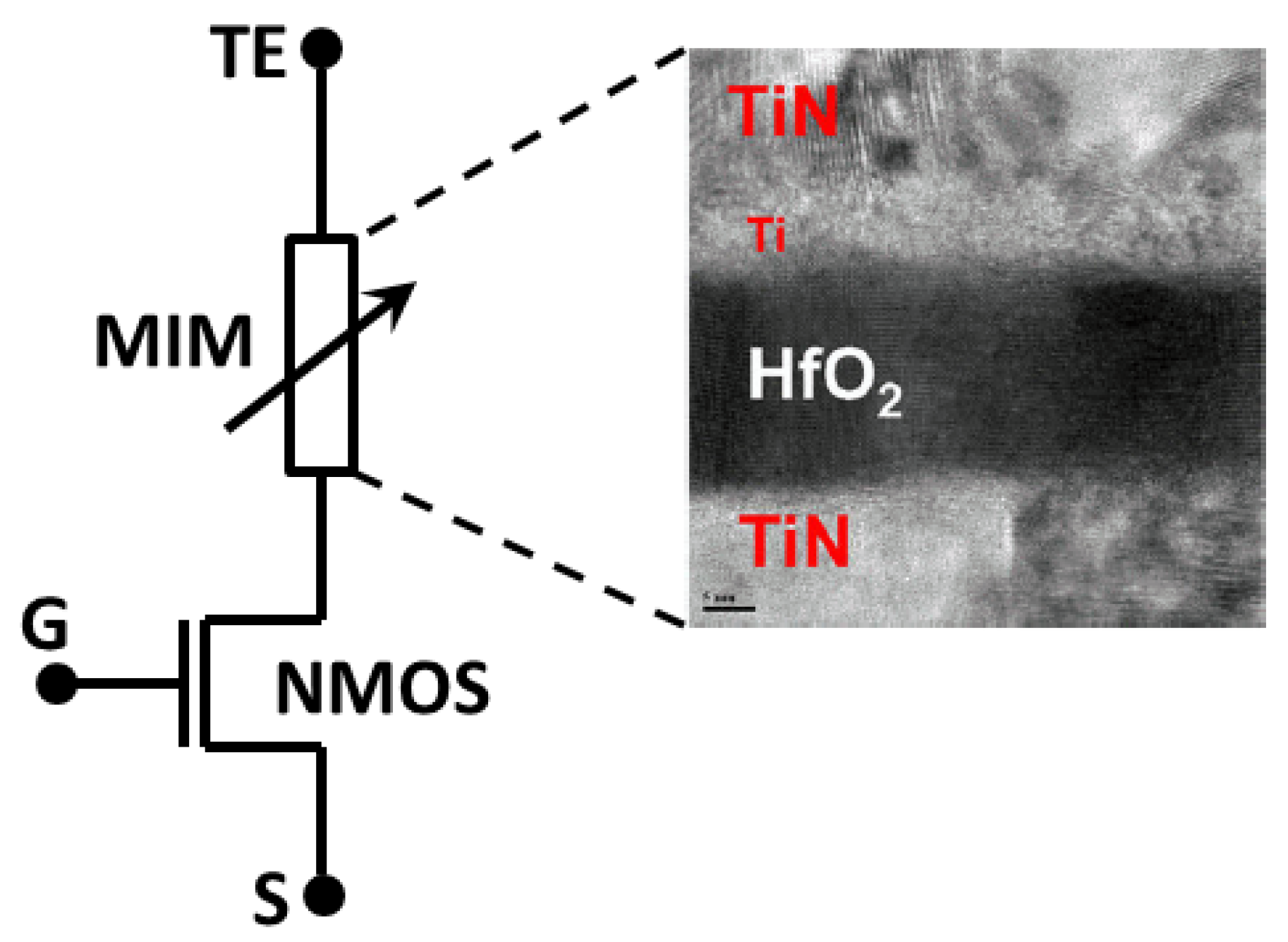
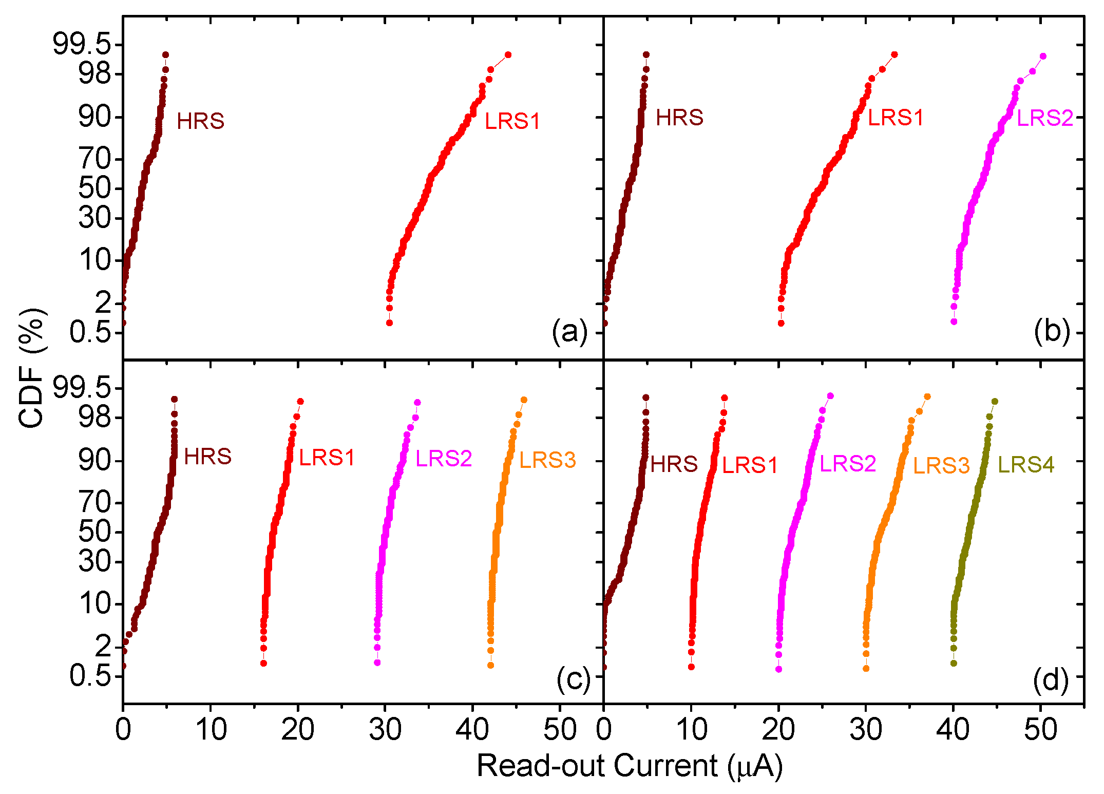
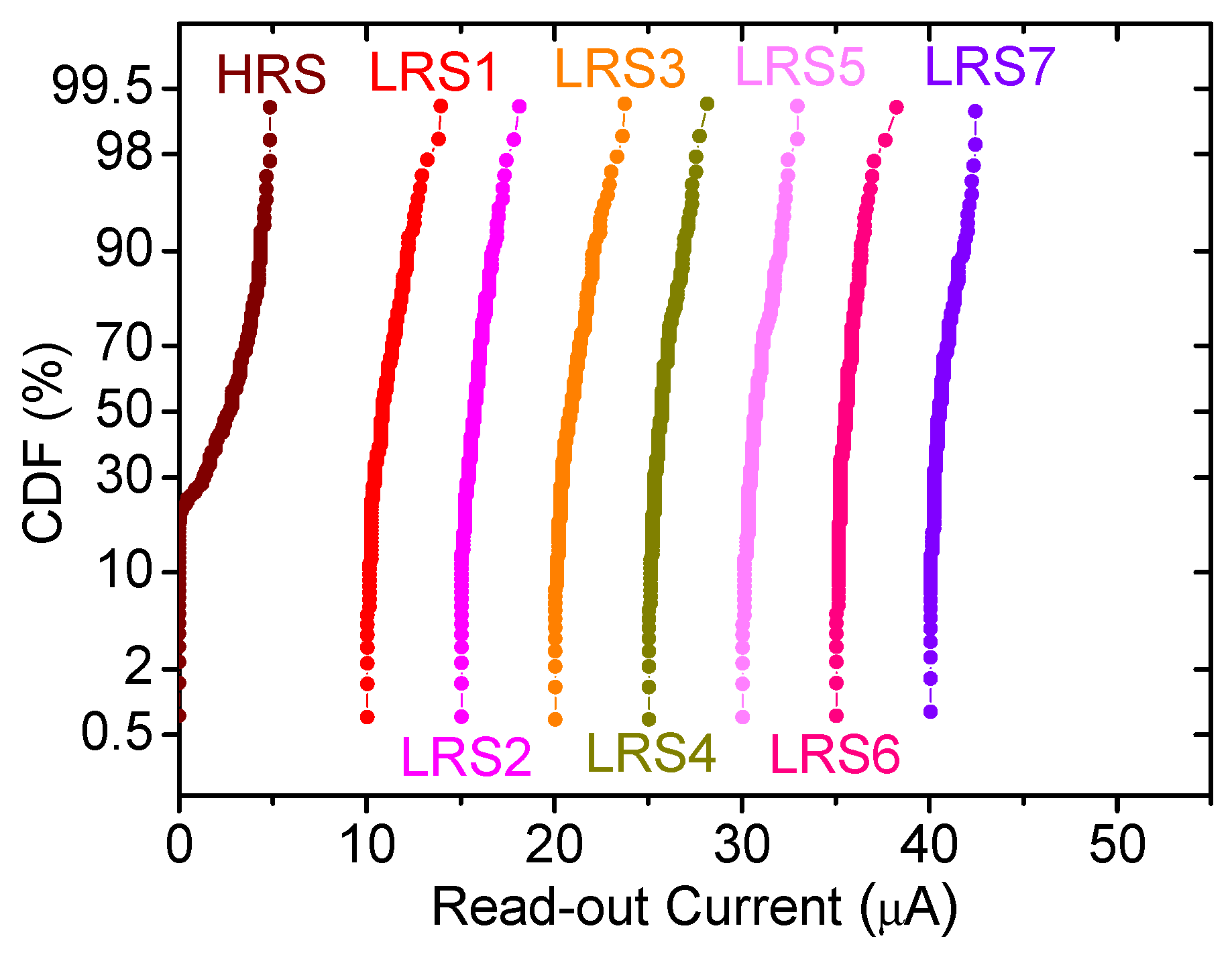
2. Device Fabrication and Measurement Set-Up, a Multilevel Approach

The devices used to define experimentally the different sets of conductance levels (2, 3, 4, 5, and 8), in order to implement the quantized weight values for the artificial synapses included in the ANN architectures considered here, are 1T1R RRAM cells integrated in 4-kbit arrays [31]. These resistive switching cells are constituted by a NMOS transistor (manufactured in 0.25 μ m CMOS technology) connected in series to a metal–insulator–metal (MIM) structure placed on the metal line 2 of the CMOS process (Figure 1). Such a MIM structure consists of a T i N / H f O 2 / T i / T i N stack with 150 nm TiN top and bottom electrode layers deposited by magnetron sputtering, a 7 nm Ti layer (under the TiN top electrode) and a 8 nm H f O 2 layer grown by atomic layer deposition (ALD) [32]. The MIM structures have an area of about 0.4 μ m 2 . The endurance and retention of these devices has been studied in order to show the viability of this technology both for memory and neuromorphic applications [11,33,34].
The algorithms employed to program the conductive levels on the devices are write-verify approaches. The cost in time of such approaches is justified due to the fact that the ANNs implemented aim to perform just the inference phase, where an accurate definition of the conductive levels is crucial. Most of the sets of conductive levels considered (in particular, 2, 3, 4, and 5) were defined by using the well-known Multilevel Incremental Step Pulse with Verify Algorithm (M-ISPVA) [35], which tunes the current target ( I t r g ) and gate voltage ( V g ) parameters during set operations to achieve each conductive level within a specific set of conductive levels. To do so, we employ different pairs of parameters that allow the control of the redox chemical reaction kinetics that lead to the device conductance variation produced by the growth and destruction of conductive filaments that bridge the electrodes through the device dielectric. During the M-ISPVA programming, a sequence of increasing voltage amplitude pulses are applied either on the terminal connected to the top electrode of the MIM structure, during set operations, or on the source terminal of the transistor, during reset operations. In contrast, placing eight conductive levels in a read-out current range of about 50 μ A requires a more advanced implementation. This algorithm, already tested in [36] and known as Incremental Gate Voltage and Verify Algorithm (IGVVA), keeps constant the pulse amplitude applied on the terminal connected to the top electrode of the MIM structure during set operations and increases step by step the V g value until I t r g is achieved. The cumulative distribution functions (CDFs) of the read-out currents measured on 128 RRAM devices for different sets of conductive levels, namely: 2, 3, 4, and 5; are shown in Figure 2. We perform the study of read-out current distributions since it directly characterizes the device conductance, which is the key magnitude to quantize in order to mimic biological synapses plasticity in neuromorphic circuits. Notice that the separation between the distributions is essential to avoid overlapping in the quantized levels. As it will be shown below, we will study the quantization in the synaptic weights of different neural networks to assess its influence on the network performance.
By tuning the M-ISPVA parameters, the definition of several non-overlapping conductive levels, up to five, can be effectively performed, see Figure 2. In addition, Figure 3 shows the current CDFs corresponding to eight conductive levels defined by using the IGVVA.
A strong reduction of the device-to-device variability allows to define extremely narrow distributions and, therefore, eight non-overlapping conductive levels in a current range of less than 50 μ A, see Figure 3. The exact determination of the device conductivity would require the detailed calculation of the current for a determined bias, this can be performed following different simulation schemes [37,38].

3. ANN Architecture Analysis, the Role of Quantization

As pointed out above, ANN have resurfaced and gained prominence due to several factors; among them, the emergence and fast development of DNNs. Because of this, the main features of DNN architectures have been characterized in-depth in the last few years [39,40,41,42]. Convolutional Neural Networks (CNN) are an alternative type of DNNs widely employed to tackle image recognition problems. Image recognition is a key activity in what we call perception; at this task, efficiency implies a fast and highly parallel data processing [43].

3.1. Convolutional Neural Networks

CNNs are based on the application of convolution functions: a mathematical operation on two functions ( f 1 and f 2 ) that produces a third function ( f 1 × f 2 ) expressing how the shape of one of them is modified by the other. It is defined as the integral of the product of the two functions after one is reversed and shifted. Then, the integral is evaluated for all the possible values of the shift producing the convolution function [44].
A CNN (Figure 4) starts with a convolutional layer which requires a minimum of three parameters: stride, kernel and filter. Stride is the number of pixels shifts over the input matrix (e.g., when the stride is 2, then, we move the filters 2 pixel at a time). The kernel is a shared small weight matrix often used for pre-processing operations such as blurring, sharpening, embossing, or edge detection. Finally, several different filters can be used, thus having a multidimensional layer. Each filter is initialized differently, and can, therefore, find better or worse image features. After a convolutional layer, a pooling layer is generally applied to reduce the size of the image combining neighboring pixels of a certain image area into a single representative value. In our case, we used the maximum value of all the considered neighboring pixels, constructing a max-pooling layer. The backpropagation algorithm used in the CNN is in charge of reducing the value of inefficient filters while promoting those that are useful for the classification task [45]. As a final step in the CNN, a MLP is attached. To do this, the pooled features of the last pooling layer are flattened. The MLP can have its own architecture with various hidden layers.

3.2. Quantization Process

ANN synaptic weights were quantized to a fixed number of levels during inference. The quantization process is based on a quantile-based discretization function. All weights belonging to the same bin will have the same value: the average for the given bin. This process is coherent with the experimental multilevel scheme we have presented for the reference technology we are considering. The quantization process is used locally in each layer, that is, for the set of weights used as input in a given layer.

4. Experiments and Results

We designed several experiments divided into two main groups: fully dense multilayer perceptron, called MLP, and convolutional neural networks, called CNN, as detailed in Section 3. The neural networks used in this manuscript were trained using the default parameter values of the keras/tensorflow implementation (see Table 1 for a summary of the parameters used) without any regulation techniques or dropout method [44]. We selected categorical accuracy as the comparison metric between approaches. This metric calculates the frequency in which the prediction matches the labeled data [46,47]. For both sets of experiments, input data (both training and test) were first binarized, being 0 those values lower than a threshold of 0.1 , and 1 otherwise.
Although the experimental multilevel approach consisted of quantization on 2, 3, 4, 5, and 8 levels, we have considered all the possibilities in the 2–8 interval at the simulation level to sweep all the possibilities and enhance our study. We have interpolated the distance between levels accounting for the data we have for the multilevel schemes experimentally fulfilled.

4.1. MLP Architecture

We studied both deep and shallow fully dense architectures. The final dense layer of all neural networks has a s o f t m a x activation layer attached, while the hidden layers have a relu activation layer after each of them. We experimented with the customization of two parameters to create different architectures: the number of hidden layers (ranging from 1 to 4) and the number of neurons per layer (ranging from 8 to 128).

4.2. CNN Architecture
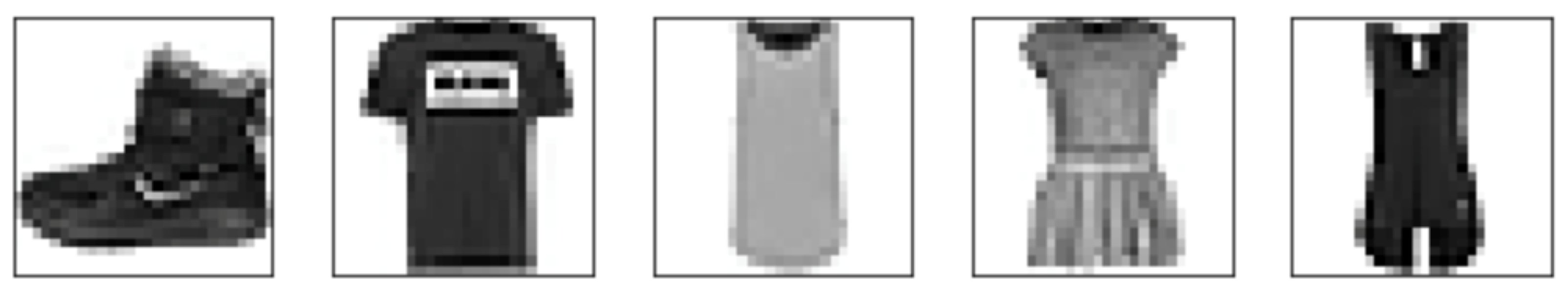
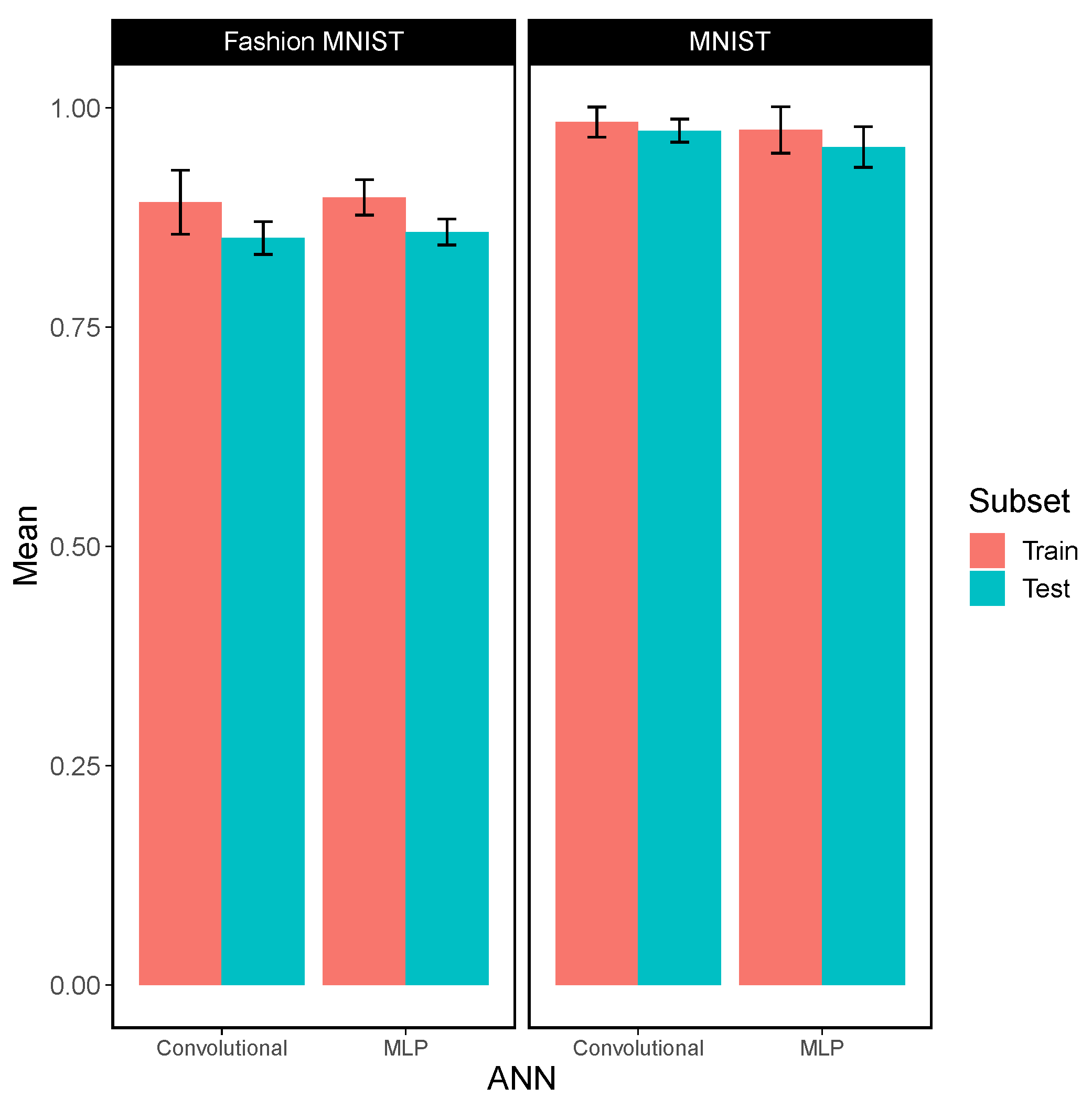
For the CNN experiments, we customized the CNN explained in Section 3.1: (1) number of convolutional layers (ranging from 1 to 3), (2) the number of filters used (ranging from 8 to 32), (3) size of the pooling matrix (ranging from 2 × 2 to 8 × 8 ), and (4) number of neurons in the hidden layer (ranging from 8 to 128). All convolutional layers are followed by an activation layer using the relu function. Only one hidden layer is explored in the MLP within the CNN since the previous layers are built to cope with the data set complexity. For all the experiments in this set we used a 3 × 3 kernel matrix. The CNN also uses a SGD optimizer with the same configuration mentioned for the MLP experiments.
The total number of synapses is, in general, higher for MLP architectures compared to CNN architectures, as seen in Figure 5. This is due to the convolutional and pooling layers incorporated in the architecture that preprocess the input data, reducing the complexity before the subsequent application of the dense layer, thus reducing the overall number of synapses.

4.3. Datasets

We used two datasets for our quantization study: MNIST [48] and Fashion MNIST [49]. The MNIST image dataset [48] is composed of 28 × 28 grayscale pixel images of 70,000 handwritten digits (labeled in the interval [0, 9]), divided into a training set (60,000 images) and a test set (10,000 images), see Figure 6.
The Fashion MNIST image dataset [49] also consists of 70,000 28 × 28 grayscale images in 10 classes (T-shirt/top, Trouser, Pullover, Dress, Coat, Sandal, Shirt, Sneaker, Bag and Ankle boot), divided into a training set (60,000 images) and a test set (10,000 images), see Figure 7. We chose to use the Fashion MNIST dataset since their authors claim that this dataset is more complex to learn than the original MNIST and better represent real-world tasks [49].
The architectures of both MNIST and Fashion MNIST networks are the same as they have the same input and output shapes.

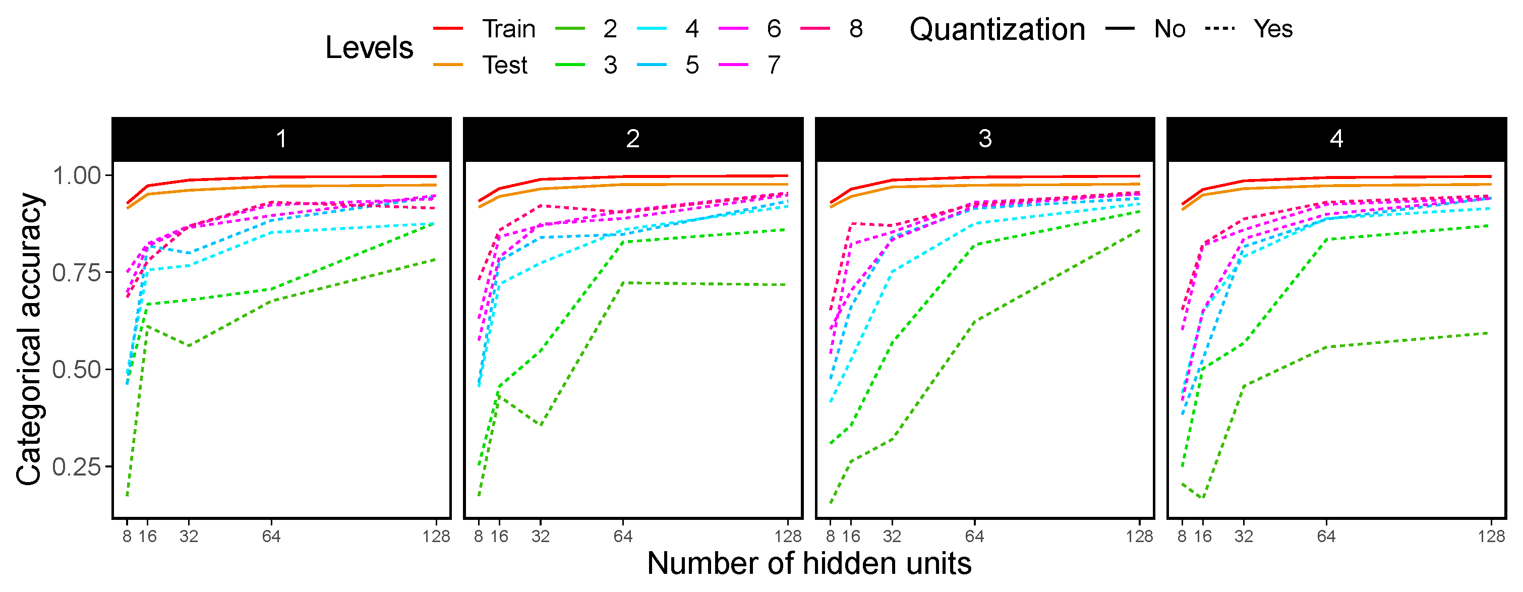
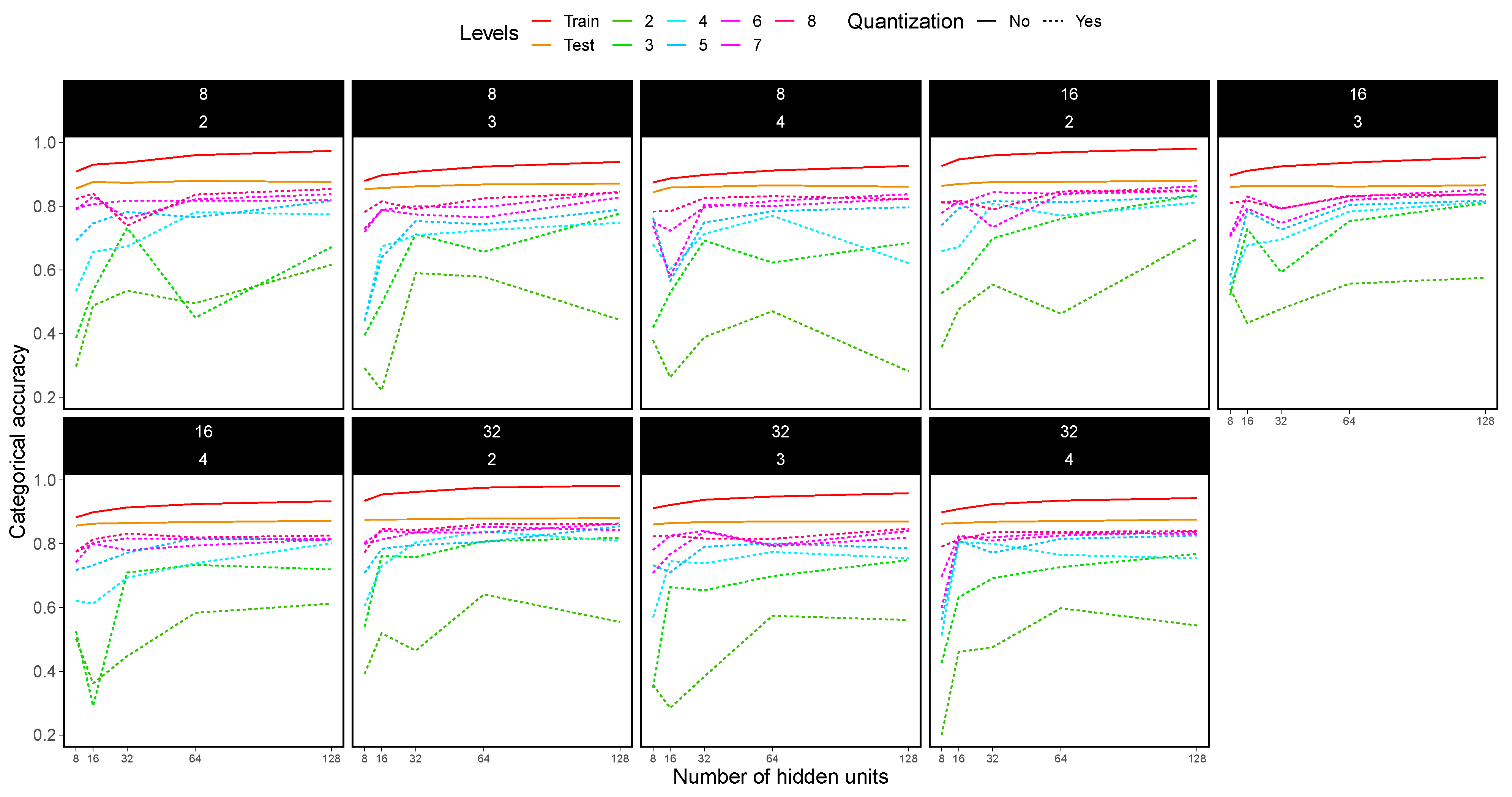
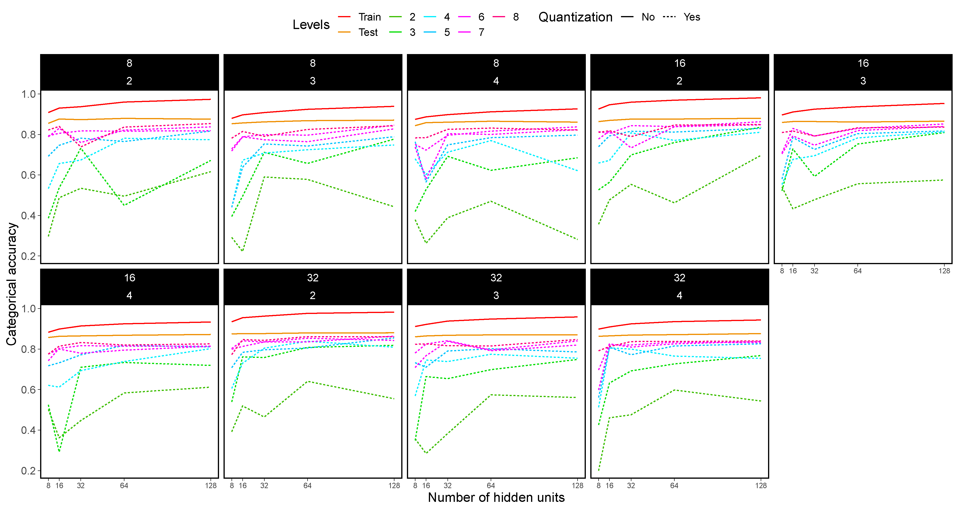
4.4. MLP Experimental Results

As introduced in Section 4.1, we experimented with different network configurations. For each configuration, we trained and tested with full floating-point precision. We also tested the neural network reducing the precision in the inference phase from 2 to 8 levels, to test its accuracy. Results are shown in Figure 8 for the MNIST dataset and in Figure 9 for the Fashion MNIST dataset.
Analyzing the experimentation results, we can infer that reducing the precision from float32 to low levels of precision (2 or 3 levels) highly impacts the overall accuracy in both datasets. When the number of quantization levels is higher (from 4 to 8 levels), the difference from the accuracy obtained using full float precision is reduced, particularly when the number of hidden units (neurons) used in each hidden layer is increased. It also seems that the minimum number of hidden units per hidden layer needs to be at least 64 in order to let a quantized MLP be comparable to the float32 precision accuracy in both training and test data.

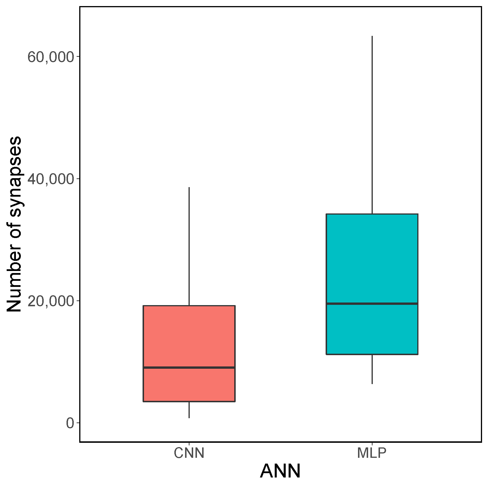
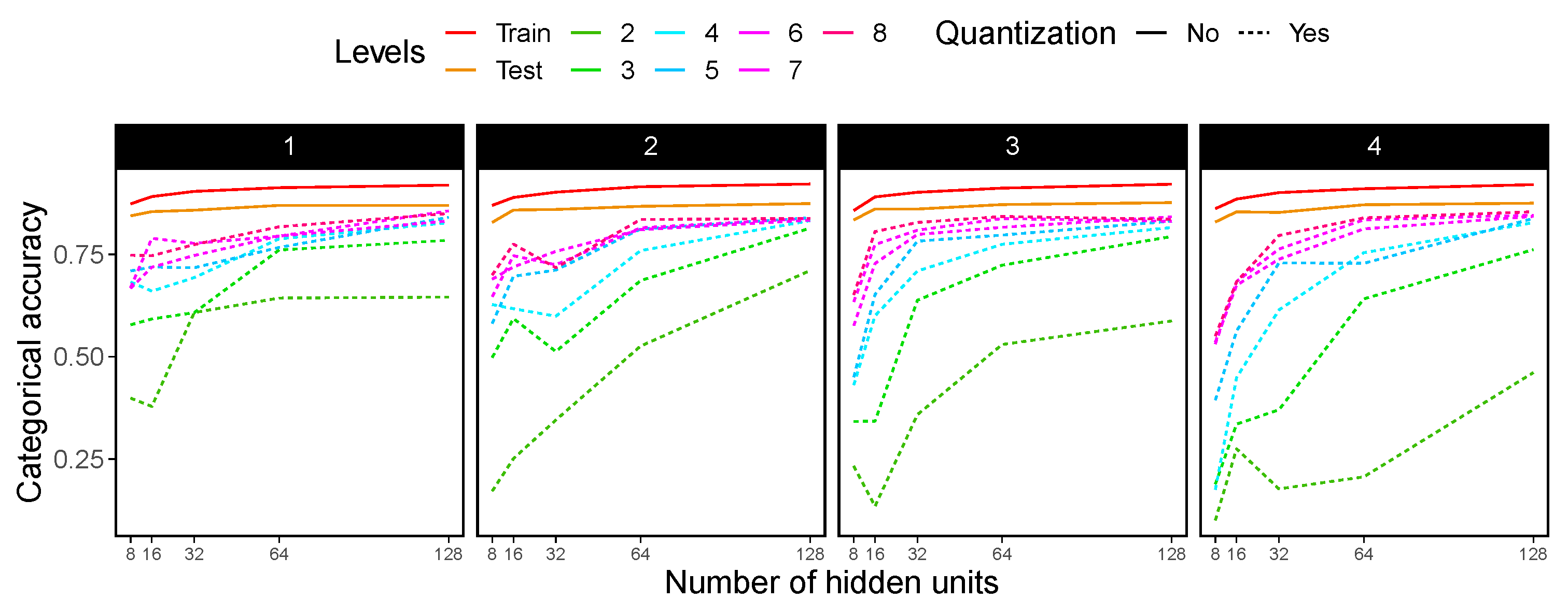
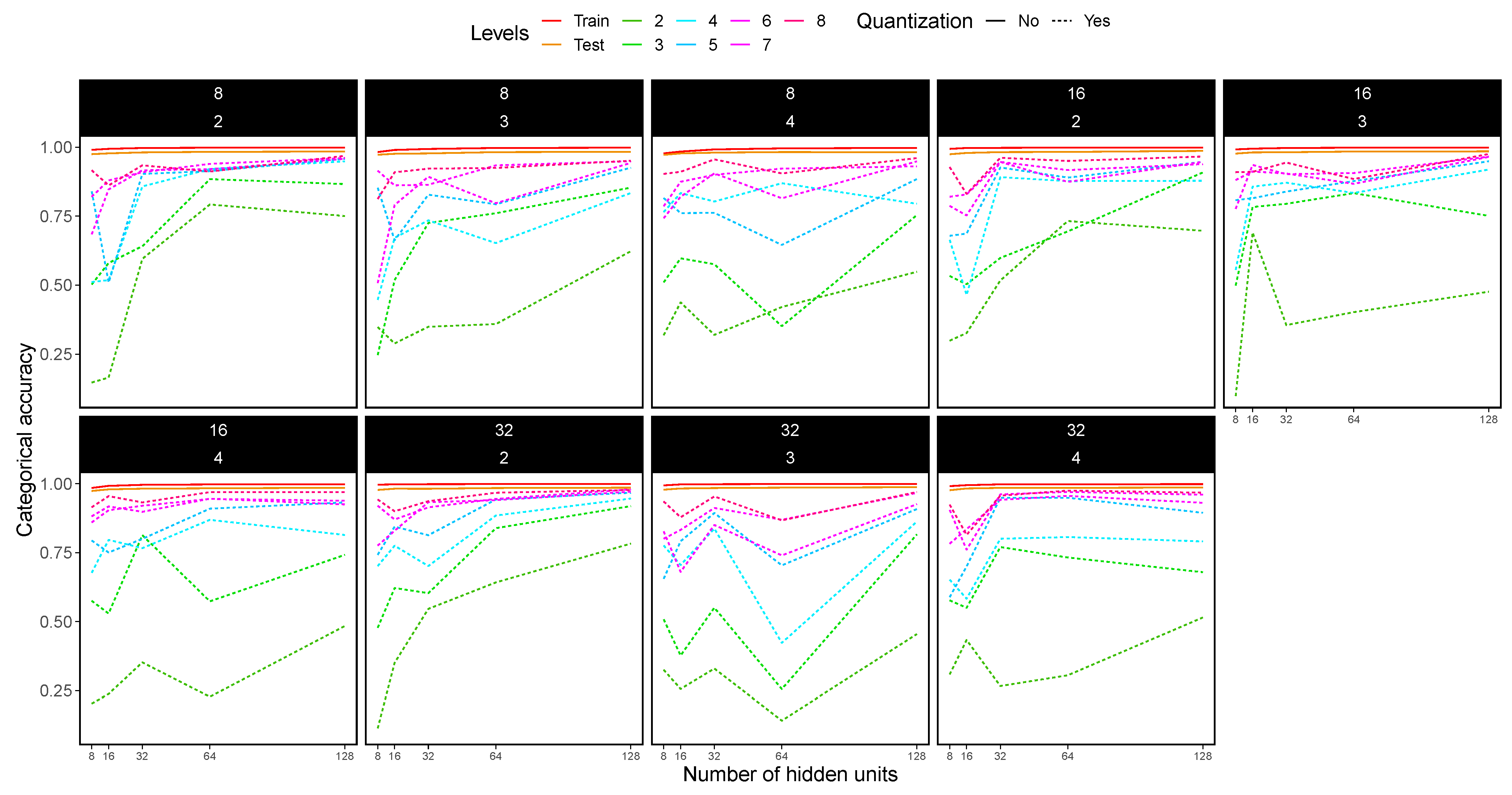
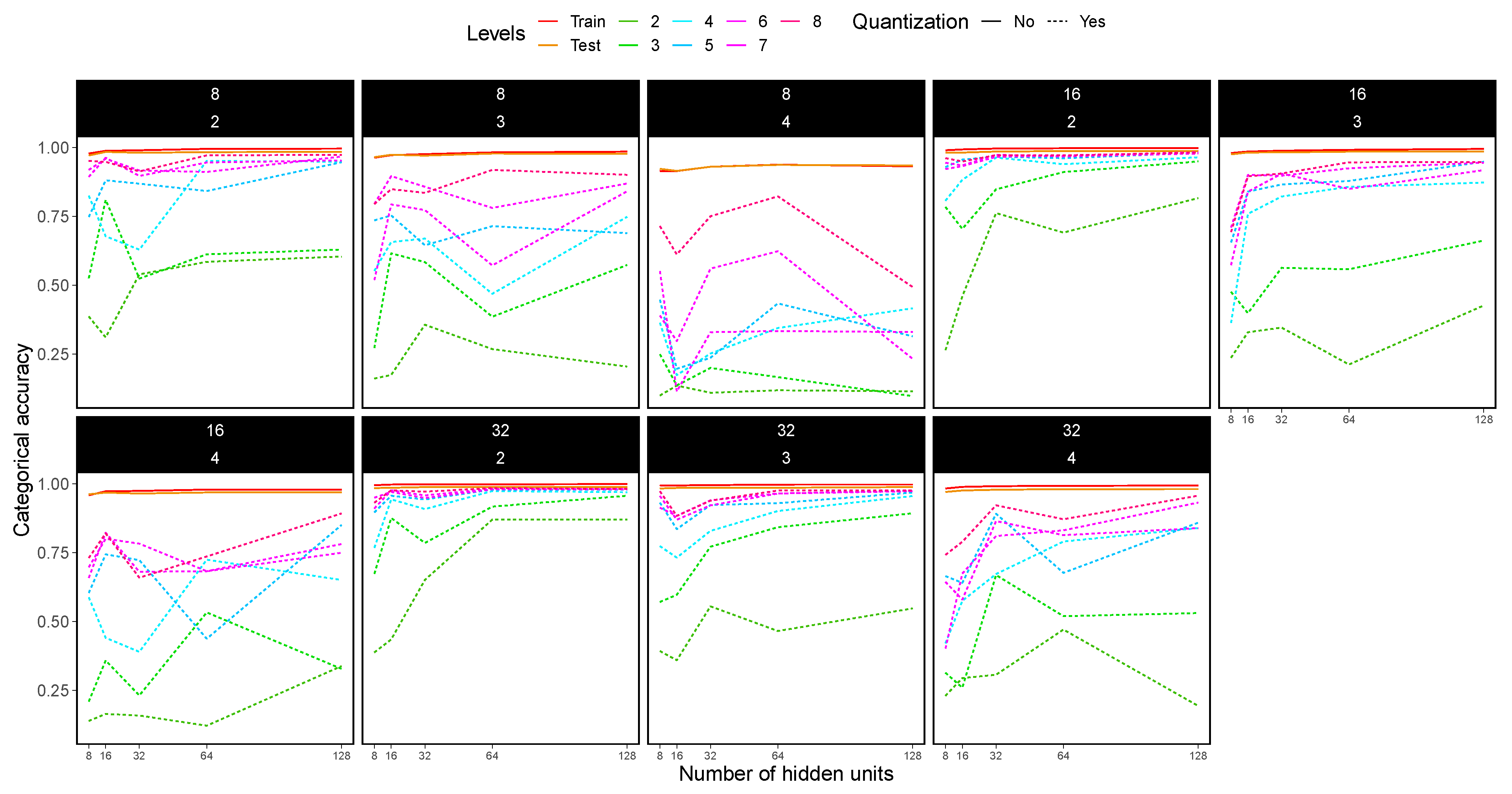
4.5. CNN Experimental Results

As introduced in Section 4.2, we also experimented using convolutional neural networks. The results show in Figure 10 the 1-CNN (one set of convolutional layer + pooling layer) using the MNIST dataset, in Figure 11 the 2-CNN is shown (two sequential sets of convolutional layers + pooling layer) using the MNIST, in Figure 12 the 1-CNN is shown again making use of the Fashion MNIST dataset and in Figure 13, the 2-CNN results are shown using the Fashion MNIST dataset.
The obtained results suggest that when the number of conductance levels used is above 5, the CNNs share a common trend with the float 32 approach, but with a slight reduction in categorical accuracy. MNIST dataset, as opposed to the Fashion MNIST dataset, is greatly affected by the CNN architecture, particularly before the flattened and fully dense layers.
The Fashion MNIST dataset is harder to predict (Figure 14) than the simpler MNIST dataset, as suggested by their authors [49]. Performing a Kruskal–Wallis rank-sum test to these data, we obtained a statistically significant difference (p-value = 1.02 × 10 5 ) between the MLP and the CNN results in the test data for MNIST, supporting the idea that CNNs perform better in image domains. The significance obtained for its counterpart in the Fashion MNIST dataset (p-value = 0.147) is low, but not low enough to be statistically significant.
It is remarkable that for both databases, and in the two types of neural networks under consideration, reasonably similar results are obtained for quantizations with 6, 7 and 8 levels. This is not a minor issue since the reduction of the number of levels allows a less complex electronic circuitry to manage memristor quantization, and also permits a greater separation of the average values in the conductance interval employed to implement the synaptic weights. This latter consideration can lead to less overlapping of the conductance levels, and therefore, to a more precise network operation. It is also important to highlight that there is a long way to go in the study and optimization of the network size, since it is clear that for a low number of neurons in the hidden layers, and for quantization strategies with very few levels, the accuracy drops off significantly. All these considerations are reflected upon the size of crossbar arrays and the consequent matrix-vector multiplication circuits needed for the hardware implementation of these neural networks. As it is usual, a trade-off has to be considered.
Overfitting is a common problem in the field of neural networks and it is spotted also in our results (Figure 14). Since our main goal is to compare the neural network behavior with different precision levels, we did not use any regulation techniques or dropout methods [44] to avoid it. However, due to the intrinsic variability of memristors linked in their stochastic operation, overfitting could be reduced significantly in comparison with software-based networks with continuous synaptic weights.
In the CNN realm, an efficient design of the convolutional layers might be the way to go to optimize the network hardware. The silicon area could be reduced if the hidden dense neural layer is optimized, due to the implications in the number of synapses that a shortening in the number of neurons can produce. In this case, even for the lower number of neurons in the hidden layer, the accuracy difference between the quantized and non-quantized cases is lower than in the other network type. Therefore, a quantized CNN approach to image recognition seems to be more appropriate (at least more flexible) from the hardware design viewpoint. Future work on this subject could be linked, among other issues, to the effects of variability on the memristive devices on the performance of the neural networks under study here.

5. Conclusions

An in-depth study of the influence of the number of conductance levels in quantized neural networks based on memristors has been performed. Different types of networks (multilayer-perceptron and convolutional) have been considered under a variety of features, such as the number of levels in the synaptic weight quantization process, the number of neurons in the hidden layers of the network topology, the image databases, the number of convolutional layers, etc. An exhaustive analysis was performed that led us to know that neural networks using a low number of synaptic weight levels require deeper and wider network architectures than those using higher precision programming algorithms. Different variables have to be taken into account in the network optimization since the number of quantized levels, the number of hidden layers and the number of neurons per hidden layers are closely related in determining the accuracy; therefore, a deep characterization is needed in each particular case prior to step in a hardware implementation process. The obtained results support the use of CNN for image domains, since convolutional layers perform a feature extraction process that reduces the complexity and the number of synaptic weights needed to achieve a neural network full potential. Thus, by reducing the number of synaptic weights needed, we can reach a comparable accuracy to their conventional multilayered-perceptron counterparts.

Author Contributions

Conceptualization, J.B.R., R.R.-Z. and C.W.; software and neural network analysis, R.R.-Z.; measurements and data analysis, E.P.; original draft preparation, review and editing, J.B.R., F.J.-M., C.W. All authors have read and agreed to the published version of the manuscript.

Funding

The authors acknowledge financial support by the German Research Foundation (DFG) in the frame of research group FOR2093, the Spanish Ministry of Science and the FEDER program through projects TEC2017-84321-C4-3-R, Consejería de Conocimiento, Investigación y Universidad, Junta de Andalucía and European Regional Development Fund (ERDF) under projects A-TIC-117-UGR18, as well as the Spanish Ministry of Science, Innovation and Universities under project RTI2018-098983-B-I00.

Data Availability Statement

The datasets generated during and/or analysed during the current study are available from the corresponding author on reasonable request.

Conflicts of Interest

The authors declare no conflict of interest.

References

  1. Krestinskaya, O.; James, A.P.; Chua, L.O. Neuromemristive Circuits for Edge Computing: A Review. IEEE Trans. Neural Netw. Learn. Syst. 2020, 31, 4–23. [Google Scholar] [CrossRef] [Green Version]
  2. Jeong, H.; Shi, L. Memristor devices for neural networks. J. Phys. Appl. Phys. 2018, 52, 023003. [Google Scholar] [CrossRef]
  3. Prezioso, M.; Merrikh-Bayat, F.; Hoskins, B.; Adam, G.; Likharev, K.; Strukov, D. Training and operation of an integrated neuromorphic network based on metal-oxide memristors. Nature 2015, 521, 7550. [Google Scholar] [CrossRef] [PubMed] [Green Version]
  4. Lanza, M.; Wong, H.S.P.; Pop, E.; Ielmini, D.; Strukov, D.; Regan, B.C.; Larcher, L.; Villena, M.A.; Yang, J.J.; Goux, L.; et al. Recommended Methods to Study Resistive Switching Devices. Adv. Electron. Mater. 2019, 5, 1800143. [Google Scholar] [CrossRef] [Green Version]
  5. Tang, J.; Yuan, F.; Shen, X.; Wang, Z.; Rao, M.; He, Y.; Sun, Y.; Li, X.; Zhang, W.; Li, Y.; et al. Bridging Biological and Artificial Neural Networks with Emerging Neuromorphic Devices: Fundamentals, Progress, and Challenges. Adv. Mater. 2019, 31, 1902761. [Google Scholar] [CrossRef] [PubMed]
  6. Xia, Q.; Berggren, K.K.; Likharev, K.; Strukov, D.B.; Jiang, H.; Mikolajick, T.; Querlioz, D.; Salinga, M.; Erickson, J.; Pi, S.; et al. Roadmap on emerging hardware and technology for machine learning. Nanotechnology 2020, 32, 012002. [Google Scholar]
  7. Yan, B.; Li, B.; Qiao, X.; Xue, C.X.; Chang, M.F.; Chen, Y.; Li, H.H. Resistive Memory-Based In-Memory Computing: From Device and Large-Scale Integration System Perspectives. Adv. Intell. Syst. 2019, 1, 1900068. [Google Scholar] [CrossRef] [Green Version]
  8. Manukian, H.; Traversa, F.L.; Ventra, M.D. Accelerating Deep Learning with Memcomputing. Neural Netw. 2019, 110, 1–7. [Google Scholar] [CrossRef] [PubMed] [Green Version]
  9. Carbajal, J.P.; Dambre, J.; Hermans, M.; Schrauwen, B. Memristor Models for Machine Learning. Neural Comput. 2015, 27, 725–747. [Google Scholar] [CrossRef]
  10. Caravelli, F.; Carbajal, J. Memristors for the Curious Outsiders. Technologies 2018, 6, 118. [Google Scholar] [CrossRef] [Green Version]
  11. Aldana, S.; Pérez, E.; Jiménez-Molinos, F.; Wenger, C.; Roldán, J.B. Kinetic Monte Carlo analysis of data retention in Al:HfO2-based resistive random access memories. Semicond. Sci. Technol. 2020, 35, 115012. [Google Scholar] [CrossRef]
  12. Villena, M.; Roldan, J.; Jimenez-Molinos, F.; Miranda, E.; Suñé, J.; Lanza, M. SIM2RRAM: A physical model for RRAM devices simulation. J. Comput. Electron. 2017, 16, 1095–1120. [Google Scholar] [CrossRef]
  13. Pérez, E.; Maldonado, D.; Acal, C.; Ruiz-Castro, J.; Alonso, F.; Aguilera, A.; Jiménez-Molinos, F.; Wenger, C.; Roldán, J. Analysis of the statistics of device-to-device and cycle-to-cycle variability in TiN/Ti/Al:HfO2/TiN RRAMs. Microelectron. Eng. 2019, 214, 104–109. [Google Scholar] [CrossRef]
  14. Roldán, J.B.; Alonso, F.J.; Aguilera, A.M.; Maldonado, D.; Lanza, M. Time series statistical analysis: A powerful tool to evaluate the variability of resistive switching memories. J. Appl. Phys. 2019, 125, 174504. [Google Scholar] [CrossRef]
  15. Acal, C.; Ruiz-Castro, J.; Aguilera, A.; Jiménez-Molinos, F.; Roldán, J. Phase-type distributions for studying variability in resistive memories. J. Comput. Appl. Math. 2019, 345, 23–32. [Google Scholar] [CrossRef]
  16. Zheng, N.; Mazumder, P. Learning in Energy-Efficient Neuromorphic Computing: Algorithm and Architecture Co-Design; Wiley: Hoboken, NJ, USA, 2019. [Google Scholar]
  17. Chen, J.; Wu, H.; Gao, B.; Tang, J.; Hu, X.S.; Qian, H. A Parallel Multibit Programing Scheme With High Precision for RRAM-Based Neuromorphic Systems. IEEE Trans. Electron Devices 2020, 67, 2213–2217. [Google Scholar] [CrossRef]
  18. Wenger, C.; Zahari, F.; Mahadevaiah, M.K.; Pérez, E.; Beckers, I.; Kohlstedt, H.; Ziegler, M. Inherent Stochastic Learning in CMOS-Integrated HfO2 Arrays for Neuromorphic Computing. IEEE Electron Device Lett. 2019, 40, 639–642. [Google Scholar] [CrossRef]
  19. Woo, J.; Moon, K.; Song, J.; Kwak, M.; Park, J.; Hwang, H. Optimized Programming Scheme Enabling Linear Potentiation in Filamentary HfO2 RRAM Synapse for Neuromorphic Systems. IEEE Trans. Electron Devices 2016, 63, 5064–5067. [Google Scholar] [CrossRef]
  20. Sun, S.; Wu, H.; Xiang, L. City-Wide Traffic Flow Forecasting Using a Deep Convolutional Neural Network. Sensors 2020, 20, 421. [Google Scholar] [CrossRef] [Green Version]
  21. Geng, Z.; Wang, Y. Automated design of a convolutional neural network with multi-scale filters for cost-efficient seismic data classification. Nat. Commun. 2020, 11, 3311. [Google Scholar] [CrossRef] [PubMed]
  22. Bhattacharya, S.; Somayaji, S.R.K.; Gadekallu, T.R.; Alazab, M.; Maddikunta, P.K.R. A review on deep learning for future smart cities. Internet Technol. Lett. 2020, e187. [Google Scholar] [CrossRef]
  23. Kattenborn, T.; Eichel, J.; Fassnacht, F.E. Convolutional Neural Networks enable efficient, accurate and fine-grained segmentation of plant species and communities from high-resolution UAV imagery. Sci. Rep. 2019, 9, 17656. [Google Scholar] [CrossRef] [PubMed]
  24. Webb, S. Deep learning for biology. Nature 2018, 554, 555–557. [Google Scholar] [CrossRef] [Green Version]
  25. Tang, B.; Pan, Z.; Yin, K.; Khateeb, A. Recent Advances of Deep Learning in Bioinformatics and Computational Biology. Front. Genet. 2019, 10, 214. [Google Scholar] [CrossRef] [Green Version]
  26. Wu, S.; Zhao, W.; Ghazi, K.; Ji, S. Convolutional neural network for efficient estimation of regional brain strains. Sci. Rep. 2019, 9, 17326. [Google Scholar] [CrossRef] [Green Version]
  27. Esteva, A.; Robicquet, A.; Ramsundar, B.; Kuleshov, V.; DePristo, M.; Chou, K.; Cui, C.; Corrado, G.; Thrun, S.; Dean, J. A guide to deep learning in healthcare. Nat. Med. 2019, 25, 24–29. [Google Scholar] [CrossRef]
  28. Piccialli, F.; Somma, V.D.; Giampaolo, F.; Cuomo, S.; Fortino, G. A survey on deep learning in medicine: Why, how and when? Inf. Fusion 2021, 66, 111–137. [Google Scholar] [CrossRef]
  29. Zhang, Y.; Cui, M.; Shen, L.; Zeng, Z. Memristive Quantized Neural Networks: A Novel Approach to Accelerate Deep Learning On-Chip. IEEE Trans. Cybern. 2019, 1–13. [Google Scholar] [CrossRef] [PubMed]
  30. Hu, X.; Duan, S.; Chen, G.; Chen, L. Modeling affections with memristor-based associative memory neural networks. Neurocomputing 2017, 223, 129–137. [Google Scholar] [CrossRef]
  31. Zambelli, C.; Grossi, A.; Olivo, P.; Walczyk, D.; Bertaud, T.; Tillack, B.; Schroeder, T.; Stikanov, V.; Walczyk, C. Statistical analysis of resistive switching characteristics in ReRAM test arrays. In Proceedings of the 2014 International Conference on Microelectronic Test Structures (ICMTS), Udine, Italy, 24–27 March 2014; pp. 27–31. [Google Scholar] [CrossRef]
  32. Grossi, A.; Perez, E.; Zambelli, C.E.A. Impact of the precursor chemistry and process conditions on the cell-to-cell variability in 1T-1R based HfO2 RRAM devices. Sci. Rep. 2018, 8, 11160. [Google Scholar] [CrossRef] [PubMed] [Green Version]
  33. Milo, V.; Zambelli, C.; Olivo, P.; Pérez, E.; Mahadevaiah, M.K.; Ossorio, O.G.; Wenger, C.; Ielmini, D. Multilevel HfO2-based RRAM devices for low-power neuromorphic networks. APL Mater. 2019, 7, 081120. [Google Scholar] [CrossRef] [Green Version]
  34. Pérez, E.; Ossorio, O.G.; Dueñas, S.; Castán, H.; García, H.; Wenger, C. Programming Pulse Width Assessment for Reliable and Low-Energy Endurance Performance in Al: HfO2-Based RRAM Arrays. Electronics 2020, 9, 864. [Google Scholar] [CrossRef]
  35. Pérez, E.; Zambelli, C.; Mahadevaiah, M.K.; Olivo, P.; Wenger, C. Toward Reliable Multi-Level Operation in RRAM Arrays: Improving Post-Algorithm Stability and Assessing Endurance/Data Retention. IEEE J. Electron Devices Soc. 2019, 7, 740–747. [Google Scholar] [CrossRef]
  36. Milo, V.; Anzalone, F.; Zambelli, C.; Pérez, E.; Mahadevaiah, M.; Ossorio, O.; Olivo, P.; Wenger, C.; Ielmini, D. Optimized programming algorithms for multilevel RRAM in hardware neural networks. In Proceedings of the 2021 IEEE International Reliability Physics Symposium (IRPS), Monterey, CA, USA, 21–25 March 2021. [Google Scholar]
  37. González-Cordero, G.; Jiménez-Molinos, F.; Roldán, J.B.; González, M.B.; Campabadal, F. In-depth study of the physics behind resistive switching in TiN/Ti/HfO2/W structures. J. Vac. Sci. Technol. B 2017, 35, 01A110. [Google Scholar] [CrossRef]
  38. Aldana, S.; García-Fernández, P.; Romero-Zaliz, R.; González, M.B.; Jiménez-Molinos, F.; Gómez-Campos, F.; Campabadal, F.; Roldán, J.B. Resistive switching in HfO2 based valence change memories, a comprehensive 3D kinetic Monte Carlo approach. J. Phys. Appl. Phys. 2020, 53, 225106. [Google Scholar] [CrossRef]
  39. Bashar, A. Survey on Evolving Deep Learning Neural Network Architectures. J. Artif. Intell. Capsul. Netw. 2019, 1, 73–82. [Google Scholar] [CrossRef]
  40. Nassif, A.B.; Shahin, I.; Attili, I.; Azzeh, M.; Shaalan, K. Speech recognition using deep neural networks: A systematic review. IEEE Access 2019, 7, 19143–19165. [Google Scholar] [CrossRef]
  41. Dhillon, A.; Verma, G.K. Convolutional neural network: A review of models, methodologies and applications to object detection. Prog. Artif. Intell. 2020, 9, 85–112. [Google Scholar] [CrossRef]
  42. Zou, L.; Yu, S.; Meng, T.; Zhang, Z.; Liang, X.; Xie, Y. A technical review of convolutional neural network-based mammographic breast cancer diagnosis. Comput. Math. Methods Med. 2019, 2019. [Google Scholar] [CrossRef] [Green Version]
  43. Liu, C.; Chen, H.; Wang, S.; Liu, Q.; Jiang, Y.G.; Zhang, D.W.; Liu, M.; Zhou, P. Two-dimensional materials for next-generation computing technologies. Nat. Nanotechnol. 2020, 15, 545. [Google Scholar] [CrossRef] [PubMed]
  44. Aggarwal, C.C. Neural Networks and Deep Learning: A Textbook; Springer: Berlin/Heidelberg, Germany, 2018. [Google Scholar]
  45. Astudillo, N.M.; Bolman, R.; Sirakov, N.M. Classification with Stochastic Learning Methods and Convolutional Neural Networks. SN Comput. Sci. 2020, 1, 1–9. [Google Scholar] [CrossRef] [Green Version]
  46. Abadi, M.; Agarwal, A.; Barham, P.; Brevdo, E.; Chen, Z.; Citro, C.; Corrado, G.S.; Davis, A.; Dean, J.; Devin, M.; et al. TensorFlow: Large-Scale Machine Learning on Heterogeneous Systems. arXiv 2016, arXiv:1603.04467. [Google Scholar]
  47. Chollet, F. Keras. 2015. Available online: https://keras.io (accessed on 7 January 2021).
  48. LeCun, Y.; Cortes, C.; Burges, C. MNIST handwritten Digit Database. ATT Labs [Online]. 2010. Available online: http://yann.lecun.com/exdb/mnist (accessed on 7 January 2021).
  49. Xiao, H.; Rasul, K.; Vollgraf, R. Fashion-MNIST: A Novel Image Dataset for Benchmarking Machine Learning Algorithms. arXiv 2017, arXiv:1708.07747. [Google Scholar]
Figure 1. Circuit schematic of the 1T1R cells (G: gate terminal; S: source terminal; and TE: top electrode terminal) and cross-sectional TEM image of the metal–insulator–metal (MIM) stack.
Electronics 10 00346 g001
Figure 2. Cumulative distribution functions (CDFs) of the read-out currents measured for each set of conductive levels, namely, 2 levels (a), 3 levels (b), 4 levels (c), and 5 levels (d). The conductance levels were obtained by means of the Multilevel Incremental Step Pulse with Verify Algorithm (M-ISPVA) algorithm [35]. LRS stands for low resistance state, this means that the memristors have a low internal resistance value, and HRS stands for high resistance state. These current levels, and therefore, the device conductance, are obtained by means of different sets of algorithm parameters. In this respect, the corresponding neural network weight quantization strategies can be linked to the algorithms chosen to electrically operate the devices.
Electronics 10 00346 g002
Figure 3. CDFs of the read-out currents measured for eight levels. The conductance levels were obtained by means of the Incremental Gate Voltage and Verify Algorithm (IGVVA) algorithm [36]. LRS stands for low resistance state, this means that the memristors has a low internal resistance value, and HRS stands for high resistance state.
Electronics 10 00346 g003
Figure 4. CNN architecture. The input data are introduced into a convolutional layer (accounting for different convolutional filters to generate feature maps, that accentuate the unique features of the original image) followed by a pooling layer (that reduces the size of the image combining neighboring pixels of a certain image area into a single representative value). Multiple sets of convolutional + pooling layers can be applied as pre-processing. Finally, all outputs of the last pooling layer are flattened (from a matrix to an array) and used as inputs of a MLP.
Electronics 10 00346 g004
Figure 5. Distribution of total number of synapses for each type of artificial neural network (ANN). The boxplots show a rectangle where its bottom line corresponds to the 25th percentile (or first quartile), the top line to the 75th percentile (or third quartile) and the middle line to 50th percentile or median (the middle value). The vertical line below the box extends until the 0th percentile (the lowest data point excluding outliers), while the vertical line above the box extends until 100th percentile (the largest data point excluding outliers). In this figure, outliers were removed for visualization enhancement.
Electronics 10 00346 g005
Figure 6. Four examples the 28 × 28 pixel images of the MNIST dataset, labelled as “4”, “1”, “9” and “2” from left to right.
Electronics 10 00346 g006
Figure 7. Five examples the 28 × 28 grayscale pixel images of the Fashion MNIST dataset, labelled as “Ankle boot”, “T-shirt/top”, “T-shirt/top”, “Dress” and “Dress” from left to right.
Electronics 10 00346 g007
Figure 8. Categorical accuracy for the MNIST dataset. Experiments using 1 to 4 hidden layers, shown in each of the boxes, were used. For each hidden layer, hidden units ranging from 8 to 128 were tested (x axis). Each dashed line in the plots shows the accuracy for different quantization levels, while solid lines indicate no quantization.
Electronics 10 00346 g008
Figure 9. Categorical accuracy for the Fashion MNIST dataset. Experiments using 1 to 4 hidden layers, shown in each of the boxes, were used. For each hidden layer, hidden units ranging from 8 to 128 were tested (x axis). Each dashed line in the plots shows the accuracy for different quantization levels, while solid lines indicate no quantization.
Electronics 10 00346 g009
Figure 10. Categorical accuracy for the MNIST dataset using 1-CNN (i.e., one convolutional layer + one pooling layer). Only one hidden layer was used, with hidden units ranging from 8 to 128 (x axis). Each dashed line in the plots shows the accuracy for different quantization levels, while solid lines indicate no quantization. Each box in the figure shows a particular experiment: convolutional layer with 8, 16 and 32 filters (top number of the box) and pooling with 2 × 2 , 3 × 3 and 4 × 4 matrices (bottom number of the box).
Electronics 10 00346 g010
Figure 11. Categorical accuracy for the MNIST dataset using 2-CNN (i.e., one convolutional layer, one intermediate pooling layer, another convolutional layer and a final pooling layer). Only one hidden layer was used, with hidden units ranging from 8 to 128 (x axis). Each dashed line in the plots shows the accuracy for different quantization levels, while solid lines indicate no quantization. Each box in the figure shows a particular experiment: convolutional layer with 8, 16 and 32 filters (the top number of the box) and pooling with 2 × 2 , 3 × 3 and 4 × 4 matrices (the bottom number of the box).
Electronics 10 00346 g011
Figure 12. Categorical accuracy for the Fashion MNIST dataset using 1-CNN (i.e., one convolutional layer + one pooling layer). Only one hidden layer was used, with hidden units ranging from 8 to 128 (x axis). Each dashed line in the plots shows the accuracy for different quantization levels, while solid lines indicate no quantization. Each box in the figure shows a particular experiment: convolutional layer with 8, 16 and 32 filters (top number of the box) and pooling with 2 × 2 , 3 × 3 and 4 × 4 matrices (bottom number of the box).
Electronics 10 00346 g012
Figure 13. Categorical accuracy for the Fashion MNIST dataset using 2-CNN (i.e., one convolutional layer, one intermediate pooling layer, another convolutional layer and a final pooling layer). Only one hidden layer was used, with hidden units ranging from 8 to 128 (x axis). Each dashed line in the plots shows the accuracy for different quantization levels, while solid lines indicate no quantization. Each box in the figure shows a particular experiment: convolutional layer with 8, 16 and 32 filters (the top number of the box) and pooling with 2 × 2 , 3 × 3 and 4 × 4 matrices (the bottom number of the box).
Electronics 10 00346 g013
Figure 14. Mean categorical accuracy for MNIST and Fashion MNIST datasets using MLP and CNN, including error bars using one standard deviation.
Electronics 10 00346 g014
Table 1. Parameters used in the experiments.
Parameter NameValue
OptimizerStochastic Gradient Descent (SGD)
Learning rate0.1
Momentum0.9
Number of epochs30
Batch Size32
Validation set10%
Publisher’s Note: MDPI stays neutral with regard to jurisdictional claims in published maps and institutional affiliations.

