
Toward Autonomous UAV Localization via Aerial Image Registration
by
 , ,
, ,
Xuezhi Wang
1,* ,
,
Allison Kealy
1,
Wenchao Li
1,
Beth Jelfs
2,
Christopher Gilliam
2,
Samantha Le May
1 and
Bill Moran
3 
1
School of Science, RMIT University, Melbourne, VIC 3000, Australia
2
School of Engineering, RMIT University, Melbourne, VIC 3000, Australia
3
Department of Electrical and Electronic Engineering, University of Melbourne, Melbourne, VIC 3010, Australia
*
Author to whom correspondence should be addressed.
Electronics 2021, 10(4), 435; https://doi.org/10.3390/electronics10040435
Submission received: 22 December 2020
/
Revised: 27 January 2021
/
Accepted: 4 February 2021
/
Published: 10 February 2021
(This article belongs to the Special Issue Autonomous Navigation Systems for Unmanned Aerial Vehicles)
Abstract
:Absolute localization of a flying UAV on its own in a global-navigation-satellite-system (GNSS)-denied environment is always a challenge. In this paper, we present a landmark-based approach where a UAV is automatically locked into the landmark scene shown in a georeferenced image via a feedback control loop, which is driven by the output of an aerial image registration. To pursue a real-time application, we design and implement a speeded-up-robust-features (SURF)-based image registration algorithm that focuses efficiency and robustness under a 2D geometric transformation. A linear UAV controller with signals of four degrees of freedom is derived from the estimated transformation matrix. The approach is validated in a virtual simulation environment, with experimental results demonstrating the effectiveness and robustness of the proposed UAV self-localization system.
1. Introduction
Pure inertial navigation systems develop errors that increase with time. For long duration flights, position update from external sources (e.g., global navigation satellite system (GNSS) aiding, star tracker celestial localization systems, aerial video tracking of landmarks) is necessary to bound the inertial errors [1].
Navigation of an unmanned aerial vehicle (UAV) using georeferencing methods other than GNSS is rather challenging [2]. Available techniques include simultaneous localization and mapping (SLAM) and video odometry [3,4,5], also known as video tracking [6,7]. These techniques extract the vehicle’s relative location from the geometric scene, sometimes fusing this with the outputs of other coherent sensors onboard (e.g., data from a lidar or ultrawideband device) to build a live map incrementally via Bayesian filtering [8]. However, external reference is required if navigation is based on a global coordinate system. The idea behind this work is to implement an online image processing system that can automatically provide UAV steering controls driving the UAV into a scene of known location by comparing onboard aerial video frames with a georeferenced image. A georeferenced image may be acquired, for example, from an aerial landmark image or from Google Maps, which are prerecorded with help from external reference sources. In the literature, navigation methods of this type are referred to as vision-based navigation [9,10], indirect georeferencing [10,11], or landmark georeferencing [4,12]. Such methods aim to find ground georeference points using onboard aerial image processing and, therefore, enable the position of a vehicle on a global map to be determined in a GNSS-denied environment.
One of the key challenges of building a landmark-based UAV self-localization system is the requirement of an efficient image registration algorithm. Apart from the robustness and accuracy for affine transformations, the algorithm should be operationally autonomous with great computational efficiency, both of which are crucial properties for applications involving real-time processing. In the proposed system, handling a complex warped scene is considered less important, with the priority being that the registration algorithm must be efficient and automated to satisfy the need for real-time control and signal processing.
While area-based image registration techniques are generally more accurate and robust, their computational complexities are also higher than those of feature-point-based image registration techniques [13]. Some computationally efficient algorithms such as the enhanced correlation coefficient (ECC) maximization algorithm [14] and discrete-Fourier-transformation-based subpixel image registration [15] are also available in the literature. A more recent work by [16] describes an elastic registration method for dealing with images of different modalities and nonuniform illumination. These approaches have manifested some advanced features, such as invariant to photometric distortions in contrast and brightness that coped with a nonlinear function of parameters. Nevertheless, their overall accuracy and efficiency are highly dependent on the application and the robustness over mapping conditions is fragile compared with feature-point-based approaches in our experimental test. For feature-point-based algorithms, although the scale-invariant feature transform (SIFT) algorithm [17] may be a good candidate for this work, we found that the algorithm efficiency needed to be improved; for example, the rotational invariancy was not always reliable. The speeded up robust features (SURF) algorithm proposed in [18] has greatly rectified these problems and its efficiency is remarkable.
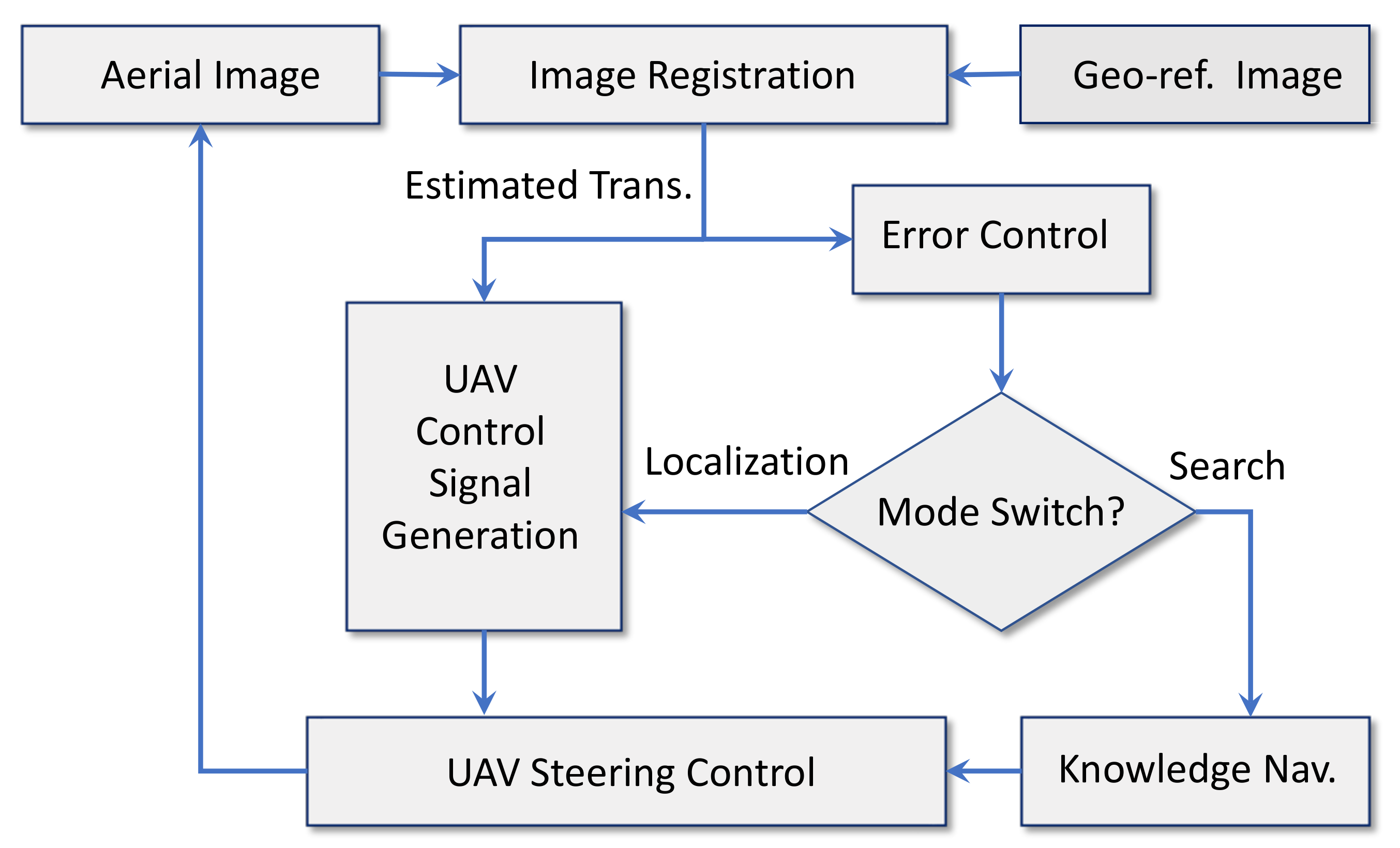
In this paper, we propose a UAV self-localization system that acquires position information by an image-registration-driven control process that recursively steers the UAV to align with the scene of a georeferenced image. As illustrated in Figure 1, at a sampling interval, an aerial image is taken by the aerial view camera onboard the UAV and is compared with a georeferenced image for similarity by an online image registration algorithm. When a common scene between the two images is found via online image registration, we estimate the associated transformation matrix. The latter contains information on how this UAV should be steered such that the dissimilarity between the image pair is minimized. The UAV control signal generator interprets the estimated transformation matrix into a series of UAV steering controls, which, in turn, drive the UAV toward the scene of the georeferenced image. The process can be seen as a first order feedback control and will be terminated if a desired registration quality is stabilized. The UAV of the proposed system has two flying modes. While in “search mode”, the UAV is navigated by an onboard inertial navigation system (INS). Once a common scene is detected, the system releases the UAV steering control to the UAV control signal generator and enters into the “locked-up self-localization mode”.
In a more generic scenario, the proposed UAV self-localization system may work on a set of georeferenced images taken on a predefined flight path and use the localization outcomes to recalibrate the onboard inertial navigation system. It is in favor of those applications where the georeferenced images contain many distinguishable features, such as the 3D localization/tracking inside a complex building, or in a low-altitude urban environment in the absence of GNSS.
In the proposed system development, we have three major contributions. First, an autonomous fast speeded-up-robust-features (SURF)-based image registration algorithm for the underlying application is designed. Second, UAV controls for the localization process are derived from the estimated transformation matrix under linear mapping. Third, we implement a virtual aerial camera and build a near-online testing platform using Google 3D Maps that enables a Monte-Carlo-based simulation to examine the performance of the proposed UAV self-localization system in terms of effectiveness, robustness, and localization accuracy. The proposed method differs from existing vision-based approaches, as it finds both the vehicle position and attitudes using the entire scene of a georeferenced image.
Following the introduction section, the automated SURF-based image registration algorithm design is described in Section 2. The UAV control signal generation is derived from the outcomes of image registration in Section 3. Registration error analysis and localization experiment results are presented in Section 4, followed by conclusions in Section 5.
2. Automated Image Registration
2.1. Requirement
For aerial image registration scenarios, the invariance of the algorithm to image lighting condition, colour, scale, and rotation is highly desirable. In addition, computational complexity and robustness of performance are of significant importance. Considering the aerial camera is fairly stabilized when the UAV is in localization mode, we can reasonably assume that the mapping between aerial images and a reference image can be described by similarity geometric transformation. The latter is a linear geometric transformation where lines and parallelism between the image pair are preserved.
Let be a georeferenced image, let be the aerial image, let be a point in the aerial image coordinate system, and let be the corresponding point in the reference image, which is in the global coordinate system. The geometric similarity transformation between the two points in a common scene is given by
where is the scale factor, is the rotation angle, and is the vector of displacement between the common scene of the image pair.
For a given pair of images, the geometric transformation (1) can be determined once the four parameters, , and , are given. Thus, the image registration algorithm has two tasks: (1) determine whether there is a common scene between the image pair, and (2) if there is, find the four parameters.
For the problem of concern, a SURF feature-based image registration is considered. This choice can be justified by the facts that (1) computational efficiency is a crucial requirement for this work and (2) the deformation between the image pair involves geometric transformation, which can be handled efficiently by a feature-based algorithm. As mentioned earlier, we have investigated several image registration algorithms, including the enhanced correlation coefficient (ECC) maximization algorithm [14], the scale-invariant-feature-transform (SIFT-based algorithm [17], and the SURF-based algorithm [18]. We observed that the SURF-based algorithm provides the best trade-off between computational efficiency and robustness, as well as being the fastest algorithm.
2.2. SURF-Based Feature Point Matching
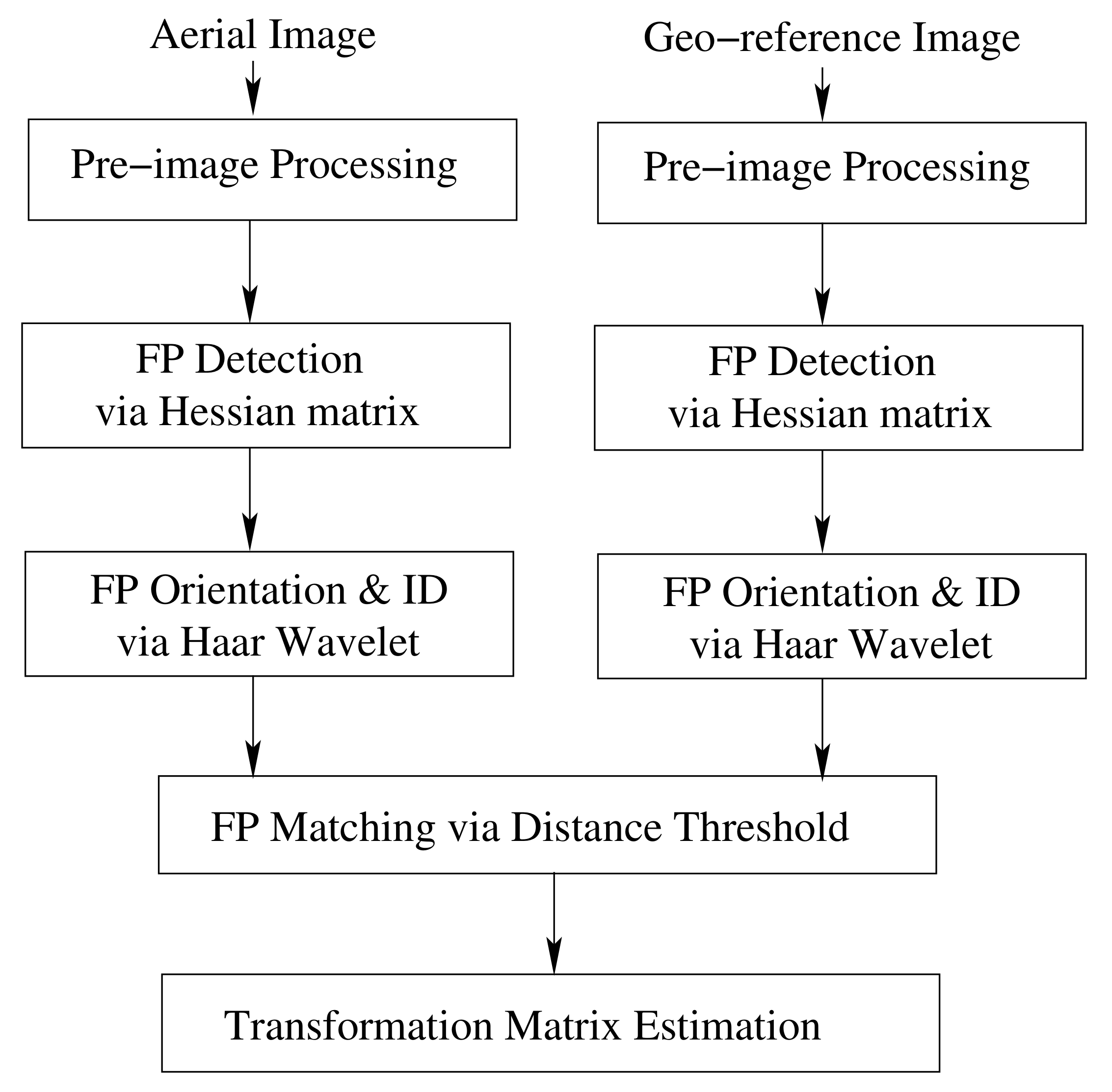
The SURF feature point detector adopts a Hessian matrix measure where the Laplacian of Gaussian is approximated by the difference of Gaussian. Similar to SIFT, SURF uses a local-based descriptor that describes a distribution of Haar wavelet responses in the neighbourhood of an interest point that is defined as a salient feature from a scale-invariant representation. However, the approximations and modifications made by the SURF method enable it to use the integral of images [19], which can be quickly computed independent of image size, to replace the majority of computations. We implemented a standard SURF algorithm for this work, as shown in Figure 2. The preimage processing includes grayscale filtering to mitigate lighting disturbance and image resizing to match the intrinsic properties of camera. The SURF algorithm runs autonomously in the proposed UAV self-localization system. As a compromise for performance and computational efficiency, we restrict the maximum number of feature points to 2000. Extra care is taken to terminate and thus exclude inconsistent registration processes. For example, we discard the outcome of an image registration if the number of matched feature points is less than four or the estimated transformation matrix is ill-conditioned.
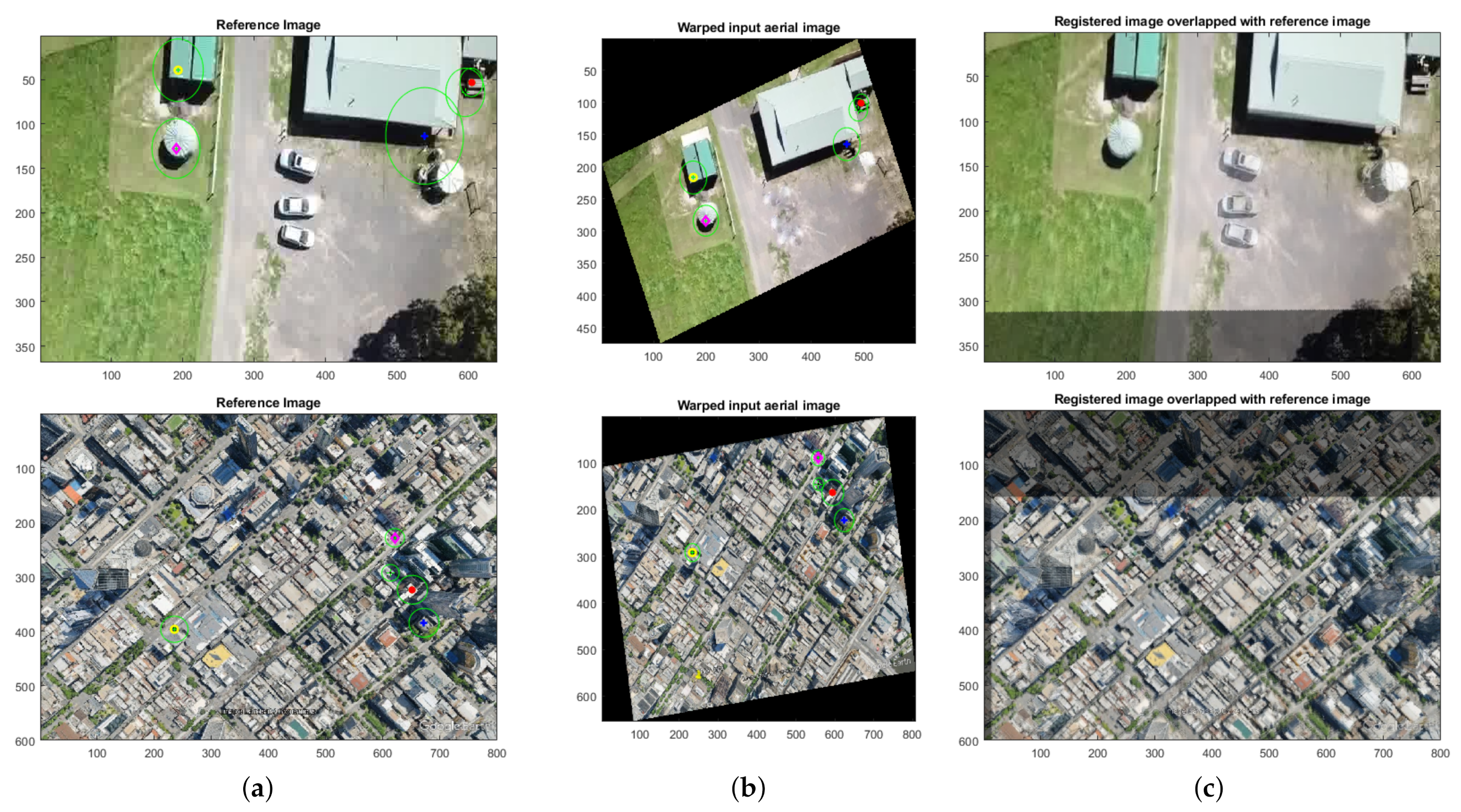
We present two image alignment examples in Figure 3 to demonstrate the robustness and effectiveness of the implemented algorithm. The scenes of UAV aerial images (middle column) are partially overlapped with that of reference images (left column) but with rotation and scale deformation. We also deliberately removed three white cars from the aerial image in the top row. In both cases, the first five significant feature points, which are marked in different colours, and their weights are correctly matched. Registration outcomes are shown in the right column on top of their reference images.
2.3. Registration Error Analysis
Monte Carlo simulation runs are carried out for testing the algorithm performance in terms of scale and rotation estimation errors. Two cases of aerial view were considered in the simulation, i.e., the scene of an aerial image may be overlapped with that of the reference image either partially or in full. At each run, an aerial image is obtained from warping the reference image and the rotation angle and scale factor , which are used for warping, are drawn from uniform distributions and , respectively. The choice of these parameter ranges in the simulation are based on the consideration that the registration algorithm is able to cover potential deformation uncertainties of the common scene between an aerial image and georeferenced image when the UAV is switched to localization mode near a georeferenced location. The results for two different image scene cases, averaged from 100 runs, are summarized in Table 1. These results demonstrate a low and consistent estimation error performed by the image registration algorithm with a great computational efficiency (CPU time is calculated on a HP Elitebook Intel(R) Core(TM) i7-7600U 2.8 GHz).
3. UAV Steering Controls Driven by Similarity Deformation
3.1. Transformation Matrix Estimation
Equation (1) may be written in the following form
where the transformation matrix
contains all deformation information between the image pair. In the localization mode of the proposed system, the parameters of , and and thus transformation matrix T, are estimated by the SURF algorithm. UAV steering controls are then generated from the values of the estimate transformation matrix . The generated controls aim to steer the UAV toward the scene of the georeferenced image such that the overlapping area between the aerial view of the UAV and georeferenced image increase and in the meantime the transformation matrix is updated by the registration from a new aerial view. This control process is expected to be progressively iterated until the estimated transformation matrix approach to an identity matrix.
3.2. Derivation of UAV Controls
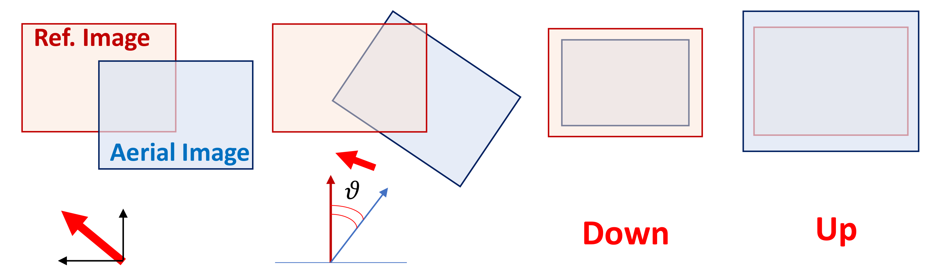
Under similarity mapping, we expect the UAV steering process to have controls of four degrees of freedom gained from the output of image registration. As illustrated in Figure 4, these controls are moving left or right, moving forward or backward, turning clockwise or counterclockwise, and flying up or down.
Table 2 lists the control types derived from the parameter values of the transformation matrix estimated by the image registration algorithm. When several controls are presented simultaneously, priority will be given to the correction of rotation, scale, and displacement, successively. The relation between control parameters in Table 2 and the estimated transformation matrix can be approximated as follows:
The derived controls are for driving a first-order feedback controller that steers the UAV to the direction that will minimize image registration error. They are implementable by many existing flight controllers, such as the PX4 autopilot platform [20].
The UAV self-localization process is an optimization procedure against a control cost and is performed iteratively in a feedback control loop. Upon receiving a control signal interpreted by the estimated transformation matrix, the UAV is steered to approach the scene of the reference image. Then, a new aerial frame is compared with the reference image to generate a new set of controls. Driven by these controls, the UAV gradually approaches the scene of the reference image. The process is repeated until control cost is no longer decreasing, or, in other words, the scene of aerial frame is completely overlapped with that of the reference image.
3.3. Control Cost
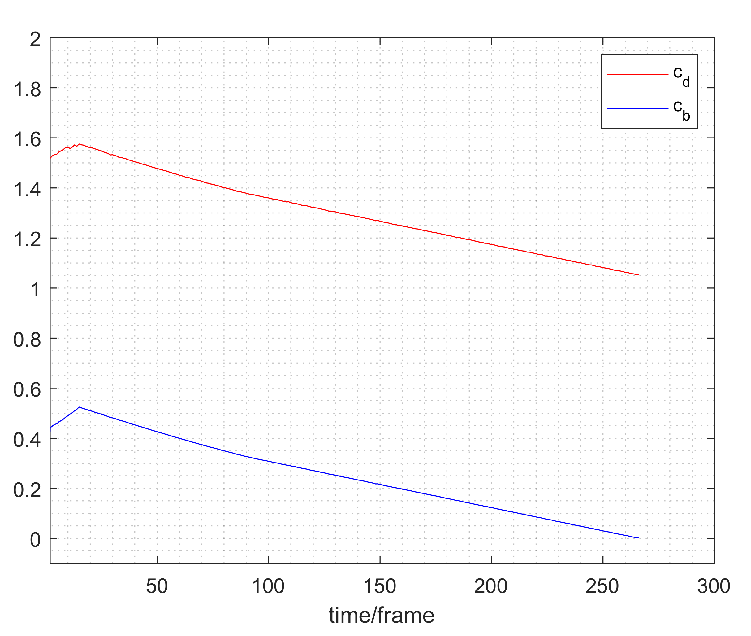
The choice of control cost criterion is crucial to the accuracy of the iterative image alignment process. In this work, UAV steering control will be permitted only if a suitable control criterion can be met. Essentially, we calculate two quantities from the estimated transformation matrix as the control cost. They are
- normalized displacement :where is the size of aerial (or georeferenced) image.
- determinant of transformation matrix :
As shown in Figure 5, the values of both cost functions are found to be monotonically decreasing as the UAV approaches the scene of the georeferenced image during UAV localization mode. Nevertheless, their turning points are sometimes slightly different, which may cause a larger location error if only using one of them. We therefore adopt both as the control cost, and a successful localization is claimed only if both have reached their turning points.
It is worth mentioning that to be more robust and accurate in practical applications, we may select the georeferenced images that have feature points that are as salient as possible and, with shadow and lighting directions, that are as consistent as possible with the actual environment.
4. Experiment and Results
In this work, we focus on the evaluation of the system in the form of Monte Carlo simulations, where the UAV camera is simulated and aerial images are taken from Google Earth Pro© in a virtual test environment. In this experiment, we aim to:
- provide a comprehensive understanding of the proposed system functionality, the way of the best functioning and additional control needed, etc.
- check the robustness of the proposed algorithm as well as potential localization strategies.
4.1. Simulation Scenario
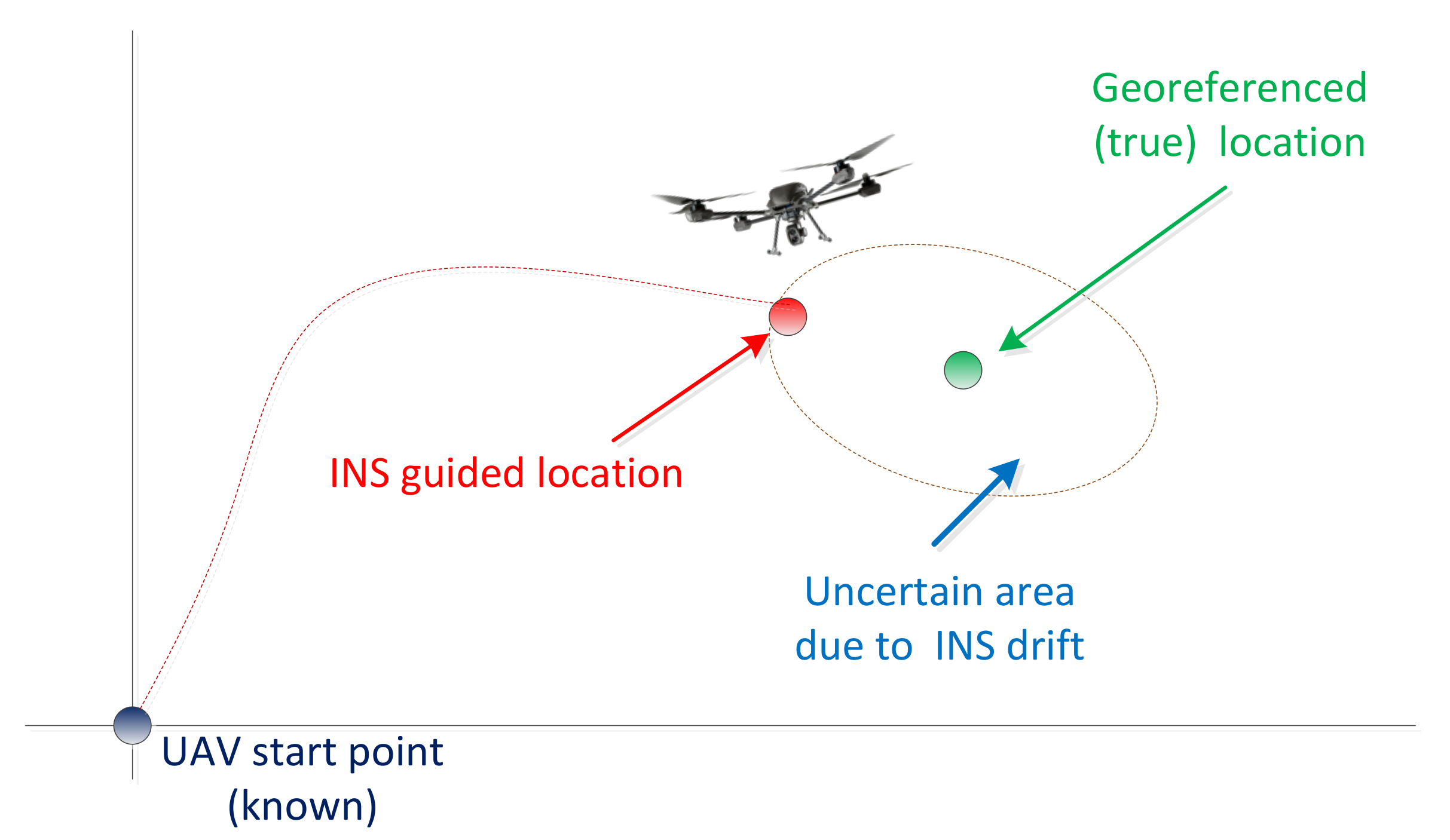
A flying UAV is guided by an inertial navigation system (INS) that calculates the UAV dead reckoning position and attitude from the observations of an onboard inertial measurement unit (IMU). Without an external aiding source, INS suffers from growing bias and drift over time, propagated from IMU errors. Typically, the INS integrates external location references, such as GNSS signal, via a Kalman filter [1]. In the proposed system, as show in Figure 6, we use aerial video to regularly obtain accurate location information as an alternative source of aiding in a GNSS-denied environment. We assume that aerial images taken by the aerial camera onboard the UAV are of the same optical properties (e.g., view angle, image size, etc.) as those of the georeferenced images. Otherwise, a proper image processing technique may be applied to retrieve the difference of the optical properties so that a consistent image registration can be performed. At each localization process, the UAV moves toward the area of the georeferenced image guided by onboard INS before the system is switched to localization mode. The UAV motion is then controlled by the image registration output until the scene of the onboard aerial camera is matched with that of the georeferenced image.
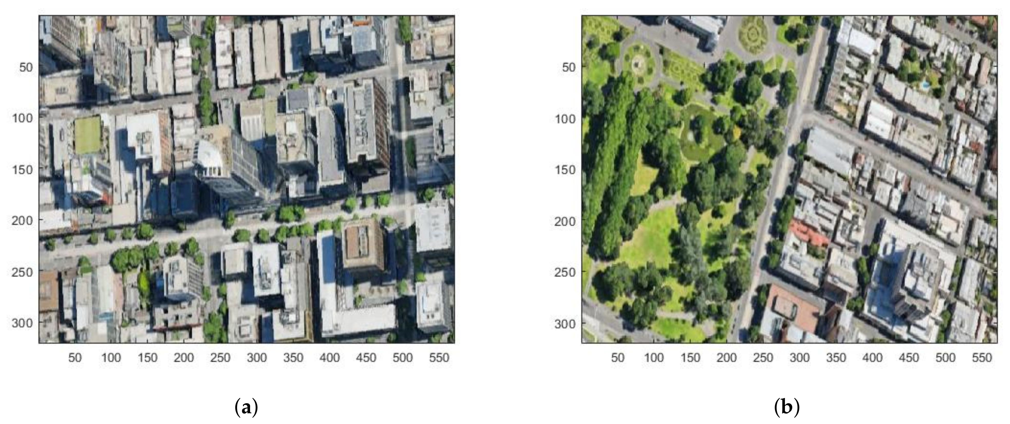
Figure 7 shows the entire scene of the UAV flying zone used in the simulation. It is a high-resolution image of size pixels and corresponds to approximately 0.87 m per pixel. In this image, we marked the UAV takeoff location using a red square and the georeferenced scene using a green circle, both of which are from a single realization of 100 Monte Carlo simulations. The corresponding aerial image at the UAV start location and georeferenced image are shown in Figure 8a,b, respectively.
In the Monte Carlo simulations, a virtual camera of resolution pixels is simulated to take aerial images from the flying UAV. We assume that both aerial and georeference image sizes are identical. In each run, the locations of both the UAV starting point and the scene of the geo-reference image are uniformly drawn from the full scene area. In each run, the UAV enters the scene of the georeferenced image navigated by the onboard INS. Bias and drifts of inertial sensors yield navigation error of INS. Here, this navigation error is defined by the distance between the center of the scene of the georeferenced image and the actual position that the UAV has reached, and it is modelled as a uniformly distributed random variable whose distribution is , where
The setup of (8) ensures that when the UAV switches into localization mode from INS navigation, a partially overlapped scene can be found from both the aerial and georeferenced images, which is a reasonable assumption in practice. In our experiment, and , the UAV will enter into localization mode at a “pixel distance” distribution in x direction and in y direction to the center of the scene of the georeferenced image at each run.
In the localization mode, the aerial images taken from UAV camera are compared with a georeferenced image and the cost is calculated based on the image registration output. In this experiment, when , it is found that at least three consecutive transformation matrices can be estimated consistently by image registration, and thus we let the UAV lock into localization iteration, where UAV controls are generated from every output of the image registration. The UAV is then steered by these controls and progressively approaches the scene of the georeferenced image. The localization process is completed if the stopping criterion described in Section 3.3 is met, that is, if the matching error (see Figure 5) is no longer decreasing. The proposed localization procedure is a trial-and-error process. The first attempt of the UAV self-localization starts from the INS-computed location (see Figure 6). In the case where has not fallen below 0.8 for a predefined short period, say, 10 sampling periods, another attempt of the UAV self-localization will be triggered and the UAV will be steered to a new starting location , where is drawn from a zero-mean Gaussian distribution with standard deviation described by nominal position error of INS. The system is designed to repeat this process until the UAV enters into the (locked-up) localization iteration and completes the localization process.
Figure 9 shows a snapshot of the experiment from a single run. In this example, the georeferenced image was taken from the point marked with a green circle and it was rotated clockwise. It was also enlarged by a scale factor of 1.46 as if it were taken from a lower altitude than that of the UAV actually flying. Furthermore, white noise of was added to the intensity of the georeferenced image. All of these added additional challenges to the UAV self-localization process.
4.2. Localization Error Analysis
Apart from randomly drawing the locations of the UAV starting point, the georeferenced scene, and the point at which the UAV enters into localization mode, we also warp the georeferenced image at each run to cover potential image variations caused by environment changes as follows:
- Assume a random angle between the directions of the UAV heading and georeferenced image scene. The angle distribution is of Gaussian zero-mean with a standard deviation .
- Assume that height at which the georeferenced image was taken is random such that the corresponding scale factor between the UAV aerial image and the georeferenced image follows from a uniform distribution .
- A white noise of is added to intensities of the georeferenced image.
As mentioned earlier, the full scene of the UAV flying area shown in Figure 7 is a high-resolution image of size pixels with a scale of 0.87 m per pixel. In the controller design, we allow the final scale accuracy , where is the estimated scale in (5) and is the true scale. Therefore, the actual distance resolution is meter per pixel.
From the matching error in (6), and assuming that the errors in x and x directions are of the same scale, we may roughly estimate the matching error bound in terms of distance as
For the current experiment setup, we have (m), where is the average cost at final localization iteration.
Table 3 lists statistical results obtained from 100 Monte Carlo runs for the proposed UAV self-localization process. In the experiment, the average UAV speed in INS navigation stage is 10 m/s and in the localization locked up (iteration) stage is 3 m/s.
As mentioned earlier, the localization iteration is a trial-and-error process. A single trial of localization process is deemed as an attempt. In 81 out of 100 runs, the UAV locks into localization iteration from INS navigation mode in the first attempt, and complete localization process successfully. The average time from the UAV taking off to the localization process completion is 72 s at a frame rate 5 frames per second. About 14% of the runs completed with two attempts, 4% with 3 attempts, and 1% with 4 attempts.
It is observed that the deformation level of reference image has a direct impact on the localization accuracy. The more attempts made for the UAV entering into the (locked-up) localization mode and thus completing the localization process, the larger the average localization error is. In those simulations in which more than one attempt have been made, the warp level of the georeferenced image is often more severe than average.
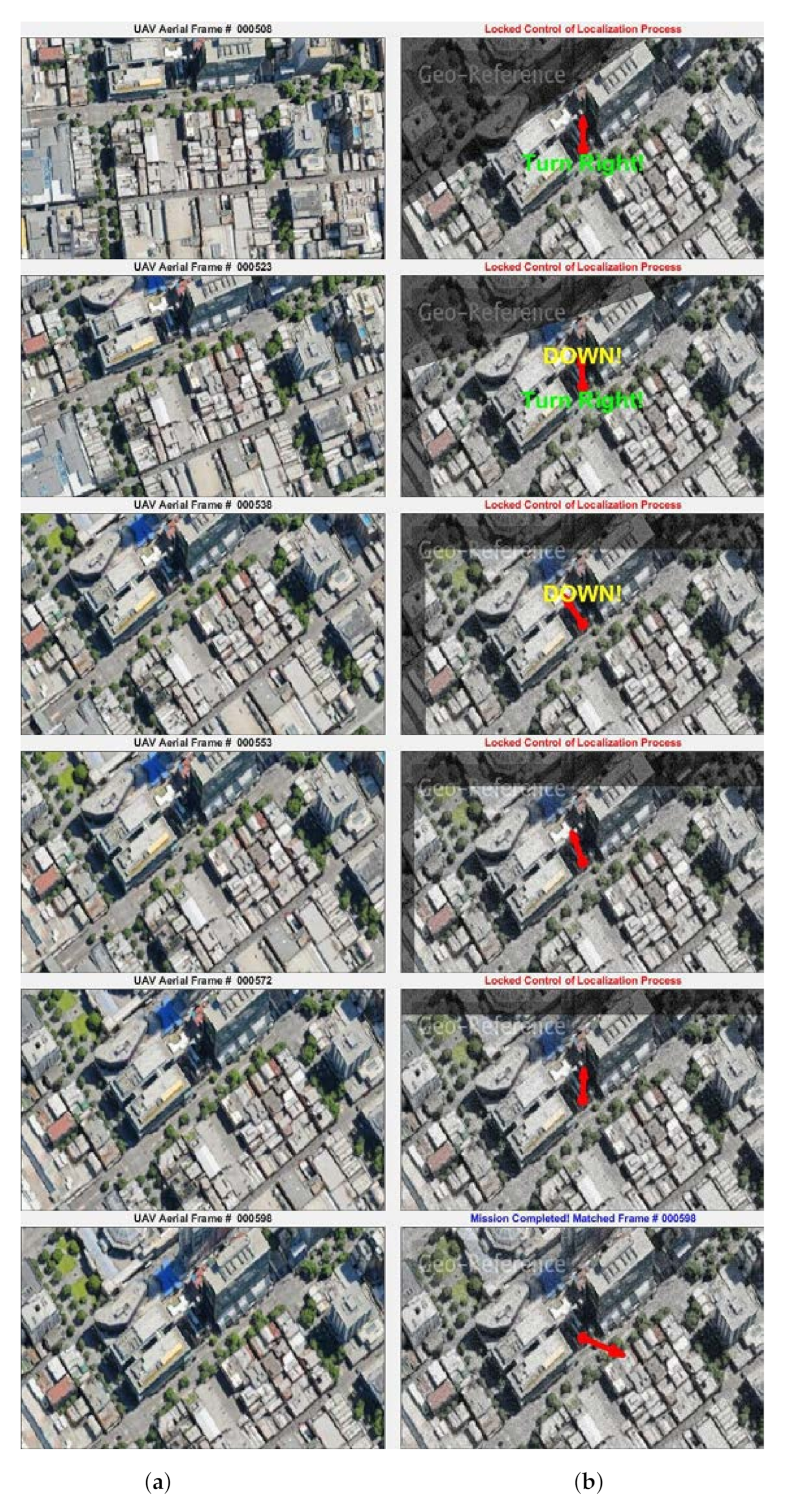
The UAV localization locked-up control process is demonstrated in Figure 10, which was recorded from a single run. The left column shows the aerial image sequence (along the time line from top to bottom) taken by the UAV during the process and the right column displays the sequence of registered images on top of the georeferenced image, where we also indicate the operation status of UAV controller (turn right, flying down, and moving direction, etc.). Although the entire locked-up control process takes up about 50 frames, only six frames are shown here to illustrate the process. In this particular example, the UAV motion is driven by controls generated by the registration algorithm involving right turn, flying down, moving left, and forward operations during the locked-up localization process.
We carried out 100 further Monte Carlo runs where the georeference images and UAV aerial images are taken at different times of the day. In each run, the georeferenced image is drawn from the full scene image taken at 4:30 p.m. in the afternoon, whereas the UAV localization is performed at 10 a.m. in the morning. As shown in Figure 11, this leads to the image pair to be registered with different lighting conditions caused by different sun illumination directions.
Similar to Table 3, we present the statistical results of the 100 Monte Carlo runs for image pairs with different lighting conditions in Table 4. While the localization process for all runs have successfully completed, the average time used is longer than those without lighting issues. The mean accuracy and localization error are slightly larger as well.
This reflects the fact that the difference of sun direction has considerable negative impact on the image registration algorithm. Overall, there is no localization failure case in our experiment. The proposed UAV localization system is therefore resilient against potential failure, showing a strong robustness and effectiveness, in particular, in the latter test results.
5. Conclusions
In this paper, the problem of autonomous UAV self-localization in a global-positioning-system (GPS)-denied environment is approached by comparing the aerial images taken by an onboard camera with a georeferenced image. A SURF feature-based image registration algorithm is designed and implemented. The algorithm is shown to be efficient and robust for real-time processing. Controls for UAV steering operation are derived from the image registration output based on the estimated similarity transformation matrix. We present a detailed statistical evaluation by Monte Carlo method in a simulated environment using Google Earth Pro©.
In the hardware development front, the proposed UAV self-localization system is being tested on a three-axis gimbal platform onboard a S500 drone in a controlled and laboratory environment as a proof of concept, where the aerial images are taken by a Pi camera module v2 and sent to a laptop computer via a WiFi communication channel. Image registration is performed remotely and generated UAV controls are then sent back to the flight controller (Pixhawk 4 mini autopilot via MAVlink) by WiFi link. We are implementing a Jeston-nano onboard processor to put all signal processing on the S500 platform. Consequent field test results will be published in future works.
Author Contributions
Conceptualization, X.W. and A.K.; methodology, X.W. and C.G.; software, X.W.; validation, X.W., W.L., B.J. and A.K.; formal analysis, X.W. and A.K.; investigation, X.W., A.K., W.L., B.J., C.G. and B.M.; resources X.W. and W.L.; writing—original draft preparation, X.W.; writing—review and editing, A.K. and S.L.M.; supervision, A.K.; project administration, A.K. and S.L.M.; funding acquisition, A.K. All authors have read and agreed to the published version of the manuscript.
Funding
This research received no external funding.
Conflicts of Interest
The authors declare no conflict of interest.
References
- Groves, P. Principles of GNSS, Inertial, and Multisensor Integrated Navigation Systems; Artech House: Norwood, MA, USA, 2013; pp. 419–448. [Google Scholar]
- Sanfourche, M.; Delaune, J.; Le Besnerais, G.; De Plinval, H.; Israel, J.; Cornic, P.; Treil, A.; Watanabe, Y.; Plyer, A. Perception for UAV: Vision-Based Navigation and Environment Modeling; Aerospace Laboratories: Bangalore, India, 2012. [Google Scholar]
- Achtelik, M.; Achtelik, M.; Weiss, S.; Siegwart, R. Onboard IMU and monocular vision based control for MAVs in unknown in- and outdoor environments. In Proceedings of the 2011 IEEE International Conference on Robotics and Automation, Shanghai, China, 9–11 May 2011. [Google Scholar] [CrossRef]
- Munguía, R.; Urzua, S.; Bolea, Y.; Grau, A. Vision-based SLAM system for unmanned aerial vehicles. Sensors 2016, 16, 372. [Google Scholar] [CrossRef] [PubMed]
- Balamurugan, G.; Valarmathi, J.; Naidu, V.P.S. Survey on UAV navigation in GPS denied environments. In Proceedings of the 2016 International Conference on Signal Processing, Communication, Power and Embedded System (SCOPES), Paralakhemundi, India, 3–5 October 2016. [Google Scholar] [CrossRef]
- Wang, X.; Moran, B.; Challa, S. Efficient Feature Aided Multi-object Tracking in Video Surveillance. In Proceedings of the 3rd International Conference on Image Processing and Signal Processing (CISP’10), Yantai, China, 16–18 October 2010; pp. 114–118. [Google Scholar]
- Xu, Y.; Pan, L.; Du, C.; Li, J.; Jing, N.; Wu, J. Vision-based UAVs Aerial Image Localization. In Proceedings of the 2nd ACM SIGSPATIAL International Workshop on AI for Geographic Knowledge Discovery, Seattle, WA, USA, 6 November 2018. [Google Scholar] [CrossRef]
- Luo, R.; Kay, M. Multisensor integration and fusion in intelligent systems. IEEE Trans. Syst. Man Cybern. 1989, 19, 901–931. [Google Scholar] [CrossRef]
- Lu, Y.; Xue, Z.; Xia, G.S.; Zhang, L. A survey on vision-based UAV navigation. Geo-Spat. Inf. Sci. 2018, 21, 21–32. [Google Scholar] [CrossRef]
- Conte, G.; Doherty, P. Vision-Based Unmanned Aerial Vehicle Navigation Using Geo-Referenced Information. EURASIP J. Adv. Signal Process. 2009, 2009, 387308. [Google Scholar] [CrossRef]
- Padró, J.C.; Muñoz, F.J.; Planas, J.; Pons, X. Comparison of four UAV georeferencing methods for environmental monitoring purposes focusing on the combined use with airborne and satellite remote sensing platforms. Int. J. Appl. Earth Obs. Geoinf. 2019, 75, 130–140. [Google Scholar] [CrossRef]
- Jin, Z.; Wang, X.; Moran, B.; Pan, Q.; Zhao, C. Multi-region scene matching based localisation for autonomous vision navigation of UAVs. J. Navig. 2016, 69, 1215–1233. [Google Scholar] [CrossRef]
- Brown, L.G. A survey of image registration techniques. ACM Comput. Surv. 1992, 24, 325–376. [Google Scholar] [CrossRef]
- Evangelidis, G.D.; Psarakis, E.Z. Parametric Image Alignment Using Enhanced Correlation Coefficient Maximization. IEEE Trans. Pattern Anal. Mach. Intell. 2008, 30, 1858–1865. [Google Scholar] [CrossRef] [PubMed]
- Guizar-Sicairos, M.; Thurman, S.T.; Fienup, J.R. Efficient subpixel image registration algorithms. Opt. Lett. 2008, 33, 156–158. [Google Scholar] [CrossRef] [PubMed]
- Zhang, X.; Gilliam, C.; Blu, T. All-Pass Parametric Image Registration. IEEE Trans. Image Process. 2020, 29, 5625–5640. [Google Scholar] [CrossRef] [PubMed]
- Lowe, D. Object recognition from local scale-invariant features. In Proceedings of the Seventh IEEE International Conference on Computer Vision, Kerkyra, Greece, 20–27 September 1999. [Google Scholar] [CrossRef]
- Bay, H.; Tuytelaars, T.; Gool, L.V. SURF: Speeded Up Robust Features. In Computer Vision—ECCV 2006; Springer: Berlin/Heidelberg, Germany, 2006; pp. 404–417. [Google Scholar] [CrossRef]
- Viola, P.; Jones, M. Rapid object detection using a boosted cascade of simple features. In Proceedings of the 2001 IEEE Computer Society Conference on Computer Vision and Pattern Recognition, Kauai, HI, USA, 8–14 December 2001; Volume 1. [Google Scholar]
- Dronecode, O.S. PX4 Autopilot User Guide; UAV Controller Platform: Wichita, Kansas, 2020. [Google Scholar]
Figure 1.
Illustration of the unmanned aerial vehicle (UAV) self-localization process using landmark images.
Figure 1.
Illustration of the unmanned aerial vehicle (UAV) self-localization process using landmark images.

Figure 2.
Flowchart of the implemented speeded-up-robust-features (SURF)-based algorithm. The algorithm outputs estimated transformation matrix by solving (2) using feature point pairs if more than four matched feature points (FP) between image pair are found.
Figure 2.
Flowchart of the implemented speeded-up-robust-features (SURF)-based algorithm. The algorithm outputs estimated transformation matrix by solving (2) using feature point pairs if more than four matched feature points (FP) between image pair are found.

Figure 3.
Performance of the registration algorithm implemented in this work. Column (a): reference images. Column (b): Aerial images taken by UAV whose scenes are partially identical to those of reference images. Column (c): registration results, where the registered images are on top of the corresponding reference images. The first five significant feature points, which can be distinguished by colour, are marked in both the reference images (a) and aerial images (b).

Figure 4.
Illustration of UAV steering control from image registration outcomes under similarity transformation. From left to right images: the UAV steering control due to partial scene overlapping, rotation, scale less than unit, and scale greater than unit with respect to the georeferenced image.
Figure 4.
Illustration of UAV steering control from image registration outcomes under similarity transformation. From left to right images: the UAV steering control due to partial scene overlapping, rotation, scale less than unit, and scale greater than unit with respect to the georeferenced image.

Figure 5.
Typical values of the cost function in the locked-up localization process.

Figure 6.
Illustration of the UAV inertial navigation strategy aided by the proposed aerial image registration system. The UAV starts from a known point and is guided by the intertial navigation system (INS) to the INS-computed georeference location (red dot). The green dot signifies the true georeferenced location. The UAV steered from the INS-computed georeferenced location to the true georeferenced location via the image registration system.

Figure 7.
Entire UAV flying zone for simulation generated using Google Earth Pro. The red square is the UAV takeoff location and the green circle is the location where the reference image is taken.
Figure 7.
Entire UAV flying zone for simulation generated using Google Earth Pro. The red square is the UAV takeoff location and the green circle is the location where the reference image is taken.

Figure 8.
(a) UAV aerial image taken at the UAV starting location (red square). (b) Georeferenced image taken at the location of the green circle in Figure 7.
Figure 8.
(a) UAV aerial image taken at the UAV starting location (red square). (b) Georeferenced image taken at the location of the green circle in Figure 7.

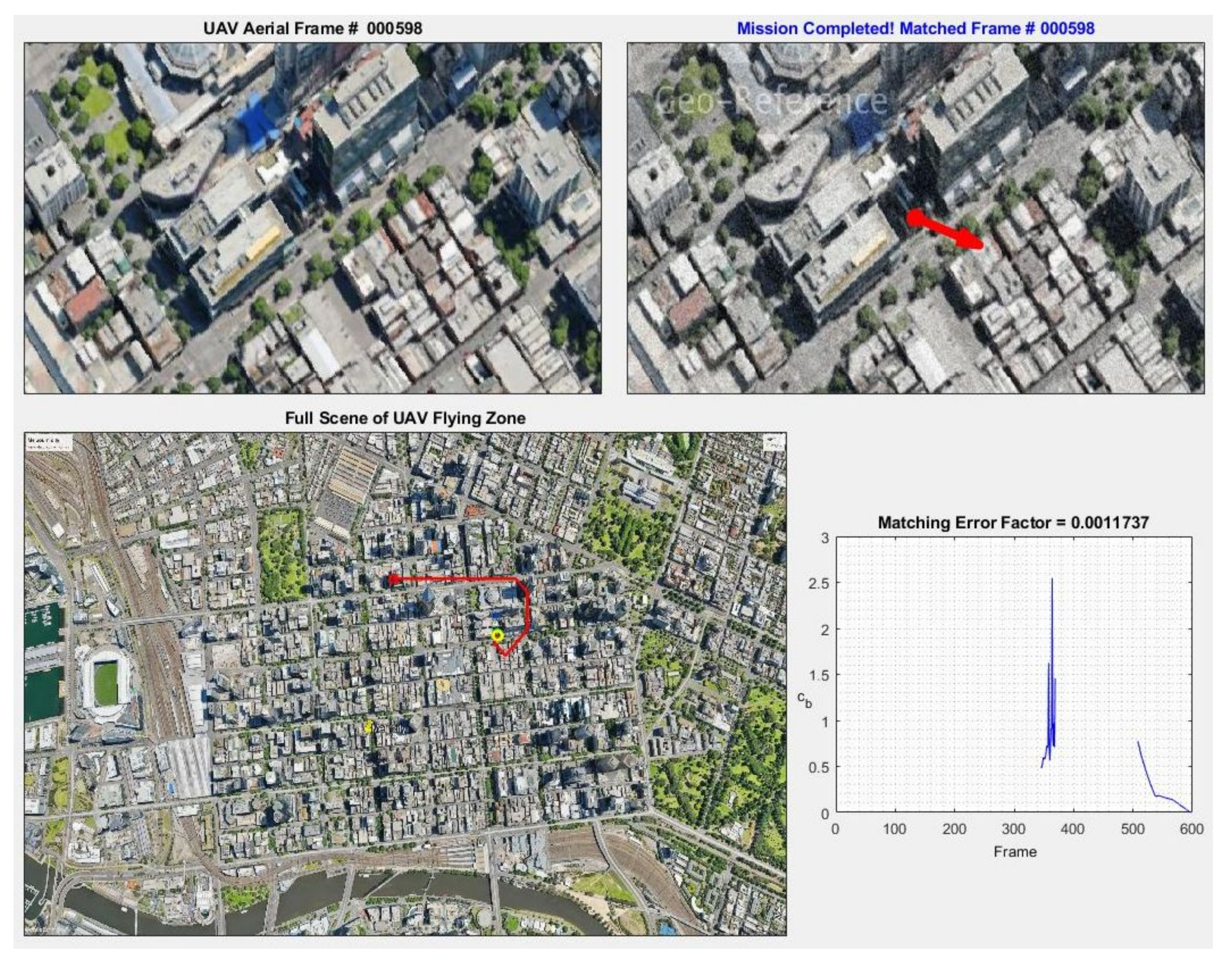
Figure 9.
The top left is the UAV aerial camera view window. The top right displays the process of UAV localization when the image registration algorithm captures the scene of reference image. The bottom left is the full view of UAV flying zone image, where the green circle is the location where the reference image was taken, the red square is the UAV takeoff location and the yellow circle represents the flying UAV with its trajectory highlighted by a red curve. The right lower corner window plot the normalized matching accuracy when the UAV enters into localization mode. The discontinuity of curve signifies that this particular localization process experienced two attempts.

Figure 10.
Illustration of a typical UAV locked-up localization process that involves all UAV controls generated by image registration as discussed in Section 3. The entire process takes up about 50 frames. We only show six of those frames. Column (a): UAV aerial camera view. Column (b): aerial images “registered” on top of georeferenced image. For this particular example, the localization accuracy is within 3 m. The processing frame rate is 5 fps (Intel(R) Core(TM) i7-7600U).

Figure 11.
Illustration of image difference due to different sun illumination directions. (a) Aerial image taken at 10 a.m. in the morning. (b) Georeferenced image taken at 4:30 p.m. in the afternoon.
Figure 11.
Illustration of image difference due to different sun illumination directions. (a) Aerial image taken at 10 a.m. in the morning. (b) Georeferenced image taken at 4:30 p.m. in the afternoon.


Table 1.
Statistical error performance from 100 Monte Carlo runs, where all errors are root mean square errors.
Table 1.
Statistical error performance from 100 Monte Carlo runs, where all errors are root mean square errors.
| Image Size | Scene Type | Scale Error | Rotation Error | CPU (s) |
|---|---|---|---|---|
| 600 × 800 | Partial | 0.015 | 0.024° | 0.59 |
| 368 × 640 | Partial | 0.01 | 0.02° | 0.09 |
| 368 × 640 | Full | 0.015 | 0.013° | 0.1 |
| 600 × 800 | Full | 0.0014 | 0.0014° | 0.49 |
Table 2.
First-order UAV control signal generation.
| Parameter | Value | UAV Control | Process Order |
|---|---|---|---|
| Turn counterclockwise | 1 | ||
| Turn clockwise | |||
| a | Up | 2 | |
| Down | |||
| Left | 3 | ||
| Right | |||
| Forward | 3 | ||
| Backward |
Table 3.
Statistical results of Monte Carlo 100 runs.
| 1 Attempt | 2 Attempts | 3 Attempts | ≥4 Attempts | |
|---|---|---|---|---|
| Proportion | 81% | 14% | 4% | 1% |
| Mean # of frames | 346.7 | 531.1 | 773.5 | 720 |
| Average time (s) | 72 | 99.7 | 112.6 | 94.9 |
| Mean accuracy | 0.0041 | 0.0077 | 0.0064 | 0.0073 |
| (m) | ≤1.6 | ≤3 | ≤2.5 | ≤2.85 |
Table 4.
Statistical results of 100 Monte Carlo runs, where aerial image and reference image are with different sun illumination directions.
Table 4.
Statistical results of 100 Monte Carlo runs, where aerial image and reference image are with different sun illumination directions.
| 1 Attempt | 2 Attempts | 3 Attempts | ≥4 Attempts | |
|---|---|---|---|---|
| Proportion | 86% | 9% | 2% | 3% |
| Mean # of frames | 297 | 535 | 472 | 889 |
| Average time (s) | 82 | 141 | 135 | 225 |
| Mean accuracy | 0.0069 | 0.0106 | 0.005 | 0.0135 |
| (m) | ≤2.1 | ≤3.23 | ≤1.53 | ≤4.12 |
Publisher’s Note: MDPI stays neutral with regard to jurisdictional claims in published maps and institutional affiliations. |
© 2021 by the authors. Licensee MDPI, Basel, Switzerland. This article is an open access article distributed under the terms and conditions of the Creative Commons Attribution (CC BY) license (http://creativecommons.org/licenses/by/4.0/).
Share and Cite
MDPI and ACS Style
Wang, X.; Kealy, A.; Li, W.; Jelfs, B.; Gilliam, C.; Le May, S.; Moran, B. Toward Autonomous UAV Localization via Aerial Image Registration. Electronics 2021, 10, 435. https://doi.org/10.3390/electronics10040435
AMA Style
Wang X, Kealy A, Li W, Jelfs B, Gilliam C, Le May S, Moran B. Toward Autonomous UAV Localization via Aerial Image Registration. Electronics. 2021; 10(4):435. https://doi.org/10.3390/electronics10040435
Chicago/Turabian StyleWang, Xuezhi, Allison Kealy, Wenchao Li, Beth Jelfs, Christopher Gilliam, Samantha Le May, and Bill Moran. 2021. "Toward Autonomous UAV Localization via Aerial Image Registration" Electronics 10, no. 4: 435. https://doi.org/10.3390/electronics10040435
Note that from the first issue of 2016, this journal uses article numbers instead of page numbers. See further details here.