Article

Semi-Supervised Extreme Learning Machine Channel Estimator and Equalizer for Vehicle to Vehicle Communications

1
Department of Electrical Engineering, Universidad de Chile, Santiago 8370451, Chile
2
Centro de Investigación de Estudios Avanzados del Maule (CIEAM), Vicerrectoría de Investigación y Postgrado, Universidad Católica del Maule, Talca 3466706, Chile
3
Department of Computer Science and Industry, Faculty of Engineering Science, Universidad Católica del Maule, Talca 3480112, Chile
4
Department of Electrical Engineering, University of Santiago de Chile, Santiago 91701234, Chile
*
Author to whom correspondence should be addressed.
Electronics 2021, 10(8), 968; https://doi.org/10.3390/electronics10080968
Submission received: 12 February 2021 / Revised: 3 April 2021 / Accepted: 9 April 2021 / Published: 19 April 2021
(This article belongs to the Section Microwave and Wireless Communications)

Abstract

:
Wireless vehicular communications are a promising technology. Most applications related to vehicular communications aim to improve road safety and have special requirements concerning latency and reliability. The traditional channel estimation techniques used in the IEEE 802.11 standard do not properly perform over vehicular channels. This is because vehicular communications are subject to non-stationary, time-varying, frequency-selective wireless channels. Therefore, the main goal of this work is the introduction of a new channel estimation and equalization technique based on a Semi-supervised Extreme Learning Machine (SS-ELM) in order to address the harsh characteristics of the vehicular channel and improve the performance of the communication link. The performance of the proposed technique is compared with traditional estimators, as well as state-of-the-art machine-learning-based algorithms over an urban scenario setup in terms of bit error rate. The proposed SS-ELM scheme outperformed the extreme learning machine and the fully complex extreme learning machine algorithms for the evaluated scenarios. Compared to traditional techniques, the proposed SS-ELM scheme has a very similar performance. It is also observed that, although the SS-ELM scheme requires the largest operation time among the evaluated techniques, its execution time is still far away from the latency requirements specified by the standard for safety applications.

1. Introduction

Vehicular communications are a promising technology for deploying next-generation intelligent transportation systems [1,2]. Vehicular Communication Systems (VCSs) rely on Vehicle-to-Vehicle (V2V) and Vehicle-to-Infrastructure (V2I) communications subject to a time-varying, frequency-selective wireless channel for enabling road safety and traffic efficiency applications. Important efforts are being made towards the identification, definition, and characterization of applications and use cases for VCSs. For instance, the European Telecommunication Standards Institute (ETSI) has defined a basic set of vehicular applications to be considered as a reference for deployment and standardization [3]. ETSI has also specified the operation mode and communication requirements of vehicular applications, such as pre-crash sensing, lane change warning, and cooperative forward-collision warning [4,5]. These safety applications aim to decrease the probability of an accident by using early warnings, or even by taking control of the vehicle. On the contrary, vehicular applications such as adaptive cruise control and intersection management aim to decrease road congestion and improve traffic efficiency [3]. A challenge in VCSs is in satisfying the strict communication requirements of safety applications, which are vital for preserving human lives. Road safety applications have specified requirements concerning reliability and latency [4,5]; therefore, it is necessary for the the underlying structure of the vehicle network to guarantee these standards.
In VCSs, the particular propagation conditions of the vehicular environment make channel estimation and equalization a relevant challenge, especially because the high velocity of vehicles leads to variations in time and frequency [6]. In order to adapt to the harsh vehicular channel, the effective data rates of the IEEE 802.11p amendment were reduced to half in comparison to IEEE 802.11-based standards [7]. Traditional IEEE 802.11-based standards are the basis of Wireless Fidelity (WiFi) systems, which are commonly used in indoor scenarios and characterized by their low mobility [6,7]. Despite the particular propagation conditions of the vehicular environment and the high mobility of the vehicles, no modifications were made to the IEEE 802.11p amendment regarding the channel estimation techniques adopted by traditional IEEE 802.11-based standards. A well-known channel estimation technique is the Least Squares (LS), which estimates the impulse response of the channel at the start of a frame [8]. LS works well for typical indoor Orthogonal Frequency Division Multiplexing (OFDM) systems; however, its performance is degraded in vehicular environments because the channel changes rapidly over time, which is more critical for higher velocities [6]. Another channel estimation technique corresponds to the Spectral Temporal Averaging (STA) [9], which uses time and frequency dependencies to properly perform the estimation stage. STA unfortunately suffers a great performance impact in non Wide-Sense Stationary Uncorrelated Scattering (WSSUS) channels. Unlike STA, the Constructed Data Pilots (CDP) technique [8] does not suffer significant performance degradation on non-WSSUS channels, but it has poor performance at low Signal to Noise Ratios (SNRs).
Machine Learning (ML) provides a versatile set of tools to address the challenges of vehicular communications due to its ability to exploit available data and perform difficult tasks; for example, to predict channel parameters, to augment network throughput, and to help with congestion control or even autonomous driving [10]. There are several proposals [11,12,13] that use ML schemes to perform channel estimation and equalization, but these proposals do not consider the 802.11p amendment. In other words, these studies can not be extrapolated for VCSs because they do not consider the characteristics of the non-WSSUS mobile-to-mobile channel or the particular frame structure of the communication packet; therefore, the channel estimation must be performed differently to the 802.11p amendment mandates. In [11], Ye and Li used a Deep Learning (DL) approach characterized by off-line training to perform channel equalization and estimation for an OFDM-based system, by showing a performance improvement over the LS and the Minimum Mean-Square Error (MMSE) schemes. The work presented in [11] shows that DL has the potential to improve the estimation equalization of communication channel in OFDM-based schemes. However, when considering that V2V safety applications have latency limitations, and since the channel has rapid variations in the time and frequency domain, an off-line approach should be discarded, as the channel models used in the training stage might differ from the actual channel. In [12], Sattiraju et al. proposed an artificial neural network (ANN) scheme based on a convolutional neural network to perform channel estimation on a Cellular Vehicle-to-Everything (C-V2X) communication system. This technique performs well but it again requires an off-line learning stage. In [13], Liu et al. introduces the use of a fully Complex Extreme Learning Machine (C-ELM) neural network to perform channel estimation and equalization on OFDM signals, where an exponential channel model with eight stochastic fading delay paths based on the IEEE 802.11g standard (mainly, a frequency-selective channel) is considered. The results show that the proposed C-ELM algorithm outperforms other state-of-the-art techniques, such as MMSE, LS, and a deep neural network-based scheme, and has a better generalization ability by considering different subcarrier modulation formats and numbers of subcarriers. It is worth noting that only the hyper-parameters (mapping function and number of hidden neurons) of the C-ELM are reported; no theoretical or simulation justifications are presented.
In this work, as an initial exploration, we propose the use of an Extreme Learning Machine (ELM) channel estimator and equalizer technique, which is characterized by Semi-Supervised (SS) learning for vehicular communications. The proposed algorithm considers the special propagation conditions in the time and frequency domains of vehicular communication channels. The main contributions of this work can be summarized as follows:
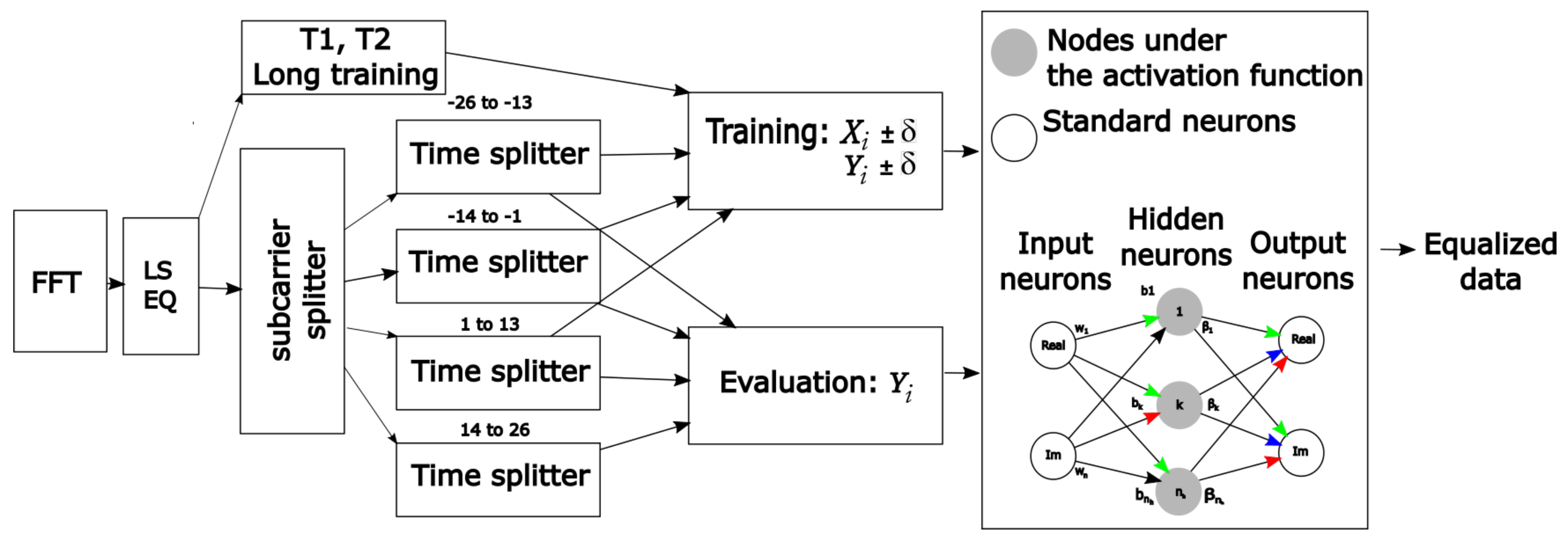
  • We propose a regularized ELM subject to SS learning as channel estimator and equalizer to enhance the performance of a representative IEEE 802.11p OFDM-based system in terms of Bit Error Rate (BER). To this end, we add a novel parameter denoted by δ in the Semi-supervised Extreme Learning Machine (SS-ELM) to address the time-domain fluctuations of the channel. Furthermore, a frequency-domain localized mapping is used to properly recover the OFDM signal, namely to address the frequency-selective channel;
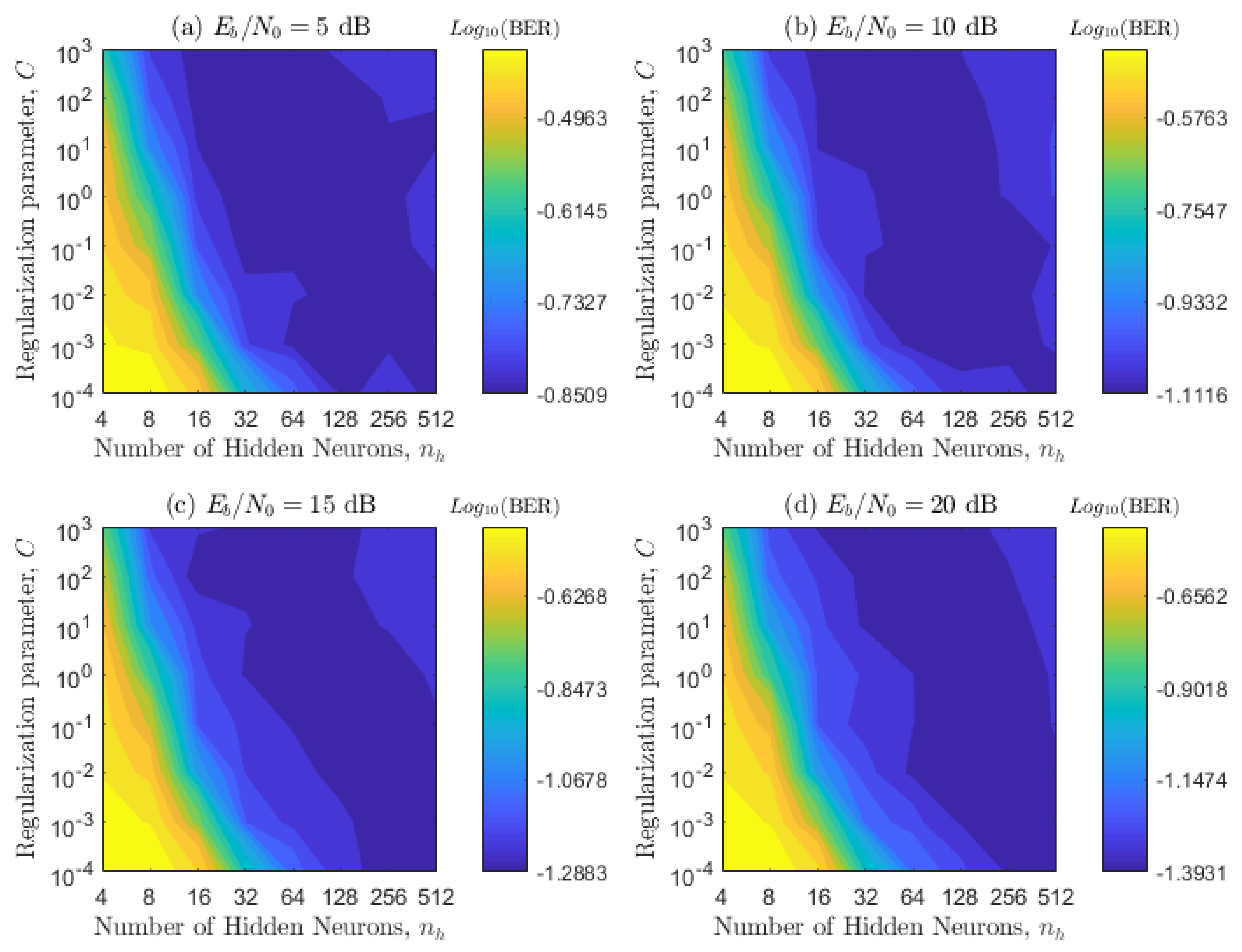
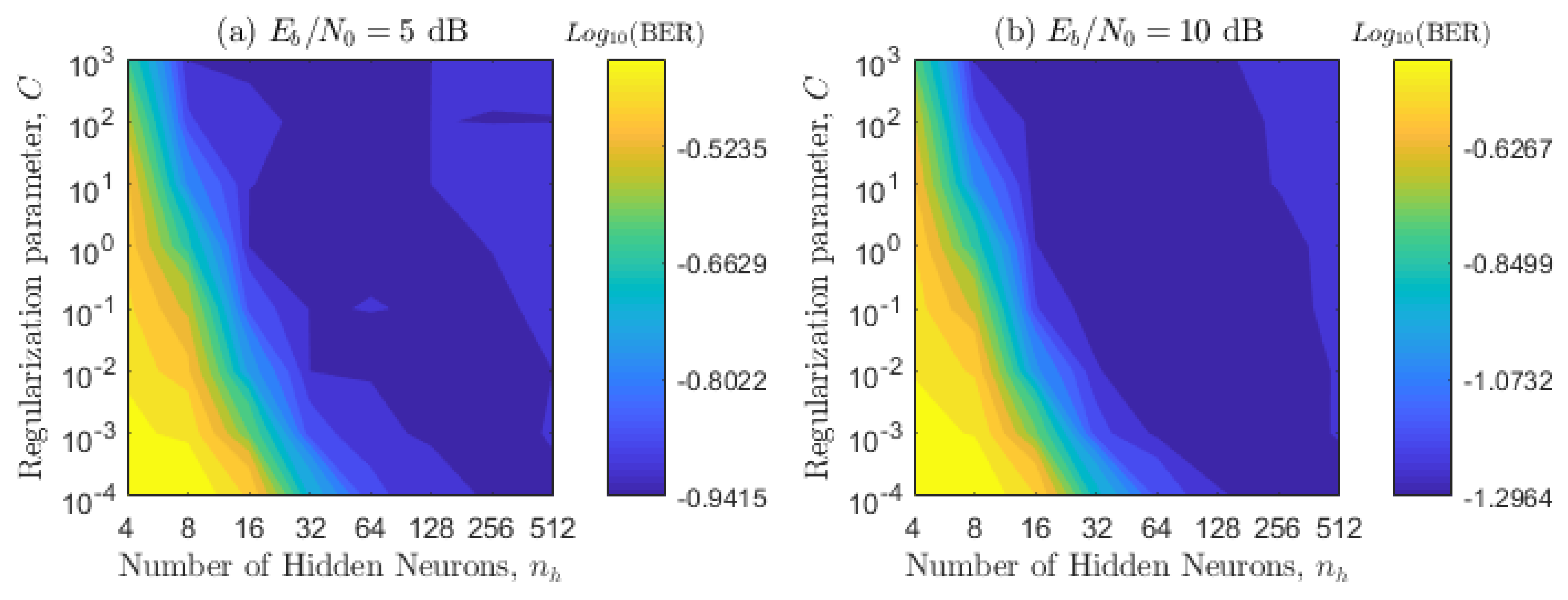
  • Taking the simulation framework of the evaluated system into account, we compute the sub-optimal SS-ELM hyper-parameters to diminish BER via extensive simulations. We also show that a supervised ELM does not improve the BER performance of a vehicular IEEE 802.11p system;
  • We compare the proposed technique with current state-of-the-art machine-learning-based channel estimation schemes as well as traditional techniques in an urban environment for several values of Energy per Bit to Noise Power Spectral Density Ratios ( E b / N 0 ). The addressed techniques are also contrasted in terms of the required processing time.
The remainder of this article is organized as follows: Section 2 depicts the foundations and background of this work, namely the physical layer of the IEEE 802.11p amendment, details of the vehicular channel model used in this work, and the ELM neural network subject to supervised and SS learning. Section 3 carefully presents the novel and improved SS-ELM algorithm used to estimate and equalize the communication channel of an IEEE 802.11p-based V2V system. Section 4 depicts the evaluation scenario, describes the optimization process of the SS-ELM parameters, and compares the BER and execution time of the proposed scheme with other state-of-the art and traditional IEEE 802.11 channel estimation techniques. Finally, Section 5 contains concluding remarks.

2. Background

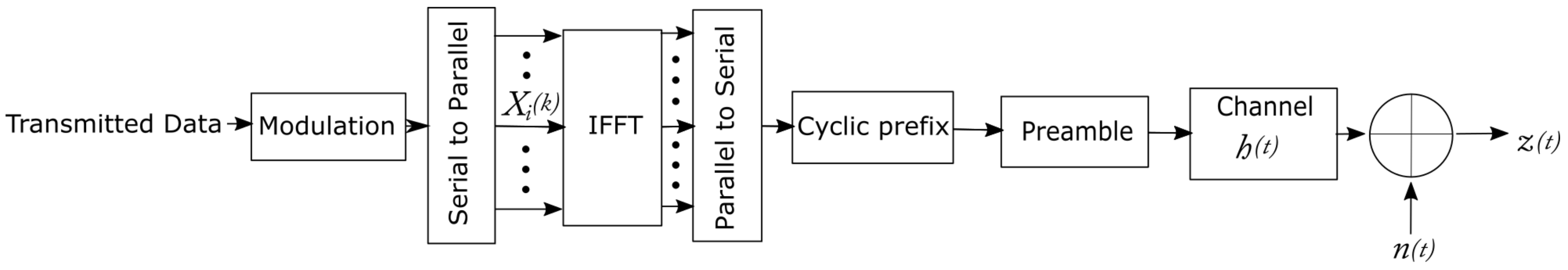
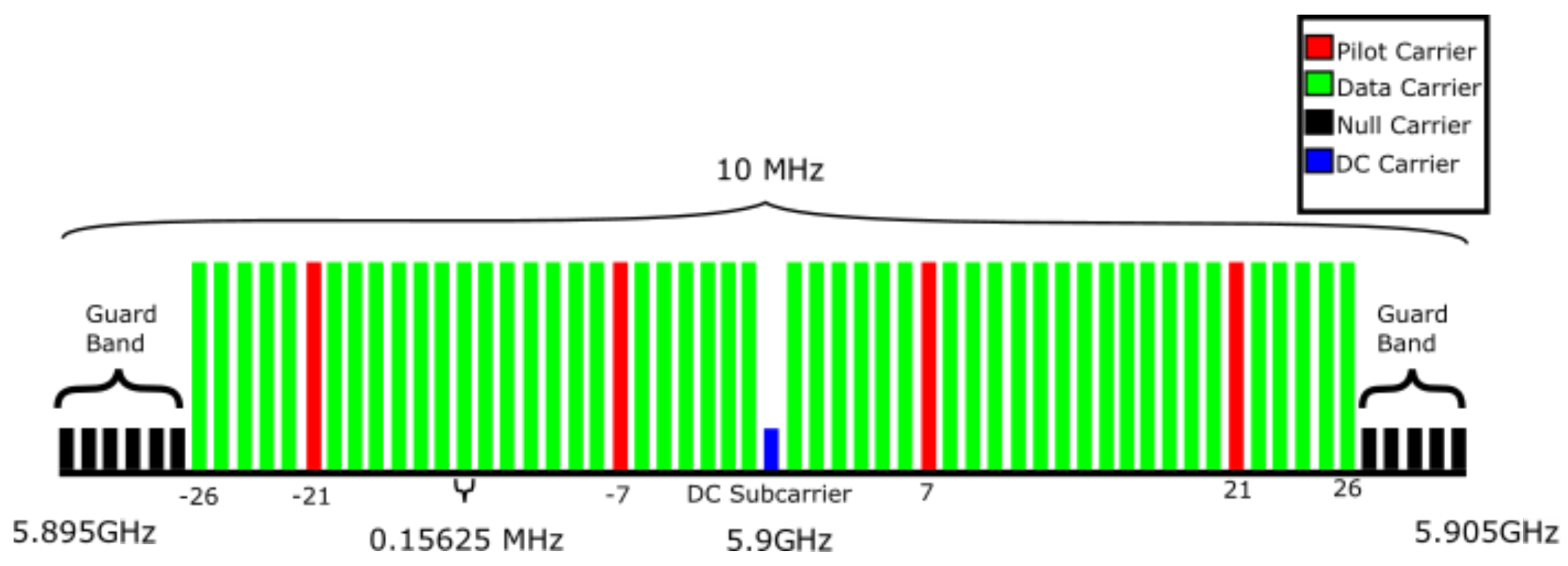
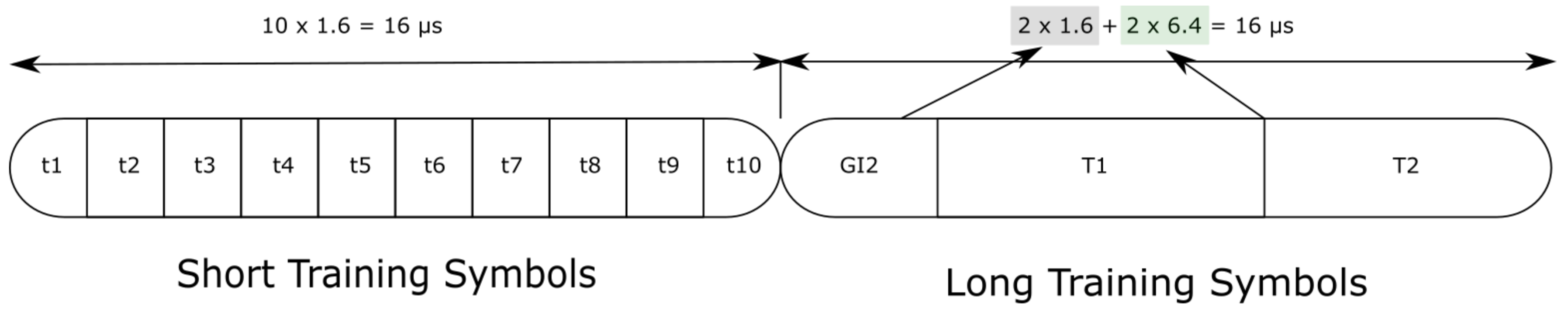
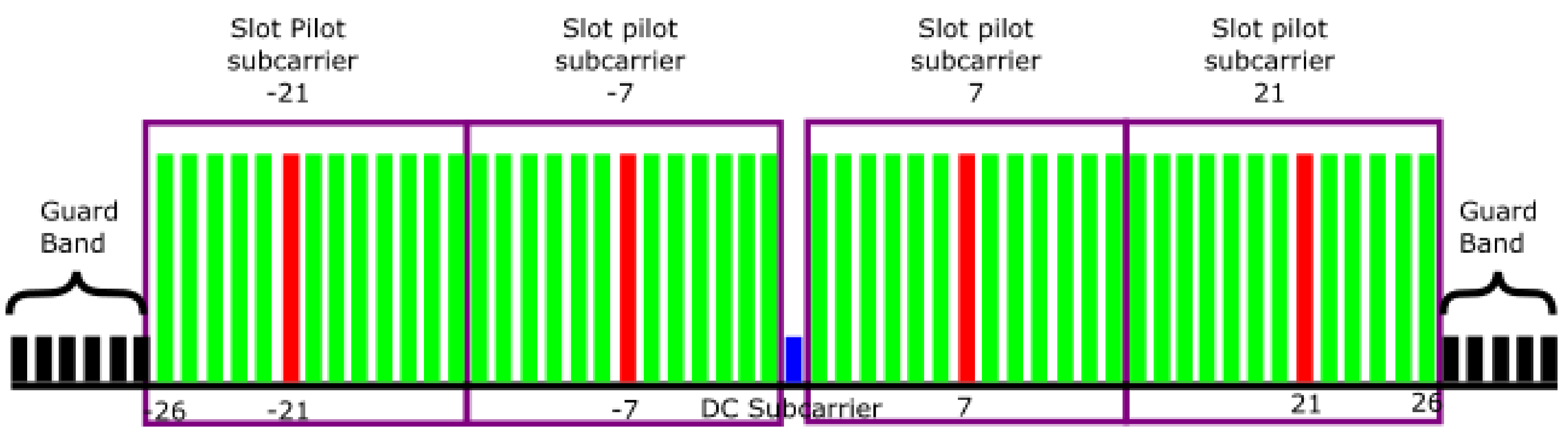
2.1. The IEEE 802.11p Standard

IEEE 802.11p is an amendment of the IEEE 802.11a standard [7]. Its purpose is to adapt existing indoor wireless communication systems to vehicular environments, where it is important to address the high mobility of the users. IEEE 802.11p uses OFDM as modulation format in the Physical Layer (PHY) and it operates at the 5.9 GHz radio frequency band. The transmitter sends several parallel data streams through orthogonal subcarriers, by improving the spectral efficiency and mitigating the severity of multi-path fading [7].
Table 1 shows the most important parameters defined on the IEEE 802.11p amendment. In general, the time domain parameters of this amendment are two times larger with respect to the IEEE 802.11a standard. For instance, the bandwidth is reduced from 20 MHz to 10 MHz, and the subcarrier frequency spacing is reduced by a factor of 2. As mentioned, these changes are made in order to increase the reliability of the transmission by increasing the duration of the OFDM symbols.
Figure 1 and Figure 2 depict a general IEEE 802.11p transceiver. The transceiver is based on traditional OFDM architectures. For simplicity, the block diagrams of the transceiver are depicted in its base-band representation. At the transmitter side, the data are modulated and then passed through an Inverse Fast Fourier Transform (IFFT) block to get orthogonal signals. Afterwards, a Cyclic Prefix (CP) is added to diminish inter-symbol interference, and finally a temporal preamble is inserted [7]. The purpose of this preamble is to synchronize the signal (short training symbols) and estimate the channel (long training symbols). Nevertheless, the structure of the preamble is detailed at the end of this Subsection. Figure 2 shows that the transmitted signal is distorted by the wireless channel, which is time-varying and frequency-selective for V2V communications (refer to the next Section), and by Gaussian additive noise, which is typical to all communication system. At the receiver side, the first signal processing task consists of removing the CP, and then applying a Fast Fourier Transform (FFT) to the signal. Then, the channel is estimated, and the signal is equalized by exploiting the subcarriers used as pilot signals. Finally, the signal is demodulated, and the data can be recovered.
The signal received after the FFT operation is given as follows [6]
Y i ( k ) = H i ( k ) X i ( k ) + N i ( k ) , i = { 1 , . . . , N s y m b o l } , k = { 1 , . . . , M } ,
where i corresponds to the respective OFDM symbol, N s y m b o l denotes the total number of OFDM symbols, k is the corresponding subcarrier, and M represents the total number of subcarriers. Furthermore, X i ( k ) represents the transmitted signal that is obtained after the modulation in the transmitter block diagram, Y i ( k ) is the received signal after the FFT module at the receiver side, H i ( k ) is the Channel Frequency Response (CFR), and N i ( k ) is the Additive White Gaussian Noise (AWGN).
Based on [6], Figure 3 depicts the subcarrier distribution of the IEEE 802.11p standard. As mentioned previously, the bandwidth of the OFDM signal is given by 10 MHz and the radio frequency matches to 5.9 GHz. The data subcarriers are shown in green, while the pilots are shown in red and are uniformly distributed between the data subcarriers. Additionally, the null and Direct Current (DC) subcarriers are represented by black and blue colors, respectively. For the sake of simplicity, in our work, null and DC subcarriers are discarded.
In Figure 4, the IEEE 802.11p packet preamble structure is illustrated. It can be seen that the preamble has 10 short training symbols of 1.6 µs located at the beginning of the packet. These symbols are used to perform fine synchronization. In this work, the use of these symbols is discarded, since we assume a perfect synchronization to focus on the estimation/equalization issue. Furthermore, two long training symbols of 6.4 µs can be distinguished, which are used to perform the channel estimation. Since these symbols are found for each subcarrier of the OFDM signal, they are better suited to calculating the channel estimation than the pilot signals [7]. Note that a guard interval to avoid out-of-band interference also exists, whose duration is 3.2 µs.

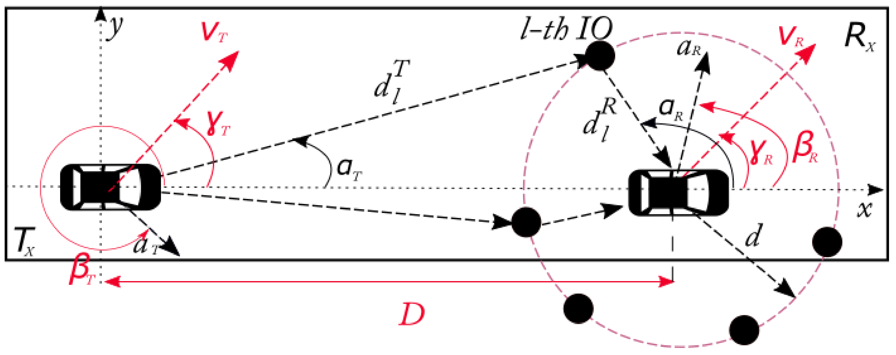
2.2. Single Ring Geometrical Scattering Channel Model

To test the channel estimation techniques, we need to define how to represent the communication channel. This representation needs to take most critical physical effects of the vehicular environment into consideration, and it also needs to be as close to reality as possible in order to properly evaluate the system performance.
Considering that the vehicular channel does not fulfill the WSSUS condition, the channel representation proposed in [14,15,16] is used in this work. The channel introduced in [14,15,16] is a statistical geometrical model for mobile-to-mobile systems. The scenario has a mobile transmitter with variable velocity and acceleration, as well as a receptor moving at a variable velocity and acceleration. The receiver is surrounded by interfering objects positioned in a circle whose center is the receptor itself. Therefore, the model depicts a realistic representation of a mobile to mobile system scenario. Furthermore, the model proposed in [14,15,16] is physically complete but mathematically simple in comparison with other non-WSSUS geometry-based statistical channel models.
In the model presented in Figure 5, V T corresponds to the vector describing the velocity of the transmitter, V R is the vector describing the velocity of the receptor, a T represents the vector describing the acceleration of the transmitter, a R denotes the vector describing the acceleration of the receptor, d comes to be the radius of the ring, and l- t h > I O corresponds to the l- t h interfering object. As a result, the channel transfer function is given as follows [14,15,16],
h ( τ , t ) = l = 1 L g l e x p { j [ θ l 2 π f c τ l ( t ) ] } δ [ t τ l ( t ) ] Ω T 0 ( t t 0 ) ,
where f c corresponds to the central frequency of the OFDM signal, whereas g l , θ l , and α l P are random variables. Specifically, g l is a complex attenuation factor and follows a uniform distribution between [ 0 , 1 2 L ] , θ l is the phase shift that follows a uniform distribution between [ 0 , 2 π ] , and α l p is the angle between the l- t h > I O and the transmitter or receiver and follows a uniform distribution between [ 0 , 2 π ] . However, Ω T 0 ( t t 0 ) is a windowing function equal to 1 if t [ t 0 , t 0 + T 0 ] and 0 otherwise, where t 0 is the reference point where the observation begins and T 0 is the length of the observation window. This windowing function is used in order to ignore the large scale effects. The time-varying propagation delays of the multipath components are given as [14,15,16],
τ l ( t ) = d l T + d l R c t f c f l S + f ˙ l S ( t ) 2 ,
where f l S and f ˙ l S are the Doppler frequency shift caused by the vehicles’ velocity and acceleration, respectively, and are defined in the following form,
f l S = f m a x T c o s ( α l T γ T ) + f m a x R c o s ( α l R γ R ) ,
f ˙ l S ( t ) = f ˙ m a x T ( t ) c o s ( α l T β T ) + f ˙ m a x R ( t ) c o s ( α l R β R ) ,
where d l T , d l R are the distances of the transmitter and the receiver to the l t h I O , c is the speed of light, whereas γ T and γ R are the velocity vector angles of the transmitter and receiver velocity vector, respectively. At the same time, β T and β R are the acceleration vector angles of the transmitter and receiver, respectively. Finally, f m a x P = V P / λ c and f ˙ m a x P ( t ) = a P ( t ) / λ c characterize the maximum Doppler shift caused by the velocity and acceleration of the mobiles, respectively, where λ c stands for the wavelength of the transmitted signal and P must be replaced by R or T, which describes the receptor or the transmitter, respectively [6,17].

2.3. Extreme Learning Machine

The ELM is a learning algorithm for feed-forward artificial neural networks characterized by a single hidden layer [18,19]. The ELM tends to minimize the training error thanks to the adoption of the smallest norm of the output weights. In addition, the ELM has a fast learning speed, as the only parameters that need to be optimized are the output weights between the hidden neurons and the output layer. The computational time required for training can be considered negligible in comparison with traditional feed-forward neural networks and support vector machines [20].
Generally, for a given training set with N m instances { U , T } = { u i , t i } i = 1 N m , where u i = [ u i 1 , u i 2 , . . . , u i D i ] R D i is an input sample and t i = [ t i 1 , t i 2 , . . . , t i D o ] R D o is its corresponding output (the input dimension D i and output dimension D o are not necessarily equal), the output of an standard single hidden layer feed forward network can be written in the following form [18,19],
t ^ k = i = 1 n h β i E L M G [ w i · u ( k ) + b i ] , k = { 1 , N m } ,
where n h is the number of hidden neurons, β i E L M R 1 x D 0 is the weight vector connecting the i-th neuron in the hidden layer with the output neurons, G is the activation function, w i R N m x 1 is the weight vector describing connections of the i-th hidden neuron with the input neurons, and b i is the i-th hidden neuron’s threshold. In the ELM algorithm, input weights w i and bias b i are randomly generated according to a probability distribution and are related by the inner product operator (·).
The training process of the ANN can be expressed as a linear regression problem for the ELM algorithm, where a zero training error between the target output and the actual output ( i = 1 N m t k t k ^ ) can be determined as follows [18,19]
T = F β E L M ,
where the output matrix of the hidden layer acquires the form of
F = G ( w 1 · u 1 + b 1 ) . . . G ( w n h · u 1 + b n h ) . . . . G ( w i · u j + b i ) . . . . G ( w 1 · u N m + b 1 ) . . . G ( w n h · u N m + b n h ) .
The optimal solution to the ELM can be computed as
β E L M * = F T ,
where F is the Moore-Penrose generalized inverse of F. If we consider zero training error, over-fitting could appear into the ELM algorithm. In order to avoid this problem, calculations are done by minimizing the final weights β E L M with the inclusion or a regularization parameter. In other words, the mean square error is given by
min β E L M , e 1 2 | | β E L M | | 2 + C 2 i = 1 N m | | e i | | 2 ,
s . t f ( u i ) β E L M = t i T e i T , i = 1 , . . . , N m ,
where f ( u ) represents an o u t p u t ( r o w ) vector of matrix in expression (8), e i R D o is the error vector with respect to the i- t h input sample, and C corresponds to the penalty coefficient, must be any real positive number. Finally, its solution when F has more rows than columns ( n h > N m ), can be written as follows [18,19]
β E L M * = F T F + I n h C 1 F T T ,
where I n h is an identity matrix with dimension n h . On the other hand, in the case that F has less rows than columns ( n h < N M ), the previous solution can be written as follows
β E L M * = F T F F T + I N m C 1 T ,
where I N m is an identity matrix with dimension N m . In summary, the training algorithm of the ELM is given in Algorithm 1.
Algorithm 1: ELM algorithm.
Electronics 10 00968 i001

2.4. Semi-Supervised Extreme Learning Machine

In a semi supervised setting, we have few labeled data and plenty of unlabeled data, which can be used to increase the perform of the system [18]. For this approach, we assume that the distribution of the label data is similar to the distribution of the unlabeled data and try to extract that the beneficial information. The SS-ELM algorithm is presented in Algorithm 2.
Algorithm 2: SS-ELM algorithm.
Electronics 10 00968 i002
It is important to notice that λ is known as the trade-off parameter, and indicates how important the unlabeled data are in the training stage. Obviously, if we set this parameter to zero, then the SS-ELM matches the standard ELM. The Laplacian graph is used to extract the geometry distribution information contained in the available data. As previously indicated, one of the assumptions of SS learning is that both labeled data U l and unlabeled data U μ are drawn from the same marginal distribution P U . Another assumption is that the conditional probabilities of P ( t | u 1 ) and P ( t | u 2 ) should be similar if the two points u 1 and u 2 are close. With these assumptions, the manifold regularization term is usually minimized with the following function [20]
L m = 1 2 i , j r i , j | | P ( t | u i ) P ( t | u j ) | | 2 ,
where r i , j is the pair-wise similarity between two inputs and can be computed with the next expression
r i , j = exp ( | | u i u j | | 2 / 2 σ 2 ) if u i , u j are neighbors 0 otherwise ,
Expression (13) can be simplified as L m = T r ( T ^ T L T ^ ) , where T r ( · ) is the trace of a matrix. The Laplacian graph can be calculated as L = D R , where D is a diagonal matrix with its diagonal elements D i i = j = 1 l + μ r i , j , and the similarity matrix R = [ r i , j ] . As mentioned, the SS-ELM setting incorporates the manifold regularization to incorporate the use of unlabeled data, thus improving the accuracy of the predictions. The expressions for β E L M shown on Algorithm 2 are obtained when modifying the problem on Equation (10) as follows,
min β 1 2 | | β E L M | | 2 + 1 2 i = 1 N m C i | | e i | | 2 + λ 2 T r ( β E L M T F T L F β E L M ) ,
s . t f ( u i ) β E L M = t i T e i T , i = 1 , . . . , N m .
In the context of V2V communications, this algorithm might offer a better performance, as it could, for example, learn from the time and frequency variations present in the propagation scenario. Even though it may learn from these variations, other algorithms that use these dependencies have a large performance degradation [6,8] in the presence of rougher propagation scenarios, like the STA algorithm.

3. Proposed SS-ELM Equalizer

Initially, we used the original ELM with supervised learning (as a reference case). To this end, we performed the training step by employing the two long training symbols as input training data and by following the steps of the Algorithm 1, then the frame was equalized by feeding each data subcarrier to the ELM. As any equalizer, this procedure is done frame by frame. Based on the poor BER resulting from this type of ELM (as will be depicted in the next Section), for this manuscript, we explored the SS learning paradigm for the ELM algorithm along with localized mapping. In the following paragraphs, we will define and explain the proposed SS-ELM algorithm.
The proposed SS-ELM algorithm is based on Algorithm 2 and, as a common machine learning approach, has two stages: training and testing. The first one consists of the training phase, in which we use the pilots and the two long training symbols to calculate the internal parameters of the ELM ( β E L M ). Notice that the weights and biases between the input and hidden layers are arbitrarily generated (a main characteristic of the ELM algorithm as mentioned in Section 2.3) based on the uniform distribution on [−1,1] [21,22]. Using these parameters, we then perform the evaluation phase. Here, we equalize the constellation symbols and, afterwards, calculate the BER metric by using the standard demodulation.
The time-frequency fluctuations in the channel can be seen in Equations (2) and (3) where τ ( t ) represents the general time delay variations. Instead, the several parameters on Equations (4) and (5) show the frequency oscillations associated with the Doppler effect. Consequently, if we feed all the data directly to the model, we will not properly address this problem (as observed in the next Section). Consequently, we perform the training and equalization by considering the frequency and time domains for the SS-ELM algorithm.
The basic ELM architecture consists of two real inputs R { Y i ( k ) } and I { Y i ( k ) } , one for the real part of the constellation symbol and other for its imaginary part, n h hidden neurons, and two neurons on the output, one for each part of the constellation symbol. For the sake of simplicity, we will refer to the inputs as Y i ( k ) and the outputs as Y i ^ ( k ) . First of all, by considering that the channel changes rapidly in the frequency domain, the information from the pilot carriers is used in a localized manner, as shown in Figure 6.
Therefore, four localized equalization processes following the IEEE 802.11p standard are done at the same time, i.e., one for each pilot subcarrier. We define the slot signal as follows
X i p ( k ) , Y i p ( k ) = X i ( k ) , Y i ( k ) k = p p + q ,
where i is the number of OFDM symbol, k denotes the subcarrier number, p represents the pilot corresponding to the slot being process, and q comes to be the length of the frequency slot.
With the localized mapping, there are 12 data carriers for each pilot. This number of data carriers was adopted because it corresponds to the relationship N S D / N S P , where N S D and N S P are given by the parameters exposed in Table 1. Consequently, we take advantage of the frequency dependency of the channel in order to diminish the impact of the frequency variations in the channel in the system performance, since the term λ in Equations (4) and (5) is the closest to the pilot subcarrier term. Then, for each slot, the process is performed symbol by symbol in the time domain by considering the definition given in Equation (1). This is done in order to track the time fluctuations in the channel. For illustration purposes, Figure 6 also represents how the subcarriers are distributed for each slot.
In addition, the block diagram of the equalization process is presented in Figure 7 for clarification purposes. Obviously, it begins when the FFT module is performed and ends with the constellation symbols to be demapped. As can be seen, a pre-equalization with the LS method is done right after the Fourier-based block. The reason behind this stage is because the channel estimation which resulted from the LS scheme for the time domain OFDM symbols is fairly accurate, and results in a good initial mitigation of the channel effects with relatively low computational impact [13].
In addition, an extra design parameter ( δ ) is introduced to strengthen the learning phase in the time domain. This determines how many pilots in the time domain are used for each training step of each slot. This parameter is important as it uses the time dependency of the channel to improve the estimation/equalization processes by considering that the vehicular environment changes rapidly over the time domain. According to our observations, and as is expected in this scenario, a high value of δ might have a negative impact on the system performance. Evidently, the proposed scheme (Figure 7) replaces the channel estimation and equalization blocks seen in Figure 2, by combining them into a single operation after the FFT module. To depict the general operation of the novel SS-ELM equalizer step by step, the SS-ELM training and testing is presented in Algorithm 3.
It is important to consider that the actual value of unlabeled data used for the training of each data frame is the multiplication of μ with the number OFDM symbols N s y m b o l s and the number of slots. Even though the values that are shown in the next Section are small, these values do not directly represent the total amount of data used for the unsupervised learning step of the SS-ELM scheme. Finally, each slot can be processed parallel to each other, by allowing the reduction in the execution time needed to process a full data frame. In fact, this procedure is done in Section 4.4 to estimate the complexity of the proposal.
Algorithm 3: SS-ELM training and equalization.
Electronics 10 00968 i003

4. Simulation Results and Discussions

To further validate our proposal (SS-ELM), we evaluated other state-of-the-art schemes; these techniques are LS, STA, CDP, and C-ELM [13]. For the case of the LS, STA, and CDP schemes, Zero Forcing (ZF) is used as the channel equalize [23]. For comparison results, note that among the several ML-based approaches reported in the literature, we included the C-ELM method, as it has shown the best BER performances without computational cost, not only for communications through optical fiber [21,22] but also for advanced wireless communication systems [13,24,25,26,27]. Of course, these works are not focused on IEEE 802.11p-based V2V communication systems, which present a harsh non-stationary, time-varying, frequency-selective channel; refer to Section 2. On the other hand, it is worth noting that our proposal works with strictly real data (a single constellation symbol is divided into its quadrature and in-phase parts) and consists of a semi-supervised machine learning (a combination of supervised and unsupervised learning). While the C-ELM [13] represents fully complex neural networks under only supervised learning. Furthermore, the C-ELM neural network needs a bounded and differentiable activation function defined in the complex plane and cannot follow semi-supervised training, which limits its generalization ability. Each one of these models is tested in two different system setups. Further details regarding the system setups are given in the subsequent lines. A Monte Carlo simulation of 21 iterations is used to ensure statistical regularity. A total of 10.000 data frames are transmitted in each iteration, and E b / N 0 ranging between 0 to 20 dB that correspond to real-life scenarios [28] are used in the evaluations. The parameters used to perform the simulations are shown in Table 1 and Table 2. Specifically, Table 1 illustrates the IEEE 802.11p system parameters for a 10 MHz channel, whereas Table 2 shows the evaluated system configurations.
Both system configurations simulate an urban environment, with speeds lower than 50 km/h. The first configuration depicts a scenario in which the transmitter is accelerating and changing lanes in preparation to overtake the receiver [29], whereas the second configuration is a scenario in which the receiver is taking an intersection while the transmitter remains in the same lane. For clarification purposes, the parameters that originate the overtake and intersection scenarios (the movement angles, acceleration angles, and velocities of the transmitter and receiver, and initial distance) are shown in bold in Table 2. In this sense, these parameters are highlighted with a red color in Figure 5, where they can also be easily distinguished. Furthermore, the simulations are done with Binary Phase Shift Keying (BPSK). This is because, with BPSK, we have the slowest data rates, as well as the most robust transmissions, which are critical in safety applications. To conclude this part, in order to find the sub-optimal hyper-parameters of the SS-ELM and compare the performance of the different models, we will present the results as a function of the BER and E b / N 0 .

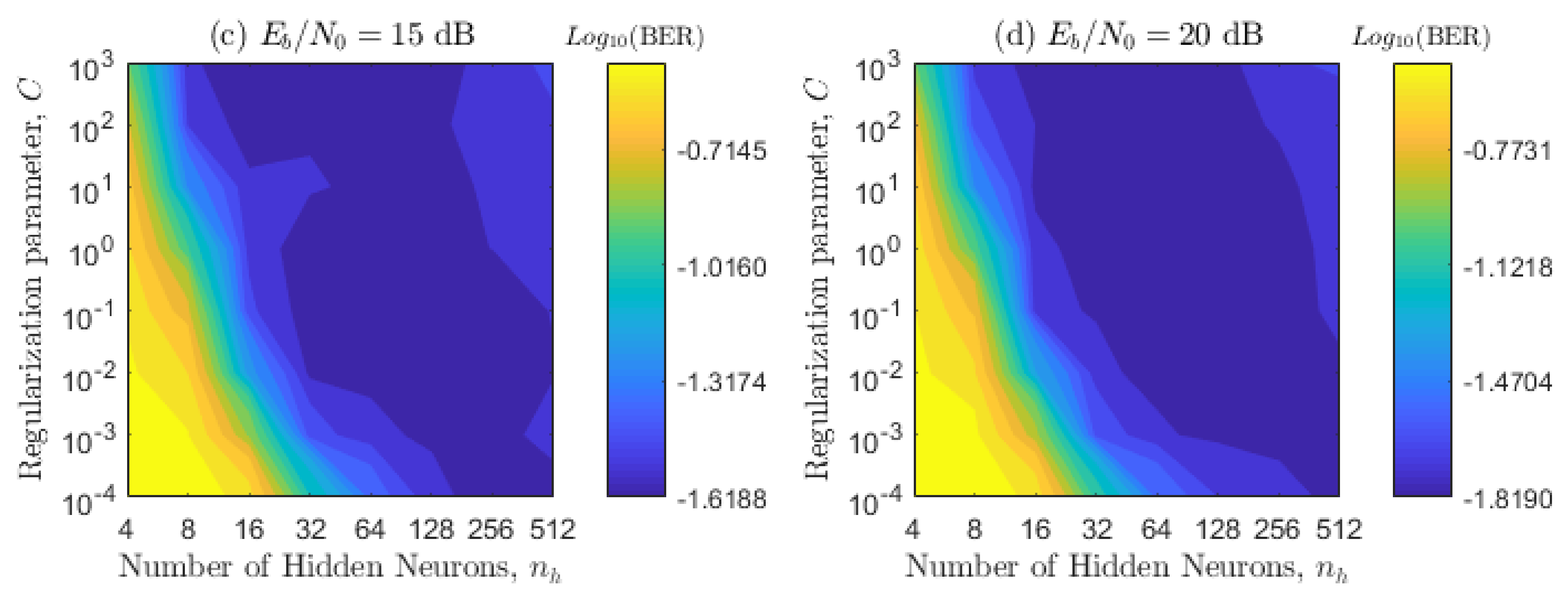
4.1. Numerical Optimization of the SS-ELM Hyper-Parameters
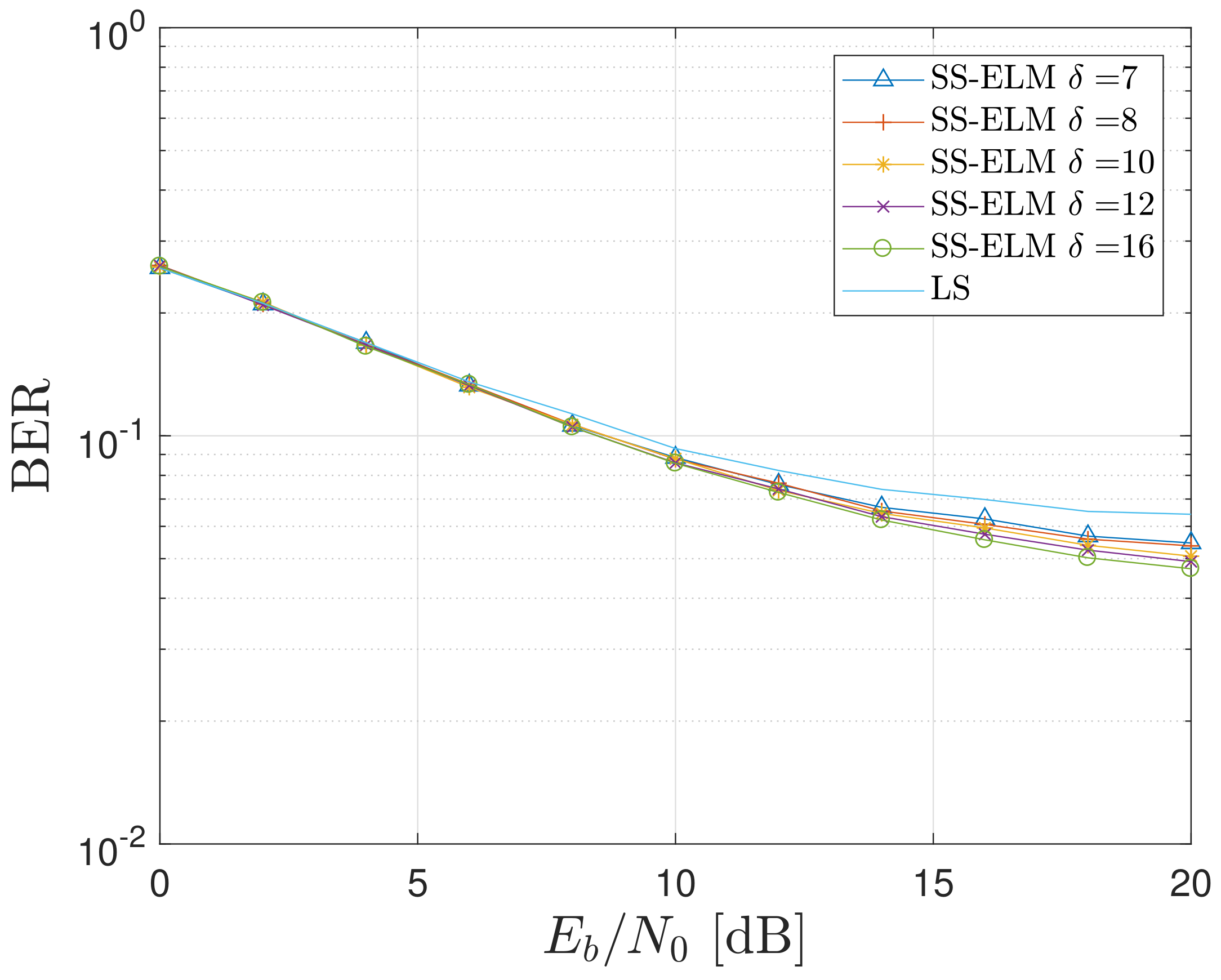
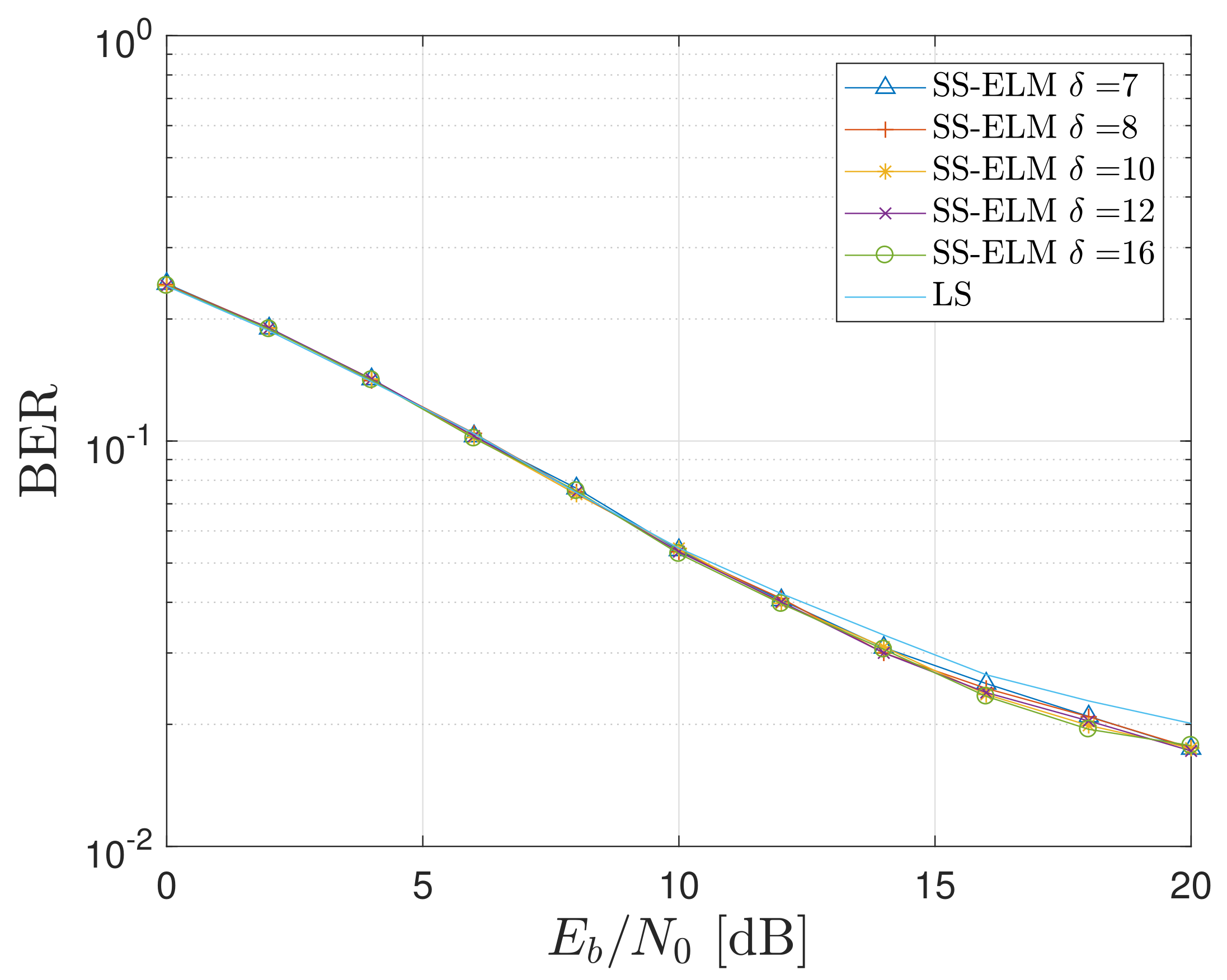
The proposed scheme has several parameters that need to be optimized, and some of these parameters have a correlation between them, so they need to be optimized together. Throughout the paper, we adopt the sigmoid mapping function, since it has reported an excellent generalization ability [18,22]. We initially optimized the regularization parameter C and the number of hidden neurons n h , by considering λ = 0 and μ = 0 . This means that the first optimization is basically the same for a supervised ELM. To select the best parameters, we use contour plots, which are obtained for four E b / N 0 values: 5, 10, 15, and 20 dB for the two channel configurations presented in Table 2. In Figure 8 and Figure 9, each point of the contour plot corresponds to the representative BER value obtained by following the Monte Carlo simulation explained at the beginning of this Section. Then, to select the sub-optimal values of the regularization parameter and number of hidden neurons that minimize the system performance, we use visual inspection. Namely, the areas with the best performance (blue zones) and overlap among most of the figures are chosen. All sub-figures in Figure 8 and Figure 9 are considered in order to obtain a BER invariant to the movement angles, acceleration angles, and velocities of the transmitter and receiver. As expected, these plots also verify that the BER decreases as the relationship E b / N 0 increases.
In Figure 8 and Figure 9, we can see that there is a trade-off between the optimized parameters and the ELM predictability. When the number of hidden neurons is increased, it is possible to decrease the value of the regularization parameter C without compromising the BER performance. In general, the system performance severally decreases if the number of hidden neurons does not exceed the value of 24, specially for regularization parameters lower than 10 0 . Furthermore, if both simulation configurations are compared, it can be observed that the BER metric decreases from configuration 1 to 2 and that the area of the optimal parameters increases from configuration 1 to 2. Based on the previous observations, we selected C = 10 1 and n h = 64 , namely, a pair of hyper-parameters that are inside the optimal area of both configurations. This adoption also considers that the ELM architecture is kept simple, namely, a minimum number of hidden neurons is selected. It is important to notice that the apparent optimal area increases from configuration 2 to 1, which indicates that, for bigger velocity values, the optimal area may be bigger and will probably contain the ones shown above.
Once the values of C and n h were optimized, we proceed to optimize the parameters λ and μ simultaneously for the SS-ELM training/testing, in the same way as the previous ones for the standard ELM. Remember that λ represents the trade-off parameter between the supervised and no-supervised learning and μ proportionally represents the number of unlabeled samples; refer to the end of Section 3. Note that, for these results, we use a linear representation of the BER instead of a logarithmic one because the results are closer to each other and the resulting areas are smaller. Looking at the results of Figure 10 and Figure 11, it can bee seen that the optimal areas are relatively smaller when compared with the ones shown in Figure 8 and Figure 9. This means that there is a smaller range of values that can be used without compromising the BER performance. Furthermore, the values obtained are more sensitive to different channel configurations. It can also be seen in Figure 10 and Figure 11 that, when the value of the parameter μ is higher than 7, the system performs poorly. This result indicates that the proposed SS-ELM algorithm suffers over-fitting, or that there is too much noise added to the training process with the unlabeled data inclusion. When considering the parameter λ , it can be seen that the better values tend to be bigger than 10 0 for the first configuration, and bigger than 10 1 for the second configuration. This behavior means that SS-ELM benefits from bigger values of λ , meaning that the non-labeled data have a big impact on a one-to-one comparison with the labeled data. Then, the selected parameters are λ = 100 and μ = 6 , because this combination shows the best overall results for the simulated configurations. Finally, considering that the total value of unlabeled data used to train each data frame is μ = 6 times N s y m b o l s = 128 times 4, the total value used is 3072 symbols; when we compare this number with the total number of labeled data available for the training (616 symbols), we can observe that we use approximately five times more unlabeled data than labeled data for the training procedure. Hence, we take advantage of the semi-supervised paradigm, where we have few labeled data and plenty of unlabeled data. Transforming this to the studied communication scenario, we have only four pilot subcarriers to equalize 52 data subcarriers, but we use unlabeled data to improve the performance.

4.2. Impact of the δ Parameter on the BER Metric

In this Subsection, we analyze the results of the proposed SS-ELM for different values of the δ parameter. As mentioned in Section 3, the δ parameter is oriented to decrease the time-variant channel effects in the system performance. To this end, it relates to the number of pilot subcarriers employed in the learning phase of each time slot.
In Figure 12 and Figure 13, it can be seen the BER resulted from the SS-ELM scheme against E b / N 0 for diverse δ parameters by considering configurations 1 and 2, respectively. The LS results are also displayed as a reference BER curve. In the following Section, our proposal will be carefully compared with the bench-marking estimators/equalizers. There is a direct relation between the value of the parameter δ and the BE performance. We can also see that, for system configuration 1, there is a clear improvement, with values of δ near to 12; this enhancement is not present for configuration 2. Therefore, it is possible to say that the impact of the parameter δ in the performance of the systems is higher for a rougher system setting, such as the configuration 2. Finally, there is a clear performance improvement for the close interval between 7 and 12 of the parameter δ for both of the evaluated configurations. In conclusion, the best overall results are obtained with a SS-ELM characterized by δ = 16 , by relaxing the E b / N 0 requirement with respect to the LS technique.

4.3. Performance Comparison

In this Subsection, we compare the results between the LS, STA, CDP, traditional ELM, C-ELM [13] techniques, and our proposal, which is based on a SS-ELM neural network. For the standard ELM, the regularization parameter and the number of hidden neurons are the same as the SS-ELM, namely C = 10 and n h = 64 . Furthermore, in our proposal, the rest of the hyper-parameters are the following: λ = 100 , μ = 6 , and 16. Remember that these adoptions are done in order to minimize the system performance (see Section 4.2). According to [13], we adopt 512 hidden neurons and the arcsinh mapping function for the C-ELM.
For the first and second configuration, Figure 14 and Figure 15 depict the BER as a function of E b / N 0 for the different techniques evaluated. It can be seen that ELM, C-ELM, SS-ELM, and LS methods tend to have the same BER, regardless of the scenario. On the other hand, for the first and second configurations, the STA method has the worst and best BER values, respectively. The CDP method outperforms the other techniques for high SNRs only for the first configuration. These observations mean that STA and CDP do not perform uniformly for different channel configurations; consequently, these techniques are not feasible for V2V communications. Among the rest of the evaluated techniques, our proposal shows a uniform and slightly better performance for the evaluated scenarios, especially for higher SNRs. For instance, given a threshold of B E R = 10 1 in the first configuration, the SS-ELM allows a E b / N 0 greater than 8 dB. Meanwhile, the E b / N 0 requirement corresponds to 9, 10, and 14 dB in the case where the LS, ELM, and C-ELM approaches are used, respectively. It is worth noting that observations for SNRs greater than 20 dB can be discarded, since these values rarely occur in real settings [28]. Furthermore, it is worth noting that the vehicular communication channel evaluated in this manuscript is extremely harsh; therefore, none of the evaluated schemes achieved the BER threshold given by the standard and equal to 10 3 [30,31].
The superiority reported in our proposal can be explained by the use of the ELM neural network along with the exploitation of the semi-supervised machine learning scheme. With respect to conventional neural network learning algorithms, the ELM algorithm has demonstrated a better generalization performance in the presence of linear and no-linear distortions [13]. Its generalization ability comes from the parameter neurons between adjacent layers are found by reaching both the smallest training error and the smallest norm of output weights. On the other hand, semi-supervised learning has been applied to several classification and regression tasks with excellent results, in which both the labeled and unlabeled data are used to improve accuracy over supervised approaches. It occurs especially when insufficient training information is available [20]. The reason behind this is that unlabeled data naturally provide valuable information for exploring the data structure in the input space. To conclude this explanation, it is well known that the interactions among different types of impairments (such as the harsh time-varying, frequency-selective channel considered in this manuscript) are not effectively considered and handled for non-based ML-based schemes [6]. For instance, STA and CDP techniques were not designed considering the characteristics of the vehicular channel. In regular channels, STA uses frequency dependencies to improve the performance, but in vehicular communications, the channel varies rapidly in frequency, explaining the poor results for rougher channels. Meanwhile, CDP suffers greatly from low E b / N 0 because it uses the channel estimation iteratively to equalize the channel, so, in high noise environments, this estimation is contaminated, decreasing the performance.

4.4. Execution Time Analysis

In this Subsection, we evaluate the performance of the addressed techniques in terms of execution time, which is the time required by the algorithms to complete the processing (from the FFT module to the parallel to serial converter, see Figure 2). As the execution time is hardware/software dependent, Table 3 is presented to show the hardware configuration used in the simulations. Regarding software features, Matlab R2017a has been used to perform the evaluation. To measure the representative interval times, we follow the Monte Carlo simulation explained at the beginning of Section 4 by fixing the channel model parameters at arbitrary values, since these do not interfere in the estimation of the processing times. Because each of the frequency slots shown in Figure 6 has a localized submapping estimation and equalization, the slots can be processed independently from each other, thus decreasing the execution time of the proposed SS-ELM scheme by a factor of 4 due to the number of pilots in an OFDM symbol (refer to Figure 6). The results of this experiment are depicted in Table 4 under the name of parallel SS-ELM.
The results of Table 4 depict that the proposed SS-ELM increases the execution time by around 19 times compared to the CDP estimator for instance, and when optimized with parallel computing, the execution time is reduced to 167 ± 2.6 ms, increasing the time to approximately nine times. Note that although the SS-ELM scheme requires the largest operation time among the evaluated techniques, its execution time is still far from the upper limit of latency equal to 300 ms [5] specified by ETSI for safety applications. It is important to consider that these results are software/hardware-dependent, so the results may vary from device to device. Finally, considering that the computer processing units that modern cars have on board are powerful, the overall results of the proposed algorithm are sufficient to justify an increase in the execution time. This is especially important for safety applications in vehicular communications, where a low BER is vital to ensure the reliability of the information. Considering the execution time. the proposed algorithm is suitable for safety applications such as collision risk warning or road hazard signaling [5]. However, its use for critical safety applications such as pre-crash sensing should be investigated further.
Note that although the proposed SS-ELM scheme has the longest execution time with respect to the compared models, we conclude that it is possible to further reduce the learning and/or operation time of the scheme by having only one layer forward, e.g., on an Field-Programmable Gate Array (FPGA) [32]. In future work, we will explore the use of FPGAs to implement the proposed scheme, analyse the impact of a larger sample size of δ , the possibility of applying unsupervised configurations as an alternative to semi-supervised ones, and analyse the impact of using channel coding schemes in different system configurations.

5. Conclusions

This work demonstrates the feasibility of using ML algorithms as an alternative to classical techniques, used in wireless communication systems, to estimate and equalize the vehicular communication channel. A channel estimation and equalization algorithm based on extreme learning machines was designed and tested over two different channel system configurations: overtake and intersection scenarios.
An improved version of an SS-ELM channel estimator and equalizer was introduced for vehicular communications considering the 802.11p amendment. The proposed SS-ELM scheme outperformed the extreme learning machine (ELM) and the fully complex extreme learning machine (C-ELM) algorithms for the evaluated scenarios. Furthermore, the proposed SS-ELM scheme performed similarly compared to other traditional techniques. The proposed scheme had a better performance for lower E b / N 0 values compared to STA and CDP for the first and second system configurations, respectively, considering that E b / N 0 values in wireless environments are usually lower than 20 dB.
We analyzed the impact that δ has on the equalization process, and concluded that there is still room for improvement when considering rougher channel configurations than the ones shown in this work. As the value of δ increases, the algorithm requires a longer execution time, but a larger δ enhances the performance of the algorithm, it becomes suitable for optimization.
Finally, the execution time of the proposed model was simulated on a general-purpose computer with an interpreted language such as Matlab, for a fair comparison with the other models. Even though the SS-ELM scheme requires the largest execution time among the evaluated techniques, it still falls within the latency window specified by the standard.

Author Contributions

Conceptualization, E.S., C.A.A.-M. and D.Z.-B.; methodology, E.S. and D.Z.-B.; software, E.S. and D.Z.-B.; formal analysis, E.S.; investigation, E.S.; writing—original draft preparation, D.Z.-B., C.A.A.-M., S.B., E.S. and I.S.; writing—review and editing, D.Z.-B., C.A.A.-M., S.B., E.S. and I.S.; supervision, C.A.A.-M.; project administration, C.A.A.-M.; funding acquisition, C.A.A.-M. All authors have read and agreed to the published version of the manuscript.

Funding

This research was funded by Vicerrectoría de Investigación y Desarrollo (VID) de la Universidad de Chile Proyecto ENL 01/20.

Conflicts of Interest

The authors declare no conflict of interest.

Abbreviations

The following abbreviations are used in this manuscript:
ANNArtificial Neural Network
AWGNAdditive White Gaussian Noise
BERBit Error Rate
BPSKBinary Phase Shift Keying
CDPConstructed Data Pilots
CFRChannel Frequency Response
CPCyclic Prefix
CPUCentral Process Unit
C-ELMComplex Extreme Learning Machine
C-V2XCellular Vehicular to Anything
DCDirect Current
DLDeep Learning
ELMExtreme Learning Machine
ETSIEuropean Telecommunication Standards Institute
FFTFast Fourier Transform
FPGAField-Programmable Gate Array
GPUGraphics Processing Unit
IFFTInverse Fast Fourier Transform
LSLeast Squares
MLMachine Learning
MMSEMinimum Mean-Square Error
OFDMOrthogonal Frequency Division Multiplexing
PHYPhysical Layer
RAMRandom Access Memory
SSSemi-Supervised
SS-ELMSemi Supervised Extreme Learning Machine
STASpectral Temporal Averaging
SNRSignal to Noise Ratio
VCSVehicular Communication Systems
V2VVehicle to Vehicle
V2IVehicle to Infrastructure
WiFiWireless Fidelity
WSSUSWide-Sense Stationary Uncorrelated Scattering
ZFZero Forcing

References

  1. Ahmed, E.; Gharavi, H. Cooperative Vehicular Networking: A Survey. IEEE Trans. Intell. Transp. Syst. 2018, 19, 996–1014. [Google Scholar] [CrossRef] [PubMed]
  2. Wang, J.; Liu, J.; Kato, N. Networking and Communications in Autonomous Driving: A Survey. IEEE Commun. Surv. Tutor. I 2019, 21, 1243–1274. [Google Scholar] [CrossRef]
  3. ETSI TR 102 638 V1.1.1: Intelligent Transport Systems (ITS), Vehicular Communications, Basic Set of Applications, Definitions. Available online: https://www.etsi.org/deliver/etsi_tr/102600_102699/102638/01.01.01_60/tr_102638v010101p.pdf (accessed on 9 January 2015).
  4. ETSI. TS 101 539-2 V1.1.1: Intelligent Transport Systems (ITS), V2X Applications, Part 2: Intersection Collision Risk Warning (ICRW) Application Requirements Specification 1. Available online: https://www.etsi.org/deliver/etsi_ts/101500_101599/10153902/01.01.01_60/ts_10153902v010101p.pdf (accessed on 30 June 2018).
  5. ETSI. TS 101 539-3 V1.1.1: Intelligent Transport Systems (ITS), V2X Applications, Part 3: Longitudinal Collision Risk Warning (LCRW) Application Requirements Specification. Available online: https://www.etsi.org/deliver/etsi_ts/101500_101599/10153903/01.01.01_60/ts_10153903v010101p.pdf (accessed on 30 November 2013).
  6. Ortega, N.M.; Azurdia-Meza, C.A.; Gutierrez, C.A.; Maciel-Barboza, F.M. On the Influence of the non-WSSUS Condition in the Performance of IEEE 802.11-Based Channel Estimators for Vehicular Communications. In Proceedings of the IEEE 10th Latin-American Conference on Communications (LATINCOM), Guadalajara, Mexico, 14–16 November 2018; pp. 1–6. [Google Scholar] [CrossRef]
  7. 802.11-2016 - IEEE Standard for Information technology—Telecommunications and information exchange between systems Local and metropolitan area networks—Specific requirements - Part 11: Wireless LAN Medium Access Control (MAC) and Physical Layer (PHY) Specifications; IEEE Std 802.11-2012 (Revision of IEEE Std 802.11-2007); IEEE: Miami, FL, USA, 2016; pp. 1–3534. [CrossRef]
  8. Zhao, Z.; Cheng, X.; Wen, M.; Jiao, B.; Wang, C. Channel Estimation Schemes for IEEE 802.11p Standard. IEEE Intell. Transp. Syst. 2009, 5, 38–49. [Google Scholar] [CrossRef]
  9. Fernandez, J.; Borries, K.; Cheng, L.; Kumar, B.V.K.V.; Stancil, D.D.; Bai, F. Performance of the 802.11p physical layer in vehicle-to-vehicle environments. IEEE Trans. Veh. Tech. 2018, 61, 3–14. [Google Scholar] [CrossRef]
  10. Ye, H.; Liang, L. Machine Learning for Vehicular Networks. arXiv 2018, arXiv:1712.07143. [Google Scholar]
  11. Ye, H.; Li, G.; Juang, B. Power of Deep Learning for Channel Estimation and Signal Detection in OFDM Systems. IEEE Wirel. Commun. Lett. 2018, 7, 114–117. [Google Scholar] [CrossRef]
  12. Sattiraju, R.; Weinand, A.; Schotten, H. Channel Estimation in C-V2X using Deep Learning. In Proceedings of the 2019 IEEE International Conference on Advanced Networks and Telecommunications Systems (ANTS), Goa, India, 16–19 December 2019. [Google Scholar]
  13. Liu, J.; Mei, K.; Zhang, X.; Ma, D.; Wei, J. Online Extreme Learning Machine-Based Channel Estimation and Equalization for OFDM Systems. IEEE Commun. Lett. 2019, 23, 1276–1279. [Google Scholar] [CrossRef]
  14. Gutiérrez, C.; Pätzold, M.; Dahech, W.; Youssef, N. A Non-WSSUS Mobile-to-Mobile Channel Model Assuming Velocity Variations of the Mobile Stations. In Proceedings of the 2017 IEEE Wireless Communications and Networking Conference (WCNC), San Francisco, CA, USA, 19–22 March 2017. [Google Scholar] [CrossRef] [Green Version]
  15. Gutierrez, C.; Gutierrez-Mena, J.; Luna-Rivera, J.; Campos-Delgado, D.; Velazquez, R.; Patzold, M. Geometry-Based Statistical Modeling of Non-WSSUS Mobile-To-Mobile Rayleigh Fading Channels. IEEE Trans. Veh. Technol. 2018, 1, 362–377. [Google Scholar] [CrossRef] [Green Version]
  16. Jaime-Rodríguez, J.J.; Gómez-Vega, C.A.; Gutiérrez, C.A.; Luna-Rivera, J.M.; Campos-Delgado, D.U.; Velázquez, R. A non-WSSUS channel simulator for V2X communication systems. Electronics 2020, 9, 1190. [Google Scholar] [CrossRef]
  17. Gutiérrez, C.A.; Pätzold, M.; Ortega, N.M.; Azurdia-Meza, C.; Maciel-Barboza, F.M. Doppler shift characterization of wideband mobile radio channels. IEEE Trans. Veh. Technol. 2019, 68, 12375–12380. [Google Scholar] [CrossRef]
  18. Huang, G.; Song, S.; Gupta, J. Semi-supervised and unsupervised extreme learning machines. IEEE Trans. Cybern. 2014, 12, 2405–2417. [Google Scholar] [CrossRef]
  19. Souza, P.V.d.C.; Torres, L.C.B.; Silva, G.R.L.; Braga, A.d.P.; Lughofer, E. An advanced pruning method in the architecture of extreme learning machines using l1-regularization and bootstrapping. Electronics 2020, 9, 811. [Google Scholar] [CrossRef]
  20. Li, S.; Song, S.; Wan, Y. Laplacian twin extreme learning machine for semi-supervised classification. Neurocomputing 2018, 321, 17–27. [Google Scholar] [CrossRef]
  21. Zabala-Blanco, D.; Mora, M.; Azurdia-Meza, C.A.; Dehghan Firoozabadi, A.; Palacios Játiva, P.; Soto, I. Relaxation of the Radio-Frequency Linewidth for Coherent-Optical Orthogonal Frequency-Division Multiplexing Schemes by Employing the Improved Extreme Learning Machine. Symmetry 2018, 8, 632. [Google Scholar] [CrossRef] [Green Version]
  22. Zabala-Blanco, D.; Mora, M.; Azurdia-Meza, C.A. Dehghan Firoozabadi, Extreme Learning Machines to Combat Phase Noise in RoF-OFDM Schemes. Electronics 2019, 12, 921. [Google Scholar] [CrossRef] [Green Version]
  23. Ijiga, O.E.; Ogundile, O.O.; Familua, A.D.; Versfeld, D.J. Review of channel estimation for candidate waveforms of next generation networks. Electronics 2019, 8, 956. [Google Scholar] [CrossRef] [Green Version]
  24. Liu, N.; Wang, H. Ensemble based extreme learning machine. IEEE Signal Process. Lett. 2010, 17, 754–757. [Google Scholar] [CrossRef]
  25. Carrera, D.F.; Zabala-Blanco, D.; Vargas-Rosales, C.; Azurdia-Meza, C.A. Extreme Learning Machine-Based458Receiver for Multi-User Massive MIMO Systems. IEEE Commun. Lett. 2021, 25, 484–488. [Google Scholar] [CrossRef]
  26. Yang, L.; Zhao, Q.; Jing, Y. Channel Equalization and Detection with ELM-Based Regressors for OFDM Systems. IEEE Commun. Lett. 2019, 24, 86–89. [Google Scholar] [CrossRef]
  27. Carrera, D.F.; Vargas-Rosales, C.; Yungaicela-Naula, N.M.; Azpilicueta, L. Comparative Study of Artificial Neural Network Based Channel Equalization Methods for MmWave Communications. IEEE Access 2021, 9, 41678–41687. [Google Scholar] [CrossRef]
  28. Shivaldova, V.; Winkelbauer, A.; Mecklenbrauker, C. Signal-to-noise ratio modeling for vehicle-to-infrastructure communications. In Proceedings of the 2014 IEEE 6th International Symposium on Wireless Vehicular Communications (WiVeC 2014), Vancouver, BC, Canada, 14–15 September 2014. [Google Scholar] [CrossRef]
  29. Ortega, N.M.; Azurdia-Meza, C.A.; Gutierrez, C.A.; Gómez-Vega, C.A. Second Order Statistics and BER Performance Analysis of a non-WSSUS V2X Channel Model that Considers Velocity Variations. In Proceedings of the 2019 IEEE Latin-American Conference on Communications (LATINCOM), Salvador, Brazil, 11–13 November 2019; pp. 1–6. [Google Scholar] [CrossRef]
  30. U.S. Department of Transportation. Vehicle Safety Communications Project V Final Report; Report DOT HS 810 591; National Highway Traffic Safety Administration: Washington, DC, USA, 2006.
  31. Feukeu, E.; Djouani, K.; Kurien, A. An MCS Adaptation Technique for Doppler Effect in IEEE 802.11p Vehicular Networks. Procedia Comput. Sci. 2013, 19, 570–577. [Google Scholar] [CrossRef] [Green Version]
  32. Frances-Villora, J.V.; Rosado-Muñoz, A.; Bataller-Mompean, M.; Barrios-Aviles, J.; Guerrero-Martinez, J.F. Moving learning machine towards fast real-time applications: A high-speed FPGA-based implementation of the OS-ELM training algorithm. Electronics 2018, 7, 308. [Google Scholar] [CrossRef] [Green Version]
Figure 1. Block diagram of the OFDM transmitter.
Electronics 10 00968 g001
Figure 2. Block diagram of the OFDM receiver.
Electronics 10 00968 g002
Figure 3. IEEE 802.11p subcarrier distribution.
Electronics 10 00968 g003
Figure 4. IEEE 802.11p packet preamble structure.
Electronics 10 00968 g004
Figure 5. Single ring geometrical channel scattering model. The vehicle on the left side is the transmitter, while the vehicle on the right side represents the receiver.
Electronics 10 00968 g005
Figure 6. Subcarrier distribution slots.
Electronics 10 00968 g006
Figure 7. Block diagram of the equalization process.
Electronics 10 00968 g007
Figure 8. BER countour plot in terms of the regularization parameter C, number of hidden neurons, and different E b / N 0 values for system configuration 1.
Electronics 10 00968 g008
Figure 9. BER countour plot in terms of the regularization parameter C, number of hidden neurons, and different E b / N 0 values for system configuration 2.
Electronics 10 00968 g009aElectronics 10 00968 g009b
Figure 10. BER contour plot of λ and μ for different E b / N 0 values and system configuration 1.
Electronics 10 00968 g010
Figure 11. BER contour plot of λ and μ for different E b / N 0 values and system configuration 2.
Electronics 10 00968 g011
Figure 12. BER of the proposed SS-ELM scheme with δ as parameter and the LS algorithm for system configuration 1.
Electronics 10 00968 g012
Figure 13. BER of the proposed SS-ELM scheme with δ as parameter and the LS algorithm for system configuration 2.
Electronics 10 00968 g013
Figure 14. BER as a function of E b / N 0 for different evaluated techniques and system configuration 1.
Electronics 10 00968 g014
Figure 15. BER as a function of E b / N 0 for different evaluated techniques and system configuration 2.
Electronics 10 00968 g015
Table 1. IEEE 802.11p system parameters for a 10 MHz channel.
ParameterValue
Number of data subcarriers ( N S D ) 48
Number of pilot subcarriers ( N S P )4
Number of subcarriers total ( N S T )52
Subcarrier frequency spacing ( Δ f )0.15625 MHz
IFFT/FFT periods ( T F F T )6.4 µs (1/ Δ f )
PHY preamble duration ( T P R E A M B L E )32 µs
Duration of the
Signal BPSK-OFDM symbol ( T S I G N A L )
8 µs
Training symbol guard interval duration ( T G I )3.2 µs
Symbol interval ( T s y m )8 µs
Short training sequence duration ( T S H O R T )16 µs
Long training sequence duration ( T L O N G )16 µs
Table 2. Simulation parameters.
ParameterConfiguration 1Configuration 2
Carrier Frequency ( f c )5.9 GHz5.9 GHz
Bandwidth (B)10 MHz10 MHz
ModulationBPSKBPSK
Number of OFDM symbols per package (L)128128
Transmitter velocity ( V T )40 km/h20 km/h
Receiver velocity ( V R )40 km/h20 km/h
Transmitter movement angle ( γ T )105°10°
Receiver movement angle ( γ R )70°70°
Transmitter acceleration angle ( β T )105°15°
Receiver acceleration angle ( β R )250°70°
Initial distance (D)300 m100 m
Radius of the ring (d)30 m30 m
Table 3. Computational system specifications.
ComponentModel
Central Processing Unit (CPU)Intel i5 10400F
2.9 GHz–4.1 GHz
Random Access Memory (RAM)16 GB 2133 MHz
Graphics Processing Unit (GPU)GTX1060 6 GB
Table 4. Algorithm execution times.
AlgorithmTime [ms]
LS0.0269 ± 0.0095
STA13.5 ± 0.344
CDP18.4 ± 0.471
ELM40.5 ± 5.1
C-ELM [13]127 ± 9.74
SS-ELM658 ± 10.4
Parallel SS-ELM167 ± 2.6
Publisher’s Note: MDPI stays neutral with regard to jurisdictional claims in published maps and institutional affiliations.

