
Adaptive Fading Extended Kalman Filtering for Mobile Robot Localization Using a Doppler–Azimuth Radar


1
School of Intelligent Manufacturing, Luoyang Institute of Science and Technology, Luoyang 471023, China
2
Henan International Joint Laboratory of Cutting Tools and Precision Machining, Luoyang Institute of Science and Technology, Luoyang 471023, China
3
Department of Mechanical Engineering, Politecnico di Milano, 20156 Milan, Italy
*
Authors to whom correspondence should be addressed.
Electronics 2021, 10(20), 2544; https://doi.org/10.3390/electronics10202544
Submission received: 11 September 2021
/
Revised: 9 October 2021
/
Accepted: 13 October 2021
/
Published: 18 October 2021
(This article belongs to the Special Issue 10th Anniversary of Electronics: New Advances in Systems and Control Engineering)
Abstract
:In this paper, the localization problem of a mobile robot equipped with a Doppler–azimuth radar (D–AR) is investigated in the environment with multiple landmarks. For the type (2,0) robot kinematic model, the unknown modeling errors are generally aroused by the inaccurate odometer measurement. Meanwhile, the inaccurate odometer measurement can also give rise to a type of unknown bias for the D–AR measurement. For reducing the influence induced by modeling errors on the localization performance and enhancing the practicability of the developed robot localization algorithm, an adaptive fading extended Kalman filter (AFEKF)-based robot localization scheme is proposed. First, the robot kinematic model and the D–AR measurement model are modified by considering the impact caused by the inaccurate odometer measurement. Subsequently, in the frame of adaptive fading extended Kalman filtering, the way to the addressed robot localization problem with unknown biases is sought out and the stability of the developed AFEKF-based localization algorithm is also discussed. Finally, in order to testify the feasibility of the AFEKF-based localization scheme, three different kinds of modeling errors are considered and the comparative simulations are conducted with the conventional EKF. From the comparative simulation results, it can be seen that the average localization error under the developed AFEKF-based localization scheme is and the average localization errors using the conventional EKF are , and , respectively, under the three cases of the constant bias, the white Gaussian stochastic bias and the bounded uncertainty bias.
1. Introduction
Because of the extensive applications of mobile robots in diverse fields, such as aerospace, intelligent industry and intelligent transportation, and so on, many efforts have been made on the studies of the robot. As an essential issue and a research hot topic in the robot field, the localization problem has attracted much research attention [1,2]. For robot localization problems, various types of external sensors, including inertial sensors [3], LIDAR [4,5], Doppler–azimuth radar [6] (D–AR) and ultrasonic sensors [7], have been used to obtain the measurements. Among them, the D–AR with the merits of lower cost, smaller size and lighter weight, has obtained initial attention in the robot localization problem. To the best of authors’ knowledge, only a few study results can be found in the existing literature, see, for example, [6,8,9,10,11]. For instance, in a given environment where the associations between landmarks and the D–AR are known, an extended Kalman filter (EKF) is employed to perform the robot localization in [6], where the D–AR is equipped on the robot platform to output the measurements containing the Doppler frequency shift and the azimuth. In Reference [11], regarding a specific case in which the associations between landmarks and the D–AR are unknown, a particle filtering-based localization scheme has been proposed.
It is worth mentioning that, for the kinematic model of a type (2,0) robot, both of the displacement and angular velocities are obtained by the odometer measurement [4]. The above-mentioned results all acquiesce in that the odometer measurement can be acquired precisely. Notwithstanding, in reality, owing to the aging of electronic components, it is unavoidable that the sensitivity of the odometer would be attenuated, which would result in an inaccurate measurement output of the odometer. In general, such inaccurate measurement is usually treated as a kind of inaccurate measurement-induced unknown bias, which can lead to modeling errors. If such a situation takes place, the kinematic model cannot accurately characterize the robot’s state, comprising the position and the orientation. If not taken into consideration adequately, a satisfactory localization performance cannot be achieved and may even cause the localization error divergence. Therefore, for the considered robot localization problem, it is necessary to take the inaccurate odometer measurement-induced unknown bias into consideration, which motivates the current study.
In the existing literature, one of the commonly used schemes is to introduce model uncertainties accounting for inaccurate measurement-induced unknown bias, see, for example [12,13]. For the sake of decreasing the effect of model uncertainties on the system performance, a number of approaches have been developed and, accordingly, some representative research results have been published for linear systems [14], nonlinear systems [15], master–slave systems [16], neutral systems [17], robotic manipulators [18], unmanned aerial vehicles [19] and marine vehicles [20]. It is noted that, among them, certain induced positive scalars have been presented in the process of dealing with uncertainties. By suitably adjusting these induced scalars, the desired system performance can be met. This feature means that the solution to deal with uncertainties is not suitable for on-line use. Owing to the fact that the robot system has a high realtime requirement and strong mobility, it is unrealistic to dynamically adjust the induced scalars to cut down the effect of uncertainties and to satisfy the realtime system performance.
For making up for the above-mentioned drawbacks, in the presence of unknown modeling errors, an adaptive fading KF (AFKF) for linear Gaussian systems has been proposed by introducing a forgetting factor, which can be adjusted adaptively, to suppress the influence of the uncertainties and a stronger tracking performance has also been achieved by comparison with the conventional KF in [21,22]. For nonlinear Gaussian systems, the corresponding AFEKF algorithm has been developed under the conventional EKF frame and some early research interests have been reported [23,24,25]. Moreover, a few practical engineering problems have been solved by utilizing such an adaptive algorithm [26,27]. For example, in Reference [26], a multiple fading factors-based adaptive KF algorithm has been proposed for the unmanned underwater vehicle navigation. In Reference [27], the speed and the load torque estimation problem has been investigated for induction motors by using the AFEKF. Until now, the localization problem of applying the AFEKF algorithm to constrain the impact of unknown modeling errors is still open, and this composes the principal focus of our present study.
Inspired by the above discussions, this paper aims to investigate the localization problem of the robot with unknown modeling errors by using the AFEKF algorithm. The main challenges we will encounter are identified as follows:
- How to characterize the inaccurate odometer measurement-induced unknown bias in the kinematic model of a type (2,0) robot?
- How to consider the inaccurate odometer measurement-induced unknown bias in the D–AR measurement model?
- How to developed a on-line localization algorithm such that the given localization performance can be achieved?
In this paper, we strive to meet the above-mentioned challenges and the main contributions are as follows:
- The inaccurate odometer measurement-induced unknown bias is considered in the kinematic model of a type (2,0) robot for the first time;
- The induced unknown bias is regarded in the D–AR measurement model;
- The AFEKF is adopted to reduce the impact of the modeling errors and achieving on-line localization;
- Thee comparative simulations have been conducted to testify the usefulness of the developed AFEKF by choosing three different types of modeling errors.
The remainder of this paper is arranged as follows. Section 2 states the considered robot localization problem. Section 3 shows the conventional EKF algorithm. In Section 4, the AFEKF-based localization algorithm is developed. Section 5 presents the stability analysis of the corresponding algorithm. The practicality of the provided AFEKF-based robot localization method is validated in Section 6 and some conclusions are drawn in Section 7.
2. Problem Formulation
In order to successfully carry out the subsequent analysis, the following assumptions are made.
Assumption A1.
The mobile robots considered in this paper are without the wheel skidding and slipping in modeling and simulation.
Assumption A2.
At each time instant, the Doppler–azimuth radar can collect all the measurements from the associated landmarks.
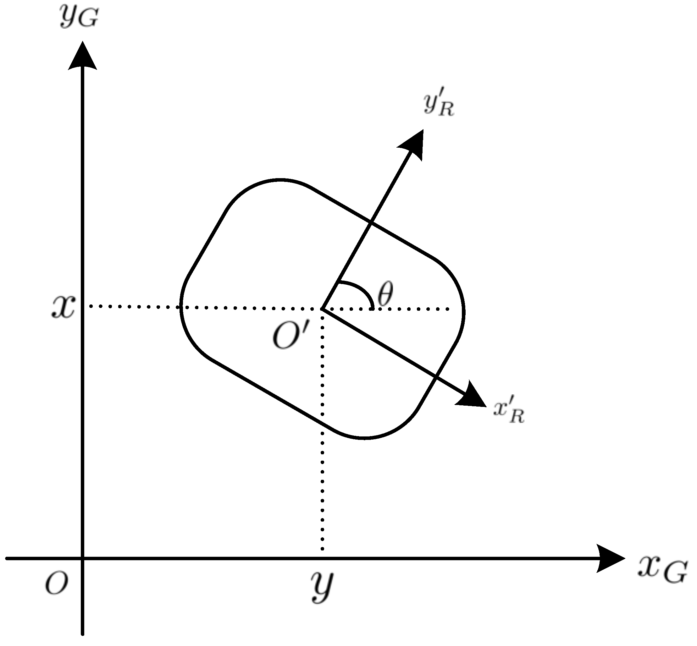
2.1. Conventional Robot Kinematic Model
In this paper, we consider a type (2,0) mobile robot, shown in Figure 1, whose kinematic model is described as follows [28]:
where is the position of the robot, denotes its orientation angle. The displacement velocity v and the angular velocity can be acquired via the odometer measurement. Then, by discretizing the continuous-time system (1), the following discrete-time system can be obtained:
where denotes the sampling interval between two successive time instants, k and .
Denote robot’s state as and treat as the input vector of the robot. Then, taking the system noise into consideration, system (2) can be transformed as:
where , . Here, we assume that the system noise is a white Gaussian stochastic sequence with covariance .
By using the Taylor series to expand the nonlinear function around the estimate , (3) can be expanded as:
where , denotes the higher order terms occurring in the expansion process.
2.2. Doppler-Azimuth Radar Measurement Model
We choose S known coordinates as the positions of the landmarks. Each landmark can produce the Doppler frequency shift. The D–AR installed on the robot platform can collect its measurements. At time instant k, the produced Doppler frequency shift from the lth landmark and the azimuth angle are regarded as a set of measurements. In light of the definitions of the azimuth angle and the Doppler frequency shift in [6], the measurement model associated with the landmark l can be obtained as follows:
where , is the radar carrier frequency and c is the speed of light. Suppose that the measurement noise is a white Gaussian stochastic sequence with covariance .
Taking the total S landmarks into account, the following overall measurement equation can be obtained:
where , , and the augmented measurement noise is with zero mean and covariance where denotes a block-diagonal matrix.
By applying the Taylor series expansion again to expanding the nonlinear measurement model (6), one has:
where
denotes the higher order terms.
Remark 1.
From the robot system model (3) and the Doppler–azimuth radar’s measurement model (6), it can be discovered that the odometer measurements, and , are not only the input state in (3) but are also the parameters involved in the measurement (6). Once the inaccurate odometer measurement-induced unknown modeling errors occur, both the system model and the measurement (6) would be affected. If the system and the measurement models, without considering the impact of the inaccurate odometer measurement-induced unknown bias, are directly used for localization, the localization performance will be attenuated.
This paper aims to develop a feasible scheme to locate the attitude of the robot in the presence of the unknown modeling errors and meanwhile guarantee the localization error exponentially bounded in mean square.
3. The Conventional EKF Algorithm
Under the frame of the conventional EKF, the robot kinematic model needs to be known exactly, and the higher order terms and in (4) and (7), respectively, are neglected. Consequently, the robot system and measurement models can be expressed as:
Then, the following conventional EKF algorithm can be given:
Prediction:
The one-step state prediction:
the one-step predicted error covariance can be derived as:
Then, by putting the one-step predicted state into the measurement model (9), the following measurement prediction can be obtained:
Update:
At sampling time instant , the estimated robot’s state can be obtained via the following constructed filter:
where is the filter gain matrix, which can be derived according to:
The localization error covariance can be denoted as:
Remark 2.
In the conventional EKF algorithm, the filtering performance highly depends on the system and the measurement models, which need to be known completely in advance. However, in practice, some unexpected factors may bring about modeling errors, such as the aging of electronic components, and so on. Moreover, [21] has indicated that the system model inaccuracy may deteriorate the filtering performance and even bring about the divergence of the filtering error. For the sake of working out this problem, the AFEKF method has been proposed to reduce the impact of incomplete modeling information and can maintain the system performance, which is suitable for the robot localization addressed in this paper.
4. Adaptive Fading EKF Algorithm
In this section, for making up the drawbacks of the conventional EKF algorithm, we employ the following AFEKF to cope with the system model’s inaccuracy induced by the inaccurate odometer measurement.
Prediction:
The one-step state prediction:
obtain the innovation
the one-step predicted error covariance is
where is referred to as forgetting factor,
and
Measurement Update:
The filter gain matrix can be computed according to:
the estimated robot’s state can be obtained at sampling time instant via the following filter:
The localization error covariance can be updated by
Remark 3.
According to the AFEKF algorithm (16)–(23), the prominent difference between the conventional EKF and the AFEKF lies in a forgetting factor being inserted into the Equation (18). Such an AFEKF algorithm has the following three features. First, the AFEKF has a unified filter frame and is effective for the filtering problem for nonlinear stochastic systems subject to inaccurate dynamics or measurement. Secondly, the acquisition of the forgetting factor needs a light computational complexity. Thirdly, this adaptive algorithm is suitable for applying to the realtime localization. In the next section, the stability will be analyzed.
5. Stability Analysis
In practical engineering, owing to the aging of electronic components, the odometer cannot always produce the exact measurements used for kinematic modeling. For characterizing such a case and for the convenience of analysis, we introduce an unknown vector to express the odometer measurements deviation. Then, the robot kinematic model (2) can be transformed as:
where , , .
For the convenience of the stability analysis of the developed AFEKF-based localization method, one-step formulation is considered in terms of an a priori variable. Therefore, by employing the Taylor series to expand the nonlinear function around the estimate , it has from (24) that:
where ; expresses the higher order terms in the nonlinear function .
In the addressed robot localization problem, by taking the odometer measurement-induced unknown bias into account, the measurement model (6) can be written as:
where
The measurement model (6) can be expanded as follows:
where
, denotes the higher order terms induced by the expansion of the nonlinear function .
Definition 1.
An AFEKF filter is given as follows:
In terms of Definition 1, letting the localization error be , then, one has:
where , and .
Definition 2.
From the expressions of and , two scalars and can easily be found, such that and . Moreover, we assume , and .
In (25) and (26), the uncertain terms and induced by the odometer measurements are assumed to be bounded and fulfilled,
where and are two positive scalars.
We assume the high order terms and fulfilling:
where , , and are four positive scalars.
Theorem 1.
Given the robot system (25), measurement (27) and the AFEKF algorithm shown in Definition 1, the localization error (29) is exponentially bounded in mean square and bounded with probability one under the following initial condition:
and
where , , , , , , .
Remark 4.
Until now, the localization problem of the robot with modeling errors has been solved by developing the AFEKF algorithm. Moreover, the stability has been discussed. In the next section, by considering three different types of modeling errors, three sets of comparison simulations are implemented to validate the effectiveness of the developed AFEKF-based localization scheme.
6. Simulation Results
In this section, compared with the conventional EKF, three sets of simulations are conducted to testify to the usefulness of the AFEKF-based localization scheme under three different types of modeling errors.
Set the sampling interval as s, and here we regard the sampling interval of the odometer and that of the Doppler Radar as the same. The displacement velocity is chosen as m/s and the angular velocity is set as rad/s, respectively. The system noise covariance is chosen as . Seven landmarks (i.e., ) are deployed in the simulation and the positions of the landmarks are , , , , , , and , respectively. The carrier frequency of the Doppler-a-zimuth radar is set as and the speed of light is set as . The measurement noises covariance is set as . The initial state is a Gaussian stochastic variable with expectation and covariance . The initial positive definite matrix is set as .
Based on the above parameter settings, under the following three different cases, the comparisons between the AFEKF-based algorithm and the conventional EKF method are made by implementing 500 simulation experiments.
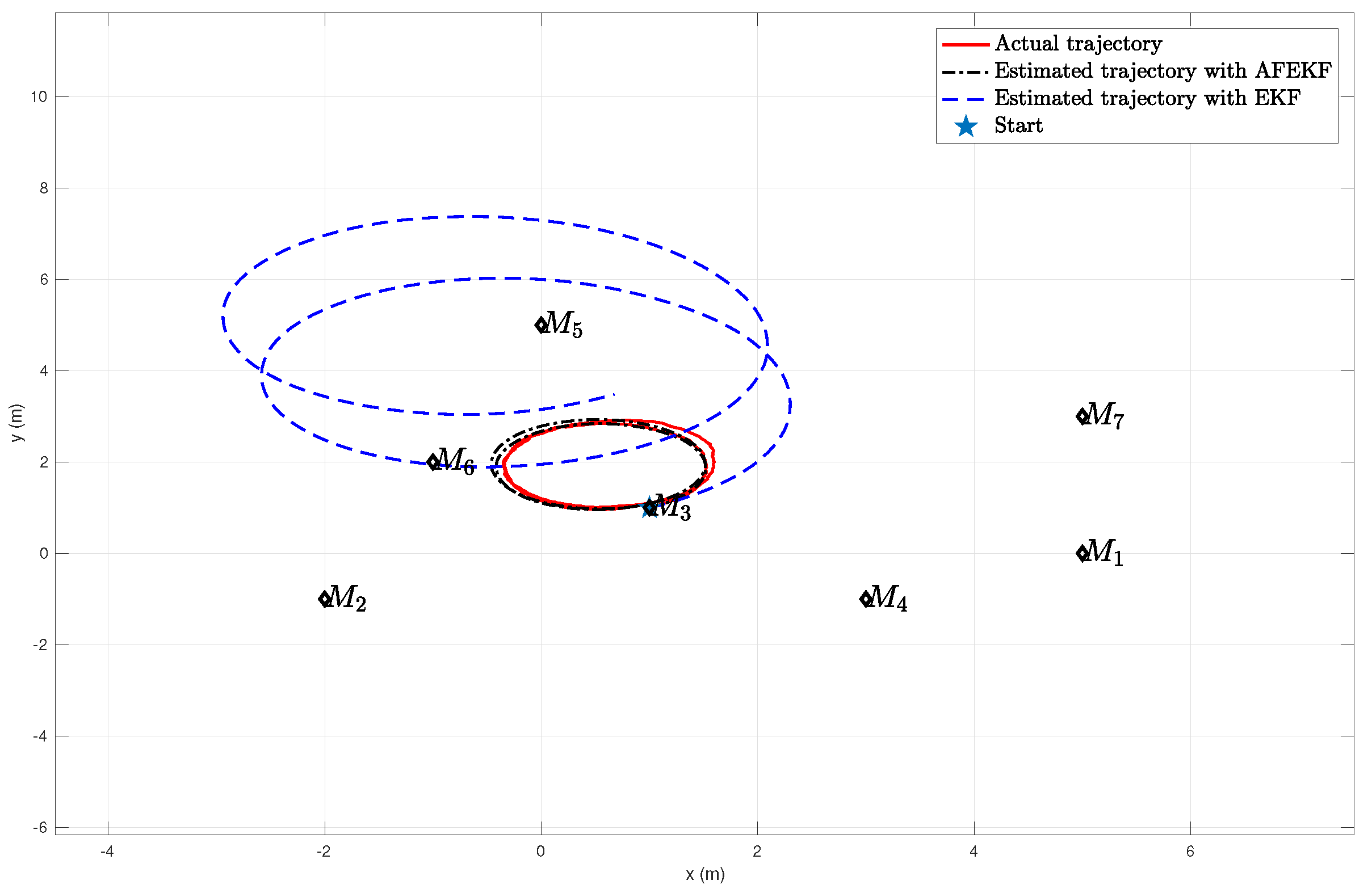
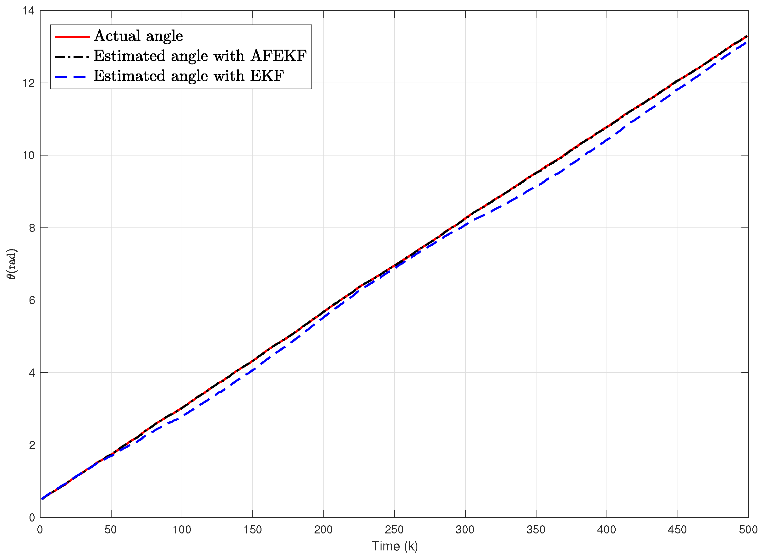
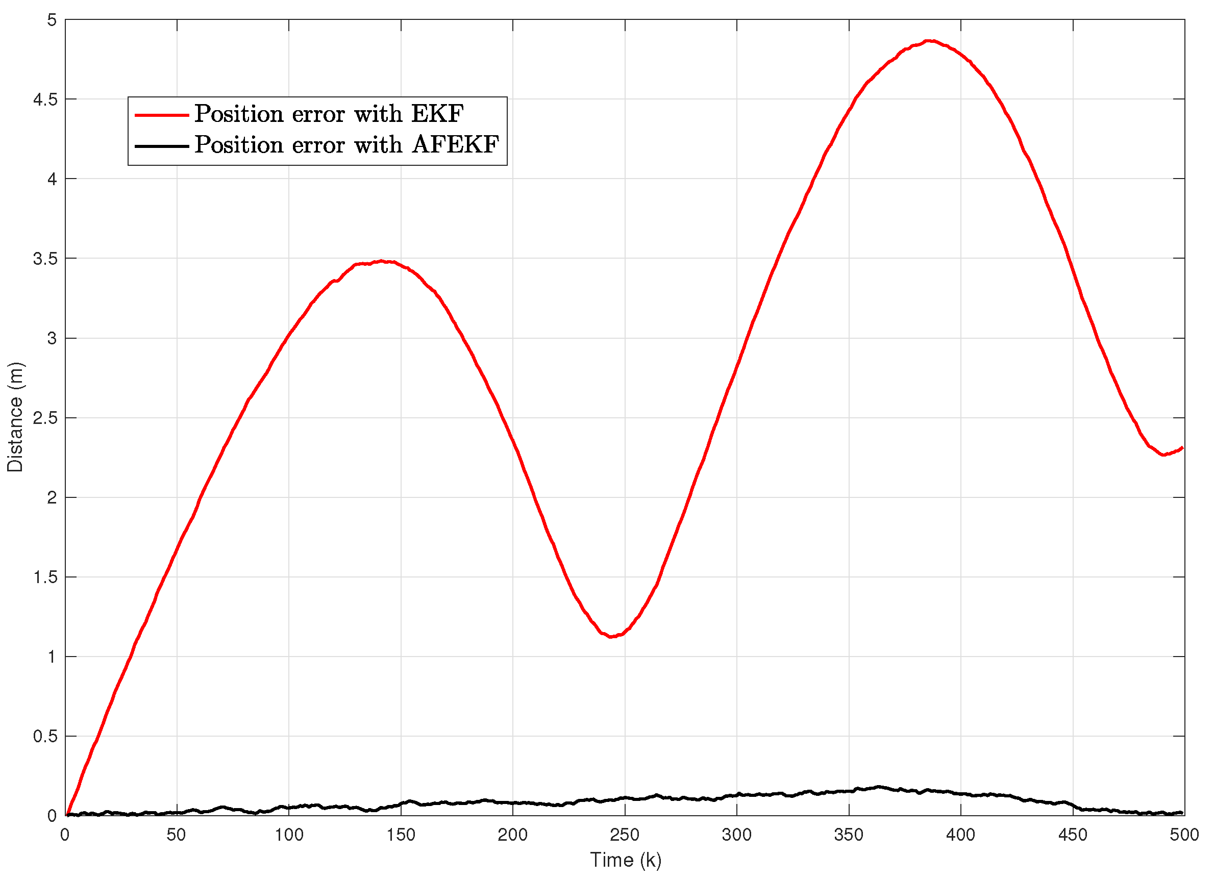
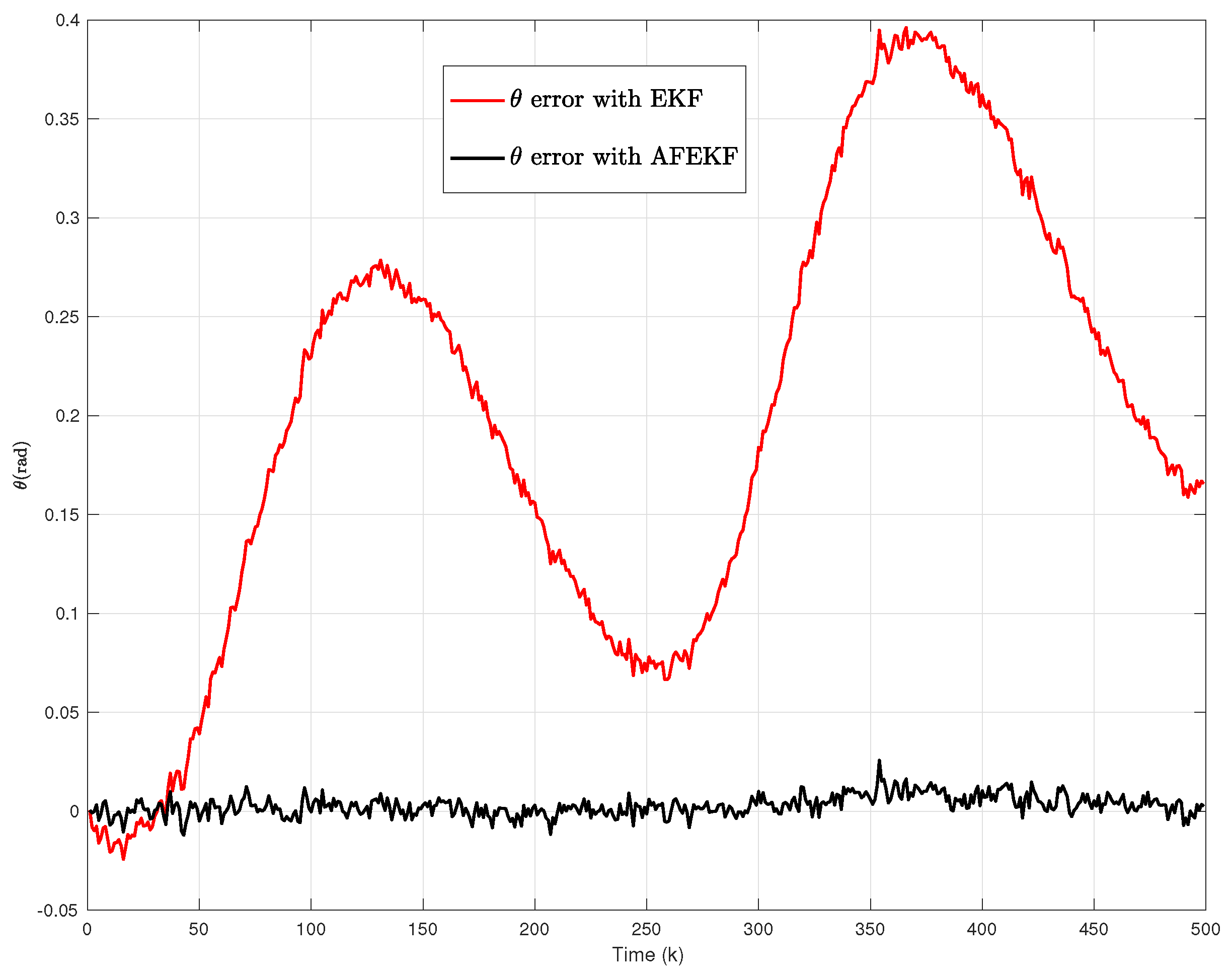
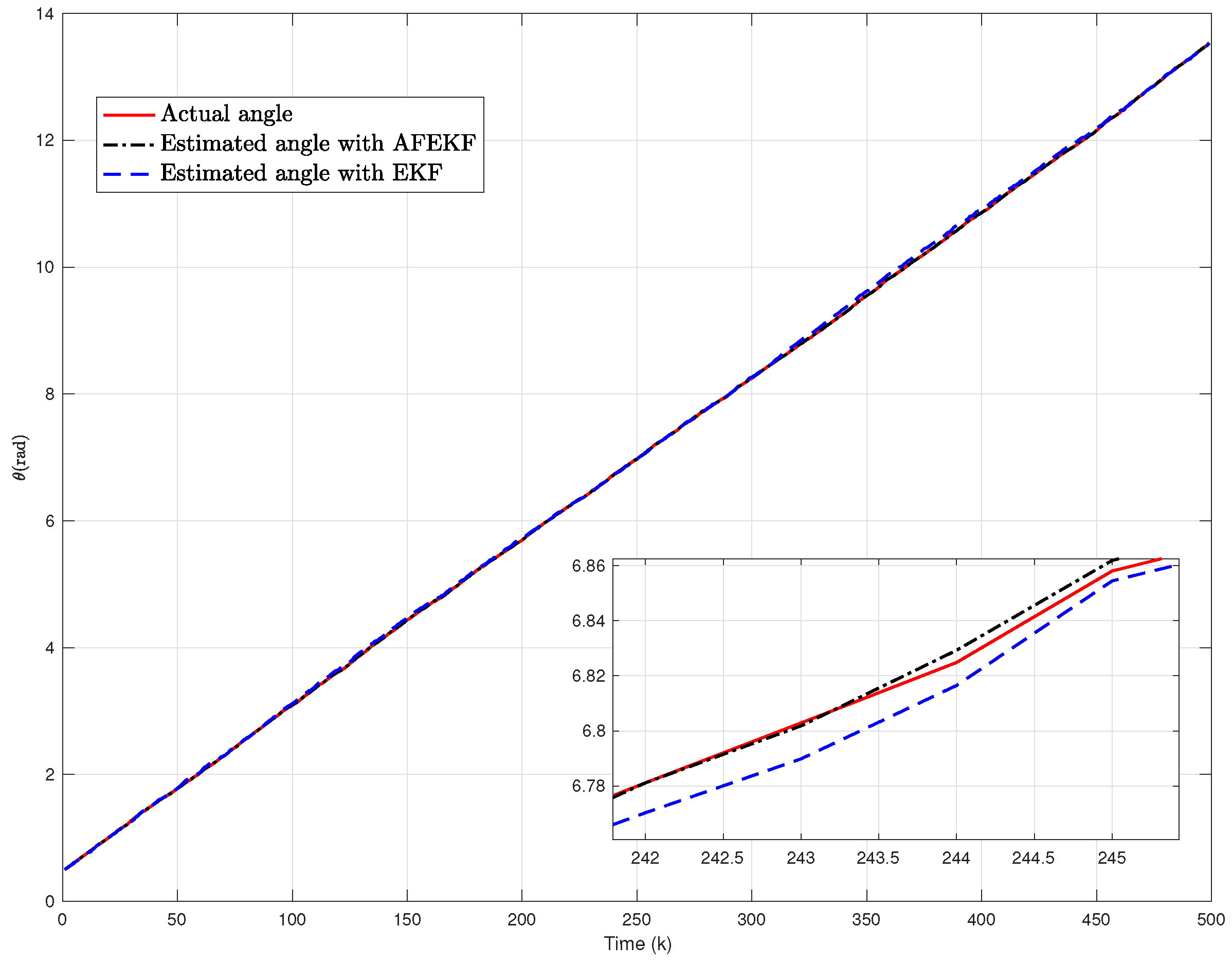
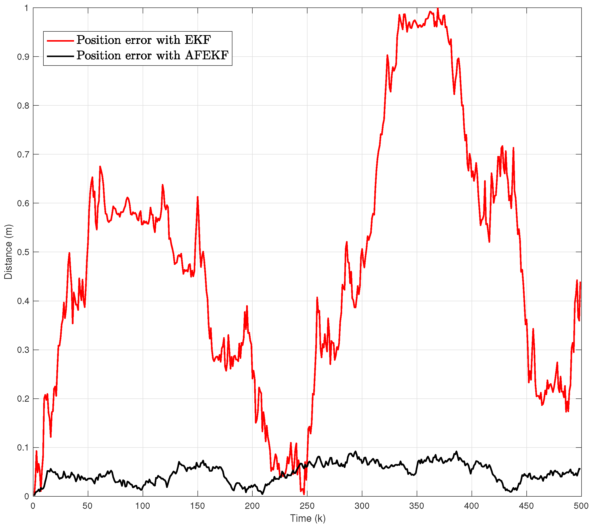
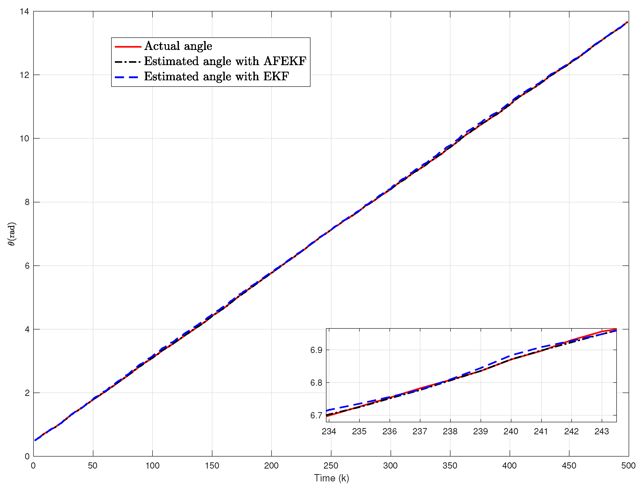
For the first situation, the bias vector is chosen as a constant bias, that is, . In terms of the conventional EKF and the AFEKF algorithms, the simulation outcomes are depicted in Figure 2, Figure 3, Figure 4 and Figure 5, where Figure 2 displays the actual and estimated robot trajectories, Figure 3 depicts the actual and the estimated angles, and Figure 4 and Figure 5 depict the position and the angle errors, respectively.
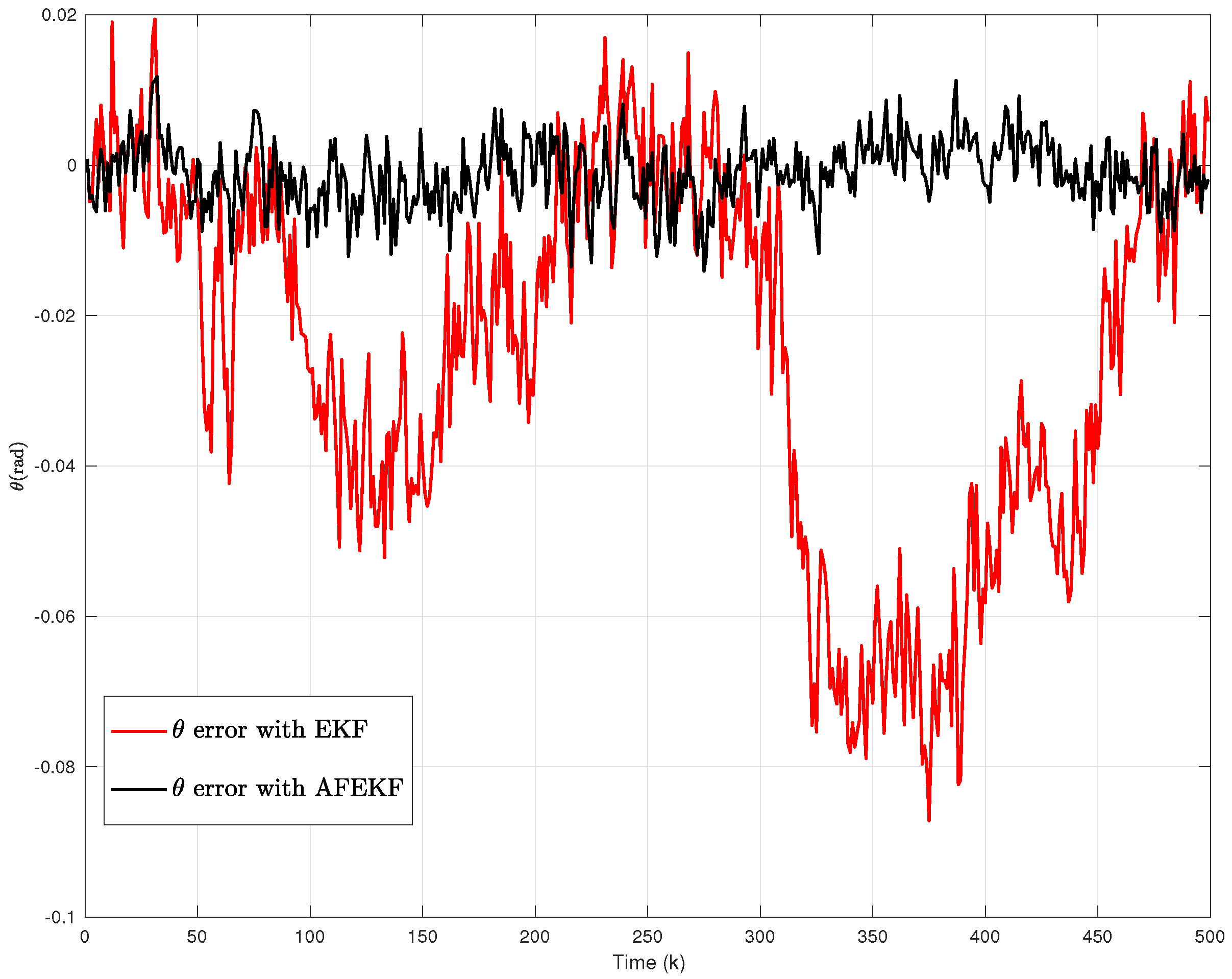
For the second situation, we regard the bias vector as a set of white Gaussian stochastic vectors with variance . The simulation results are listed in Figure 6, Figure 7, Figure 8 and Figure 9, where Figure 6 presents the actual and the estimated robot trajectories, the actual and the estimated angles are shown in Figure 7, and the position and the angle errors are depicted in Figure 8 and Figure 9, respectively.
For the third situation, the bias vector is set as an uncertainty satisfying . The simulation results are given in Figure 10, Figure 11, Figure 12 and Figure 13. The actual and the estimated trajectories are shown in Figure 10. Figure 11 depicts the actual angle and the estimated angle, and Figure 12 and Figure 13 depict the position and the angle errors, respectively.
From the simulation results, it can be seen that the developed AFEKF-based robot localization scheme presents a good localization performance. Specifically, the influence of the modeling errors on the localization performance can be resisted owing to the introduction of the forgetting factor. Moreover, the simulations show that the conventional EKF algorithm has an unsatisfied localization performance, which implies the conventional EKF has poor robustness against the modeling errors.
7. Conclusions
In this paper, in the featured environment with the known association between the sensor and the landmarks, we have studied the localization problem of a mobile robot by developing an AFEKF-based localization scheme. A type of odometer measurement-induced modeling error has been considered for this AFEKF-based robot localization problem. To mitigate the influence of the induced modeling errors and to enhance the robot localization, an AFEKF-based localization scheme has been developed. Three sets of comparative simulations have been conducted to testify to the feasibility of the developed AFEKF-based localization scheme under three sets of different biases, respectively.
Author Contributions
Conceptualization, B.L. and Y.L.; methodology, B.L.; software, B.L.; validation, B.L., Y.L. and H.R.K.; formal analysis, B.L.; investigation, B.L.; resources, B.L.; data curation, B.L.; writing—original draft preparation, B.L.; writing—review and editing, B.L., Y.L. and H.R.K.; visualization, Y.L. and H.R.K.; supervision, Y.L. and H.R.K.; project administration, B.L. and H.R.K.; funding acquisition, B.L. and H.R.K. All authors have read and agreed to the published version of the manuscript.
Funding
This research was funded in part by the Italian Ministry of Education, University and Research through the Project “Department of Excellence LIS4.0-Lightweight and Smart Structures for Industry 4.0”, the National Natural Science Foundation of China grant number 51475222, the Science and Technology Key Project of Henan Province of China grant number 202102210074, the Science Foundation of Henan International Joint Laboratory of Composite Cutting Tools and Precision Machining, and Science Foundation of Luoyang Key Laboratory of Advanced Manufacturing and Cutting Tools.
Conflicts of Interest
The authors declare no conflict of interest.
References
- Chen, S.; Chen, C. Probabilistic fuzzy system for uncertain localization and map building of mobile robots. IEEE Trans. Instrum. Meas. 2012, 61, 1546–1560. [Google Scholar] [CrossRef]
- Fankhauser, P.; Bloesch, M.; Hutter, M. Probabilistic terrain mapping for mobile robots with uncertain localization. IEEE Robot. Autom. Lett. 2018, 3, 3019–3026. [Google Scholar] [CrossRef] [Green Version]
- Lee, S.; Kim, B.; Kim, H.; Ha, R.; Cha, H. Inertial sensor-based indoor pedestrian localization with minimum 802.15.4a configuration. IEEE Trans. Ind. Inform. 2011, 7, 455–466. [Google Scholar] [CrossRef]
- Yang, F.; Wang, Z.; Lauria, S.; Liu, X. Mobile robot localization using robust extended H∞ filtering. Proc. Inst. Mech. Eng. Part I-J. Syst. Control Eng. 2009, 223, 1067–1080. [Google Scholar] [CrossRef] [Green Version]
- Lu, Y.; Shen, B. Mobile robot localization under stochastic communication protocol. Kybernetika 2020, 56, 152–169. [Google Scholar]
- Guan, R.P.; Ristic, B.; Wang, L.; Moran, B.; Evans, R. Feature-based robot navigation using a Doppler-azimuth radar. Int. J. Control 2017, 90, 888–900. [Google Scholar] [CrossRef]
- Khyam, M.O.; Rahim, M.N.A.; Li, X.; Jayasuriya, A.; Mahmud, M.A.; Oo, A.M.T.; Ge, S.S.G. Simultaneous excitation systems for ultrasonic indoor positioning. IEEE Sens. J. 2020, 20, 13716–13725. [Google Scholar] [CrossRef]
- Battistelli, G.; Chisci, L.; Fantacci, C.; Farina, A.; Graziano, A. A new approach for Doppler-only target tracking. In Proceedings of the 16th International Conference on Information Fusion, Istanbul, Turkey, 9–12 July 2013; pp. 1616–1623. [Google Scholar]
- Shames, I.; Bishop, A.N.; Smith, M.; Anderson, B.D.O. Doppler shift target localization. IEEE Trans. Aerosp. Electron. Syst. 2013, 49, 266–276. [Google Scholar] [CrossRef] [Green Version]
- Yang, L.; Yang, L.; Ho, K.C. Moving target localization in multistatic sonar by differential delays and Doppler shifts. IEEE Signal Process. Lett. 2016, 23, 1160–1164. [Google Scholar] [CrossRef]
- Guan, R.P.; Ristic, B.; Wang, L.; Evans, R. Monte Carlo localisation of a mobile robot using a Doppler-azimuth radar. Automatica 2018, 97, 161–166. [Google Scholar] [CrossRef]
- Yang, F.; Wang, Z.; Hung, Y.S. Robust Kalman filtering for discrete time-varying uncertain systems with multiplicative noises. IEEE Trans. Autom. Control 2002, 47, 1179–1183. [Google Scholar] [CrossRef] [Green Version]
- Lu, Y.; Karimi, H.R. Variance-constrained resilient H∞ filtering for mobile robot localization under dynamic event-triggered communication mechanism. Asian J. Control 2021, 23, 2064–2078. [Google Scholar] [CrossRef]
- Xie, L. Output feedback H∞ control of systems with parameter uncertainty. Int. J. Control 1996, 63, 741–750. [Google Scholar] [CrossRef]
- Liu, S.; Wang, Z.; Chen, Y.; Wei, G. Protocol-based unscented Kalman filtering in the presence of stochastic uncertainties. IEEE Trans. Autom. Control 2020, 65, 1303–1309. [Google Scholar] [CrossRef]
- Karimi, H.R. A sliding mode approach to H∞ synchronization of master-slave time-delay systems with Markovian jumping parameters and nonlinear uncertainties. J. Frankl. Inst.-Eng. Appl. Math. 2012, 349, 1480–1496. [Google Scholar] [CrossRef] [Green Version]
- Han, Q.-L. On robust stability of neutral systems with time-varying discrete delay and norm-bounded uncertainty. Automatica 2004, 40, 1087–1092. [Google Scholar] [CrossRef]
- Xiao, B.; Yin, S. Exponential tracking control of robotic manipulators with uncertain dynamics and kinematics. IEEE Trans. Ind. Inform. 2019, 15, 689–698. [Google Scholar] [CrossRef]
- Mu, C.; Zhang, Y. Learning-based robust tracking control of quadrotor with time-varying and coupling uncertainties. IEEE Trans. Neural. Netw. Learn. Syst. 2020, 31, 259–273. [Google Scholar] [CrossRef]
- Karimi, H.R.; Lu, Y. Guidance and control methodologies for marine vehicles: A survey. Control Eng. Pract. 2021, 111, 104785. [Google Scholar] [CrossRef]
- Xia, Q.; Ming, R.; Ying, Y.; Shen, X. Adaptive fading Kalman filter with an application. Automatica 1994, 30, 1333–1338. [Google Scholar] [CrossRef]
- Geng, J. Adaptive estimation of multiple fading factors in Kalman filter for navigation applications. GPS Solut. 2008, 12, 273–279. [Google Scholar] [CrossRef]
- Kim, K.H.; Jee, G.I.; Park, C.G.; Lee, J.G. The stability analysis of the adaptive fading extended Kalman filter. Int. J. Control Autom. Syst. 2009, 7, 49–56. [Google Scholar] [CrossRef]
- Bicer, C.; Babacan, E.K.; Ozbek, L. Stability of the adaptive fading extended Kalman filter with the matrix forgetting factor. Turk. J. Electr. Eng. Comput. Sci. 2012, 20, 819–833. [Google Scholar]
- Haghighi, M.S.; Pishkenari, H.N. Real-time topography and Hamaker constant estimation in atomic force microscopy based on adaptive fading extended Kalman filter. Int. J. Control Autom. Syst. 2021, 19, 2455–2467. [Google Scholar] [CrossRef]
- Wang, J.; Chen, X.; Yang, P. Adaptive H∞ Kalman filter based on multiple fading factors and its application in unmanned underwater vehicle. ISA Trans. 2021, 108, 295–304. [Google Scholar] [CrossRef] [PubMed]
- Zerdali, E.; Yildiz, R.; Inan, R.; Demir, R.; Barut, M. Improved speed and load torque estimations with adaptive fading extended Kalman filter. Int. Trans. Electr. Energy Syst. 2021, 31, e12684. [Google Scholar] [CrossRef]
- Campion, G.; Bastin, G.; Dandrea-Novel, B. Structural properties and classification of kinematic and dynamic models of wheeled mobile robots. IEEE Trans. Robot. Autom. 1996, 12, 47–62. [Google Scholar] [CrossRef]
- Reif, K.; Gunther, S.; Yaz, E.; Unbehauen, R. Stochastic stability of the discrete-time extended Kalman filter. IEEE Trans. Autom. Control 1999, 44, 714–728. [Google Scholar] [CrossRef]
- Lu, Y.; Shen, B.; Shen, Y. Recursive filtering for mobile robot localization under an energy harvesting sensor. Asian J. Control 2021. [Google Scholar] [CrossRef]
- Lu, Y.; Karimi, H.R. Recursive fusion estimation for mobile robot localization under multiple energy harvesting sensors. IET Contr. Theory Appl. 2021. [Google Scholar] [CrossRef]
Figure 1.
Robot model.

Figure 2.
Robot’s trajectory and its estimates under constant bias.

Figure 3.
Robot’s angle and its estimates under constant bias.

Figure 4.
Robot’s position errors under constant bias.

Figure 5.
Robot’s angle errors under constant bias.

Figure 6.
Robot’s trajectory and its estimates under stochastic bias.

Figure 7.
Robot’s angle and its estimates under stochastic bias.

Figure 8.
Robot’s position errors under stochastic bias.

Figure 9.
Robot’s angle errors under stochastic bias.

Figure 10.
Robot’s trajectory and its estimates under uncertainty.

Figure 11.
Robot’s angle and its estimates under uncertainty.

Figure 12.
Robot’s position errors under uncertainty.

Figure 13.
Robot’s angle errors under uncertainty.

Publisher’s Note: MDPI stays neutral with regard to jurisdictional claims in published maps and institutional affiliations. |
© 2021 by the authors. Licensee MDPI, Basel, Switzerland. This article is an open access article distributed under the terms and conditions of the Creative Commons Attribution (CC BY) license (https://creativecommons.org/licenses/by/4.0/).
Share and Cite
MDPI and ACS Style
Li, B.; Lu, Y.; Karimi, H.R. Adaptive Fading Extended Kalman Filtering for Mobile Robot Localization Using a Doppler–Azimuth Radar. Electronics 2021, 10, 2544. https://doi.org/10.3390/electronics10202544
AMA Style
Li B, Lu Y, Karimi HR. Adaptive Fading Extended Kalman Filtering for Mobile Robot Localization Using a Doppler–Azimuth Radar. Electronics. 2021; 10(20):2544. https://doi.org/10.3390/electronics10202544
Chicago/Turabian StyleLi, Bin, Yanyang Lu, and Hamid Reza Karimi. 2021. "Adaptive Fading Extended Kalman Filtering for Mobile Robot Localization Using a Doppler–Azimuth Radar" Electronics 10, no. 20: 2544. https://doi.org/10.3390/electronics10202544
Note that from the first issue of 2016, this journal uses article numbers instead of page numbers. See further details here.