An Analysis on the Architecture and the Size of Quantized Hardware Neural Networks Based on Memristors

Abstract

We have performed different simulation experiments in relation to hardware neural networks (NN) to analyze the role of the number of synapses for different NN architectures in the network accuracy, considering different datasets. A technology that stands upon 4-kbit 1T1R ReRAM arrays, where resistive switching devices based on $Hf{O}_2$ dielectrics are employed, is taken as a reference. In our study, fully dense (FdNN) and convolutional neural networks (CNN) were considered, where the NN size in terms of the number of synapses and of hidden layer neurons were varied. CNNs work better when the number of synapses to be used is limited. If quantized synaptic weights are included, we observed that NN accuracy decreases significantly as the number of synapses is reduced; in this respect, a trade-off between the number of synapses and the NN accuracy has to be achieved. Consequently, the CNN architecture must be carefully designed; in particular, it was noticed that different datasets need specific architectures according to their complexity to achieve good results. It was shown that due to the number of variables that can be changed in the optimization of a NN hardware implementation, a specific solution has to be worked in each case in terms of synaptic weight levels, NN architecture, etc.

1. Introduction

Neuromorphic engineering is a booming research field, taking into consideration its connections to Artificial Intelligence (AI) applications [1]. The current data centric context where the amount of data generated is continuously growing due to Internet, 5G, edge and cloud computing, etc., is pushing forward the need for neural networks (NNs), which are getting deeper and deeper to be able to deal with continuously increasing datasets in complexity and size and the efficiency requirements of today’s technological companies. The resources available at current data centers allow the lengthy training processes of these networks. Nevertheless, two main hurdles, among others, affect the advances in the computing frameworks for AI. On the one hand, the limitations of computing architectures, influenced by the slowing down of Moore’s law for device scaling, and mostly, by the physical separation of processor and memory units (von Neumann’s bottleneck), that causes an enormous burden to the computer operation since data have to shuttle back and forth between these units. The memory wall problem (the rising performance gap between memory and processors) also contributes to slow down AI-oriented applications [1,2]. On the other hand, the training process of state-of-the-art NNs has a huge carbon footprint, as shown in Ref. [3].

Different general purpose neuromorphic frameworks have been developed so far, both at the industry and academia, to overcome the hurdles described above in relation to AI computing [4]. Among them, the following can be highlighted: the neurogrid developed at Stanford University [1], SpiNNaker created at the University of Manchester [5], TrueNorth developed at IBM [6] and Loihi made at INTEL [7]. In line with these developments, new advances are being produced to accelerate AI. Certain operations at the core of this computing paradigm, such as the vector-matrix multiplication (VMM), can be improved if memristors are employed in crossbar structures [8]. Resistive switching devices based on the conductance modulation of their layer structure are one of the most promising types of memristors [9] for this purpose, since they are CMOS-compatible technology, have good endurance [10] and retention behavior and low power operation features [2,8,11,12,13]. Memristor mimic synapses in the implementation of conventional NNs; also, their intrinsic non-volatility adds a clear advantage in comparison with chips where SRAM and DRAM (volatile memories) are employed; the low power consumption and scalability are also key issues to take into account [12,13,14,15]. The key architecture of the circuits based on memristors for neuromorphic engineering leads to In-Memory Computing (IMC), where computational tasks are performed in place in the memory itself [16]. The idea behind IMC is that introducing physical coupling between memory devices, the computational time could be reduced [16]. The advances in neuromorphic computing are essential since they can help on the development of the technology for edge computing linked to the Internet of Things era [13,14,17,18,19].

In spite of the clear advances in this field, there are open issues that are currently under intense research efforts. For instance, the different programming algorithms to obtain device conductance multilevels (needed for the implementation of synaptic weight quantization), the role of cycle-to-cycle variability on final circuits, the efficiency of training processes when synaptic weight quantization is considered, etc., are under scrutiny nowadays. In addition, the details of the circuits needed for each type of memristor [16] and the auxiliary circuitry for different types of crossbar arrays are a subject of investigation [20]. In particular, variability and multilevel operation [21,22,23,24,25] are in need of new adapted NN architectures and training strategies [18]. There have been results related to these issues linked to row-by-row parallel program-verify schemes [26], binary synaptic learning that takes advantage from the set and reset voltage variability in CMOS integrated 1T1R structures [27], etc.

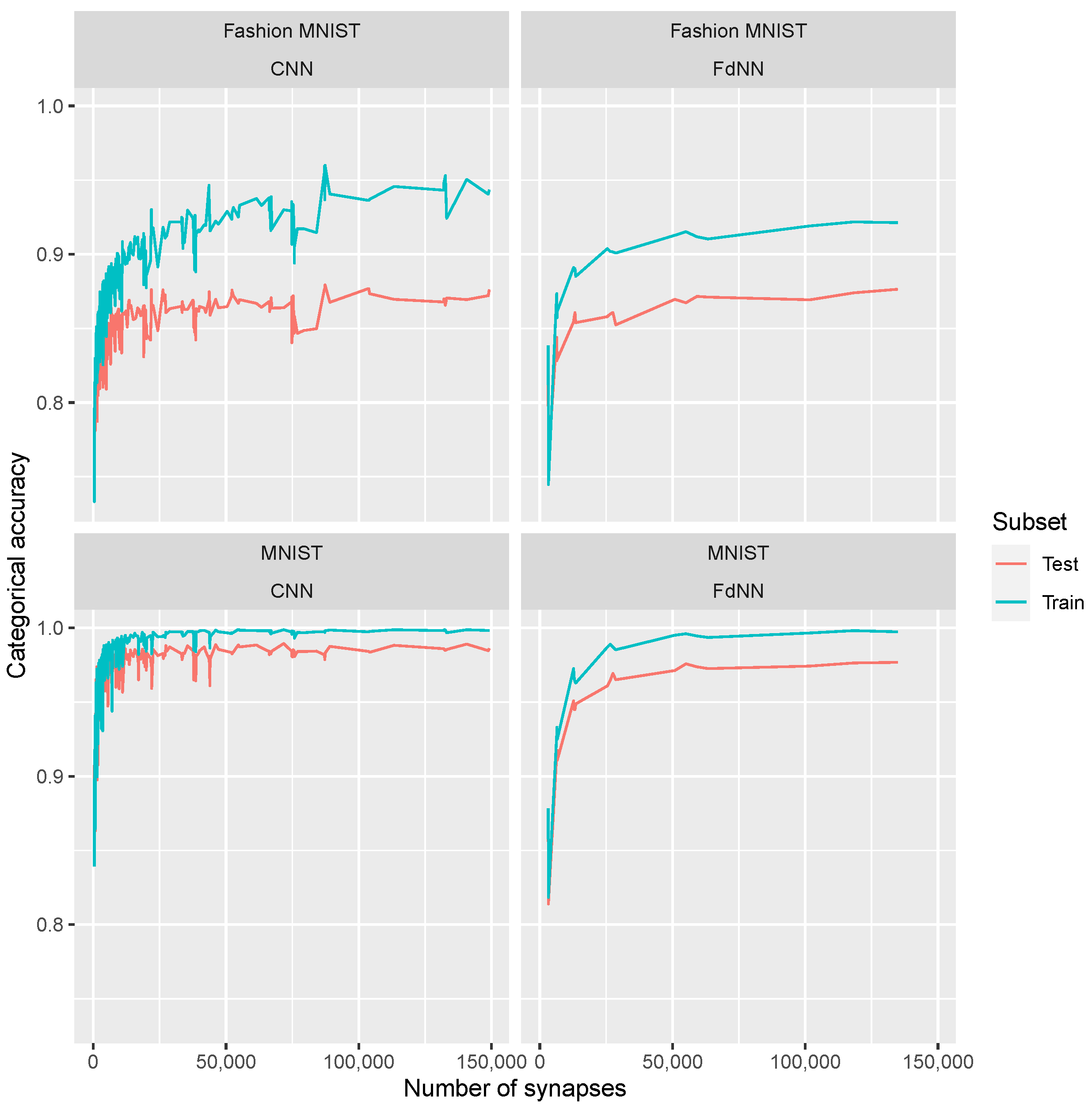
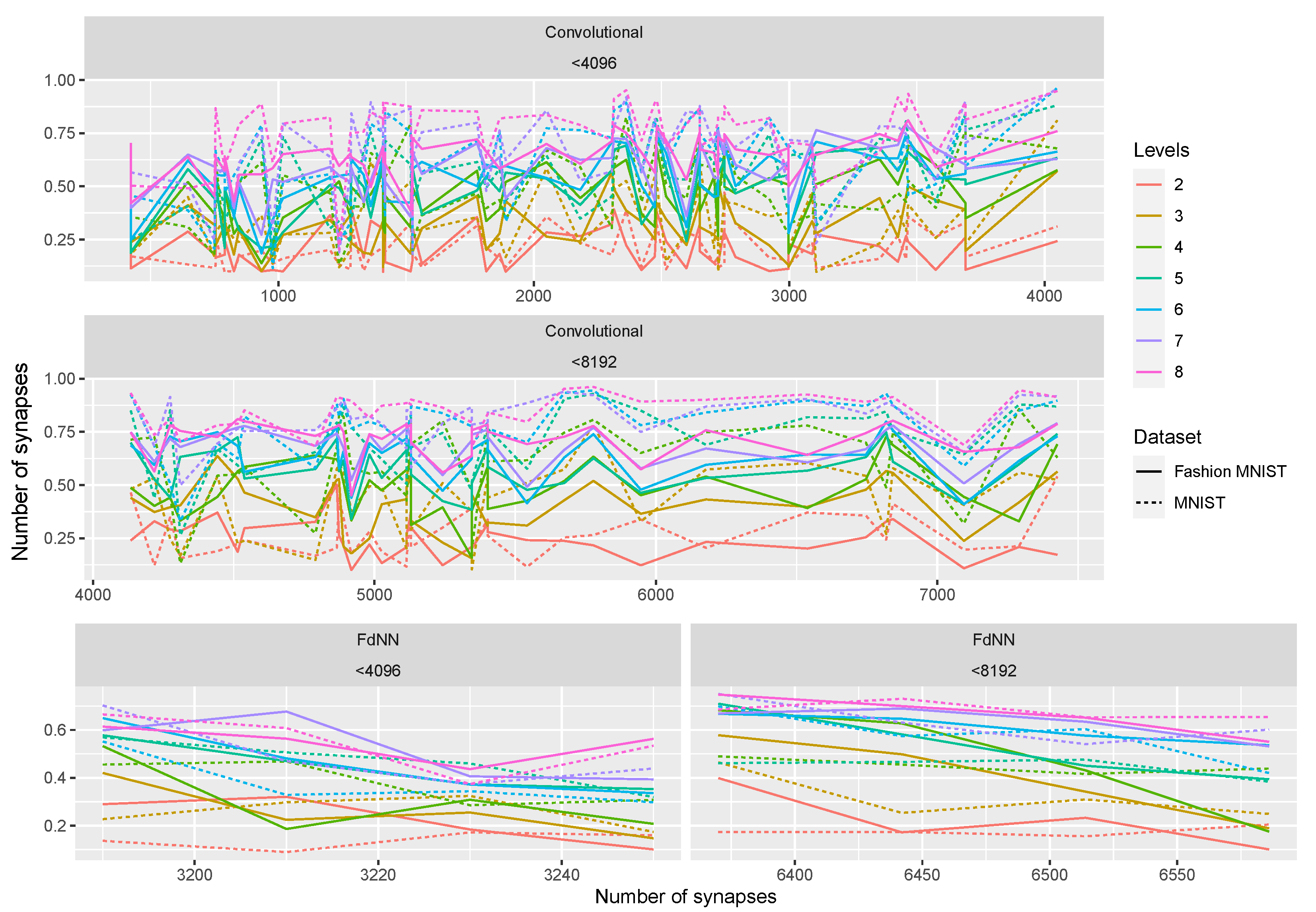
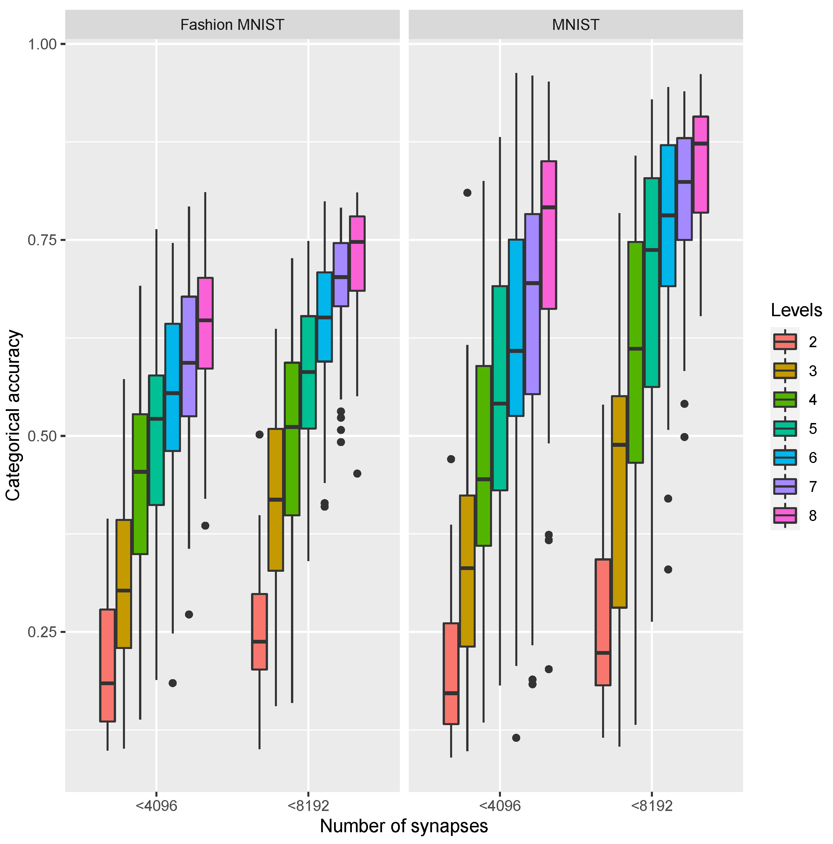
The role of quantization and variability in different types of NNs has been analyzed. The consequences of weight precision reduction have been described previously [18,19]; the variability on the quantization process was tackled from the perspective of device modeling [28], circuit implementation [29] and NN architecture [30]; however, in all these issues there is a long way to go till industrial maturity is reached. In this manuscript, we have characterized the influence of the NN architecture (fully dense/connected or convolutional), the number of synaptic weights (NN size) for different configurations of the NN hidden layers, and the number of memristor quantized conductance levels on the recognition accuracy achieved over different datasets.

The memristor-based array developed to implement all the different NNs proposed is a 4-kbit 1T1R ReRAM array based on $Hf{O}_2$ dielectrics, which show a clear bipolar operation where conductive filaments are made of oxygen vacancies. The multilevel conductance modulation is achieved by using the Incremental Gate Voltage with Verify Algorithm (IGVVA), which can provide any combination of levels between 2 and 8 [31]. We have kept in mind that it has been proven that only a 3-bit precision was needed to correctly encode state-of-the-art networks [18]. This corresponds to the higher number of levels analyzed here. From another viewpoint, quantization could be beneficial to deal with common problems in the NN realm, such as overfitting. We have dealt with all these issues as the manuscript unfolded; in Section 2 the technological features of the devices employed are described, the NN architecture and the basis of the study performed are given in Section 3, finally, the main results and corresponding discussions are explained in Section 4.

2. Experimental Description

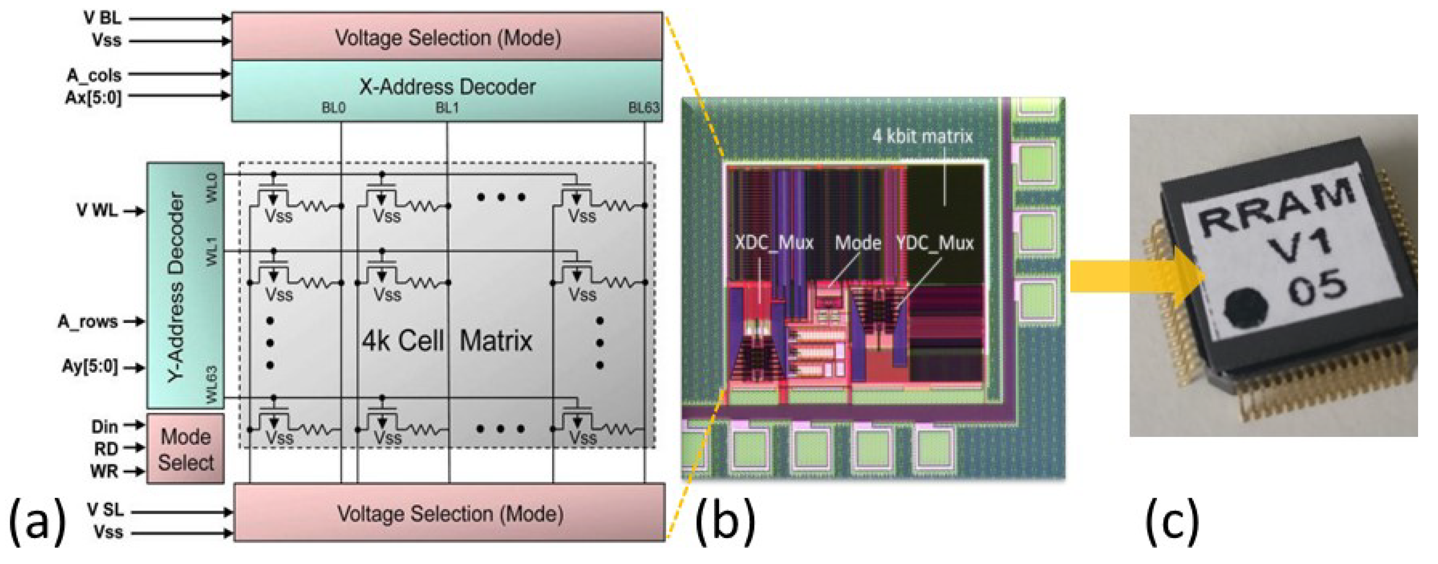
The crossbar arrays utilized in this work are 4-kbit 1T1R ReRAM arrays integrated together with basic circuit periphery and encapsulated in memory chips [32], as shown in Figure 1. Each ReRAM cell is constituted by a NMOS transistor (manufactured in 0.25 $\mathsf{\mu }$m CMOS technology) connected in series to a metal–insulator–metal (MIM) structure placed on the metal line 2 of the CMOS process [29]. The MIM structure consists of a $TiN/Hf{O}_2/Ti/TiN$ stack with 150 nm TiN top and bottom electrode layers deposited by magnetron sputtering, a 7 nm Ti layer (under the TiN top electrode) and an 8 nm $Hf{O}_2$ layer grown by atomic layer deposition (ALD) [33].

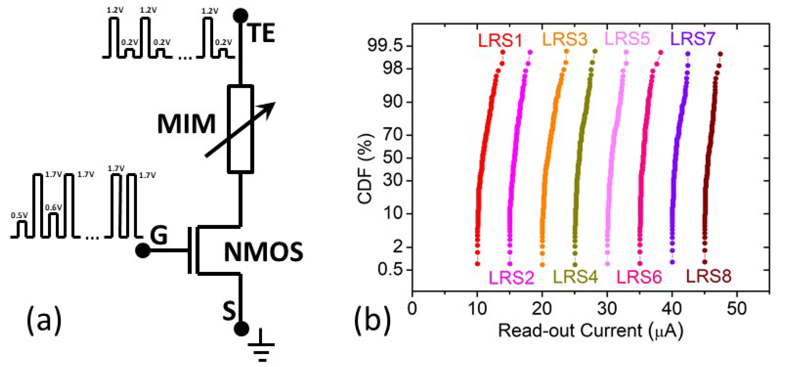
In order to implement the quantized weight values in the NN architectures considered here, a write-verify programming algorithm was employed, namely, the IGVVA. This algorithm, tested on our technology for the first time in [31], keeps constant the pulse amplitude applied on the terminal connected to the top electrode (TE) of the MIM structure during set operations and increases step by step the gate voltage ($V_g$) value until a desired readout (at 0.2 V) current target ($I_{trg}$) is achieved (see Figure 2a). The cumulative distribution functions (CDFs) of the readout currents measured on 128 ReRAM cells for eight different conductive levels are shown in Figure 2b. Therefore, this programming approach provides the right tool to define all different quantization levels tested in this work.

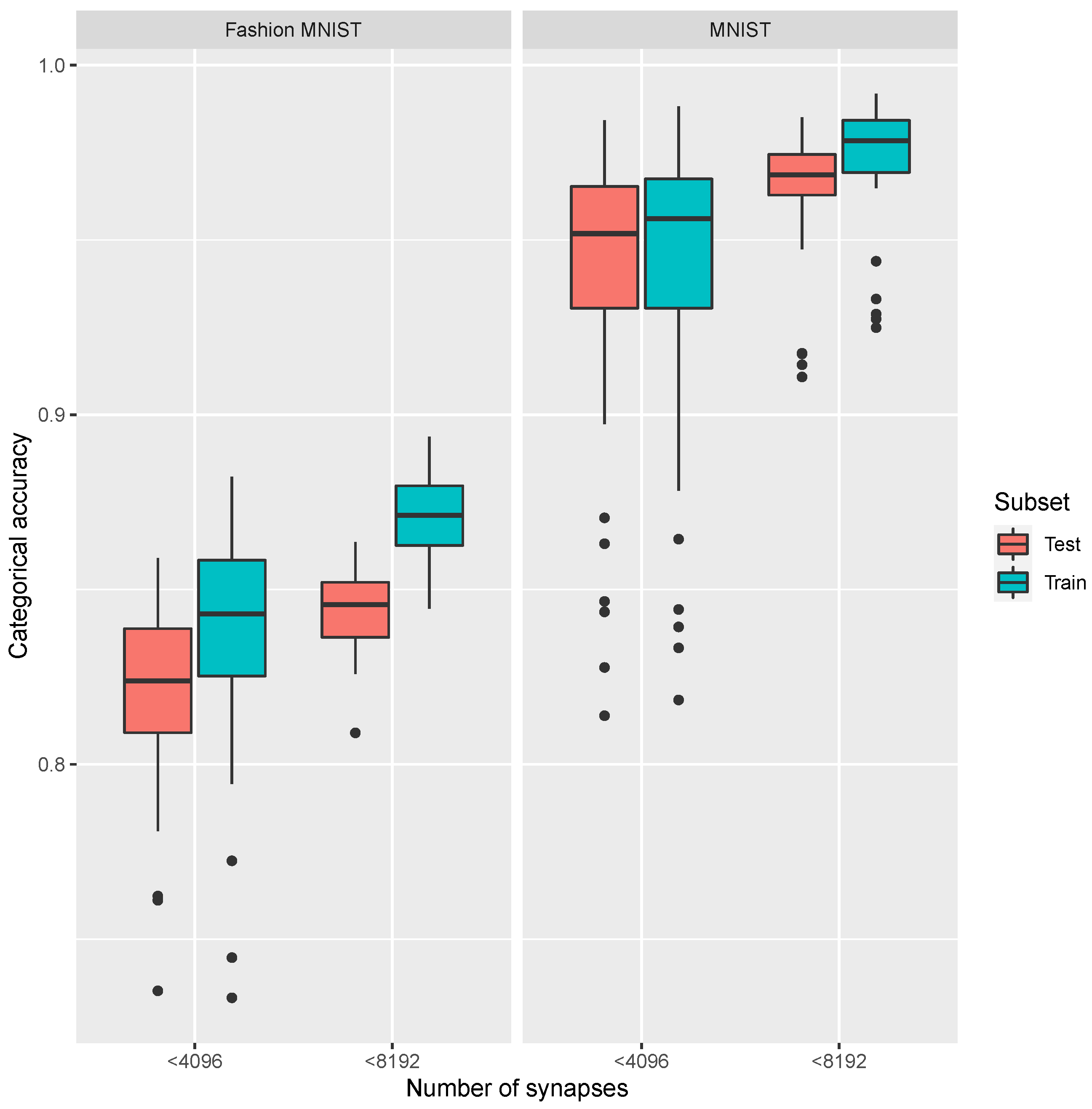
Our arrays exactly contain 4096 cells, so this is the number we have considered in our study as the reference for the number of synaptic weights of the NN analyzed (we have considered mainly one and two arrays). We have studied NNs with a low number of synapses, trying to optimize the NN recognition accuracy and considering the possibility of implementing the NN in this technology and with the crossbar arrays described above.

3. Neural Network Architecture

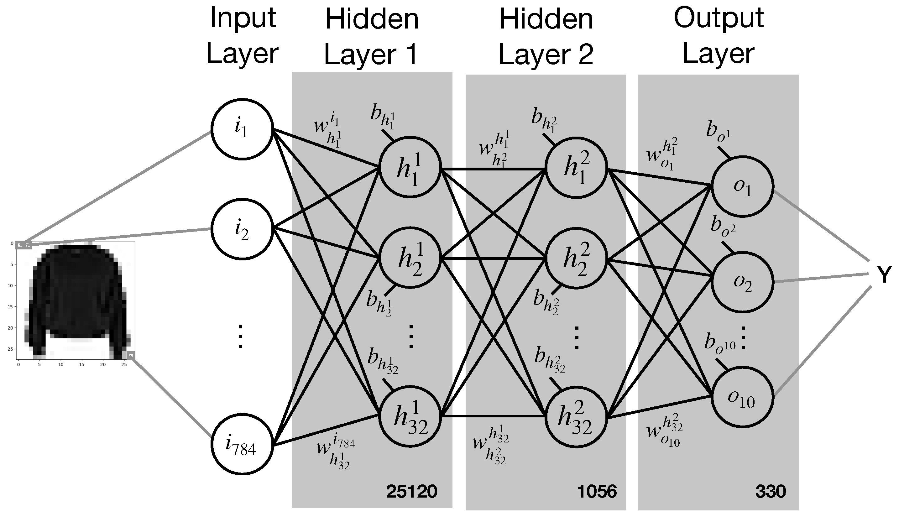
Different architectures have been considered here; in particular, as highlighted above, fully dense and convolutional NNs. In Figure 3, the scheme of FdNN is shown, the number of weights employed in this particular configuration is described. It is clear that if we vary the number of hidden layers, the NN amount of weights can be changed for the study we present below. Notice that deepening in a fully dense NN will highly increase the number of synaptic weights as all units from a layer are connected to all units in the next layer.

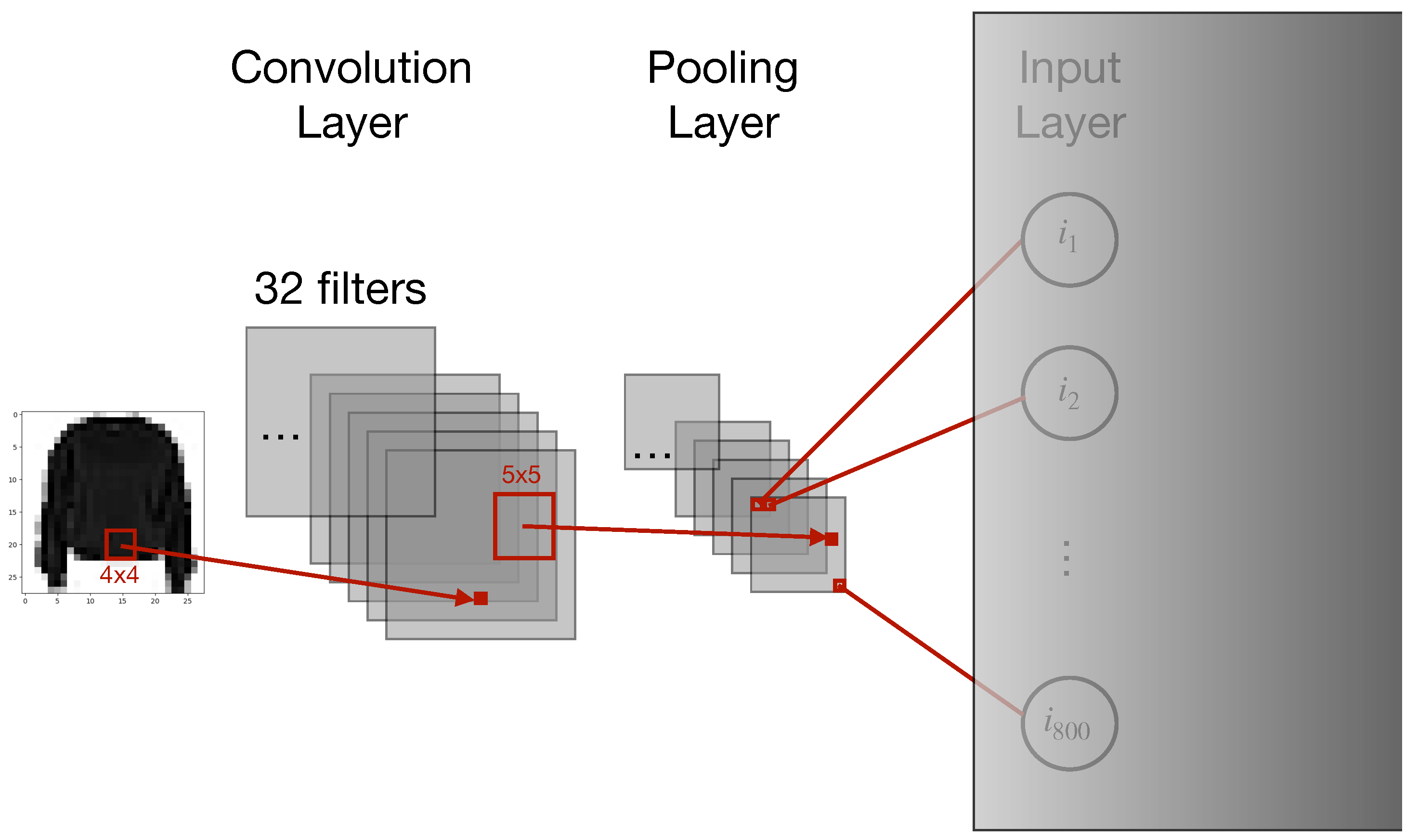
In Figure 4, the architecture of a Convolutional Neural Network (CNN) is described. They are widely employed for image recognition issues in perception activities; at this task, they perform a fast and highly parallel data processing [34]. In a CNN, preprocessing layers are used before the final FdNN. These special layers are called convolution layers and pooling layers. The former apply a set of filters to the input data in order to create maps that summarize the presence of detected features. The latter down-sample those features, reducing the number of units needed to process the input data. We have employed this somewhat general scheme to build the CNN architecture following a previous work [30], to be able to change the number of synaptic weights for our study.

For both types of networks we have assumed a deep NN approach (we assume “deep” as the use of two or more hidden layers in fully dense NNs; CNNs are considered always deep) since these type of NNs have shown the correct features to fulfill a high degree of accuracy in learning complex and massive datasets [35,36,37,38]. We have focused our study in the influence of the number of synaptic weights on the accuracy of the networks. To do so, we have changed the network architecture using the NNs explained above as a starting point and increasing the number of hidden layers, neurons per layer, number of filters, etc. The motivation behind this analysis stands on the limited size of the available ReRAM crossbar arrays, namely, 4096 1T1R cells in our technology. This is a first approach in this type of study, based on the NN size, calculated in terms of the number of the most representative elements. There is still the possibility of using several crossbar arrays on a tiled architecture in order to provide a larger number of synaptic devices for the NN implementation. However, it is important to highlight that the optimization process of the hardware-based NN stands upon the use of the lowest number of crossbar arrays, obtaining a reasonable accuracy. The tiled structure design details are out of the scope of the study presented here. At this point, notice that our approach is much different to the conventional studies performed in the context of software engineering, where gigantic NN are considered to achieve recognition accuracy top figures. In this respect, we make clear that, in the latter context, obviously, the state of the art for the NN under consideration is different to what we obtain here [39,40].

For our study, we have used two datasets: the MNIST [41] and Fashion MNIST [42]. The MNIST image dataset [41] consist of 70,000 grayscale pixel images; they represent handwritten digits (labeled in the interval $[0,9]$), divided into a training set of size 60,000 and a test set of size 10,000. The Fashion MNIST dataset [42] has 70,000 28 × 28 grayscale images in 10 classes (T-shirt/top, Trouser, Pullover, Dress, Coat, Sandal, Shirt, Sneaker, Bag and Ankle boot). The training set has 60,000 images and a test set 10,000 (see Figure 7 in [30]), this dataset is more complex to learn than the original MNIST, and for image recognition purposes, it represents a more real-world approach [42].

For each dataset, we have run several simulation experiments for the two types of NNs described above. The NNs were trained using the default parameter values of the keras/tensorflow implementation (some hyperparameters employed were linked to the stochastic gradient descend algorithm with $learningrate=0.1$ and $momentum=0.9$). We utilized the categorical accuracy as the comparison metric. It obtains the relative frequency in which the prediction matches the labeled data, and this frequency is then returned as categorical accuracy [43,44]. The main goal of this work is to study the effect of synaptic weight quantization in hardware neural networks with different configurations that come up because of the number of synapses constraints imposed by the use of memristor-based arrays of 4-kbit 1T1R cells. Although we have not performed multiple simulation runs for all the NN analyzed, we have considered a representative example (a CNN with three convolution layers, 16 filters, 2 × 2 pooling layers and a hidden layer with 32 neurons in the fully dense section of the network) and analyzed the random deviations among different simulations. We obtained an average accuracy of 0.909 and standard deviation of 0.035 for 10 simulation runs. In this respect, we expect, taking into consideration the similitude of the different NN architectures, that the results within our work could be accurate within a margin of $5\%$.

4. Results and Discussion

4.1. Full Precision

As a first step in the analysis, we neglected synaptic weight quantization. The NN accuracy in weight full precision was analyzed as shown in Figure 5 for CNN and FdNN architectures using up to 150,000 synapses.

We can see that as the number of synapses used in both FdNN and CNN increases, the accuracy approaches optimal values. This behavior is similar in the train and test subsets, although test results are always lower than in the train case due to probable overfitting [45]. The FdNN seems to have a slower improvement for the MNIST dataset when the number of synapses increases compared to CNN. As expected, a deep NN is (therefore a high number of synaptic weights) needed to obtain a reasonable accuracy; nevertheless, this means a high cost in the hardware implementation due to the great number of memristors, and therefore the number of crossbar arrays, required.

In order to clarify the correlation between NN accuracy and different aspects of our study, the following calculations were made.

Table 1. Spearman’s correlation test between the number of synapses and the categorical accuracy for each simulation experiment.

Experiment		FdNN		CNN
Dataset	Subset	p-Value	$\mathbf{\rho }$	p-Value	$\mathbf{\rho }$
MNIST	Train	2.64 × 10−6	0.96	<2.2 × 10−16	0.92
MNIST	Test	2.16 × 10−14	0.97	<2.2 × 10−16	0.81
Fashion MNIST	Train	2.74 × 10−6	0.95	<2.2 × 10−16	0.93
Fashion MNIST	Test	3.13 × 10−6	0.93	<2.2 × 10−16	0.80

shows the correlation tests performed to describe the link between the categorical accuracy and the number of synapses. As can be seen, there is a clear relation between these magnitudes in all the simulation experiments. In all cases the Spearman’s correlation test reports a p-value below $0.05$. Spearman’s correlation coefficient $\rho$ is a nonparametric statistical measure of the strength of a monotonic relationship between two variables, where values closer to 0 indicate a very weak correlation, while values closer to ±1 indicate a very strong correlation. Statistical significance is assessed in this test, as well in all the following tests performed, obtaining a p-value that will allow us to distinguish statistically relevant observations from those likely to occur by chance.

A parallel study shows us the link between the NN accuracy and the number of neurons in the hidden layers (see

Table 2. Spearman’s correlation test between number of hidden units and categorical accuracy for each simulation experiment.

Experiment		FdNN		CNN
Dataset	Subset	p-Value	$\mathbf{\rho }$	p-Value	$\mathbf{\rho }$
MNIST	Train	<2.2 × 10−16	0.99	<2.2 × 10−16	0.53
MNIST	Test	<2.2 × 10−16	0.98	<2.2 × 10−16	0.57
Fashion MNIST	Train	<2.2 × 10−16	0.99	1.63 × 10−11	0.41
Fashion MNIST	Test	6.53 × 10−12	0.95	3.63 × 10−10	0.38

). The correlation is clear in this case, however, the $\rho$ for CNNs is much lower that in the FdNNs case, indicating a weaker connection of the magnitudes at stake.

Concerning CNN, the correlation tests are shown in

Table 3. Spearman’s correlation test between number of convolutional layers/number of filters/size of pooling layers and categorical accuracy for each experiment.

Experiment		Conv. Layers		Filters		Pool. Size
Dataset	Subset	p-Value	$\mathbf{\rho }$	p-Value	$\mathbf{\rho }$	p-Value	$\mathbf{\rho }$
MNIST	Train	0.1879	0.084	1.17 × 10−13	0.448	1.15 × 10−10	−0.394
MNIST	Test	0.0041	0.182	7.08 × 10−11	0.399	1.05 × 10−9	−0.375
Fashion MNIST	Train	0.2237	−0.077	3.33 × 10−14	0.457	3.38 × 10−9	−0.364
Fashion MNIST	Test	0.0005	−0.219	6.46 × 10−9	0.358	5.41 × 10−5	−0.253

. The number of convolutional layers are not correlated with the NN accuracy for the train subsets; however, it seems to be a weak correlation for the test subset. Regarding the number of filters, there is a statistically significant positive correlation; while for the size of the pooling layers, there is a statistically significant negative correlation. These outcomes are not surprising since the bigger the size of a pooling layer, the higher the reduction in the input data size; also, the higher the number of filters generally helps to identify important features of the input data, thus increasing the overall accuracy.

We also analyzed the behavior of the different neural network approaches using architectures with less than 4096 synapses (1 crossbar array) and with a number of synapses between 4096 and 8192 (two crossbar arrays). This strategy makes sense taking into consideration the architectural blocks of our ICs; i.e., arrays of 4096 1T-1R ReRAM cells; although it is clear that each NN architecture would need a particular hardware implementation. In this respect, we would consider one, two or multiples of sets of 4096 synapses. It can be seen that the accuracy obtained is higher when using higher number of synapses. However, some specific architectures may partially compensate it. For FdNN we considered hidden layers, in the CNN case we accounted for several convolutional layers.

A summary of the results obtained in the previous figures is better explained in Figure 6. In addition to the difference between both datasets, the results validate what was expected: 8192 synapses work better than 4096 synapses, regardless of the type of NN used.

4.1.1. Less Than 4096 Synapses

To build FdNNs using less than 4096 synapses we require architectures with a low number of hidden units (see

Table 4. Architectures for FdNN with less than 4096 synapses.

			MNIST		Fashion MNIST
Hidden Layers	Hidden Units	Synapses	Train	Test	Train	Test
1	4	3190	0.88	0.87	0.84	0.81
2	4	3210	0.84	0.85	0.79	0.79
3	4	3230	0.83	0.83	0.77	0.76
4	4	3250	0.82	0.81	0.74	0.76

). We employed four neurons per layer, obtaining most of the lowest accuracy results compared to the rest of the simulation experiments (recall Figure 7).

For CNNs, different architectures are analyzed, some of them using as low as 422 synapses. The best neural network with less than 4096 synapses is a CNN with 2 convolutional layers, eight filters, pooling size matrix of $2\times 2$ and 16 hidden units, achieving an accuracy of $0.988$ in training and $0.984$ in test for the MNIST dataset and $0.882$ in training and $0.846$ in test for the Fashion MNIST dataset.

4.1.2. Between 4096 and 8192 Synapses

FdNNs using between 4096 and 8192 synapses greatly improve the ones using less than 4096 synapses (see Figure 6 and

Table 5. Architectures for FdNN with a number of synapses between 4096 and 8192.

Hidden Layers	Hidden Units	Synapses	Train	Test
1	8	6370	0.927	0.914
2	8	6442	0.933	0.917
3	8	6514	0.929	0.918
4	8	6586	0.925	0.911

). To check the statistical significance of these results we applied a Kruskal–Wallis Rank Sum Test, which is a non-parametric test used to assess whether two or more samples (<4096 vs. between 4096 and 8192) originate from the same distribution. Results indicate that, for both datasets and in training and test, there is a statistically significant difference (

Table 6. Kruskal–Wallis Rank Sum Test between the accuracy in NNs with less than 4096 synapses and with a number of synapses between 4096 and 8192.

Experiment		FdNN	CNN
Dataset	Subset	p-Value	p-Value
MNIST	Train	0.021	9.54 × 10−10
MNIST	Test	0.021	1.79 × 10−7
Fashion MNIST	Train	0.021	3.31 × 10−10
Fashion MNIST	Test	0.021	2.52 × 10−8

).

For CNNs there are multiple architectures found in between 4096 and 8192 synapses (see the top 10 in

Table 7. Top 10 architectures for CNN with a number of synapses in between 4096 and 8192.

Conv.	Filters	Pooling	Hidden	Synapses	MNIST		Fashion MNIST
Layers		Size	Units		Train	Test	Train	Test
1	16	4	8	4866	0.985	0.974	0.883	0.857
1	8	4	16	4874	0.984	0.977	0.887	0.858
2	16	3	32	4890	0.989	0.982	0.880	0.847
2	16	2	8	5778	0.990	0.981	0.892	0.853
2	16	2	8	5778	0.990	0.981	0.892	0.853
1	16	5	16	6746	0.989	0.977	0.892	0.862
1	32	5	8	6818	0.988	0.975	0.893	0.864
1	8	5	32	6842	0.984	0.971	0.894	0.863
2	16	3	64	7290	0.992	0.985	0.885	0.858
2	8	2	32	7426	0.990	0.981	0.891	0.859

). The results show that the accuracy when using more than 4096 synapses increases. Once again, the Kruskal–Wallis Rank Sum Tests performed indicate that for both datasets and for both training and test sets, using CNNs, there is a difference in terms of statistical significance (see Table 6), meaning that the results obtained are not likely to occur by chance.

The best NN with a number of synapses between 4096 and 8192 is a CNN with 2 convolutional layers, eight filters, pooling size matrix of $3\times 3$ and 64 hidden units, achieving an accuracy of $0.992$ in training and $0.985$ in test for the MNIST dataset, and also a CNN with one convolutional layer, 32 filters, pooling size matrix of $5\times 5$ and eight hidden units, achieving a $0.883$ in training and $0.864$ in test for the Fashion MNIST dataset.

4.2. Analysis Assuming Quantized Synaptic Weights

The synaptic weights are quantized following a conductance multilevel approach as highlighted in Refs. [29,30] and along with the experimental results described above, see Figure 2b. In line with previous developments, we have studied the correlation between the NN accuracy and the number of synapses for different quantization levels, (see

Table 8. Mean values for Spearman’s correlation test between the NN number of synapses and the categorical accuracy for each simulation experiment regardless of the quantization level.

	FdNN		CNN
Dataset	p-Value	$\mathbf{\rho }$	p-Value	$\mathbf{\rho }$
MNIST	2.639 × 10−6	0.92	6.05 × 10−18	0.65
Fashion MNIST	0.0007	0.83	9.28 × 10−18	0.69

).

In the same manner, the correlation between the number of hidden neurons and the categorical accuracy has been studied for different quantization levels. The Spearman’s correlation test in

Table 9. Mean values for Spearman’s correlation test between number of hidden units and categorical accuracy for each simulation experiment regardless of the quantization level.

	FdNN		CNN
Dataset	p-Value	$\mathbf{\rho }$	p-Value	$\mathbf{\rho }$
MNIST	9.88 × 10−11	0.95	8.00 × 10−17	0.62
Fashion MNIST	5.85 × 10−5	0.89	5.62 × 10−15	0.58

indicates that there is significant statistical difference (p-value < 0.05) between the number of synapses and the accuracy for both datasets for all levels of precision studied.

We analyze in

Table 10. Spearman’s correlation test between the number of convolutional layers/number of filters/size of pooling layers and the categorical accuracy for each experiment using quantization levels between 2 and 8.

		conv. Layers		Filters		Pool. Size
Dataset	Levels	p-Value	$\mathbf{\rho }$	p-Value	$\mathbf{\rho }$	p-Value	$\mathbf{\rho }$
MNIST	2	0.508	0.042	0.455	−0.048	0.345	0.060
MNIST	3	0.873	−0.010	4.82 × 10−24	0.584	8.08 × 10−6	−0.279
MNIST	4	0.008	0.168	0.0003	0.226	9.41 × 10−6	−0.277
MNIST	5	0.010	0.163	0.002	0.196	2.87 × 10−6	−0.292
MNIST	6	0.0008	0.212	0.032	0.136	2.07 × 10−6	−0.296
MNIST	7	0.0006	0.215	0.001	0.207	6.60 × 10−7	−0.309
MNIST	8	0.016	0.153	0.0003	0.229	2.30 × 10−5	−0.265
Fashion MNIST	2	0.508	0.042	0.455	−0.048	0.345	0.060
Fashion MNIST	3	0.873	−0.010	4.82 × 10−24	0.584	8.08 × 10−6	−0.279
Fashion MNIST	4	1.99 × 10−16	−0.491	0.605	0.033	0.155	0.090
Fashion MNIST	5	4.84 × 10−6	−0.286	0.0006	0.217	0.465	−0.047
Fashion MNIST	6	0.0004	−0.221	0.0003	0.227	0.128	−0.097
Fashion MNIST	7	0.0006	−0.217	2.75 × 10−5	0.263	0.034	−0.134
Fashion MNIST	8	0.00008	−0.248	3.32 × 10−5	0.260	0.016	−0.153

the possible correlation between the categorical accuracy and three variables in CNNs: the number of convolutional layers, the number of filters and the pooling size, taking into account the different datasets and levels from 2 to 8. Results show statistically significant negative correlations in the Fashion MNIST dataset for almost all the simulation experiments performed with different number of convolutional layers, indicating that this feature is relevant to the NN outcome. On the contrary, the MNIST dataset shows no correlation between the number of convolutional layers and the NN accuracy. This is probably due to the fact that MNIST dataset is less complex than the Fashion MNIST dataset, showing no impact in the categorical accuracy when the number of convolutional layers is altered. The number of filters, however, present significant and small positive correlation values for both datasets, specially when the number of levels is high. This behavior implies that the number of filters is somewhat relevant to obtaining better accuracy levels. Finally, the pooling size present a significant and small negative correlation for levels greater than 2 in the MNIST dataset but no significant correlation for the Fashion MNIST dataset. In this respect, an increase in the pooling size reduces the number of neurons and thus negatively affects the NN accuracy.

In

Table 11. Kruskal–Wallis Rank Sum Test between CNNs comparing results obtained by using less than 4096 synapses and between 4096 and 8192 synapses for each simulation experiment using quantization levels between 2 and 8.

Experiment		FdNN	CNN
Dataset	Levels	p-Value	p-Value
MNIST	2	0.08	1.34 × 10−3
MNIST	3	0.39	2.40 × 10−3
MNIST	4	0.56	3.19 × 10−4
MNIST	5	0.77	.37 × 10−5
MNIST	6	0.04	4.07 × 10−6
MNIST	7	0.15	7.02 × 10−6
MNIST	8	0.08	2.50 × 10−4
Fashion MNIST	2	1.00	3.24 × 10−2
Fashion MNIST	3	0.25	5.14 × 10−4
Fashion MNIST	4	0.39	9.45 × 10−2
Fashion MNIST	5	0.25	2.49 × 10−3
Fashion MNIST	6	0.15	3.19 × 10−4
Fashion MNIST	7	0.25	1.57 × 10−5
Fashion MNIST	8	0.15	9.75 × 10−6

, we tested if the results obtained using less than 4096 synapses and using between 4096 and 8192 differ with a high statistical significance. To do so, we applied a Kruskal–Wallis Rank Sum Test with both samples, particularized to each dataset, number of levels and NN type. The results show that for FdNN, the difference between the samples were probably random, while for CNN there is an actual difference supported by the statistical analysis. We simulated reducing the synaptic weights floating point precision from 32 bits to a range of limited precision levels, between 2 and 8 levels (i.e., 1 to 3 bits) using the test subsets for both datasets. Figure 8 shows the behavior of the limited precision in both datasets.

Comparing Figure 8 to Figure 7, we can see that the difference between MNIST and Fashion MNIST fades. On the one hand, for the FdNN, the maximum precision drops significantly, achieving no more than 75% of accuracy; on the other hand, CNNs can obtain a similar precision to the original floating point version when the number of levels is high enough. The accuracy obtained by using CNNs does not seem to follow a clear trend as the number of synapses increases. This is due to the fact that there are several and quite disimilar CNN architectures using a similar number of synapses (recall Table 7 and

Table 12. Top 10 architectures for CNN with less than 4096 synapses.

Conv.	Filters	Pooling	Hidden	Synapses	MNIST		Fashion MNIST
Layers		Size	Units		Train	Test	Train	Test
1	8	5	8	1778	0.968	0.966	0.861	0.841
1	16	6	8	2306	0.973	0.968	0.865	0.847
1	8	4	8	2482	0.978	0.972	0.875	0.843
2	16	3	8	3090	0.980	0.975	0.872	0.847
2	16	4	32	3354	0.974	0.965	0.871	0.844
2	8	3	64	3426	0.982	0.978	0.867	0.841
1	16	5	8	3458	0.977	0.965	0.880	0.858
1	8	5	16	3466	0.978	0.970	0.879	0.859
2	16	3	16	3690	0.986	0.982	0.881	0.848
2	8	2	16	4050	0.988	0.984	0.882	0.846

), showing how each distinct architecture positively or negatively affects the final NN outcome. In the case of FdNN, the trend is smoother, since the number of synapses is directly controlled by the number of hidden units and hidden layers. When a new hidden layer is proposed, the number of neurons increases creating small peaks (shown in the lower boxes of the plot). If the number of levels is particularly small, the accuracy of the network is highly affected since the NN architecture cannot compensate it. Additionally, notice that the number of possible architectures using FdNN with small amount of neurons is smaller than the number of options that can be achieved with CNN architectures, mainly due to the pooling layers, that reduce the number of synapses.

A deeper study is shown in Figure 9, where it is easier to spot the differences between precision level and accuracy. From Table 11, we can infer that there is a clear statistical difference between using less than 4096 synapses compared to using between 4096 and 8192 when working with CNNs in both datasets. On the contrary, when working with FdNN, only MNIST dataset with six levels of precision achieves a p-value < 0.05.

5. Conclusions

We have analyzed the architecture of neural networks for hardware implementation by means of simulation experiments to assess the connection between the NN number of synapses and the accuracy. Both fully dense and convolutional neural networks were studied by changing the architecture configurations, and mostly the NN size in terms of the number of synapses and of hidden layer neurons. The results show that CNNs work better when the number of synapses to be used is limited. Additionally, when the precision is restricted to a low number of levels (that would mean a multilevel approach for the memristors in the crossbar arrays), the NN accuracy drops off significantly as the number of synapses is reduced. Therefore, in order to obtain good results we need a trade-off between the number of synapses and the accuracy. To take advantage of this trade-off, the CNN architecture must be carefully devised, balancing the parameters used in the different layer components. We also noticed that different datasets would need specific architectures according to their complexity. When the number of synaptic weight levels is as low as 2, the NN accuracy obtained is low; therefore, in this case, instead of just discretizing the synaptic weights of a full precision NN, an approach based on binary neural networks could be the way to go [46]. As it was shown, due to the number of variables that can be changed in the optimization of a NN hardware implementation, a specific solution has to be worked in each case, in terms of synaptic weight levels, NN architecture, etc.

References

1. Tsur, E.E. Neuromorphic Engineering; CRC Press: Boca Raton, FL, USA, 2021. [Google Scholar]
2. Tang, J.; Yuan, F.; Shen, X.; Wang, Z.; Rao, M.; He, Y.; Sun, Y.; Li, X.; Zhang, W.; Li, Y.; et al. Bridging Biological and Artificial Neural Networks with Emerging Neuromorphic Devices: Fundamentals, Progress, and Challenges. Adv. Mater. 2019, 31, 1902761. [Google Scholar] [CrossRef] [PubMed]
3. Dhar, P. The carbon impact of artificial intelligence. Nat. Mach. Intell. 2020, 2, 423–425. [Google Scholar] [CrossRef]
4. Ben Varkey, B.E.A. Neurogrid: A mixed-analog-digital multichip system for large-scale neural simulations. Proc. IEEE 2014, 102, 699–716. [Google Scholar]
5. Furber, S.B.E.A. TheSpiNNakerproject. Proc. IEEE 2014, 102, 652–665. [Google Scholar] [CrossRef]
6. DeBole, M.V.; Taba, B.; Amir, A.; Akopyan, F.; Andreopoulos, A.; Risk, W.P.; Kusnitz, J.; Otero, C.O.; Nayak, T.K.; Appuswamy, R.; et al. TrueNorth: Accelerating From Zero to 64 Million Neurons in 10 Years. Computer 2019, 52, 20–29. [Google Scholar] [CrossRef]
7. Davies, M.E.A. Loihi: A neuromorphic many core processor with on-chip learning. IEEE Macro 2018, 38, 82–99. [Google Scholar] [CrossRef]
8. Lanza, M.; Wong, H.S.P.; Pop, E.; Ielmini, D.; Strukov, D.; Regan, B.C.; Larcher, L.; Villena, M.A.; Yang, J.J.; Goux, L.; et al. Recommended Methods to Study Resistive Switching Devices. Adv. Electron. Mater. 2019, 5, 1800143. [Google Scholar] [CrossRef] [Green Version]
9. Krestinskaya, O.; James, A.P.; Chua, L.O. Neuromemristive Circuits for Edge Computing: A Review. IEEE Trans. Neural Netw. Learn. Syst. 2020, 31, 4–23. [Google Scholar] [CrossRef] [Green Version]
10. Lanza, M.; Waser, R.; Ielmini, D.; Yang, J.J.; Goux, L.; Suñe, J.; Kenyon, A.J.; Mehonic, A.; Spiga, S.; Rana, V.; et al. Standards for the Characterization of Endurance in Resistive Switching Devices. ACS Nano 2021, 15, 17214–17231. [Google Scholar] [CrossRef] [PubMed]
11. Hui, F.; Liu, P.; Hodge, S.A.; Carey, T.; Wen, C.; Torrisi, F.; Galhena, D.T.L.; Tomarchio, F.; Lin, Y.; Moreno, E.; et al. In Situ Observation of Low-Power Nano-Synaptic Response in Graphene Oxide Using Conductive Atomic Force Microscopy. Small 2021, 17, 2101100. [Google Scholar] [CrossRef]
12. Jeong, H.; Shi, L. Memristor devices for neural networks. J. Phys. D Appl. Phys. 2018, 52, 023003. [Google Scholar] [CrossRef]
13. Prezioso, M.; Merrikh-Bayat, F.; Hoskins, B.; Adam, G.; Likharev, K.; Strukov, D. Training and operation of an integrated neuromorphic network based on metal-oxide memristors. Nature 2015, 521, 7550. [Google Scholar] [CrossRef] [PubMed] [Green Version]
14. Xia, Q.; Berggren, K.K.; Likharev, K.; Strukov, D.B.; Jiang, H.; Mikolajick, T.; Querlioz, D.; Salinga, M.; Erickson, J.; Pi, S.; et al. Roadmap on emerging hardware and technology for machine learning. Nanotechnology 2020, 32, 012002. [Google Scholar]
15. Yan, B.; Li, B.; Qiao, X.; Xue, C.X.; Chang, M.F.; Chen, Y.; Li, H.H. Resistive Memory-Based In-Memory Computing: From Device and Large-Scale Integration System Perspectives. Adv. Intell. Syst. 2019, 1, 1900068. [Google Scholar] [CrossRef] [Green Version]
16. Sebastian, A.; Le Gallo, M.; Khaddam-Aljameh, R.; Eleftheriou, E. Memory devices and applications for in-memory computing. Nat. Nanotechnol. 2020, 15, 529–543. [Google Scholar] [CrossRef]
17. Hu, X.; Duan, S.; Chen, G.; Chen, L. Modeling affections with memristor-based associative memory neural networks. Neurocomputing 2017, 223, 129–137. [Google Scholar] [CrossRef]
18. Zheng, N.; Mazumder, P. Learning in Energy-Efficient Neuromorphic Computing: Algorithm and Architecture Co-Design; Wiley: West Sussex, UK, 2019. [Google Scholar]
19. Zhang, Y.; Cui, M.; Shen, L.; Zeng, Z. Memristive Quantized Neural Networks: A Novel Approach to Accelerate Deep Learning On-Chip. IEEE Trans. Cybern. 2019, 51, 1875–1887. [Google Scholar] [CrossRef] [PubMed]
20. Yu, S.; Jiang, H.; Huang, S.; Peng, X.; Lu, A. Computing-in-memory chips for deep learning: Recent trends and prospects. IEEE Circuits Syst. Mag. 2021, 21, 31–56. [Google Scholar] [CrossRef]
21. Aldana, S.; Pérez, E.; Jiménez-Molinos, F.; Wenger, C.; Roldán, J.B. Kinetic Monte Carlo analysis of data retention in Al:HfO2-based resistive random access memories. Semicond. Sci. Technol. 2020, 35, 115012. [Google Scholar] [CrossRef]
22. Villena, M.; Roldan, J.; Jimenez-Molinos, F.; Miranda, E.; Suñé, J.; Lanza, M. SIM2RRAM: A physical model for RRAM devices simulation. J. Comput. Electron. 2017, 16, 1095–1120. [Google Scholar] [CrossRef]
23. Pérez, E.; Maldonado, D.; Acal, C.; Ruiz-Castro, J.; Alonso, F.; Aguilera, A.; Jiménez-Molinos, F.; Wenger, C.; Roldán, J. Analysis of the statistics of device-to-device and cycle-to-cycle variability in TiN/Ti/Al:HfO2/TiN RRAMs. Microelectron. Eng. 2019, 214, 104–109. [Google Scholar] [CrossRef]
24. Roldán, J.B.; Alonso, F.J.; Aguilera, A.M.; Maldonado, D.; Lanza, M. Time series statistical analysis: A powerful tool to evaluate the variability of resistive switching memories. J. Appl. Phys. 2019, 125, 174504. [Google Scholar] [CrossRef]
25. Acal, C.; Ruiz-Castro, J.; Aguilera, A.; Jiménez-Molinos, F.; Roldán, J. Phase-type distributions for studying variability in resistive memories. J. Comput. Appl. Math. 2019, 345, 23–32. [Google Scholar] [CrossRef]
26. Chen, J.; Wu, H.; Gao, B.; Tang, J.; Hu, X.S.; Qian, H. A Parallel Multibit Programing Scheme With High Precision for RRAM-Based Neuromorphic Systems. IEEE Trans. Electron Devices 2020, 67, 2213–2217. [Google Scholar] [CrossRef]
27. Wenger, C.; Zahari, F.; Mahadevaiah, M.K.; Pérez, E.; Beckers, I.; Kohlstedt, H.; Ziegler, M. Inherent Stochastic Learning in CMOS-Integrated HfO2 Arrays for Neuromorphic Computing. IEEE Electron Device Lett. 2019, 40, 639–642. [Google Scholar] [CrossRef]
28. Pérez-Bosch Quesada, E.; Romero-Zaliz, R.; Pérez, E.; Kalishettyhalli Mahadevaiah, M.; Reuben, J.; Schubert, M.A.; Jiménez-Molinos, F.; Roldán, J.B.; Wenger, C. Toward Reliable Compact Modeling of Multilevel 1T-1R RRAM Devices for Neuromorphic Systems. Electronics 2021, 10, 645. [Google Scholar] [CrossRef]
29. Pérez, E.; Pérez-Ávila, A.J.; Romero-Zaliz, R.; Mahadevaiah, M.K.; Pérez-Bosch Quesada, E.; Roldán, J.B.; Jiménez-Molinos, F.; Wenger, C. Optimization of Multi-Level Operation in RRAM Arrays for In-Memory Computing. Electronics 2021, 10, 1084. [Google Scholar] [CrossRef]
30. Romero-Zaliz, R.; Pérez, E.; Jiménez-Molinos, F.; Wenger, C.; Roldán, J.B. Study of Quantized Hardware Deep Neural Networks Based on Resistive Switching Devices, Conventional versus Convolutional Approaches. Electronics 2021, 10, 346. [Google Scholar] [CrossRef]
31. Milo, V.; Anzalone, F.; Zambelli, C.; Pérez, E.; Mahadevaiah, M.K.; Ossorio, Ó.G.; Olivo, P.; Wenger, C.; Ielmini, D. Optimized programming algorithms for multilevel RRAM in hardware neural networks. In Proceedings of the 2021 IEEE International Reliability Physics Symposium (IRPS), Monterey, CA, USA, 21–25 March 2021; pp. 1–6. [Google Scholar] [CrossRef]
32. Zambelli, C.; Grossi, A.; Olivo, P.; Walczyk, D.; Bertaud, T.; Tillack, B.; Schroeder, T.; Stikanov, V.; Walczyk, C. Statistical analysis of resistive switching characteristics in ReRAM test arrays. In Proceedings of the 2014 International Conference on Microelectronic Test Structures (ICMTS), Udine, Italy, 24–27 March 2014; pp. 27–31. [Google Scholar] [CrossRef]
33. Grossi, A.; Perez, E.; Zambelli, C.; Olivo, P.; Miranda, E.; Roelofs, R.; Woodruff, J.; Raisanen, P.; Li, W.; Givens, M.; et al. Impact of the precursor chemistry and process conditions on the cell-to-cell variability in 1T-1R based HfO2 RRAM devices. Sci. Rep. 2018, 8, 11160. [Google Scholar] [CrossRef] [Green Version]
34. Liu, C.; Chen, H.; Wang, S.; Liu, Q.; Jiang, Y.G.; Zhang, D.W.; Liu, M.; Zhou, P. Two-dimensional materials for next-generation computing technologies. Nat. Nanotechnol. 2020, 15, 545. [Google Scholar] [CrossRef]
35. Bashar, A. Survey on Evolving Deep Learning Neural Network Architectures. J. Artif. Intell. Capsul. Netw. 2019, 1, 73–82. [Google Scholar] [CrossRef]
36. Nassif, A.B.; Shahin, I.; Attili, I.; Azzeh, M.; Shaalan, K. Speech recognition using deep neural networks: A systematic review. IEEE Access 2019, 7, 19143–19165. [Google Scholar] [CrossRef]
37. Dhillon, A.; Verma, G.K. Convolutional neural network: A review of models, methodologies and applications to object detection. Prog. Artif. Intell. 2020, 9, 85–112. [Google Scholar] [CrossRef]
38. Zou, L.; Yu, S.; Meng, T.; Zhang, Z.; Liang, X.; Xie, Y. A technical review of convolutional neural network-based mammographic breast cancer diagnosis. Comput. Math. Methods Med. 2019, 2019, 6509357. [Google Scholar] [CrossRef] [Green Version]
39. Baldominos, A.; Saez, Y.; Isasi, P. A Survey of Handwritten Character Recognition with MNIST and EMNIST. Appl. Sci. 2019, 9, 3169. [Google Scholar] [CrossRef] [Green Version]
40. Bhatnagar, S.; Ghosal, D.; Kolekar, M.H. Classification of fashion article images using convolutional neural networks. In Proceedings of the 2017 Fourth International Conference on Image Information Processing (ICIIP), Shimla, India, 21–23 December 2017; pp. 1–6. [Google Scholar] [CrossRef]
41. LeCun, Y.; Cortes, C.; Burges, C. MNIST handwritten digit database. ATT Labs [Online] 2010, 2. Available online: http://yann.lecun.com/exdb/mnist (accessed on 20 September 2021).
42. Xiao, H.; Rasul, K.; Vollgraf, R. Fashion-MNIST: A Novel Image Dataset for Benchmarking Machine Learning Algorithms. arXiv 2017, arXiv:1708.07747. [Google Scholar]
43. Abadi, M.; Agarwal, A.; Barham, P.; Brevdo, E.; Chen, Z.; Citro, C.; Corrado, G.S.; Davis, A.; Dean, J.; Devin, M.; et al. TensorFlow: Large-Scale Machine Learning on Heterogeneous Systems. 2015. Available online: tensorflow.org (accessed on 20 September 2021).
44. Chollet, F. Deep Learning with Python; Manning Publications: New York, NY, USA, 2017. [Google Scholar]
45. Aggarwal, C.C. Neural Networks and Deep Learning: A Textbook; Springer: Berlin, Germany, 2018. [Google Scholar]
46. Qin, H.; Gong, R.; Liu, X.; Bai, X.; Song, J.; Sebe, N. Binary neural networks: A survey. Pattern Recognit. 2020, 105, 107281. [Google Scholar] [CrossRef] [Green Version]
Figure 1. Simplified block diagram (a) and micrograph (b) of the 4-kbit ReRAM array with the circuit periphery and photograph of the packaged memory chip (c).
Electronics 10 03141 g001
Figure 2. Circuit schematic of the 1T1R cells with the voltage waveforms applied on each terminal during IGVVA programming operations (a) and CDFs of the readout currents measured for eight conductive levels (b).
Electronics 10 03141 g002
Figure 3. Fully dense neural network. The number of synaptic weights in this example NN is 26,506. The dataset (Fashion MNIST) was employed here. It uses images of size 28 × 28 as input; therefore, there are 784 neurons in the first layer. Later on, a first hidden layer of 32 neurons receives those 784 weights plus a bias term each (784 × 32 + 32 = 25,120), a second hidden layer of 32 neurons receives 32 weights of previous layer plus a bias term each (32 × 32 + 32 = 1056) and finally an output layer of 10 neurons receives 32 weights of the last hidden layer plus a bias term each (330).
Electronics 10 03141 g003
Figure 4. Convolutional neural network scheme. The number of parameters in this particular network is 544 plus the number of parameters of the FdNN following the convolutional layers. The CNN uses Fashion MNIST images of size 28 × 28 as input and applies 32 filters of size 4 × 4 requiring 544 weights (32 × 4 × 4 + 32 = 544, note that there is a bias term in each filter). At this point, it has 25 × 25 × 32 = 20,000 values to deal with the information obtained after the processing employing the 32 filters. After the convolution, a pooling layer of 5 × 5 (which do not require additional parameters) is used, reducing the size of the input data significantly, precisely to 800. Finally, it outputs 800 data as input for the first layer of the fully dense NN.
Electronics 10 03141 g004
Figure 5. Categorical accuracy obtained for the MNIST and Fashion MNIST datasets in training and test for both FdNN and CNN using up to 150,000 synapses. We created different architectures in line with the previous two figures to modify the number of synapses.
Electronics 10 03141 g005
Figure 6. Boxplots for the categorical accuracy obtained for the MNIST and Fashion MNIST datasets in training and test for both FdNN and CNN with different number of synapses categorized in two groups: less than 4096 and between 4096 and 8192 synapses. For the sake of comparison, the results for both types of NNs are merged in just one box for each number of synapses.
Electronics 10 03141 g006
Figure 7. Categorical accuracy obtained for the MNIST and Fashion MNIST datasets in training and test for both FdNN and CNN with different number of synapses categorized in two groups: less than 4096 synapses (1 crossbar array) and in between 4096 and 8192 synapses. Several peaks can be observed due to the different architectures that use similar number of synapses, thus producing different outcomes.
Electronics 10 03141 g007
Figure 8. Categorical accuracy obtained for the MNIST and Fashion MNIST datasets in training and test for both FdNN and CNN with different number of synapses categorized in two groups: less than 4096 and between 4096 and 8192 synapses for each experiment using quantization levels between 2 and 8.
Electronics 10 03141 g008
Figure 9. Boxplots for the categorical accuracy obtained for the MNIST and Fashion MNIST datasets in the test subset for both FdNN and CNN with different number of synapses categorized in two groups: less than 4096 and between 4096 and 8192 synapses for each experiment using quantization levels between 2 and 8.
Electronics 10 03141 g009