1. Introduction
Nowadays, biomimetic autonomous underwater vehicles (BAUVs) represent an alternative strategy to accomplish navigation tasks without disrupting the natural cohesion in aquatic ecosystems. These vehicles deliberately imitate a diverse set of locomotion skills found on fish to enhance their underwater performance. One important reason for this is that fish excel in propelling their body using only their fins [
1]. Also, compared to classic nonbiomimetic systems, BAUVs have higher levels of maneuverability and efficiency, outperforming traditional propulsion systems. The capacity to generate thrust and moment without the use of noisy and energy-expensive turbines is one of the many advantages of these mechanisms [
2].
Like fish, BAUVs move a part (or parts) of their bodies to generate a pressure difference in water in order to achieve momentum. However, to attain undulatory or oscillatory propulsion, swimming styles may vary according to species. In general, two types of swimming methods can be found in nature: one where medium and/or paired fins (MPF) are employed to propel, and the other where the body and/or a caudal fin (BCF) is moved to generate thrust [
3]. BCF swimmers comprise approximately 85% of fish species, including many fast swimmers such as sailfish, tuna, and pike [
4]. For the BCF swimming style, a more detailed classification may be made, dividing roughly into anguilliform, subcarangiform, carangiform, and thunniform locomotion. While other fish undulate their whole (anguilliform) or most of their bodies (carangiform and subcarangiform), thunniform swimmers generate thrust by only flapping their caudal fins, making this the best swimming strategy in terms of efficiency [
5].
The performance of BAUVs with BCF locomotion will directly depend on the mechanics employed inside their propellers. Specifically, their efficiency, speed, thrust generation and maneuverability will be limited by the way their propulsion system is configured. Many novel designs have been developed to properly generate oscillations to the last section of the bodies of these vehicles. Some of them are based on multijoint robotic propellers, where several rotary actuators are serially linked to imitate fish-like vertebrae and carangiform locomotion. By generating rhythmic movements from joints, sideways or dorsoventral flapping might be achieved inside the propulsion system [
6,
7]. Also, to improve turning without taking speed into account, some larger configurations might be implemented. Among these cases, configurations of four or more actuators may be employed to attain a larger range of bias from the moving part of the body and/or caudal fin while flapping [
8]. On the other hand, and to reduce energy consumption, some designs focus on only producing motion on the caudal fin. This way, by limiting the number of actuators and with the help of transmission systems to enhance the flapping frequency from the vehicle’s tail, faster robotic fish may be designed [
9,
10]. Then, based on how the propulsion system was configured and the achievable swimming fashion, some tradeoffs in the performance of an underwater vehicle should be considered. On one hand, high energy consumption mechanisms may attain lower cruising speeds but excel at maneuverability, while highly energy efficient mechanisms may produce faster speeds but present relatively poor maneuverability [
11].
Regardless of the locomotion achieved, a BAUV position and orientation over time will depend on how fast (frequency), how large (amplitude), and how biased the propeller’s flapping can become, and how its motion is regulated. Also, the trajectory described by the vehicle will be conditioned by the forces and moments exerted by the propulsion system’s motion, the added mass effect produced, and the hydrodynamics presented by the vehicle [
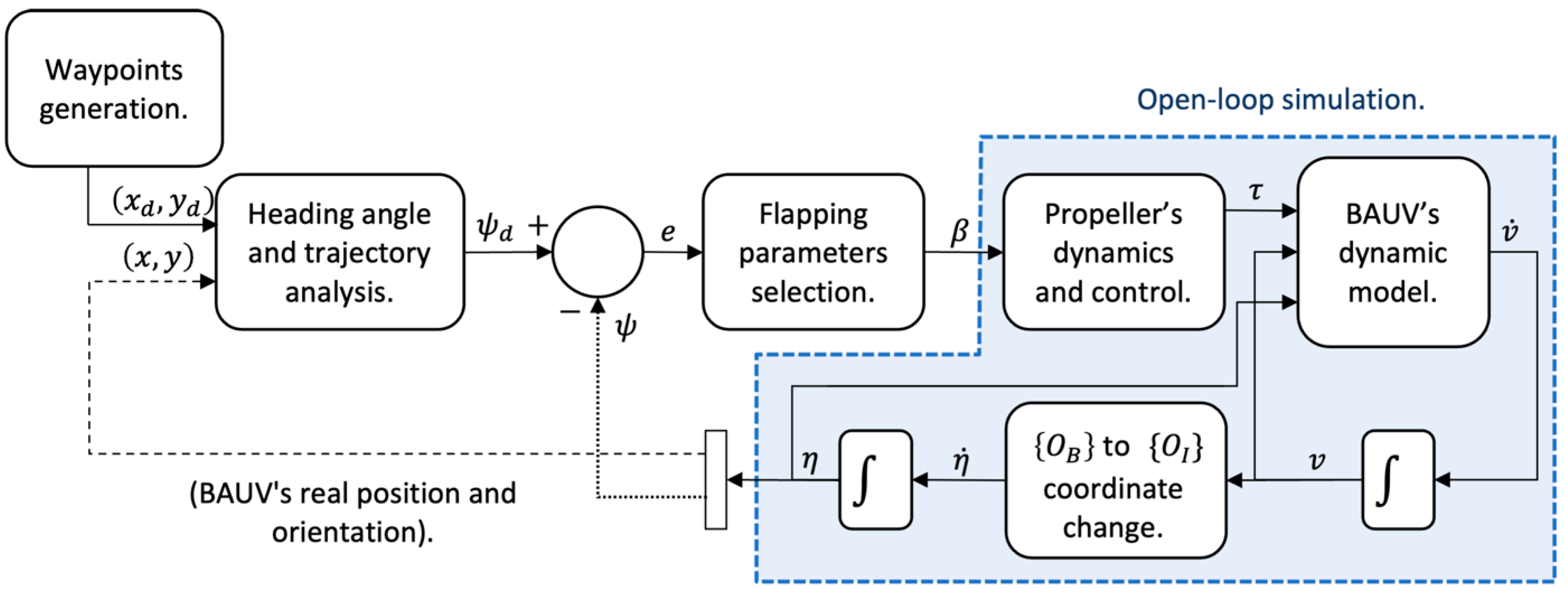
9]. Hence, to correctly implement guidance strategies in the path tracking task of these vehicles, it is necessary to understand how all these factors will affect performance. A proper derivation of the kinematics and dynamic modeling of the vehicle, a force and moment analysis of the propulsion system, and open-loop validations are required to identify which strategies may overcome unwanted reactions.
Several studies have focused on the derivation of the kinematics and dynamic models of biomimetic underwater vehicles. These studies are conducted to identify which behaviors the vehicle will tend to present while swimming. In [
12], Ravichandran et al. performed numerical simulations based on the dynamic modeling of a REMUS autonomous underwater vehicle to which a caudal fin was fixed as the main propeller. By changing its orientation, the caudal fin was able to reproduce dorsoventral and sideways flapping. However, no information of the mechanical design required for the propulsion system to attain such configurations was presented, and a force and moment analysis was not conducted. They found that based on the swimming fashion, the vehicle would tend to follow a circular path while flapping sideways, and straight lines while flapping dorsoventrally. Szymak [
13] developed a mathematical model for a BAUV and a forces and moments analysis produced by a sideways undulating propeller. In his design, the vehicle’s movable tail was considered for thrust generation and two independent pectoral fins were employed to change the cruising orientation. The vehicle achieved a proper thrust once the tail flapping frequency reached 2 Hz at a total amplitude of 20
. During the open-loop simulations, the trajectories presented circular shapes, and the turning direction could be changed when pectoral fins were activated. Majeed and Ali [
14] detailed a mathematical model of a carangiform BAUV. For the vehicle’s dynamics, hydrodynamic added mass and damping terms were computed by approximating the vehicle’s shape to a prolate ellipsoid. Also, to estimate the thrust exerted by the caudal fin, the authors used Lighthill’s Large Amplitude Elongated Body Theory [
15], and the heave and pitch from the vehicle were assumed to be sinusoid functions. The vehicle presented circular paths during open-loop simulations with a tail-sideways-flapping frequency of 1 Hz at a total amplitude of 42
. The authors also demonstrated that biasing the caudal fin’s flapping amplitude to one side made it possible to change the forward direction of the vehicle.
Guiding a BAUV toward a goal is a high priority task. Therefore, a guidance system is required to process the navigation and trajectory presented by the vehicle. This system considers the BAUV’s velocity and attitude, and information regarding the desired goal. Hence, it defines the correction that must be performed to keep on the correct track. Additionally, a control scheme is used to generate signals on actuators to produce the required correction that will help the vehicle swim toward set points. Based on its biomimetic features, the vehicle’s swimming performance will mainly depend on the motion of the propeller and the ways in which forces and moments are exerted.
In the waypoint tracking strategy, the vehicle should reach a preestablished set of coordinates in space (waypoints). The line of sight (LOS) algorithm is one common guidance strategy, where the underwater vehicle maneuvers itself to correct its direction and arrive at predetermined intermediate targets. This is usually done by using coordinate transformations where the desired and actual position of the vehicle are iteratively compared to reduce the error distance, and to compute the desired orientation [
16]. Then, for the complementary control scheme, strategies such as dynamic and robust sliding mode methodologies may be employed to produce desired corrections [
16,
17]. Guo [
18] designed a path tracking controller for a carangiform robotic fish. Inside the control loop, the vehicle’s forward speed and average heading error were fed back to correct the flapping frequency and the bias from the robotic fish tail. By offsetting the tail undulation, turning was achieved and the orientation of the vehicle was iteratively adjusted. Kopman et al. [
19] implemented a waypoint tracking controller based on the heading control of a small two-link robotic fish. The vehicle followed a predetermined path approximated by waypoints positioned close to each other. Some other authors have successfully implemented this strategy by combining control over pectoral fins attached to the vehicle. Wang et al. [
20] controlled the path followed by their robotic ray by producing forward thrust with a tail fin and correcting its direction using its two pectoral fins, accounting for the vehicle’s speed, depth, and course control.
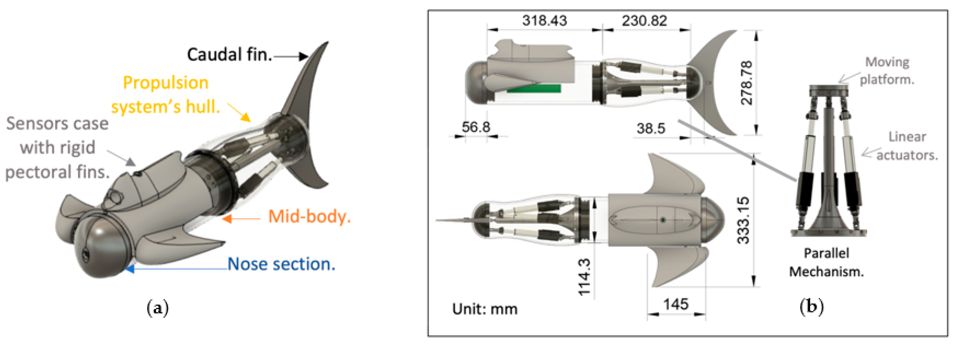
In the present research, a waypoint guidance system for a BAUV is developed and simulated. The BAUV presents a vectored thruster with a novel propulsion system designed by Aparicio et al. [
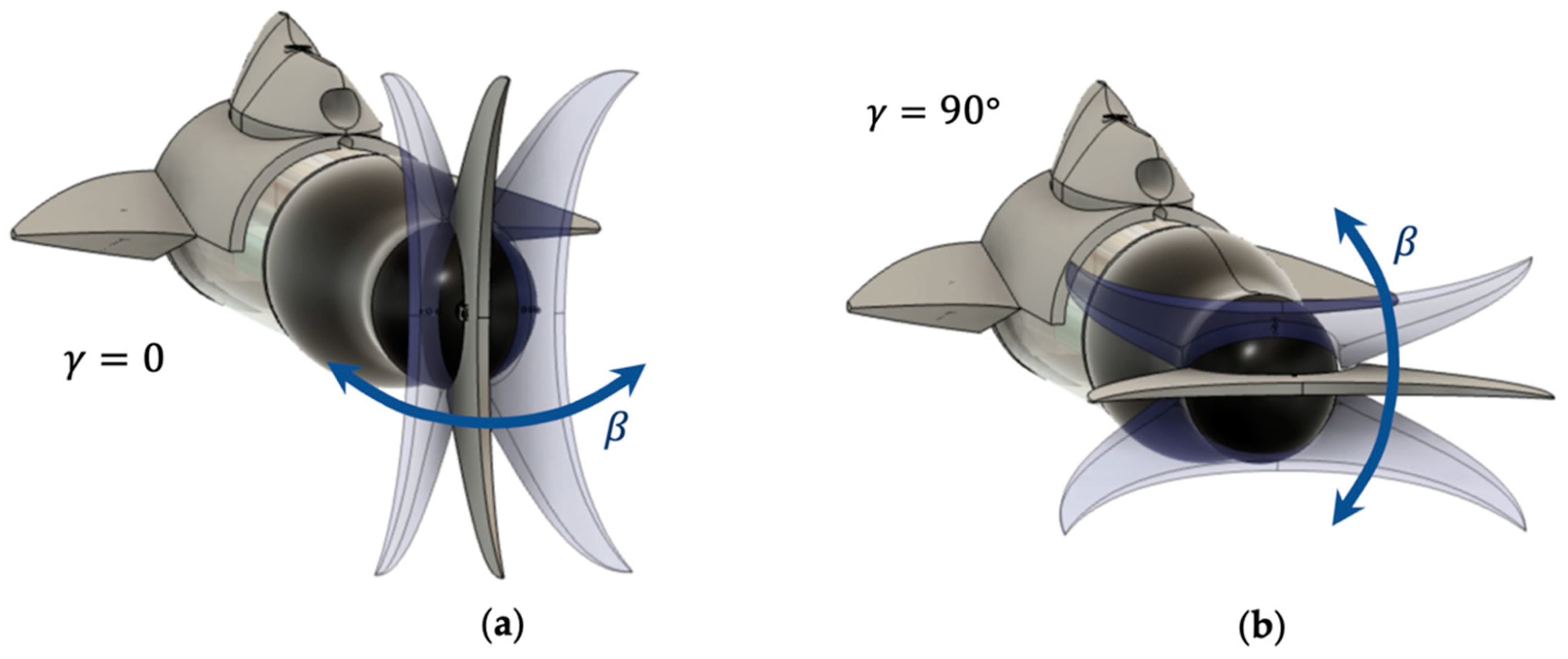
21]. The vehicle follows thunniform locomotion and is driven by a caudal fin. The tail’s flapping frequency, amplitude and offset are regulated by a three-degrees-of-freedom parallel mechanism [
22]. This novel propulsion system allows the caudal fin to change its orientation via sideways and dorsoventral flapping configurations. Then, by only controlling linear actuators, the tail can oscillate in different dispositions, providing excellent vectored thrust and allowing the BAUV to dive and maneuver while swimming.
The present work develops a method of analysis of force and moment produced by such a propulsion system based on the performance of the designed parallel mechanism and its workspace. Also, the vehicle’s kinematics and dynamic modelling are detailed. Further studies on hydrodynamics based on the hull design of the BAUV are described. Then, by considering such models and the novel feature of switching among swimming modes, the underwater performance of the vehicle is simulated in open-loop trajectories. Finally, based on an analysis of trajectories determined by the vehicle’s biomimetic features, a waypoint guidance strategy is developed. The results from open-loop simulations showed how the vehicle tended to describe defined trajectories according to the swimming style and flapping performance from the fin. However, by maintaining vehicle’s forward speed, and by properly implementing a strategy to correct the fish’s heading angle, the BAUV successfully reached predetermined waypoints on the horizontal plane. Hence, by the adequate definition of flapping parameters such as frequency and bias, thrust and moment are regulated to correct unwanted BAUV behaviors. To the best of the authors’ knowledge, even when parallel mechanisms are incorporated to produce vectored thrust on nonbiomimetic underwater vehicles (with turbine-based-propellers) [
23,
24,
25], their incorporation to change biomimetic features (i.e., swimming mode) on BAUVs has not previously been developed. The means by which this novel feature enhances the cruising trajectories of BAUVs is explained in this paper.
This article is divided as follows:
Section 2 details the methods considered during the development of the research. The BAUV design, and mathematical definitions of its hull, kinematics, dynamics, and hydrodynamics are developed. Further, the waypoint guidance strategy and all considerations for the implementation of simulations are detailed. In
Section 3, the results from numerical simulations are presented. A discussion of the results obtained for thrust and moment generation, open-loop trajectories and the incorporated guidance strategy based on the flapping performance of the propeller is presented. Finally,
Section 4 includes final remarks and the conclusion of this paper, as well as explaining some future work that this investigation may lead to.
3. Results and Discussion
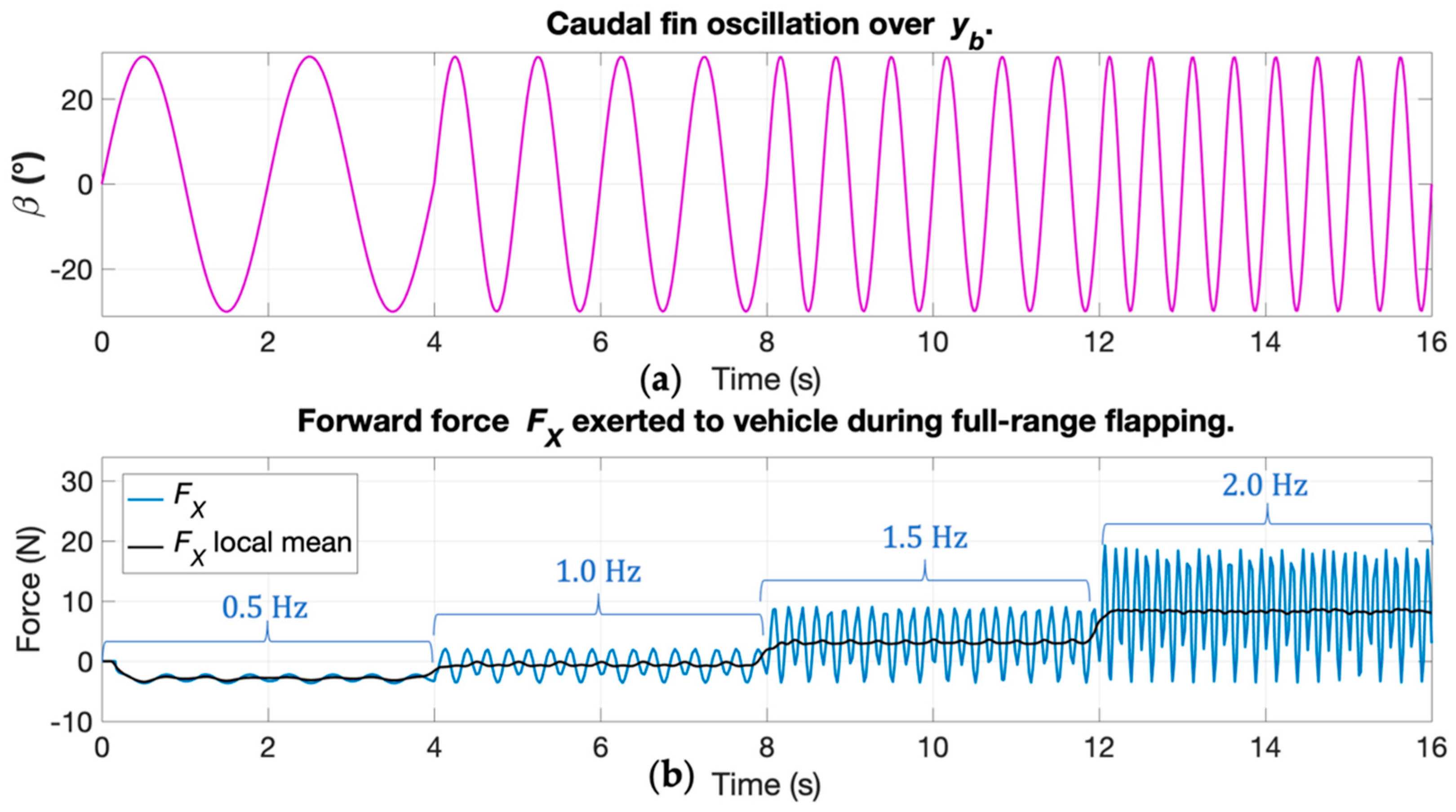
Figure 11 presents graphs of the force produced when the propeller started oscillating. The thrust levels along the vehicle’s centerline
increased once the flapping frequency increased. This means that to push the vehicle and achieve forward momentum, it was necessary to make the caudal fin oscillate more rapidly. During the simulations, the frequency increased by steps of 0.5 Hz every four seconds. As shown in
Figure 11, an estimation of force
was conducted based on the total amplitude oscillation of the caudal fin
, with a flapping frequency ranging from 0.5 to 2 Hz.
Figure 11a describes the caudal fin’s angular position over time, and
Figure 11b shows the force produced from such motion.
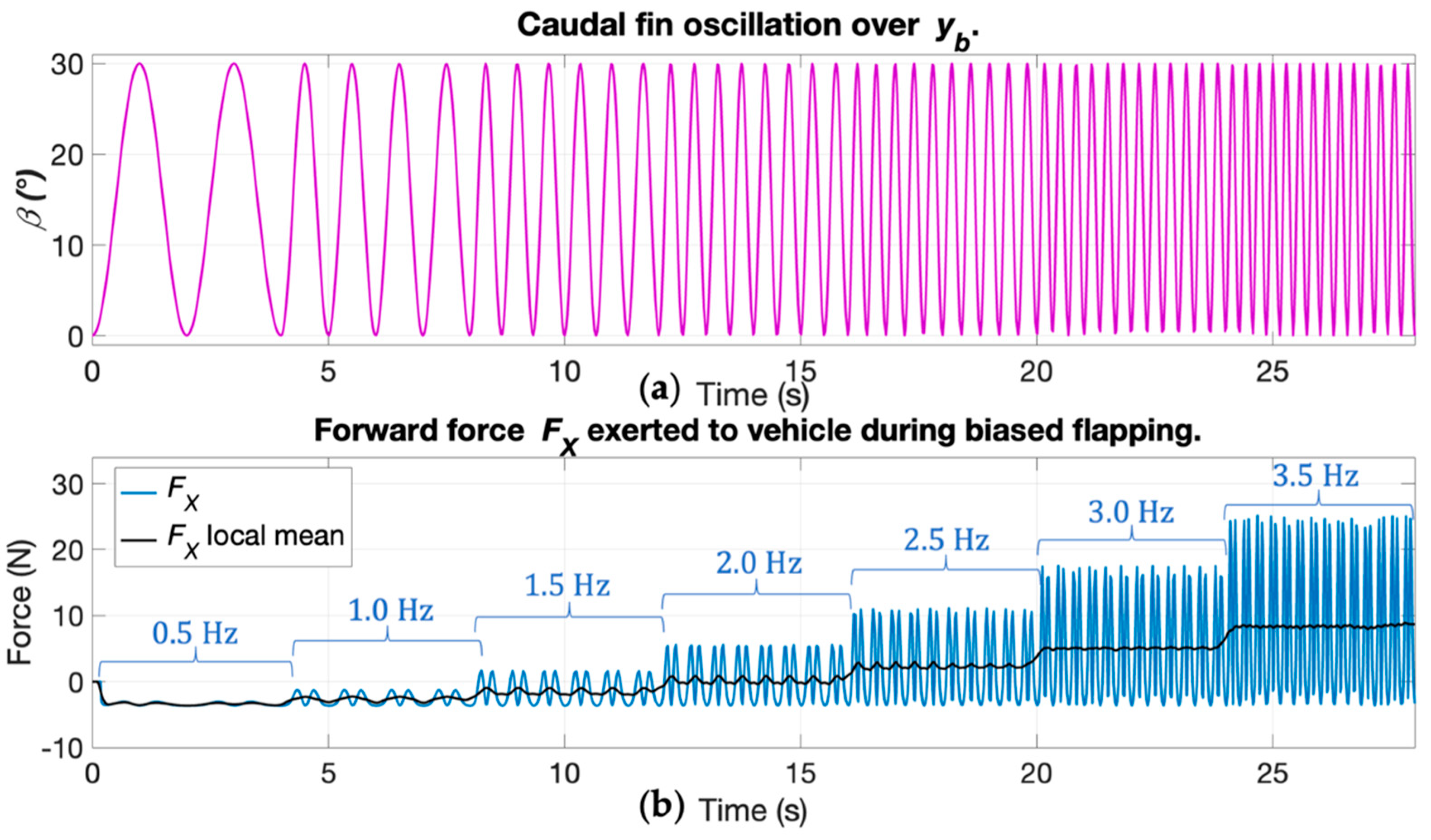
Figure 12 shows the results from the same simulated experiment but only considering biased flapping (i.e., a half fin workspace). Compared to full-range flapping, biased flapping required higher frequencies to push the vehicle forward. Then, based on these results, the propeller was set to flap at 2 Hz when moving at its full range and set to 3.5 Hz when only moving half span.
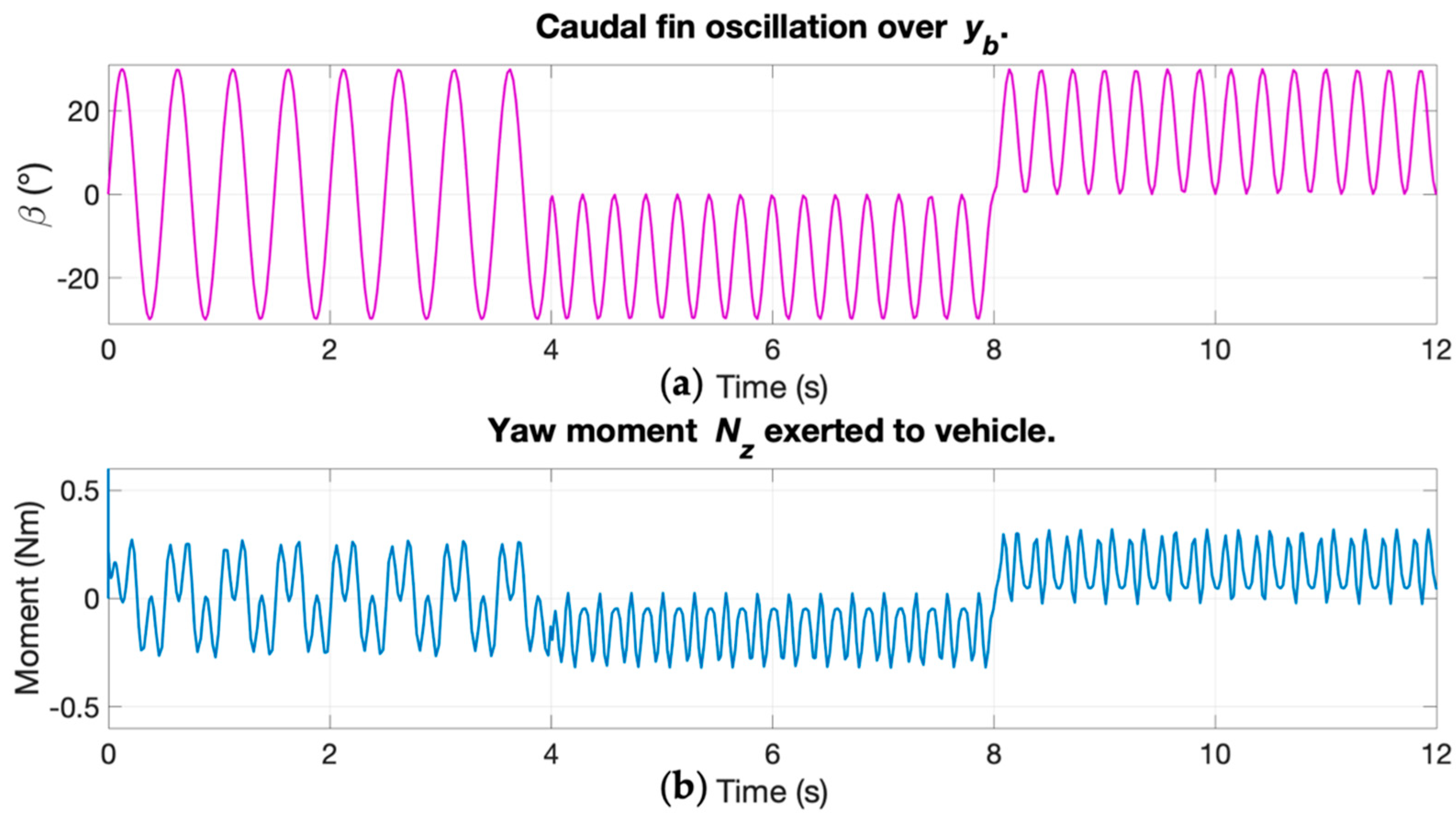
Since the vehicle’s path is controlled based on the correction of its heading angle, the generation of turning moment is of paramount importance.
Figure 13 shows moment
over the
axis based on the flapping performance of the propeller. In
Figure 13a, three different arrangements for flapping disposition are shown. First, the caudal fin followed a full-range trajectory, and was then biased to each side. As determined in the force analysis, the oscillating frequency of the fin was set to 2 and 3.5 Hz for full- and half-range flapping, respectively.
Figure 13b shows how the moment direction changed when biased flapping was induced in the vehicle’s tail. Hence, biasing the caudal fin oscillations changes the vehicle’s orientation, and thus, correction of the BAUV’s heading angle toward desired targets on the horizontal plane may be achieved.
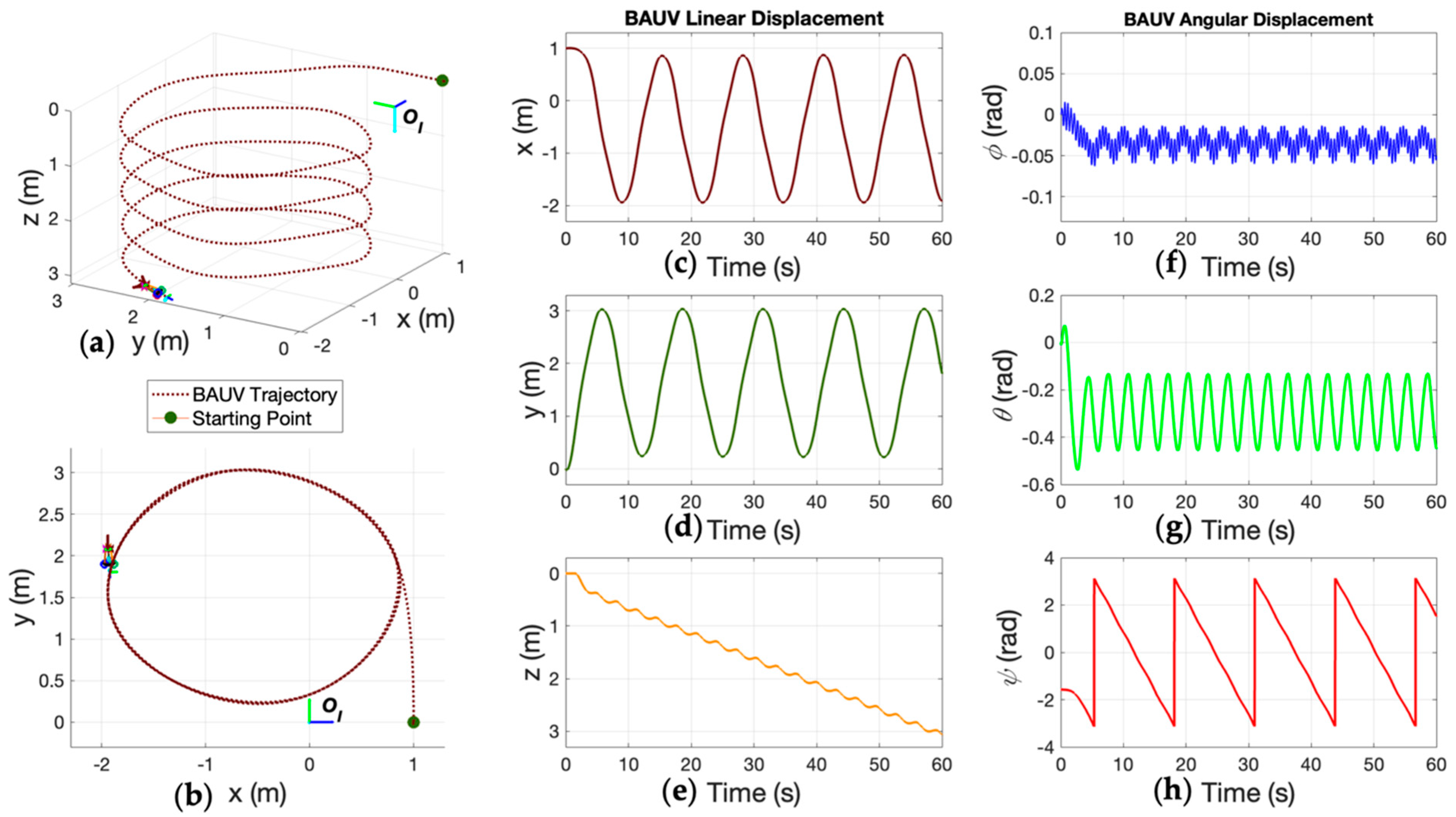
For the second set of simulations,
Figure 14 shows the open loop trajectory of the BAUV when swimming sideways. For this analysis, the propeller was set to flap at full port-starboard range at 2 Hz. The starting position and orientation of the BAUV was set at an arbitrary value, i.e.,
, as established in the examples in
Figure 6. In
Figure 14a, the helicoidal trajectory described by the vehicle is shown from an isometric view, while
Figure 14b presents the top view with a circular path on the horizontal plane. Once the propeller starts oscillating, thrust makes the vehicle move forward and dive. Also, during sideways flapping, a lateral force is produced, coupling force components in the surge and sway directions. This event causes the vehicle to start turning over yaw angle
in the direction of positive surge and sway. Since the propeller kept the same flapping parameters throughout the simulation, the vehicle kept turning, describing a circular path over the
plane. The turning behavior of the BAUV could be corrected by changing the moment produced over the yaw axis to make it rotate in different directions. The linear displacement of the BAUV is shown in
Figure 14c–e, while its angular displacement is shown in
Figure 14f–h.
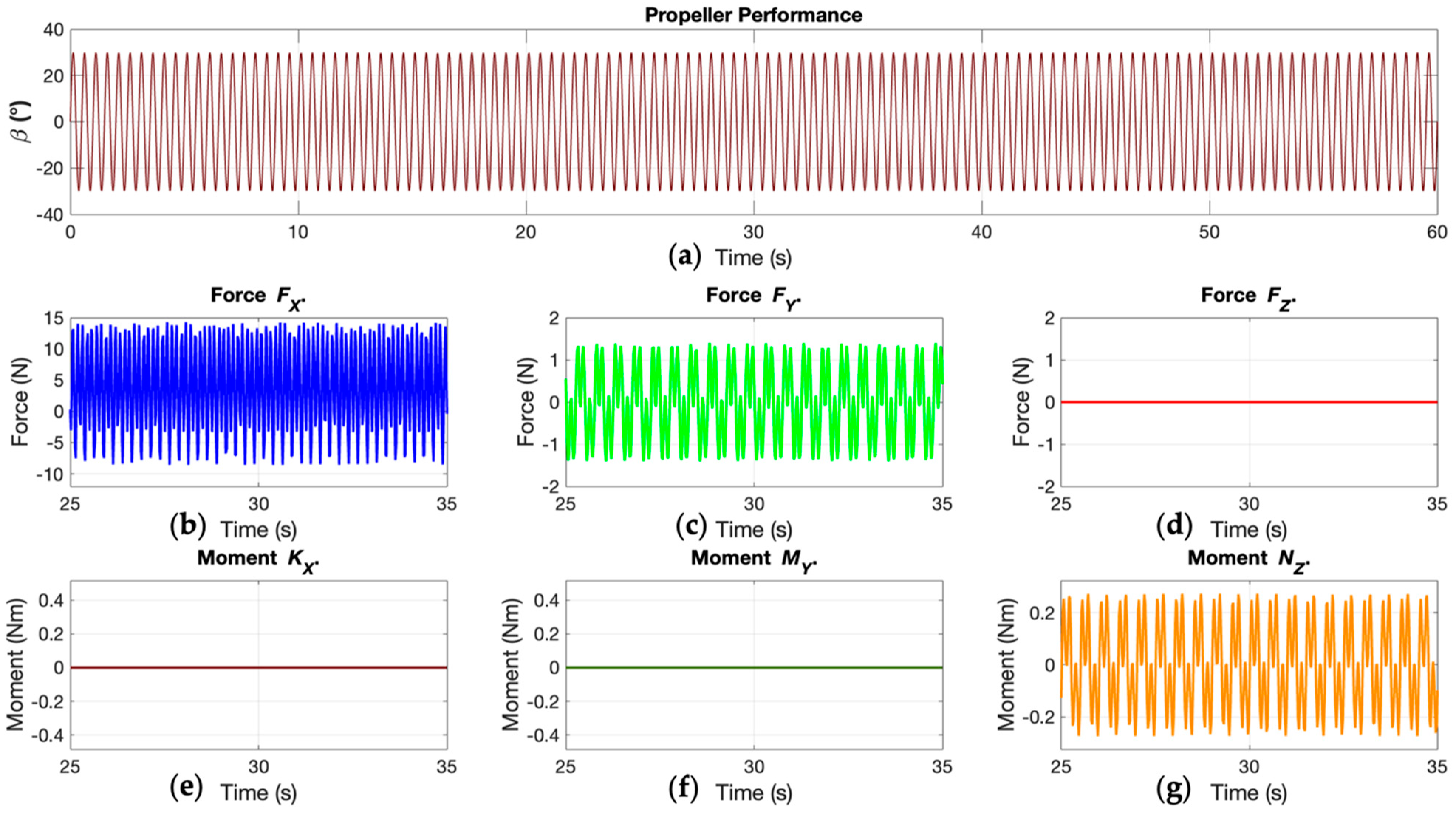
In
Figure 15a, flapping performance
of the fin during the sideways swimming open-loop simulation is described.
Figure 15b–d describe the linear force that was exerted in sideways swimming mode. In
Figure 15e–g, the rotational moment over
exerted by fin’s motion is shown. The thrust and moment exerted by the propeller presented consistent behavior throughout the whole simulation. To avoid the loss of detail in graphs of forces and moments, only a 10 s span is shown. During sideways flapping, linear forces
and
couple, causing motion in directions
and
. Also, this swimming mode tends to produce moment
over
. Then, based on the way in which thrust and moment were produced by the designed propulsion system during sideways flapping, enhanced steering maneuvers over the
plane could be achieved.
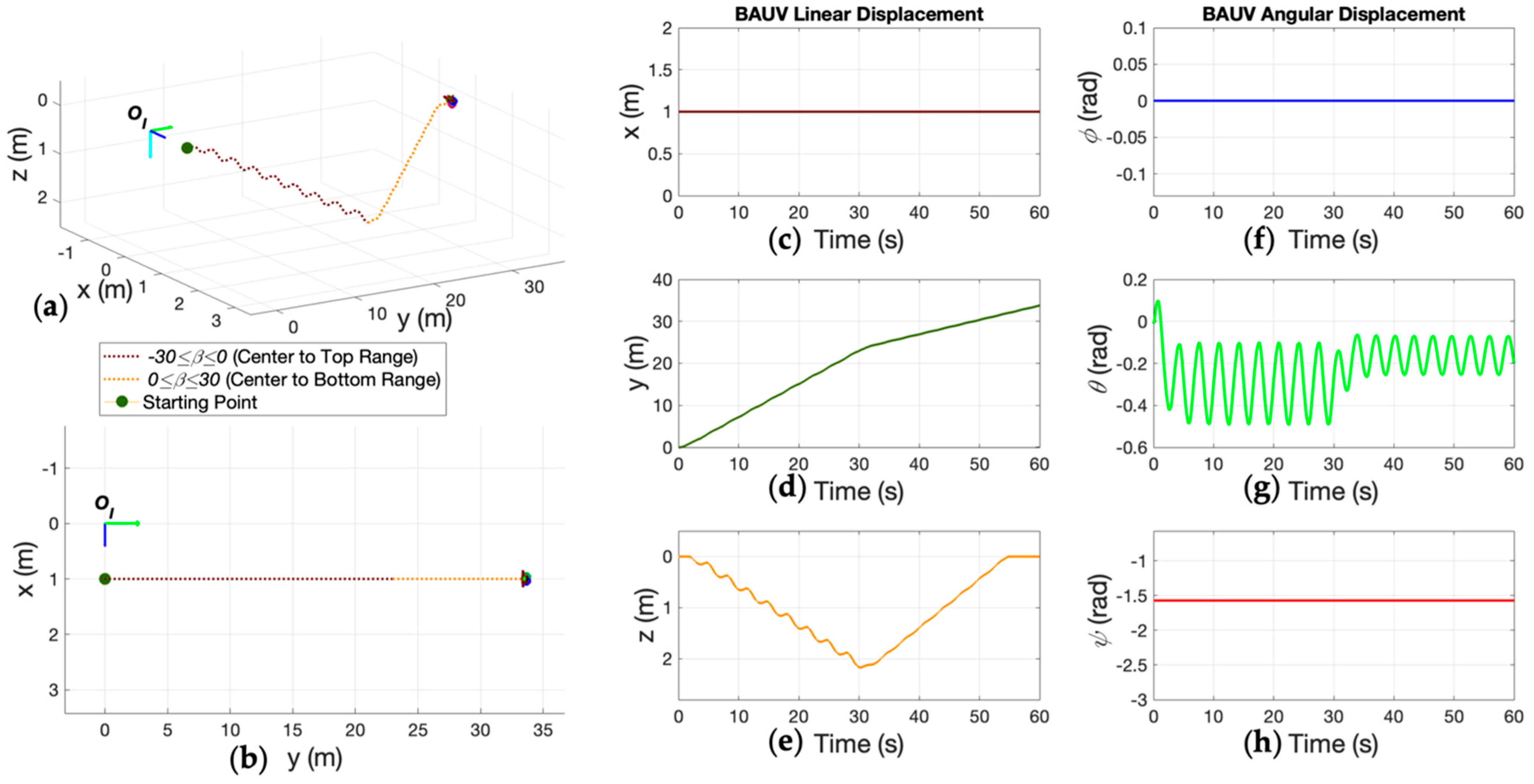
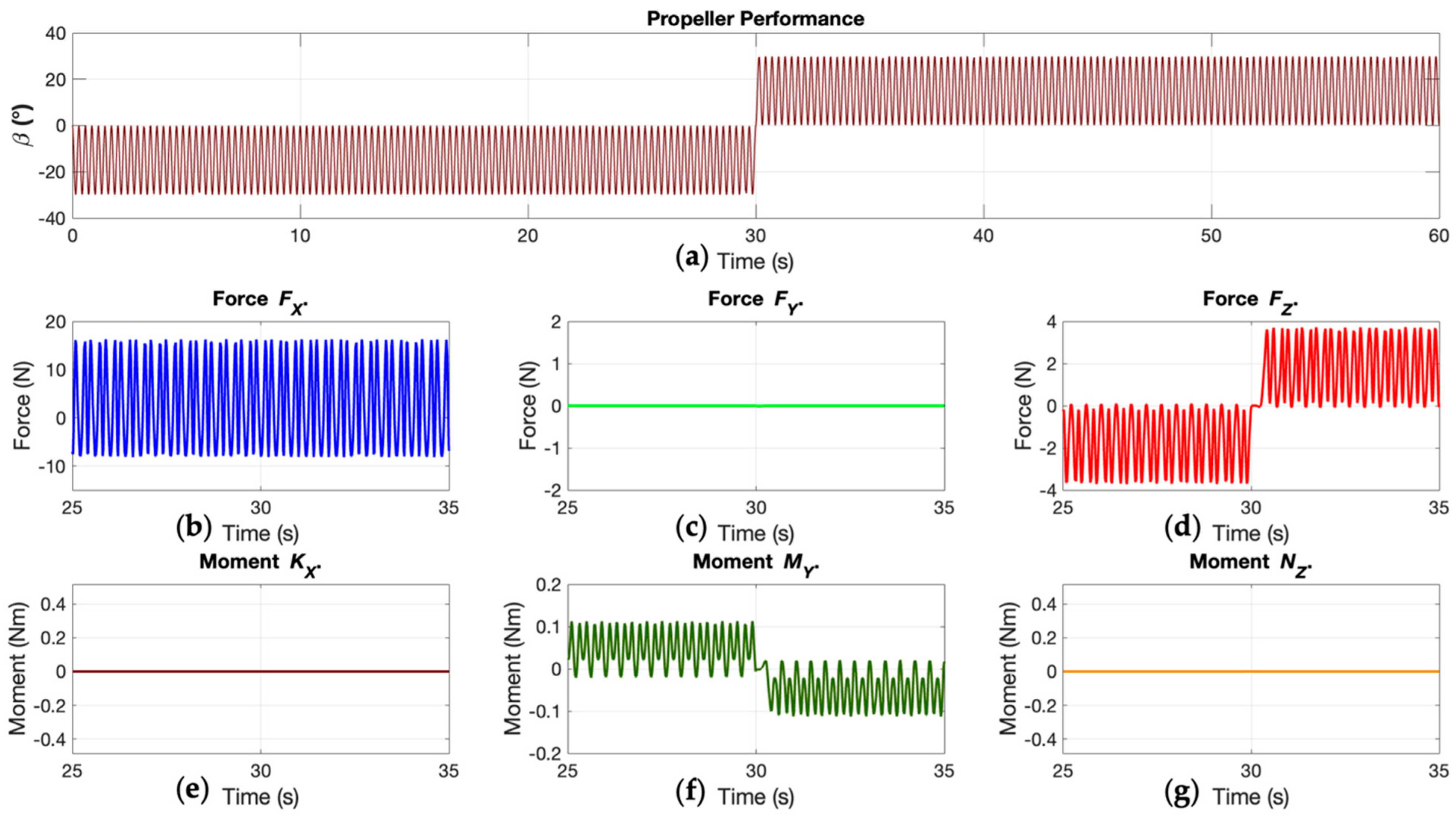
Figure 16 shows the results of setting the BAUV on an open loop mission while swimming dorsoventrally. For a 60 s simulation, the propeller was set to flap at
during the first 30 s, and then at
. This allowed us to change thrust direction in order to visualize how the vehicle reacted. When setting the BAUV to swim dorsoventrally, the vehicle also achieved forward thrust, and better control over diving was obtained when compared to sideways flapping (
Figure 16a).
Figure 16b shows that by applying this swimming method, the BAUV tends to describe straight trajectories. Moreover, the vehicle started diving when the propeller was set to move on the upper side of its workspace (center to top). While diving, buoyant forces acting on the vehicle affected its motion, driving it back over the
axis, as seen on
Figure 16e. When the flapping direction changed to lower-side workspace (center to bottom) of the fin, the thrust exerted on the vehicle allowed it to reach the surface sooner. Also, the BAUV’s linear and angular displacements (
Figure 16c–h) presented more stability than those obtained during lateral swimming. This was because of the up-and-downward motion of the caudal fin during dorsoventral flapping, where lateral forces produced over the vehicle’s body were diminished, and vertical forces could be properly directed.
Figure 17a describes the flapping behavior of the propeller during the dorsoventral swimming simulation. This time, the caudal fin was biased to each side.
Figure 17b–d shows the linear force that was exerted by the fin’s motion with both configurations. Forward thrust
was not affected once the flapping direction changed. However, dorsoventral flapping exerted forces along the
axis. According to the biased flapping produced (center to top/center to bottom),
forces could be properly directed. This caused the vehicle to achieve motion along surge and heave. Finally, dorsoventral swimming mode tended to produce moment over the vehicle’s
axis.
Figure 17e–g shows the moment computed in the simulation.
As seen in
Figure 14 and
Figure 16, a BAUV with thunniform motion will be capable of producing thrust efficiently, thereby attaining excellent forward speed. Nonetheless, a lack of efficient maneuvering will occur when turning and diving. Since the caudal fin’s motion is the only parameter responsible for changing moment and force directions, the vehicle takes longer to react. Furthermore, since changing between flapping modes while swimming is not an energy-efficient strategy, the designed propulsion system only follows one swimming style while performing a task. Then, if the mission comprises following straight trajectories while gaining depth, the best swimming option will be the dorsoventral. Otherwise, sideways swimming would be the best option.
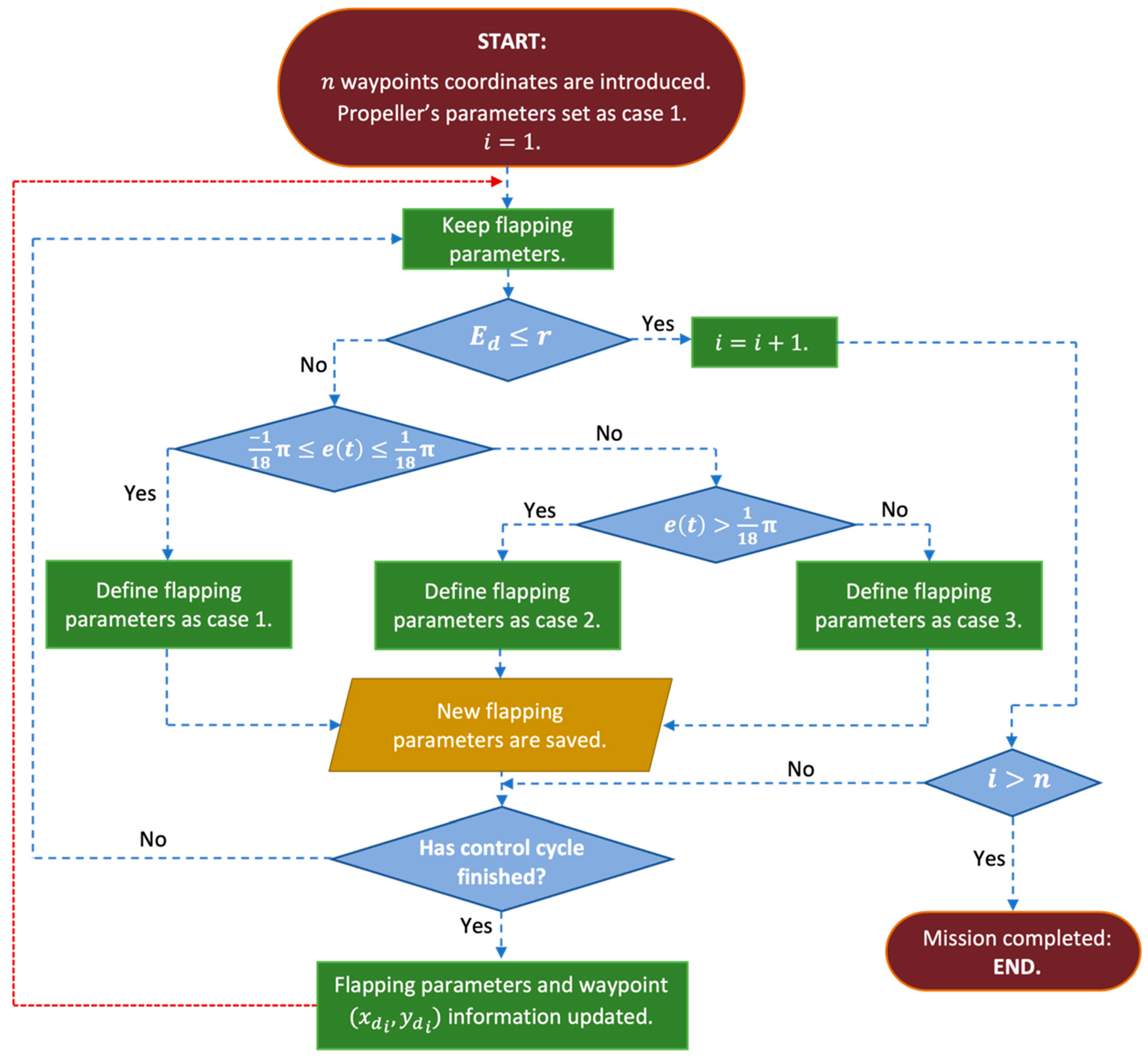
To overcome the low degree of maneuverability of the BAUV, a strategy to regulate the flapping performance of the vehicle’s tail should be developed. Since the vehicle moves forward thanks to the thrust produced by its caudal fin, correcting the direction of such motion becomes a control task. Then, if the flapping performance of the propeller is correctly updated, unwanted behavior may be reduced.
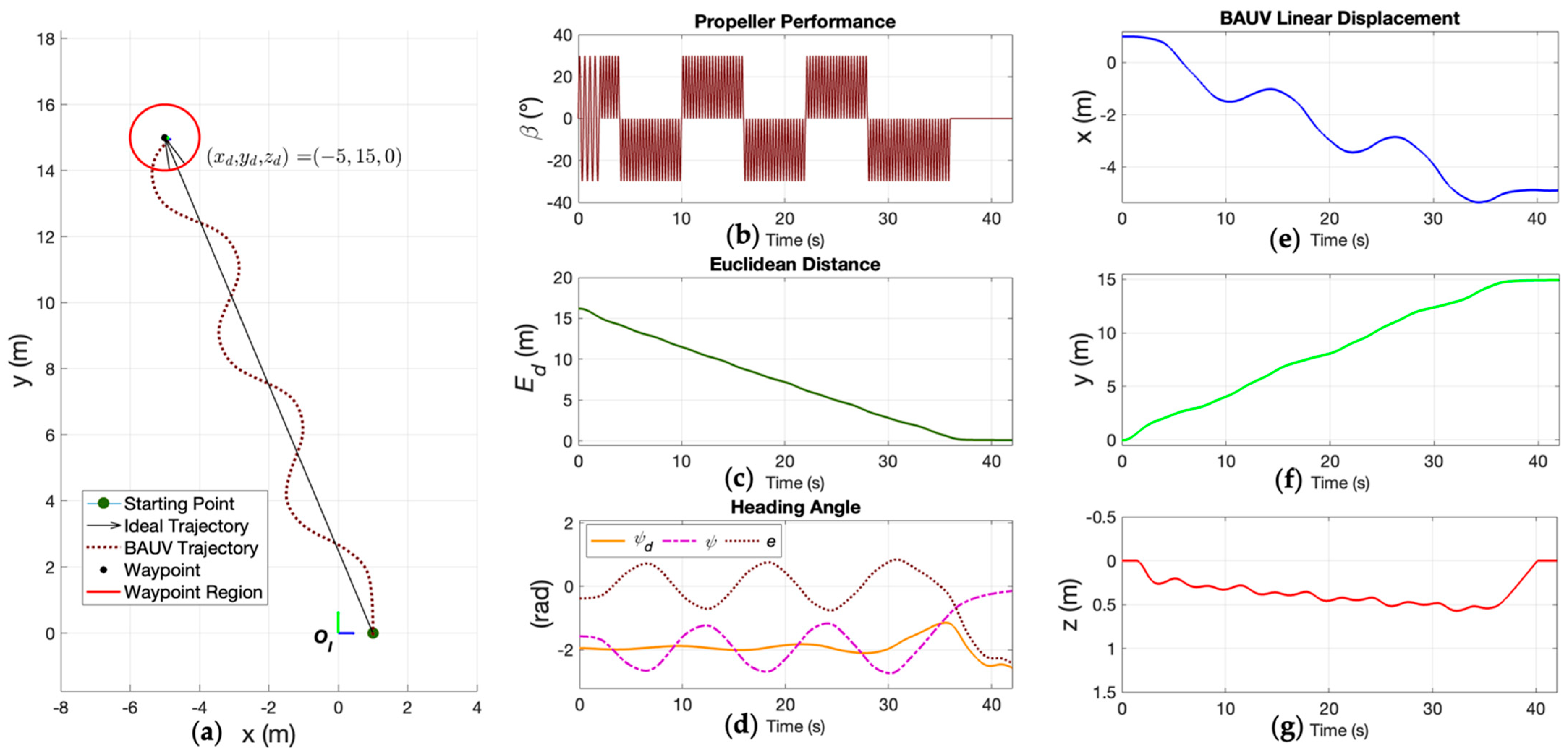
Figure 18 shows the results obtained from the waypoint guidance strategy in the third set of simulations.
Figure 18a illustrates how the BAUV was able to correct its erratic behavior over the horizontal plane while performing sideways swimming. The heading angle correction was achieved by biasing the flapping motion from the caudal fin, as shown in
Figure 18b. Then, by maintaining forward speed and properly updating the flapping parameters after each control cycle, it was possible to correct the orientation of the vehicle relative to the desired goal. In
Figure 18d, tracking errors between
and
are plotted. The Euclidean distance was iteratively reduced (
Figure 18c), and once the vehicle reached the waypoint area, the propeller was turned off.
Figure 18e–g shows the linear coordinates of the BAUV throughout the mission. Once the propeller was shut down, the BAUV floated back to surface (as seen in
Figure 18g).
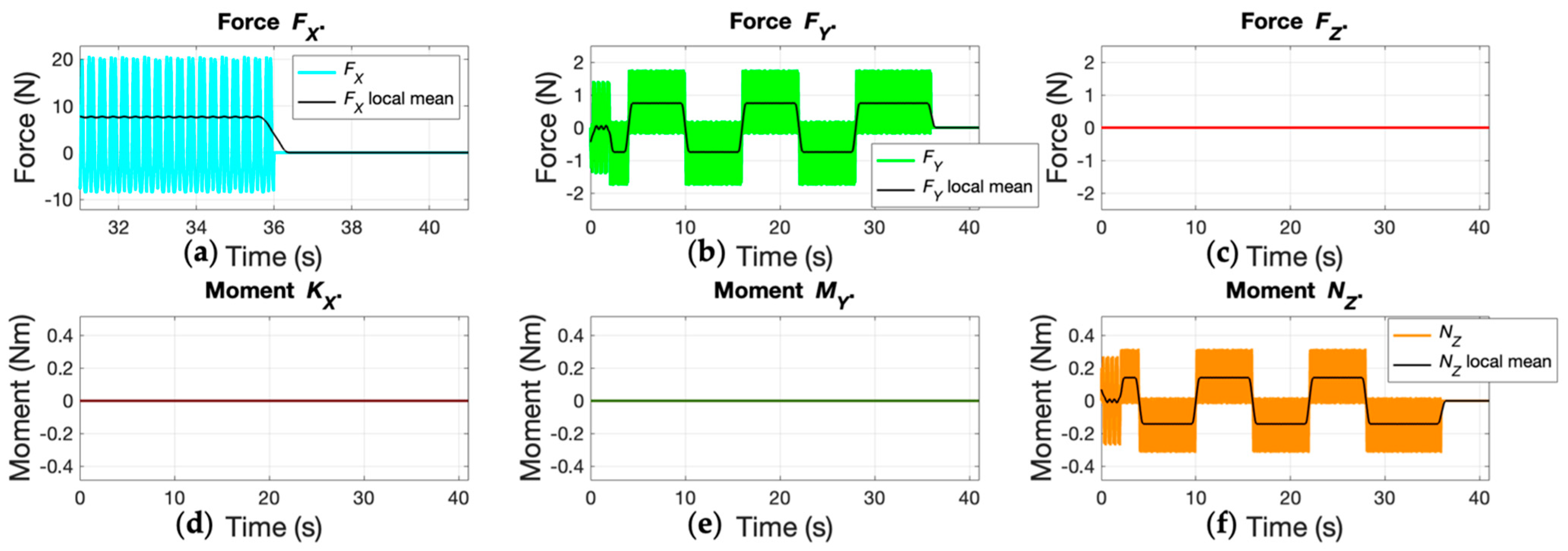
Figure 19 shows the ways in which forces and moments changed during the simulated trial described in
Figure 18. The caudal fin was able to produce a constant forward thrust,
, throughout the mission.
Figure 19a shows how thrust decayed to zero once the propeller was shut down at 36 s.
Figure 19b,f shows the changing behavior of
and
over time.
Table 4 states the accuracy and efficiency obtained from the waypoint guidance strategy applied in this scenario.
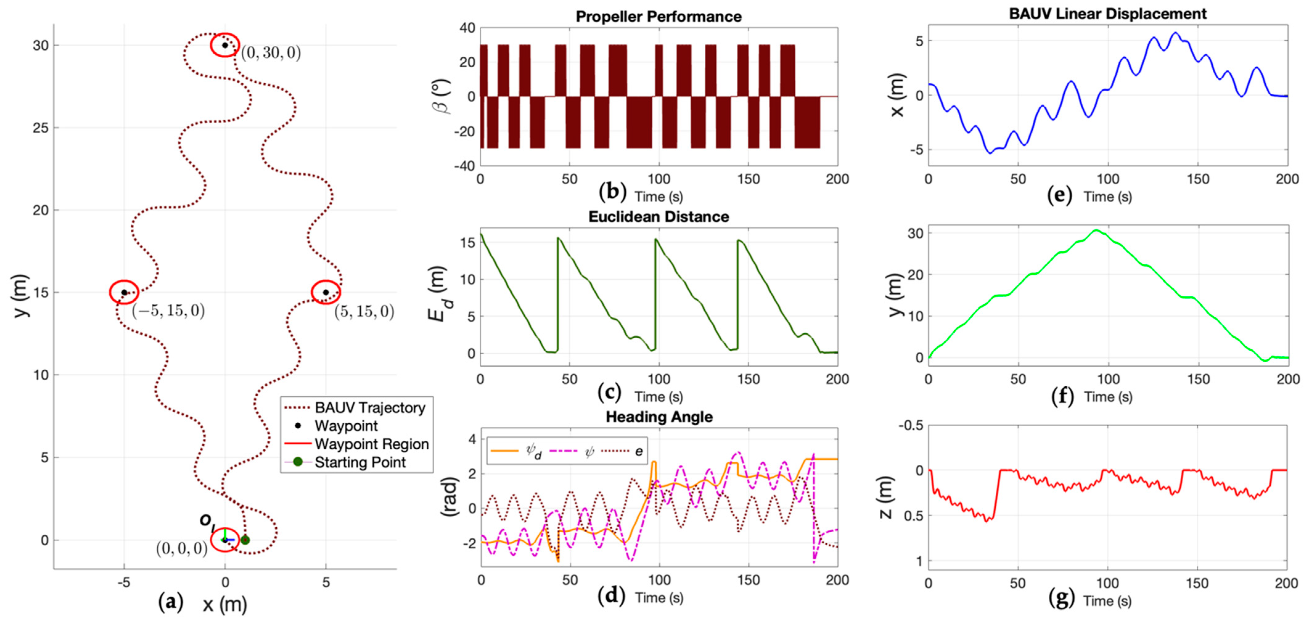
Finally,
Figure 20a shows the BAUV performance when several waypoints were introduced into the guidance system. The vehicle corrected its course (
Figure 20d) toward each of the established targets, ultimately reaching waypoint regions with a proximity
of less than 0.2
(
Figure 20c). Based on these results, the vehicle demonstrated its ability to reach different positions on the horizontal plane; however, its accuracy and performance were limited by its thunniform locomotion. Nonetheless, the proposed propulsion system can overcome such limitations. By using a parallel mechanism, the vehicle’s tail flapping may achieve different speeds and present different behaviors (
Figure 20b). This design for motion generation provides efficient and well-directed thrust. For maneuvering, having a system that can expeditiously bias the propeller is as important as thrust generation. Then, by the development of proper control strategies over the flapping performance of the robotic fish tail, the BAUV will achieve the desired outcomes.
Figure 20e–g shows the vehicle’s behavior while en route to the desired coordinates. In
Table 5, the accuracy and efficiency of the designed strategy based on the distance traveled by the BAUV toward each waypoint are detailed.
As seen in Set 3 of the simulated scenarios, the designed strategy did not consider either the vehicle’s orientation upon arrival or the reduction of the path-tracking error when compared to straight-line trajectories. Some novel controllers may be able to reduce the path-tracking error by controlling the production of forces and moments from the vehicle’s propeller. This might be achieved by the incorporation of robust controllers such as dynamic sliding mode methods or adaptive and/or intelligent controllers. However, in this case, thrust and moment exertion depends on the vehicle’s biomimetic features, which are the result of the proposed propulsion system. In other words, the vehicle’s thrust and maneuvering capabilities are limited by the flapping performance of its caudal fin and the way in which it is driven by the designed parallel mechanism. Even if a control strategy could properly define the required flapping frequency, amplitude, and bias to reduce path-tracking error, the navigation task will depend exclusively on the ability of the propulsion system to produce such movement at the desired moments. From the final simulated scenario, the BAUV showed an average travel-efficiency of about 85% in its navigation toward several waypoints. Also, the average accuracy when arriving at targets was 0.1327 m. These results were achieved thanks to the flapping parameters which were applied to the guidance system, and the control which was applied to the parallel robotic system inside the propeller.
4. Conclusions
In this article, a method for the mathematical modeling of a 6 DOF BAUV with thunniform locomotion was developed. The kinematics and dynamics of the robotic fish and its inner components were studied to comprehend how moments and forces were produced to move the vehicle. For the trajectory analysis, the vehicle’s hydrodynamics were determined. Further, a waypoint guidance strategy based on the flapping performance of the BAUV’s caudal fin was implemented. The vehicle was able to advance and maneuver thanks to its propulsion system, which was responsible for driving the vehicle’s tail at different flapping frequencies and with different dispositions.
The use of a parallel mechanism inside the propulsion system allowed the vehicle’s caudal fin to oscillate at different frequencies and in different ways. Due to this novel feature, the thunniform locomotion of the designed vehicle was enhanced, due to its ability to switch between two swimming modes, i.e., lateral and dorsoventral. From the obtained results, it was seen that the swimming mode directly impacted the vehicle’s performance and its trajectory. While sideways flapping allowed motion on the horizontal plane, dorsoventral flapping presented the advantage of producing stable motion along the vertical plane. Depth and planar motions were achieved by selecting the appropriate swimming mode. Hence, the BAUV’s motion was determined by controlling its tail, since this was the only parameter responsible for generating thrust and moment. Finally, based on the limitations of this locomotion, strategies were developed to correct the course of the vehicle according to the desired goals. With proper control over the flapping frequency and bias of the fin, the designed BAUV achieved forward thrust and moment, allowing it to orient itself relative to several established targets. The waypoint guidance strategy was found to be the optimal means by which to overcome the unwanted performance characteristics that the vehicle tended to present.
In future work, a faster, more robust, and adaptive smart controller for BAUV path tracking needs to be incorporated. More complex techniques such as deep learning and/or neuro-fuzzy algorithms may enhance the process of selecting the flapping parameters. Improved control over parameters such as frequency, bias and amplitude will reduce cruising cost during missions, thereby improving travel efficiency. Hence, complementary controllers to enhance the performance of the parallel mechanism inside the propulsion system should be analyzed. The presence of external disturbances based on different aquatic ecosystems should be incorporated in future analyses to define the expected performance of the proposed design. Further, future work should focus on path planning strategies to allow the vehicle to not only reach preestablished goals, but to properly define which trajectories are the most convenient in the search of such targets.


 ,
, 


