
A Novel MOGNDO Algorithm for Security-Constrained Optimal Power Flow Problems
by
 , , , and
Sundaram B. Pandya
1,
James Visumathi
2,
Miroslav Mahdal
3,*,
Tapan K. Mahanta
4 and
Pradeep Jangir
5 1
Department of Electrical Engineering, Shri K.J. Polytechnic, Bharuch 392 001, India
2
Department of Computer Science and Engineering, Vel Tech Rangarajan Dr Sangunthala R&D Institute of Science and Technology, Chennai 600 062, India
3
Department of Control Systems and Instrumentation, Faculty of Mechanical Engineering, VSB-Technical University of Ostrava, 17. Listopadu 2172/15, 708 00 Ostrava, Czech Republic
4
School of Mechanical Engineering, Vellore Institute of Technology, Chennai 600 127, India
5
Rajasthan Rajya Vidyut Prasaran Nigam, Losal, Sikar 332 025, India
*
Author to whom correspondence should be addressed.
Electronics 2022, 11(22), 3825; https://doi.org/10.3390/electronics11223825
Submission received: 26 September 2022
/
Revised: 15 November 2022
/
Accepted: 16 November 2022
/
Published: 21 November 2022
Abstract
:The current research investigates a new and unique Multi-Objective Generalized Normal Distribution Optimization (MOGNDO) algorithm for solving large-scale Optimal Power Flow (OPF) problems of complex power systems, including renewable energy sources and Flexible AC Transmission Systems (FACTS). A recently reported single-objective generalized normal distribution optimization algorithm is transformed into the MOGNDO algorithm using the nondominated sorting and crowding distancing mechanisms. The OPF problem gets even more challenging when sources of renewable energy are integrated into the grid system, which are unreliable and fluctuating. FACTS devices are also being used more frequently in contemporary power networks to assist in reducing network demand and congestion. In this study, a stochastic wind power source was used with different FACTS devices, including a static VAR compensator, a thyristor- driven series compensator, and a thyristor—driven phase shifter, together with an IEEE-30 bus system. Positions and ratings of the FACTS devices can be intended to reduce the system’s overall fuel cost. Weibull probability density curves were used to highlight the stochastic character of the wind energy source. The best compromise solutions were obtained using a fuzzy decision-making approach. The results obtained on a modified IEEE-30 bus system were compared with other well-known optimization algorithms, and the obtained results proved that MOGNDO has improved convergence, diversity, and spread behavior across PFs.
1. Introduction
Constraint-based optimization problems with multiple objectives are the most prevalent type. In contrast to single-objective optimization problems, multi-objective optimization problems have a wide variety of optimal solutions. The PF is an assortment of perfect responses [1,2]. A multi-objective optimization approach must be able to locate solutions that are uniform in the generated PFs and are workable optimum solutions to address multi-objective problems [3]. Multi-objective optimization approaches are challenged by the simultaneous achievement of these many objectives [4]. MH algorithms are typically tested on simpler, well-known optimization scenarios. However, unlike classic search problems, engineering design tasks can have different specifications. Modifying and developing the algorithm for them is the most effective way to optimize for them. The realm of application of multi-objective optimization algorithms is quite vast, ranging from machining processes [5,6], to vehicle routing [7], to optimizing AI systems [8].
Power systems researchers have been seeking solutions to the OPF challenges for many decades. One issue with managing power systems and making plans for modern electrical energy networks is working with systems that use non-conventional sources of energy. Ullah et al. [9] developed a hybrid phasor particle swarm optimization and gravitational search algorithm to address the OPF problem in the wind and solar energy systems that are connected to electrical power grids, while accounting for the control variables (PPSOGSA). For the OPF problem with wind and solar systems, the developed PPSOGSA algorithm produced outstanding and helpful results. In Elattar’s research, the OPF problem was principally modelled mathematically using a combined heat and power system with stochastic wind energy. On an IEEE 30-bus test system under various test situations, the suggested method was assessed. The formulation of the OPF problem covering energy sources and the suggested approach to solve it produced effective answers in contrast to pre-existing algorithms [10] that were used to address similar problems. Anongpun et al. [11] used IEEE 30- and 118-bus test systems to study the use of enhanced particle swarm optimization (PSO) to solve a multi-objective OPF problem using a wind energy system that combined chaotic mutation and stochastic weights. When compared to the other algorithms included in their study, the suggested method produced better results. Salkuti [12] used the glowworm swarm optimization method to offer a solution to a multi-objective OPF problem requiring a modern electrical energy system that utilized wind energy. On IEEE 30- and 300-bus test systems, the methodology was examined in many operational scenarios. The simulation findings indicated that the proposed methodology might offer an alternative. A flower pollination algorithm was used by Kathiravan et al. [13] to address the OPF problem using coal-based, wind, and solar energy systems. In a variety of test situations, the authors used their method to test systems for the IEEE 30-bus and Indian utility 30-bus. Duman et al. [14] used differential evolutionary particle swarm optimization to address the OPF problem (DEEPSO) with manageable wind and solar (PV) energy sources. IEEE 30-, 57-, and 118-bus test systems were used to evaluate the DEEPSO technique to explore the issue under various objective functions. DEEPSO produced better simulation results when compared to the other optimization approaches that were looked at [14]. They recommended using FACTS devices such as a thyristor-controlled phase shifter (TCPS) and a thyristor-controlled series capacitor (TCSC) to solve the OPF problem. To account for the uncertainties associated with wind energy installation, they used chaotic maps and a modified version of the PSOGSA (particle swarm optimization and gravitational search algorithm). The method presented [15] appears to be a potential approach for a solution based on the findings of simulations. Biswas et al. [16] solved the OPF challenge, which incorporated coal-based, wind, solar, and small-hydro energy sources coupled to IEEE 30-bus test systems, by running multiple rounds of the multi-objective evolutionary algorithm. The constrained multi-objective population extremal optimization (CMOPEO) technique was used to handle the wind and solar-integrated OPF problem by Chen et al. [17], who also tested the method on an IEEE 30-bus for different scenarios. Additionally, research has been done on the evolutionary particle swarm optimization (EPSO) [18], the hybrid differential evolution and symbiotic organisms search algorithm (HMICA-SQP) [19], the success-history-based adaptation of differential evolution with superiority of feasible solutions (SHADE-SF) [20], and the hybrid modified imperialist competitive algorithm and sequential quadratic programming algorithm (HMICA-SQP) [21]. Pandya and Jariwala [22] addressed single and multi-objective OPF issues by integrating with various sustainable energy sources using recently developed metaheuristics algorithms. Biswas et al. [23] analyzed the integration of three FACTS devices, wind turbines, and coal-fired power plants. The success history-based adaptive differential evolution (SHADE) method was used to conduct the investigation. According to the “No Free Lunch (NFL)” theorem [24], no metaheuristic can solve every issue that occurs in real-world situations. This theorem has opened the door to the creation of both novel metaheuristic techniques and improvements to existing ones.
When using the Generalized Normal Distribution Optimization method [25] in multi-objective optimization scenarios, several things need to be taken into account. The initial problem in multi-objective generalized normal distribution optimization is balancing convergence and divergence archives. The algorithm’s generated solution set is filtered according to a certain quality metric, and the non-dominating solution set is kept in separate, external archives. In the literature, there are numerous recommendations for constructing archives that could be employed in the multi-objective Generalized Normal Distribution Optimization method. The pre-defined maximum size archives are widely employed, since more non-dominating solutions can emerge quickly. The algorithm’s ability to begin with the straightforward determination of the required population size and the terminal condition is the most noticeable feature of the GNDO. The location of the person is automatically changed by the generalized normal distribution function (GNDO), which has a simple construction. The benefits and drawbacks of the GNDO algorithm are as follows:
- It offers a faster and smoother convergence, especially for difficult problems, and it strikes the perfect balance between exploration and exploitation.
- Local minima are less likely to become entangled in relaxed convergence.
- Effortlessly simple, adaptable, and simple to use
- The traditional GNDO may have issues with convergence trends or become stuck in narrow, deceptive optima for challenging optimization tasks, such as high-dimensional and multimodal problems.
Currently, both conventional and non-conventional energy sources require more studies. The current body of research recommends using coal-based plus wind and FACTS devices, combined with single and multi-objective optimum power flow (MOOPF) problems. The conventional IEEE 30-bus network has been altered to include non-conventional sources for research purposes. Using Weibull PDF, non-conventional units’ stochastic behaviors are calculated. The generating cost is suitably adjusted to account for reserve cost if these stochastic units are over-estimated and adjusted for penalty cost in the case that they are underestimated. Using the Generalized Normal Distribution Optimization method, Pareto solution clusters are discovered for the multi-objective problem. The following is a list of the contributions made by this study:
- This work focuses on the mathematical modelling of the single and multiple-objective OPF issue modelled, which takes into account both conventional units and non-conventional sources of energy units, as well as FACTS devices.
- The appropriate probability density functions (PDFs) are modeled in the second stage to describe the wind power plants’ random behavior.
- Stochastic non-conventional sources of energy sources are among the single and multiple-objective OPF issues for which the Non-Dominated Sorting Generalized Normal Distribution Optimization (NSGNDO) technique is used to develop solutions.
- Studies and performance evaluations of the MOGNDO algorithm using empirical comparisons are conducted.
The notion of the mathematical models for coal-based power, wind power, and FACTS devices is presented in Section 2 of the study. An explanation of the objectives that need to be optimized is included in Section 3. Section 4 provides an explanation and illustrations of the multi-objective GNDO technique. Section 5 presents numerical results and discussion, and Section 6 provides concluding remarks.
2. Mathematical Representations
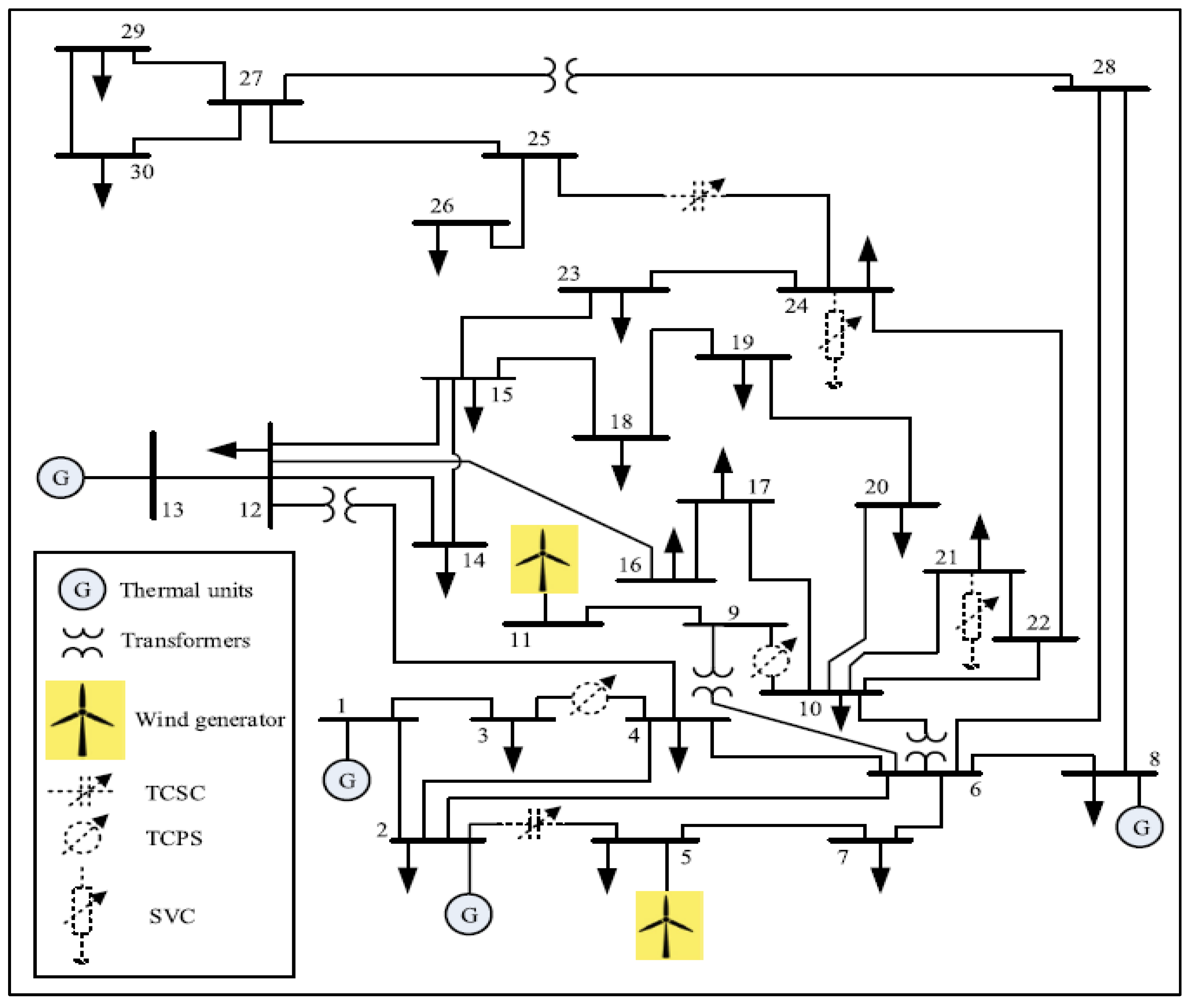
The case studies presented here restructure the original IEEE 30-bus test apparatus. The modified approach incorporates wind turbines and FACTS devices, and is listed in Table 1. The equipment used for the analysis is depicted in Figure 1. The placement and ratings of FACTS devices are depicted in the diagram with dotted lines because they have been optimized. The section below provides information on the costs of traditional coal-based production facilities and plants using non-conventional sources of energy.
2.1. Cost of Coal-Based Power Units
The generalized quadratic equation for the calculation of generation cost is expressed in (1) in $/h [23]:
For a more practical case, the valve point effect included:
The values of both coal-based price constants and emanation constants with various scenarios are shown in [23].
2.2. Toxic Gas Emanation
Polluted gases are released by using coal-based plants. So, toxic gas emanations in tons per hour can be determined as (in ton/h):
The toxic gas emanation constants of coal-based power plants are taken from [22].
2.3. Direct Cost of Stochastic Non-Conventional Sources Plants
It is particularly challenging to integrate non-conventional energy sources into the power grid since they are stochastic. The independent system operator (ISO) is responsible for managing these non-conventional energy sources. Due to this, the private operator must contract with the grid or ISO for a specific quantity of planned power. The scheduled electricity must be maintained by the ISO scheduled power. If these non-conventional sources are unable to maintain the planned power, the ISO is liable for the absence of power. So, if a need arises, there are spinning reserve requirements. This spinning reserve increases costs for the ISO, and this circumstance is known as an overestimation of non-conventional sources. Conversely, if non-conventional sources formed more energy than was planned, it might go to waste, due to underuse. Therefore, the ISO must accept the penalty charge. The scheduled power cost, the overestimation cost caused by the spinning reserve, and the penalized cost caused by the underestimation are the three costs related to electricity. The direct cost linked to wind farms is demonstrated with the scheduled power from the same sources as:
2.4. Indeterminate Non-Conventional Sources of Wind Power Cost
Due to the erratic nature of wind, the wind farm occasionally produces less energy than expected. This means that if demand increases, it needs the spinning reserve to maintain the agreed-upon amount of scheduled power. It is sometimes feasible that the real power generated by wind farms won’t be enough to meet demand and will have lower values. Such power is referred to as exaggerated power by an ambiguous resource. To control this kind of uncertainty and provide end users with a reliable power source, the network ISO operates spinning reserves. The price of hiring a backup generator to supply the overestimated power is known as the reserve cost.
Reserve cost for the wind unit is formulated by:
The possibility exists that the wind farm will generate more power than is required, which is the opposite of the overestimation scenario. Underestimated power is the term used to describe such a situation. If there is no provision for managing the output power from coal-based units, the excess power will be lost. Regarding the extra power, the ISO needs to be penalized.
The penalty charge for the wind unit is given by:
2.5. Uncertainty Models of Stochastic Wind Units
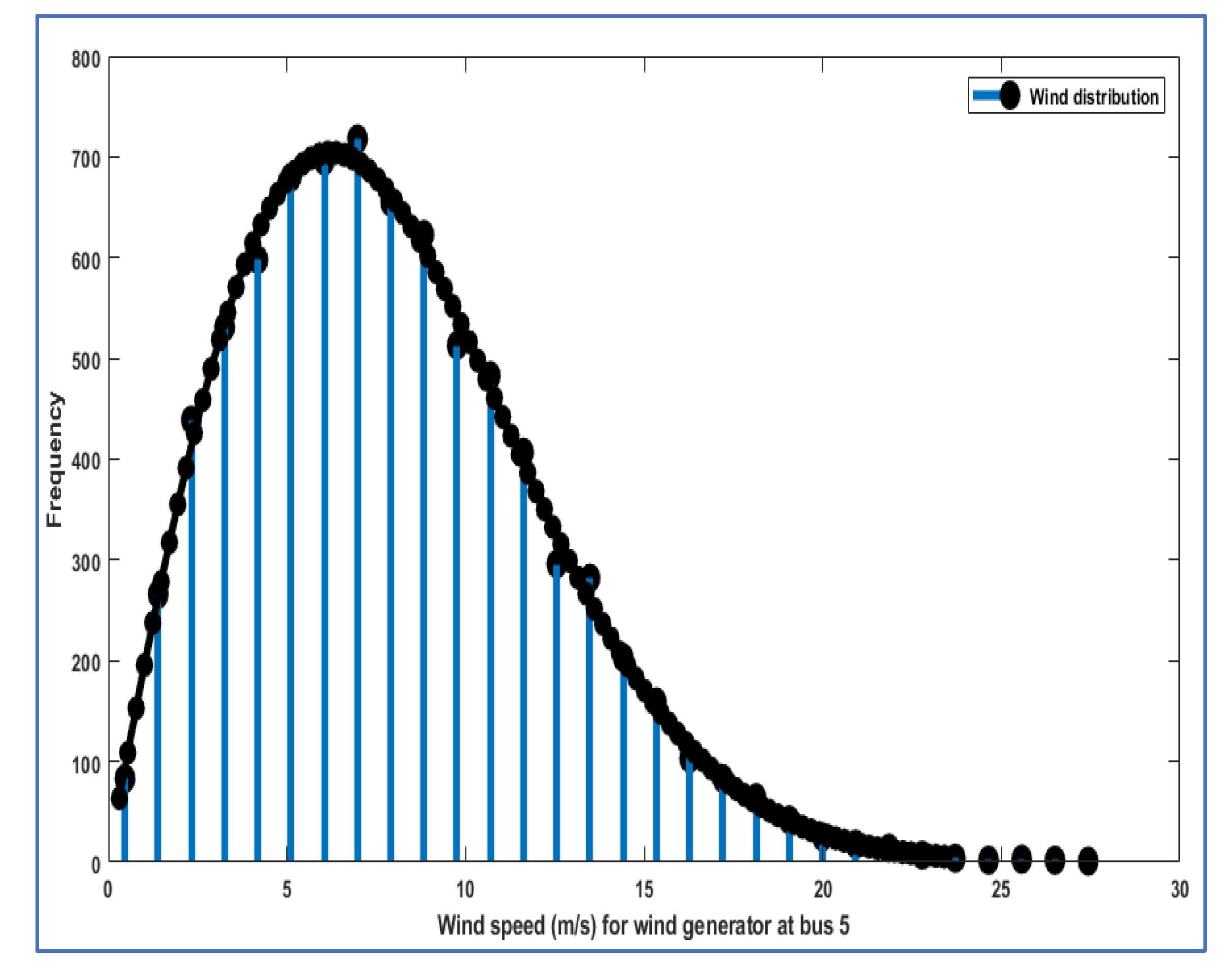
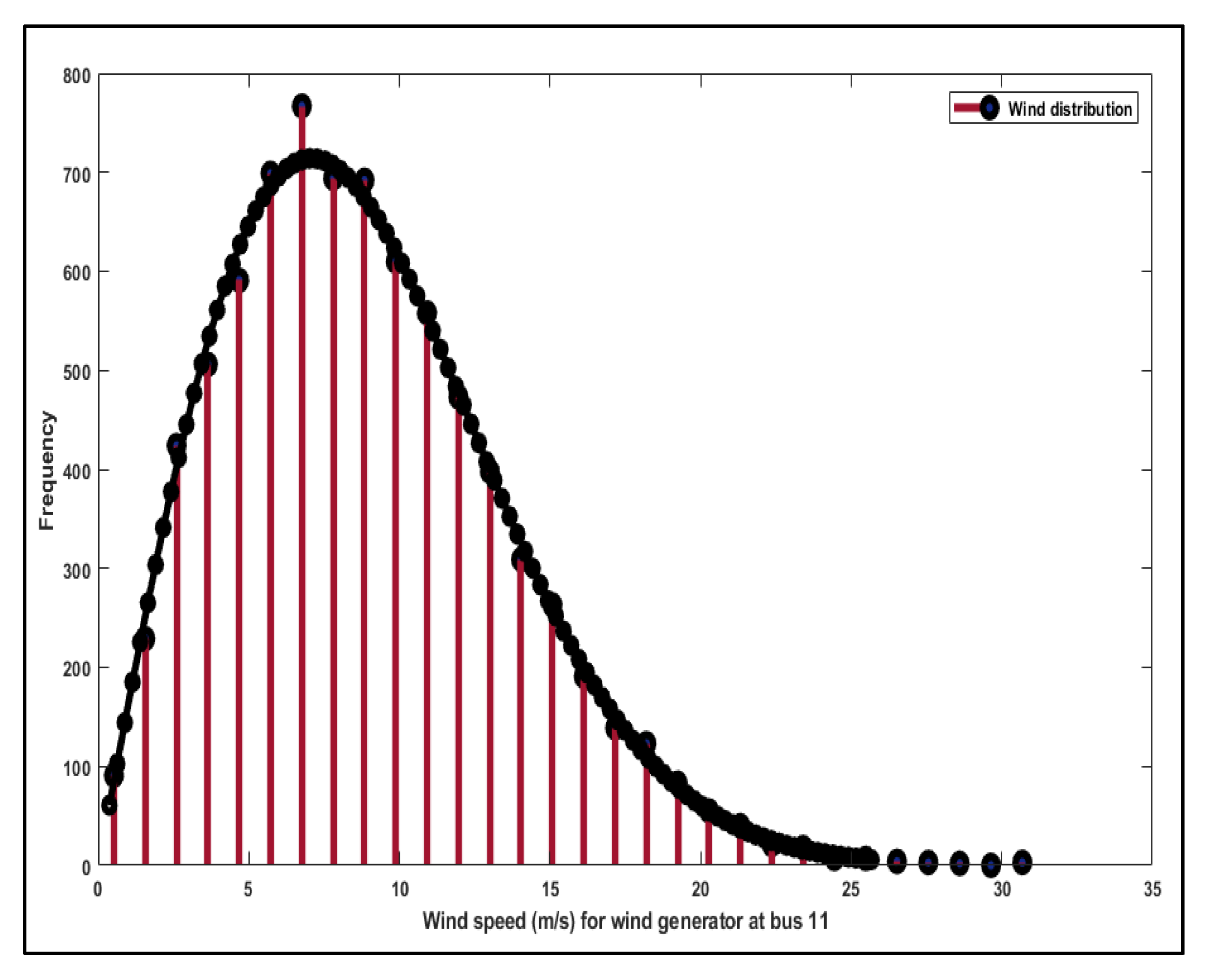
In the redesigned IEEE-30, the wind power generating units installed at buses 5 and 11, which were originally thermal generators, were replaced. It should be noted that, as for a comparison point of view with the published reference article [23], in this paper, the thermal DGs were also replaced with the wind turbines. This will ensure compatibility of the results obtained by the proposed algorithm to the already published research article [23]. The scale (c) and shape (k) constants for the proposed Weibull model are detailed in Table 2.
The Weibull curve and wind frequency distributions in Figure 2 (for the bus 5 wind plant) and Figure 3 (for the bus 11 wind plant) were produced using 8000 Monte-Carlo settings. The standard provided explains the need for wind turbine design and specifies the maximum turbulence class IA that is confirmed to operate at the highest yearly average wind velocity of 10 m/s at hub height. The formed shape and scale ) parameters of wind farms are given particular attention, because their highest Weibull mean value is fixed at around 10. It is commonly known that the wind speed distribution follows the Weibull PDF curve.
The following formula can be used to calculate the probability of wind velocity v, in m/s, pursuing the Weibull PDF with shape factor (k) and scale factor (c) [23]:
The Weibull distribution’s mean is given as follows [23]:
and the gamma function is expressed in Equation (9):
2.6. Average Power Calculation for Wind Plants
The combined outputs of the 25 turbines in the farm are taken as the wind unit connected at bus 5. Every turbine has a 3 MW output rating. The wind velocity affects the wind turbine’s precise output, which varies. We used the following equations to express turbine output power in terms of wind velocity (v) [23]:
The Enercon E82-E4 design specification is referred to for the 3 MW wind turbine. The various speeds are = 3 m/s, = 16 m/s, and = 25 m/s.
2.7. Wind Power Probabilities Calculation
In certain ranges of wind speeds, uncertain wind generation is noticeable. The generated power would be 0 if the wind speed was greater than or less than the cut-out speed or cut-in speed. The turbine thereby produces the specified amount of power within the range of the rated and cut-out wind speeds. These are possible ways to describe the likelihood of these areas [23]:
Between the cut-in velocity and the rated velocity of the wind, the wind production remains constant. The following can be used to express the likelihood of the continuous zone [23]:
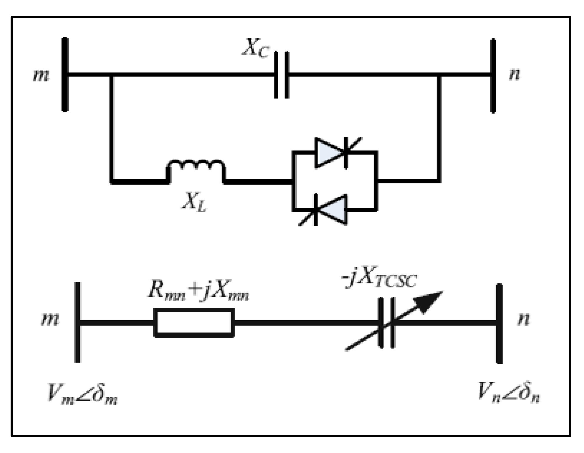
2.8. Thyristor-Controlled Series Compensator (TCSC) Modeling
The basic circuitry of the TCSC is depicted in Figure 4. It consists of a fixed series capacitor (XC) and a reactor (XL) operated by a thyristor. For the TCSC to function as a variable capacitive reactance, reactance is taken into consideration. By varying the firing angle () of the thyristors, the inductive reactance is changed, and for high values of inductive reactance, the least corresponding capacitive reactance is produced (Open circuit Inductive branch). As a result, the TCSC’s effective reactance with constant capacitive reactance and variable inductive reactance can be written as [23]:
2.9. Model of Thyristor-Controlled Phase Shifter (TCPS)
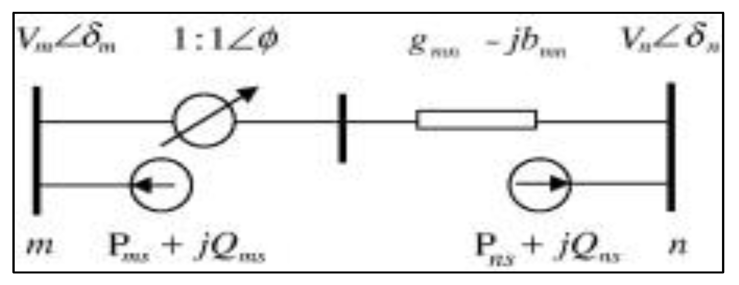
Figure 5 displays the model of the TCPS placed between the line that connects buses and . The power flow equations of the line can be expressed as below, assuming that is the phase shift angle is introduced by the TCPS:
2.10. Model of Static VAR Compensator (SVC)
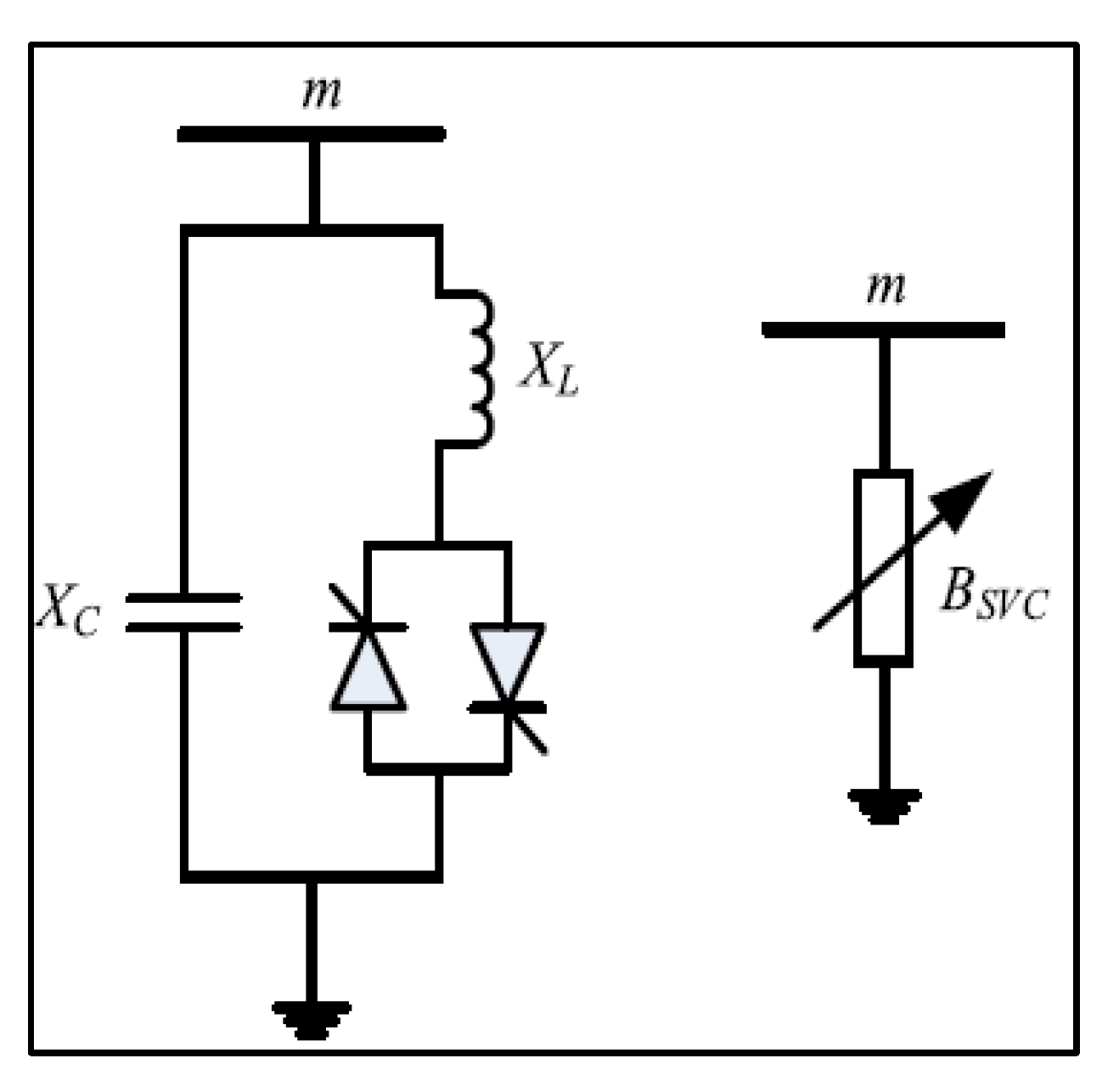
The basic circuit architecture and the SVC model are depicted in Figure 6. It is made up of a thyristor-controlled reactor ( and a fixed capacitor (. By changing the thyristor firing angle , the reactance can be changed. The equivalent susceptibility is computed as:
where
The reactive power offered by the SVC can be expressed in terms within the context of power flow:
3. Objectives of Optimization
The best active power allocation and the best VAR power allocation are goals in the OPF. The following are some examples of how this section incorporates the goals of wind power flow optimization.
3.1. Reducing Overall Costs While Using Non-Conventional Energy Sources
Objective 1:
Minimizing the whole cost is the first goal. Direct, reserve, and penalty charges for non-conventional resources are added to the coal-based unit cost to determine the overall generation cost. Therefore, the comprehensive cost for coal-based and wind power plants is denoted as:
Minimize—
3.2. Reduction of Voltage Variation with the Use of Non-Conventional Energy Sources
One of the most crucial safety and administrative superiority lists is the bus voltage. By restricting the voltage deviations of the PQ bus from 1.0 for each unit, the improving voltage profile will be acquired. The objective function is going to come from:
Objective 2: Minimize—
3.3. Minimization of APL Including Non-Conventional Energy Sources
The optimization of actual power losses (MW) maybe calculated by:
Objective 3: Minimize—
3.4. Enhancement of VSI Including Non-Conventional Energy Sources
The index is the most important indicator for evaluating each bus’s voltage constancy margin, since it keeps the voltage constant within a reasonable range during typical operation. For every PQ bus, the index offers a scalar number. Between ‘0’ (no load) and ‘1’ is where the index is located (voltage collapse). The following formula is used to get the jth bus’s voltage collapse indicator amount:
The objective function of voltage stability enhancement is written by:
3.5. Minimization of Entire Gross Cost Including Non-Conventional Energy Resources
The generating cost is significantly higher in the latter scenario, whereas the loss is greater in the former, as shown by Objectives 1 and 3. The requirement for an aim that includes both the cost and the loss is increased by this very circumstance. Making a cost model that converts the loss into an equivalent energy cost is a straightforward way to take into consideration both goals. The price of energy taken into account in this analysis is $0.10 per kWh. The goal of gross cost in dollars per hour might be stated as follows:
3.6. Equality Constraints
Power flow equations provide equality boundaries, and demonstrate that both real and fictitious power generated in a system should fulfill the load demand and system losses:
3.7. Inequality Constraints
Inequality bounds are the operational boundaries of devices and the security bounds of lines and PQ buses.
- Generator bounds:
- Security bounds:
- FACTS devices bounds:
The real power output limits of coal-based and wind units are shown in Equations (43) and (44), respectively. Then, Equations (45) and (46), which show the VAR power size of producing units, are used. The overall voltage regulator buses are shown in NG. PV bus voltage restrictions are shown in Equation (47), while PQ bus voltage restrictions are shown in Equation (48), where NL is the number of PQ buses. When NL is the total number of lines in a system, Equation (49) can be used to calculate line loading limitations. Equations (50)–(52) show the limits of the TCSC, TCPS, and SVC devices, respectively.
4. Generalized Normal Distribution Optimization Algorithm
4.1. Inspiration
The normal distribution theory serves as the foundation for GNDO. The normal distribution, commonly referred to as the Gaussian distribution, is a crucial tool for describing natural phenomena. The following is a definition of a normal distribution. Assume that random variable follows a probability distribution with location and scale parameters, and that its probability density function may be written as:
Following that, can be referred to as a normal random variable, and this distribution can be referred to as a normal distribution. Two variables, the location parameter and scale parameter, are part of a normal distribution, according to Equation (53). It is possible to describe the mean value and standard deviation of random variables using the location parameter and scale parameter, respectively. In general, population-based optimization approaches’ search procedures consist of the three stages listed below. The scattered distribution contains all initialized people to start. Following that, everyone begins to move in the direction of the global optimal solution, and are guided by the designed exploration and exploitation tactics. The optimal answer is attained, and everyone congregates around it. Multiple normal distributions can adequately characterize this search process. To put it more precisely, individuals’ positions can be thought of as random variables with a normal distribution. The ideal position and the mean position are farther apart in the initial stage. The positions of all people exhibit a significantly high standard deviation. The gap between the average and ideal positions gradually narrows in the second stage. With each individual’s position, the standard variance decreases. The standard deviation of each individual’s location can be as low as possible in the final stage, which also sees the shortest distance between the mean position and the ideal position.
4.2. Local Exploitation
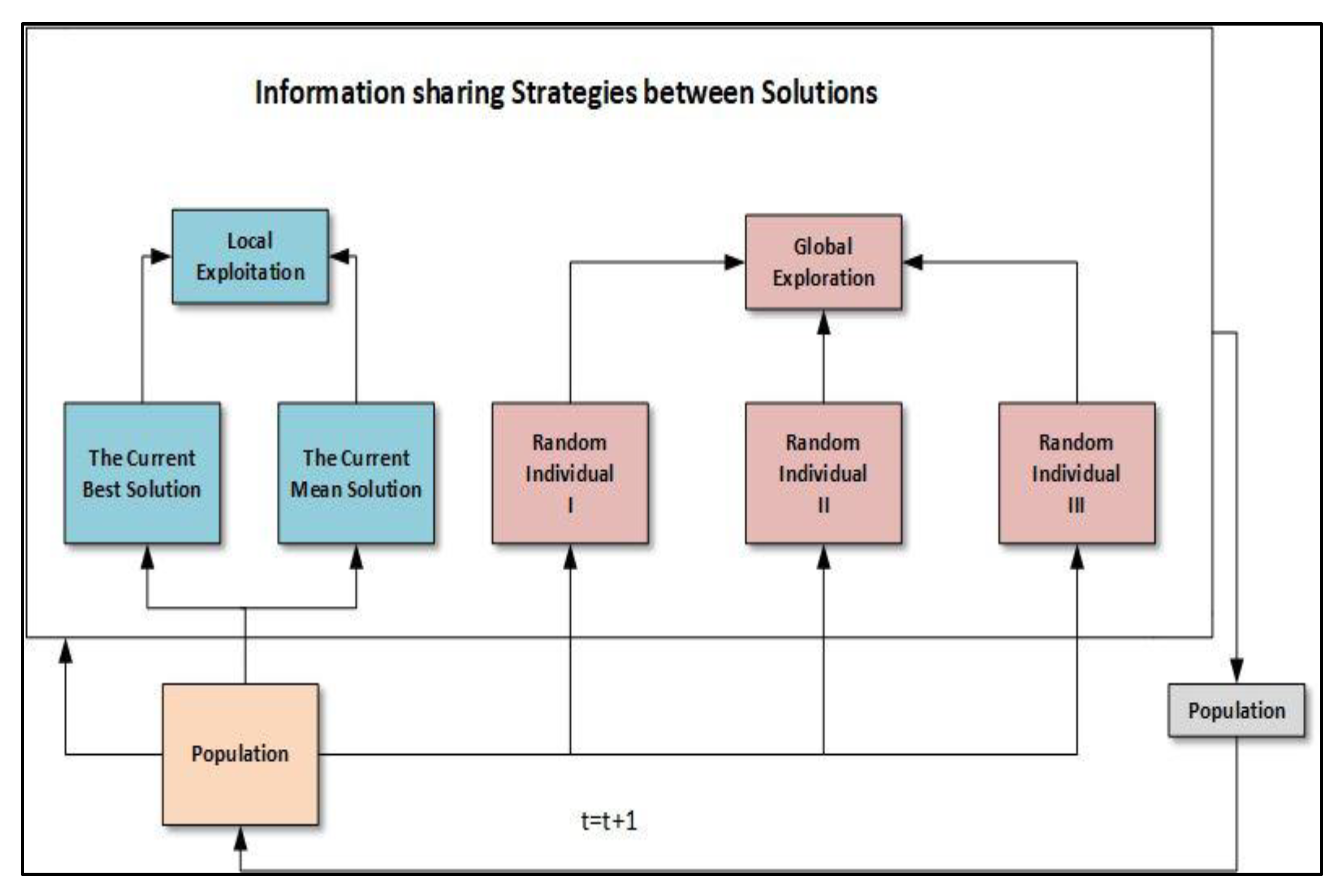
The suggested GNDO framework is depicted in Figure 3. As can be seen, GNDO has a fairly straightforward structure, and its local exploitation and global exploration information exchange mechanisms are built specifically for GNDO. The generalized normal distribution model that has been constructed—which is based on the current mean position and the present optimal position—is the foundation for local exploitation. Three people that were chosen at random were tied to global exploration. The following provides a thorough overview of the two learning strategies. Local exploitation is the process of locating better solutions within a search space made up of everyone’s present placements. A generalized normal distribution model for optimization can be constructed based on the correlation between the population’s distribution of people and the normal distribution:
where is the trailing vector of the ith individual at time , is the generalized mean position of the ith individual, is generalized standard variance, and is the penalty factor. Moreover, ,, and can be defined as
where , b, , and are random numbers between 0 and 1, is the present fitness location, and is the mean location of the present population. In addition, can be calculated by:
4.3. Global Exploration
A speech space is searched globally to identify promising regions. The worldwide exploration of GNDO is based on three individuals who were chosen at random, as shown in Figure 7.
where and are two random numbers subject to the standard normal distribution, is called the adjust limit and is a random number between 0 and 1, and and are two trail vectors. Moreover, and can be calculated by:
where , and are three random integers selected from 1 to N, which meets p1 ≠ p2 ≠ p3 ≠ i. In the context of Equations (60) and (61), the second term to the right of Equation (59) can be referred to as the local learning term, indicating that solution p1 shares information with solution , and the third term to the right of Equation (59) can be referred to as the global information sharing term, indicating that the information is provided to the individual by the individuals p2 and p3. To balance the two information-sharing options, utilizes the adjusted parameter . Furthermore, because and are random numbers with a typical normal distribution, the search space for the GNDO can be expanded when conducting a global search. The absolute symbol in Equation (59) is used to stay steady with the screening mechanism in Equations (60) and (61).
4.4. The Implementation of the Proposed Method for Optimization
This section presents the GNDO implementation. The defined local exploitation and global exploration tactics serve as the foundation for the proposed GNDO. The two tactics are equally important and equally likely to be chosen for the GNDO. Additionally, similar to other population-based optimization methods, GNDO initializes its population by;
where D is the total number of design variables, is the jth design variable’s lower boundary, is its upper boundary, and is a random number between 0 and 1. Note that neither a local exploitation approach nor a global exploration strategy will guarantee that the ith individual will find a better solution. A screening system is created to ensure that the population of the future generation receives the best solution, and it may be described as:
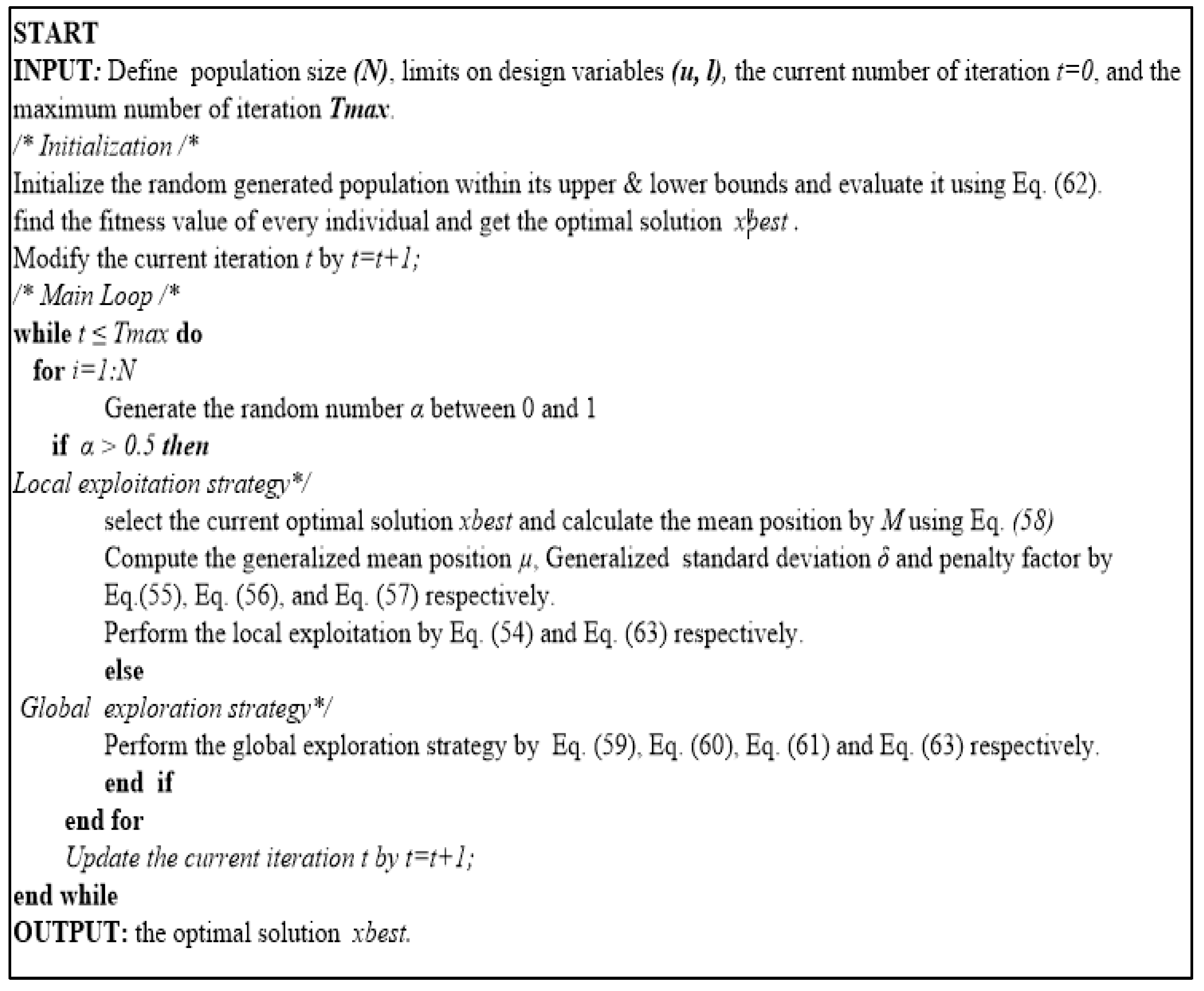
Figure 8 provides the pseudocode of the GNDO.
4.5. Basic Definitions of Multi-Objective Optimization
One optimization technique or tool that allows for more than one objective function to be used for any type of issue is multi-objective optimization. The following is a formulation of the fundamental elements of any multi-objective optimization:
where signifies the ith equality constraint, denotes the ith inequality constraint, n signifies the number of equality constraints, p denotes the number of inequality constraints, denotes the decision/optimization variables, the minor and upper limits of the decision variables are represented by lb and ub, the number of decision variables is denoted by m, and the number of objective functions is denoted by o. In any multi-objective optimization problem, the relational operators are no longer valid to compare the search space solutions. The fundamental descriptions of multi-objective optimization problems are stated as follows, and a new operator known as Pareto optimality may be utilized to compare the solution.
Definition 1.
Pareto Optimality.
The solution is called Pareto optimum if and only if:
Definition 2.
Pareto Dominance.
Let two different vectors be represented as and . The vector is said to dominate the vector (symbolized as ), if and only if:
Definition 3.
Pareto Optimal Set.
All Pareto optimal solution sets are called the Pareto set, and are expressed as follows:
Definition 4.
Pareto Optimal Front.
The Pareto optimal front is a collective of Pareto optimal solutions in the Pareto optimal set, as shown in (68):
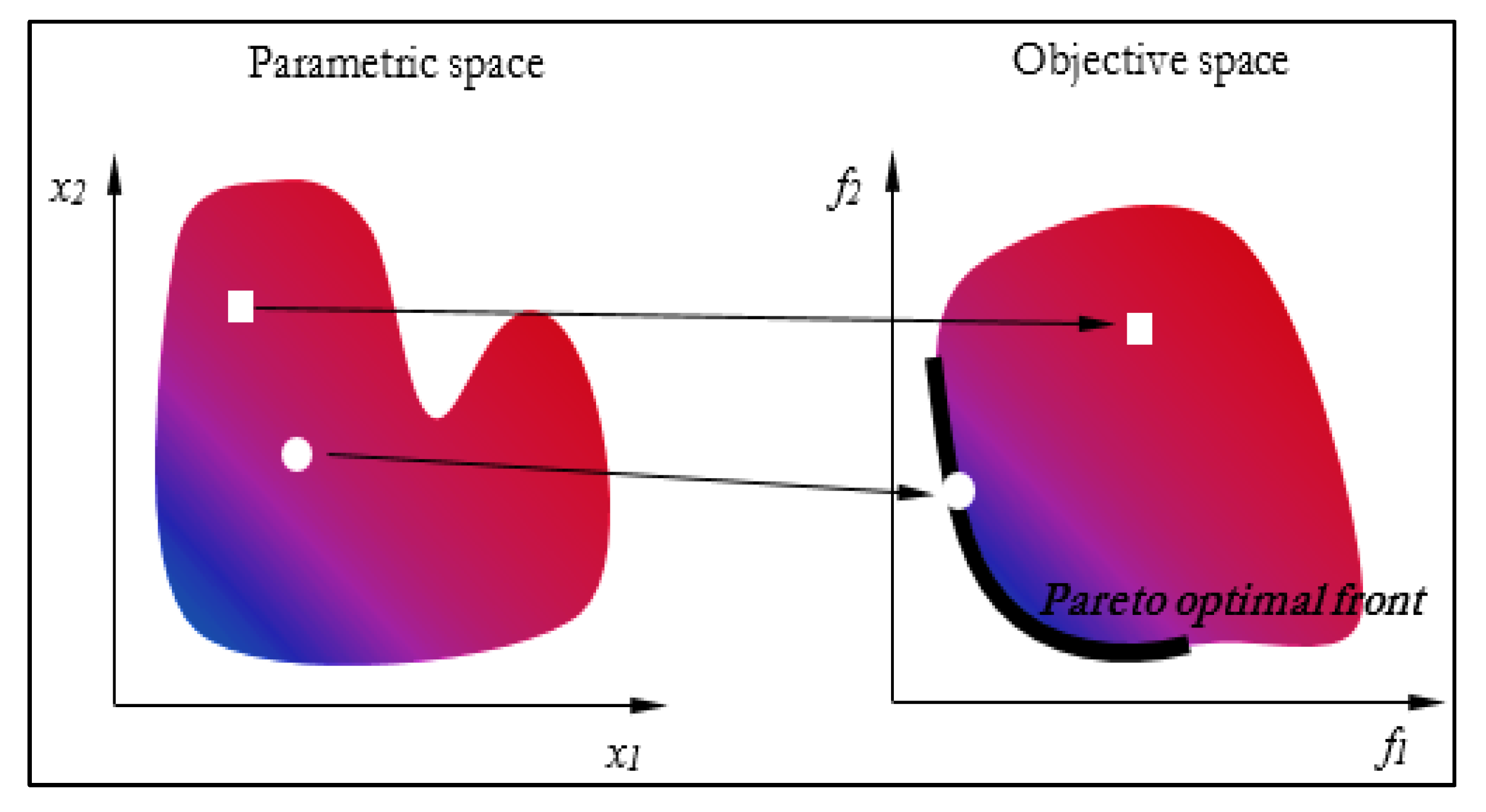
Any multi-objective optimization issue must be solved using the Pareto optimum set during the multi-objective optimization process. The search space (set of dominated solutions) and objective space (set of non-dominated solutions) are depicted in Figure 9. The Pareto optimum front describes the interaction between the objective space and search space.
4.6. Multi-Objective Generalized Normal Distribution Optimization (MOGNDO)
The proposed MOGNDO algorithm optimizer uses both the crowding distance (CD) mechanism and the elitist non-dominated sorting (NDS) method. The NDS consists of the following stages:
- Locating the non-dominated solution is the first step.
- The second step is the use of the NDS strategy.
- Performing non-dominated ranking (NDR) calculations on all non-dominated solutions.
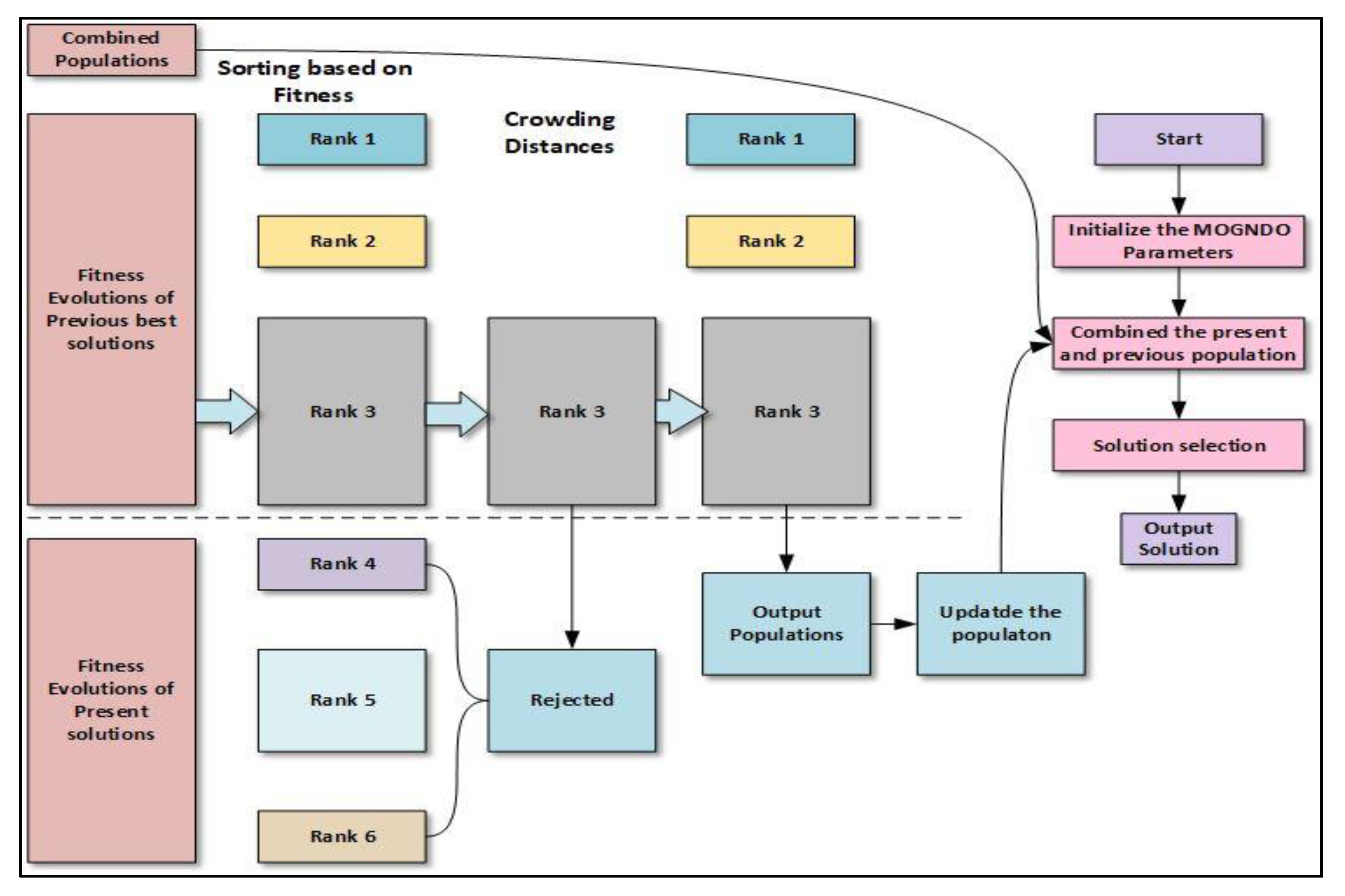
Between two fronts, the NDR process takes place. The first front’s solutions offer a “0” index because no solutions are dominated by them, but at least one solution from the first front dominates the second front’s solutions. A solution’s NDR is equal to the number of solutions that predominate it. The CD process is used to keep the created solutions diverse. The following is a definition of the CD mechanism:
where and are the maximum and minimum values of objective function. The diagrammatic illustration of an NDS-based approach is illustrated in Figure 10.
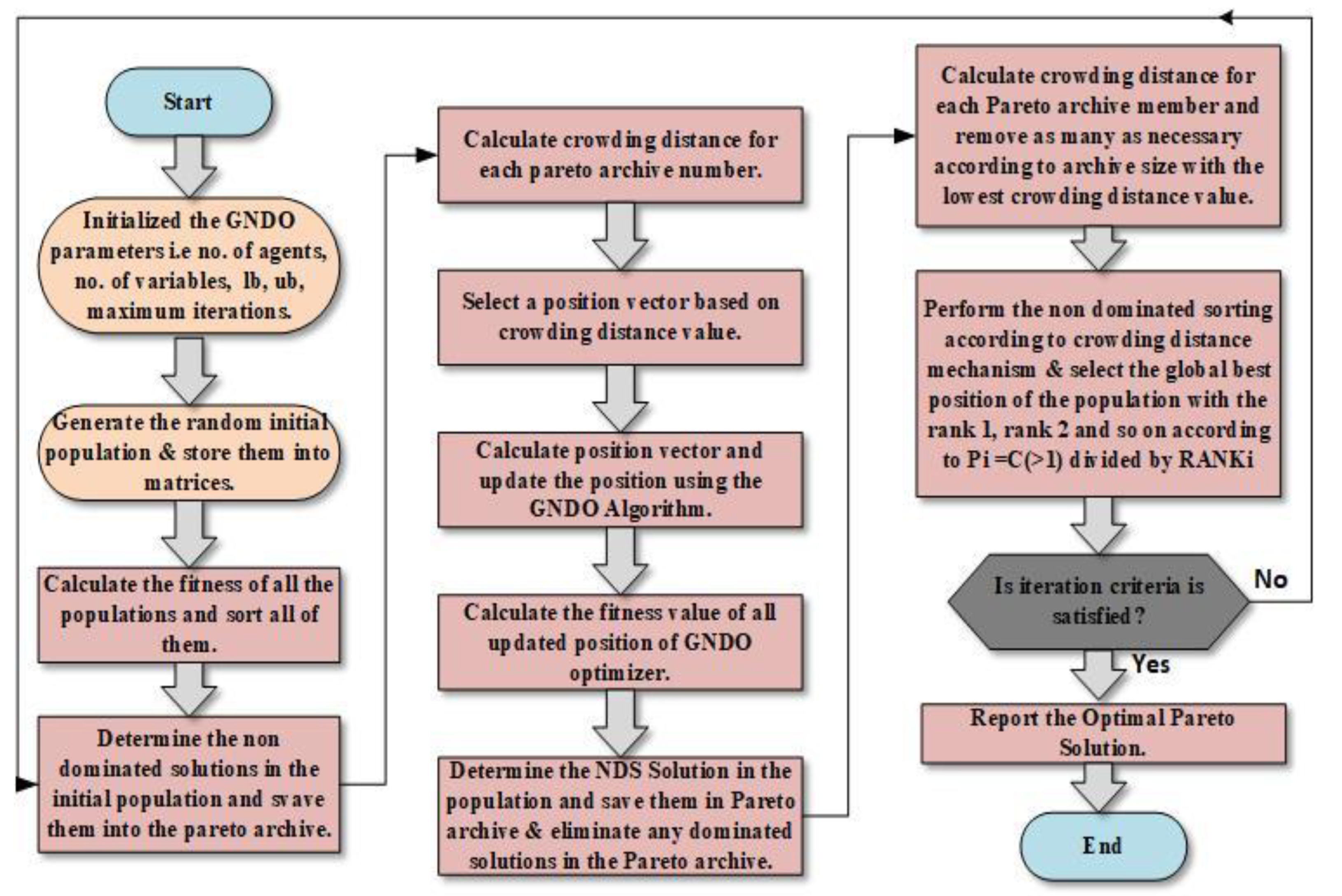
The MOGNDO algorithm’s pseudocode is displayed in Algorithm 1. The MOGNDO method begins by specifying the necessary inputs, such as population size (Np), termination criteria, the maximum number of generations, and the maximum number of iterations (Maxit). Then, each objective function in the objective space vector F for Po is evaluated using a randomly generated parent population Po in the feasible search space region S. Thirdly, Po is subjected to the elitist-based CD and NDS. Fourthly, Po is merged with a fresh population of Pj to create a population, Pi. This Pi is sorted using the CD and NDR data, as well as elitist non-dominance. To establish a new parent population, the best Np options are evaluated. The process is then repeated until the termination criteria are met. MOGNDO’s flowchart is displayed in Figure 11.
| Algorithm 1: Pseudocode of Multi-objective Generalized Normal Distribution Optimization (MOGNDO). |
| Step 1: Initially Generate population (Po) randomly in solution space (S) |
| Step 2: Evaluate objective space (F) for the generated population (Po) |
| Step 3: Sort the based on the elitist non-dominated sort method and find the non-dominated rank (NDR) and fronts |
| Step 4: Compute crowding distance (CD) for each front |
| Step 5: Update solutions (Pj) |
| Step 6: Merge Po and Pj to create Pi = Po U Pj |
| Step 7: For Pi perform Step 2 |
| Step 8: Based on NDR and CD sort Pi |
| Step 9: Replace Po with Pi for Np first members of Pi |
4.7. Constraint Handling Approach
The majority of engineering design issues in the actual world are multi-objective and highly nonlinearly constrained. To solve constrained MOPs, managing all constraints within their bounds is crucial. A static penalty technique is used in the MOGNDO algorithm because it transforms a constrained problem into an unconstrained problem, despite the literature survey giving various constrained handling approaches. This approach adds a significant penalty to the relevant goal function if a constraint is broken. The following is a presentation of the static penalty system:
where is the objective function to be optimized (here minimized), are design variables, are inequality constraints, are equality constraints, and is the tolerance in equality constraints.
4.8. Fuzzy Approach for the Multi-Objective Problem
The fuzzy membership approach can be used in multi-objective functions to identify the best compromising outcome out of all the non-inferior results. The fuzzy membership function uses a fuzzy membership function to keep track of the minimum and maximum values for each objective aim. Now, the membership function of the ith the objective is given as:
The standards of membership functions lie on the measure of (0–1) and display in the way that satisfies the function . Later, the decision-making function should be calculated as follows:
For non-inferior findings, the decision-making function can also be thought of as the normalized membership function, which displays the ordering of the undominated results. The end outcome is regarded as the best attainable compromise among all PFs, with a maximum value of .
5. Simulation Results, Analysis, and Comparative Study
This section discusses the outcomes of the MOGNDO algorithm, which optimized the optimal power flow with non-conventional and FACTS device problems with control variables. The initialization of the algorithm’s population size, archive size, the maximum number of iterations, and boundary condition for optimal power flow problems all came first. To identify the best optimal tradeoff points between multiple objective functions, the MOGNDO algorithm was then used to obtain the initial position and objective function values. Optimal power flow with non-conventional sources and FACTS devices were used to apply the MOGNDO algorithm’s performance, which was initially verified on eight unconstrained multi-objective problems. On a computer with 4 GB of RAM and a 3.20 GHz clock speed, the simulation was run using the MATLAB program. The benchmark functions for each unconstrained test were solved using 10 separate runs. The population size was set to 30, the maximum number of iterations was set to 100, and the archive size was set to 30 when the control parameters for the proposed MOGWO algorithm were first set. The performance measures for the MOGNDO algorithm, including Generational Distance (GD), Inversion Generational Distance (IGD), Spacing Metrics (SP), Diversity Metrics (DM), and Spread Metrics (SD), are covered in this section.
5.1. MOGNDO Results for Test Benchmark Problems
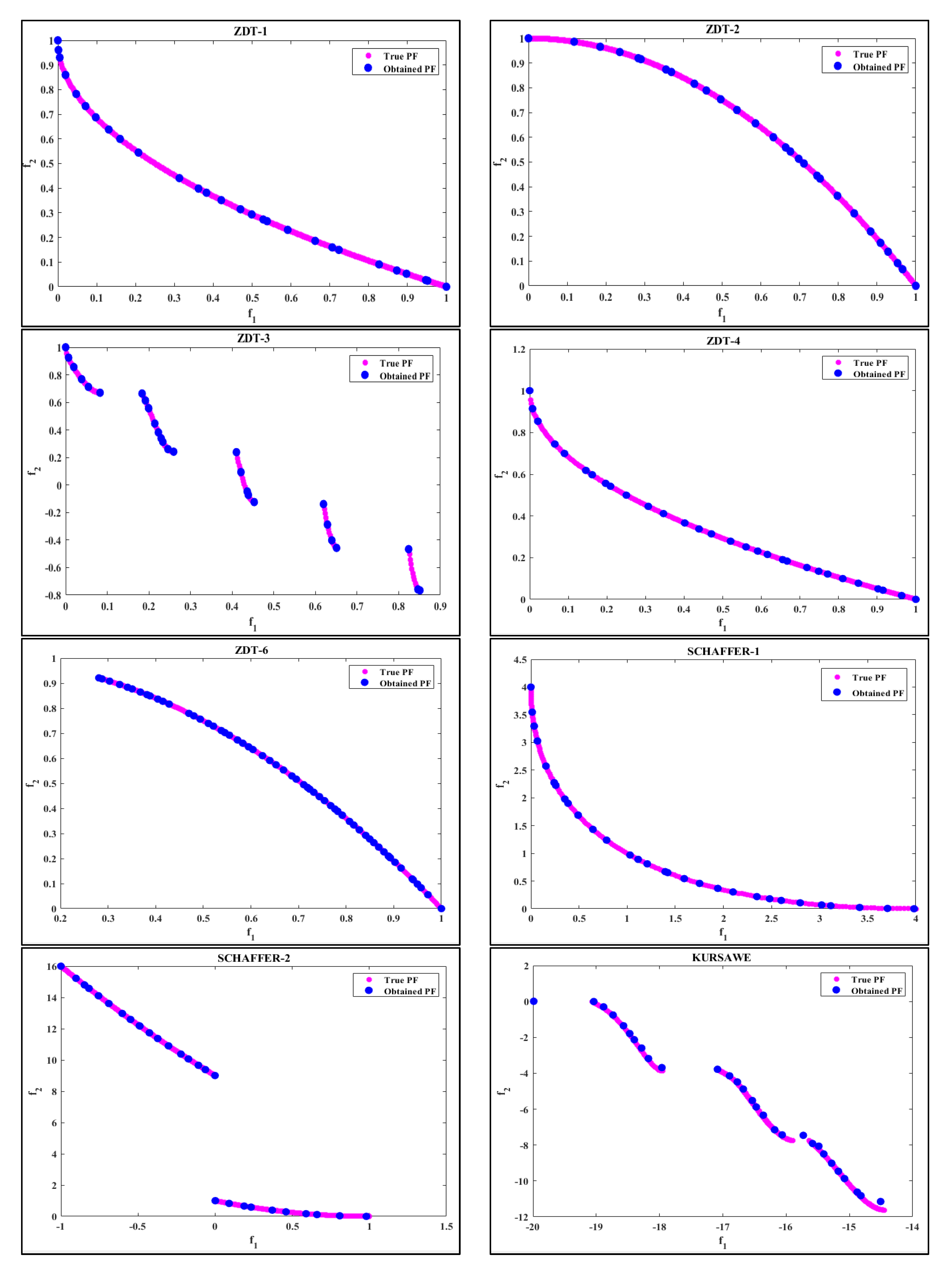
Before tackling real-world issues, the MOGNDO was used to evaluate the performance of the benchmark unconstraint test function provided in [26]. Eight benchmark unconstrained test functions—ZDT1, ZDT2, ZDT3, ZDT4, ZDT6, KURSAVE, SCHAFFER-1, and SCHAFFER-2 (Figure 12) were taken into account, and a thorough simulation was performed using the MOGNDO technique. Any algorithm’s control parameters are crucial to the resolution of the optimization problem. As a result, the number of populations was decided after conducting a comparative analysis that took into account various population sizes, while holding all other variables constant. Following careful consideration, the population size, maximum iterations, and archive size were chosen as 30, 100, and 30, respectively, for the unconstrained test benchmark functions. The MOGNDO algorithm’s performance was evaluated using performance metrics, such as Generational Distance (GD), Inversion Generational Distance (IGD), Spacing Metrics (SP), Diversity Metrics (DM), and Spread Metrics (SD), for convergence measurement. Table 3, Table 4, Table 5, Table 6 and Table 7 demonstrate that MOGNDO could achieve the best outcomes for all performance metrics, including Generational Distance (GD), Inversion Generational Distance (IGD), Spacing Metrics (SP), Diversity Metrics (DM), and Spread Metrics (SD), which cover convergence and solution accuracy. It follows that the suggested MOGNDO can provide the best convergence on all benchmark functions. The outcomes (archive solutions) of all eight test benchmark issues are displayed in Figure 1, Figure 2, Figure 3, Figure 4 and Figure 5. As can be shown, the MOGNDO method was capable of approximating the PF. By comparing the PF estimations, it can also be seen that the suggested MOGNDO could provide acceptable performance. Thus, it was determined that the MOGNDO algorithm is more suitable for the stochastic OPF problem with three FACTS devices and wind power plants.
5.2. Multi-Objectives OPF Problem with Wind Power Plants and Three FACTS Devices
The GNDO algorithm was used to address the stochastic OPF problem with wind power plants and three FACTS devices in this study. The solution to the optimum power flow problem was evaluated in parallel using newly created algorithms, such as the Multi-Verse Optimization (MVO), the Sine-Cosine Algorithm (SCA) [27], the Grey Wolf Optimization (GWO), the Moth Fame Optimization (MFO), the Ant Lion Optimization (ALO) [28], and Ion Motion Algorithms (IMA) [29]. The proposed approach was demonstrated using a modified IEEE-30 bus infrastructure with wind power plants and FACTS devices. Table 1 lists the major characteristics of the customized IEEE-30 bus framework. The following are two scenarios:
- Scenario-1 (Solo objective OPF with wind power plants and FACTS devices)
- Scenario-2 (Multi-objective OPF with wind power plants and FACTS devices)
As shown in Table 8, there were a total of thirteen different test scenarios to evaluate. In this section, the results of case studies using various metaheuristics methodologies are tabulated and presented. The first six case studies are for single-objective optimization, while the latter seven are multi-objective optimization problems that include non-conventional sources of energy resources, as well as optimal FACTS device sizes and locations. The search agent value was set to 40, and each algorithm underwent 500 iterations of analysis. Please refer to the original research for a detailed discussion of those procedures. Table 4 shows the parameter settings for these methods.
5.3. Scenario-1 (Single Objective OPF with Wind Power Plants and FACTS Devices)
With the use of GNDO, MVO, ALO, SCA, and IMO methods, all of the objective goals indicated in the mathematical formulation were simultaneously handled as solo objective optimization issues. The limitations of all control variables, as well as proper FACTS device locations and sizing, are listed below. From case 1 to case 6, the outcomes of objective functions are tabulated in Table 9, Table 10 and Table 11, with the best minimum values containing five different recent techniques.
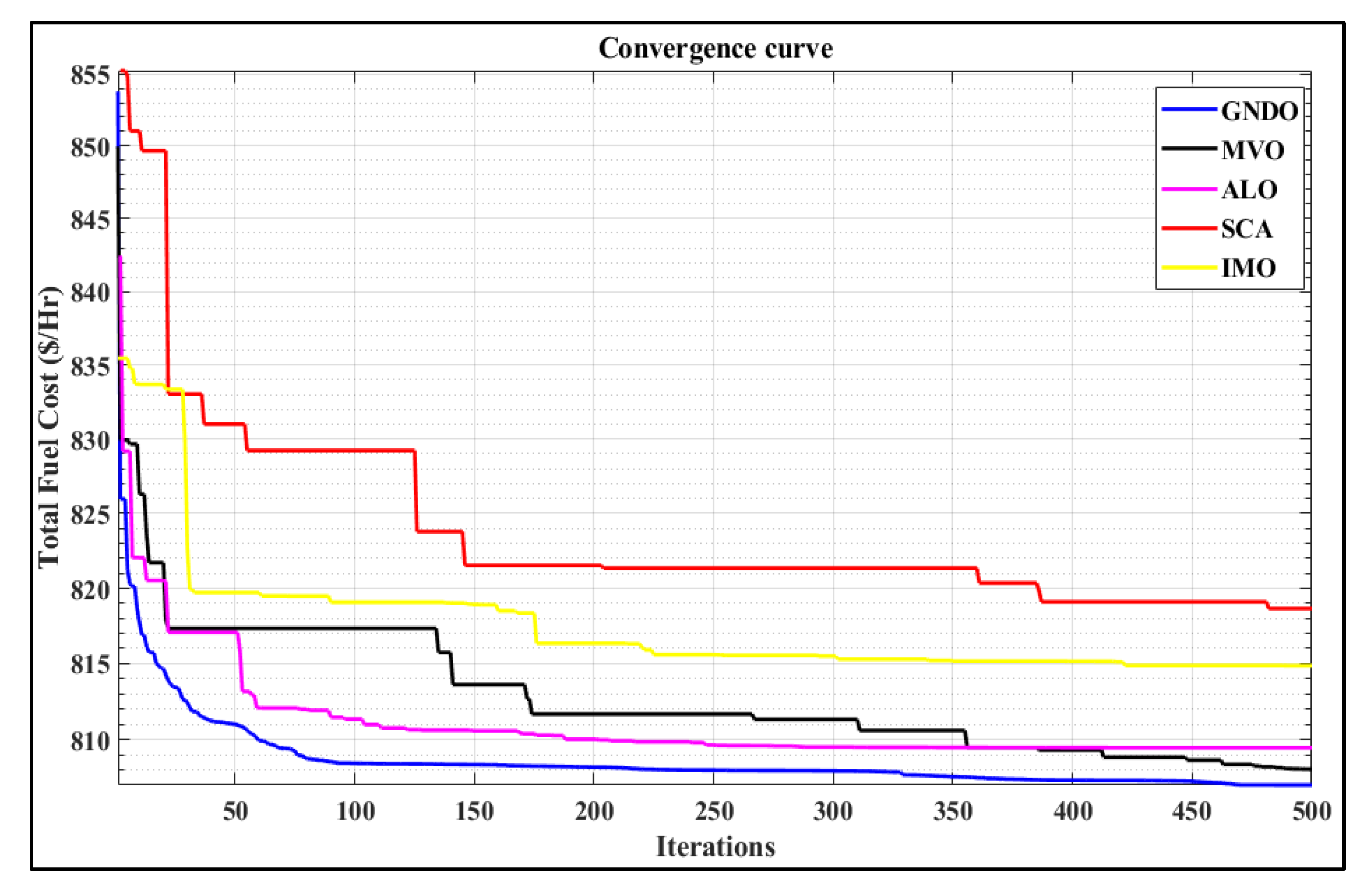
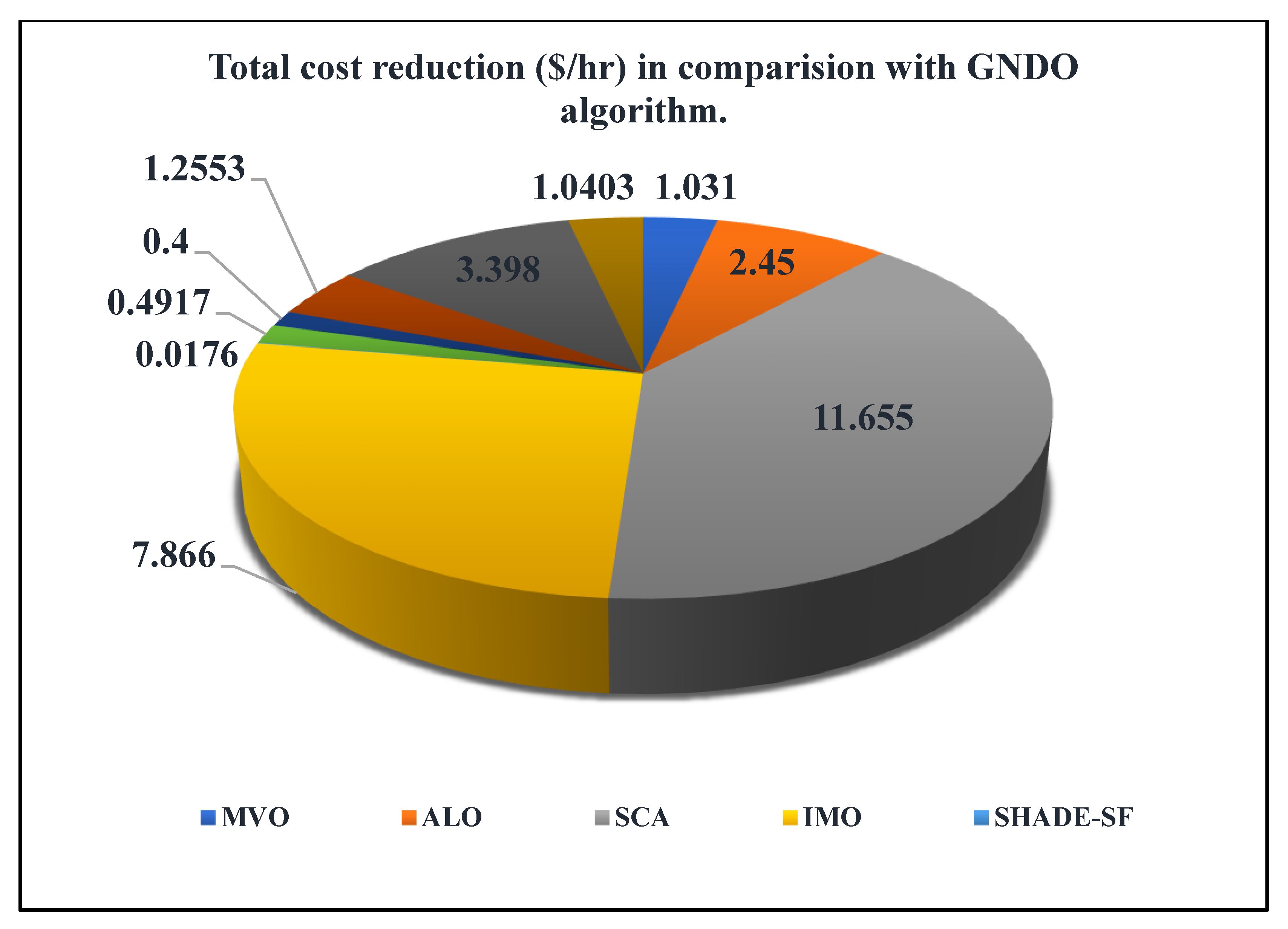
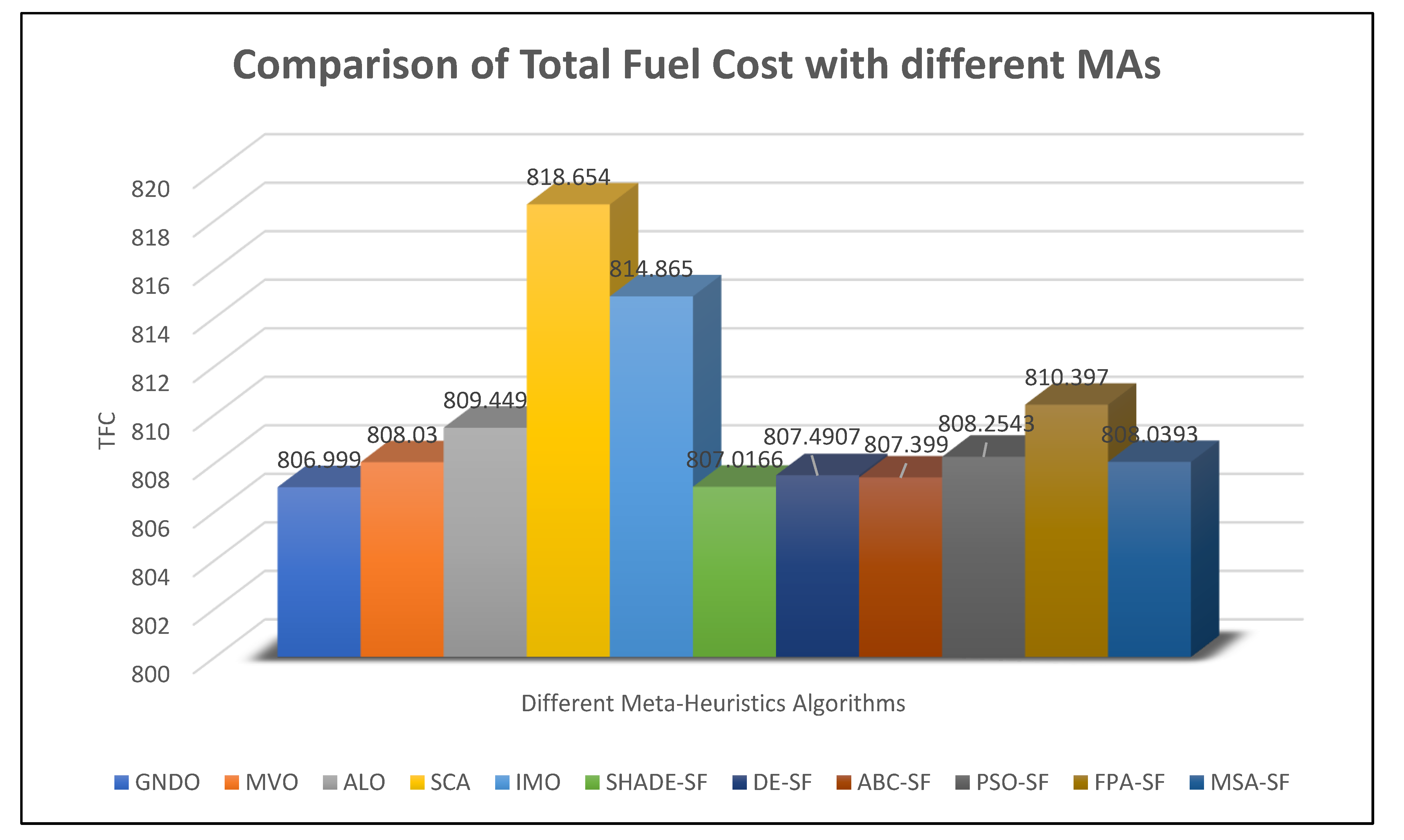
The overall fuel cost with GNDO, which included the two non-conventional sources of power plants and optimal placement of FACTS devices, was 806.999 $/h, which was the best in comparison with the other cited algorithm shown in Table 9. The reductions in TFC in comparison with MVO, ALO, SCA, IMO, SHADE-SF, DE-SF, ABC-SF, PSO-SF, FPA-SF, and MSA-SF were 1.031 $/h, 1.031 $/h, 2.45 $/h, 11.655 $/h 7.866 $/h, 0.0176 $/h, 0.4917 $/h, 0.4 $/h, 1.2553 $/h, 3.398 $/h, and 1.0403 $/h, respectively. This demonstrated the GNDO algorithm’s superiority over other cited metaheuristics algorithms.
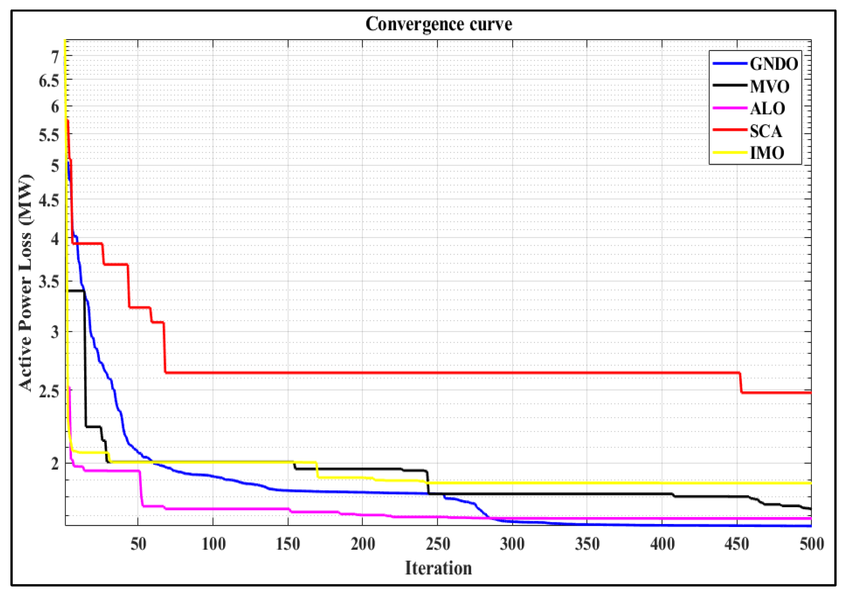
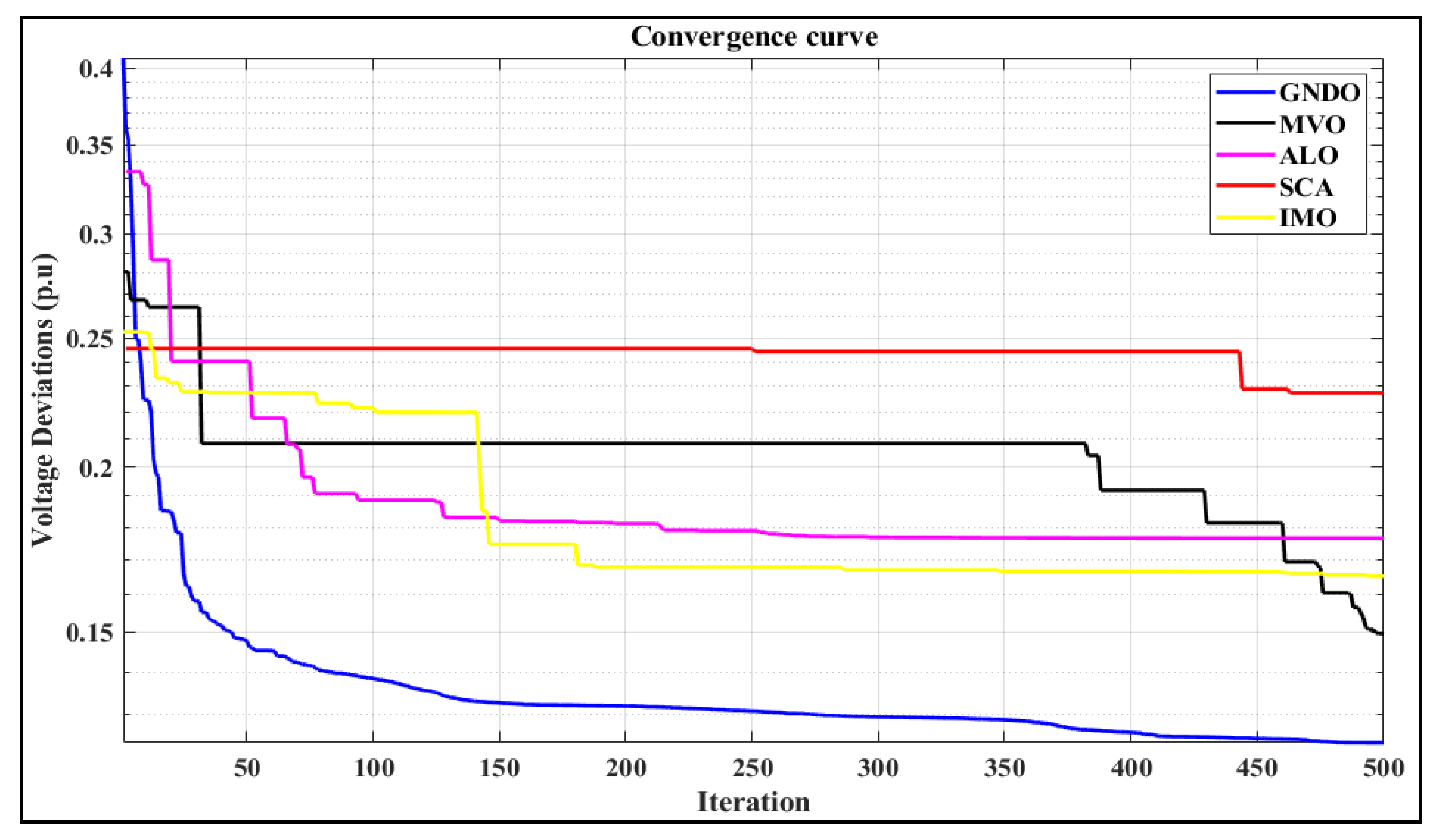
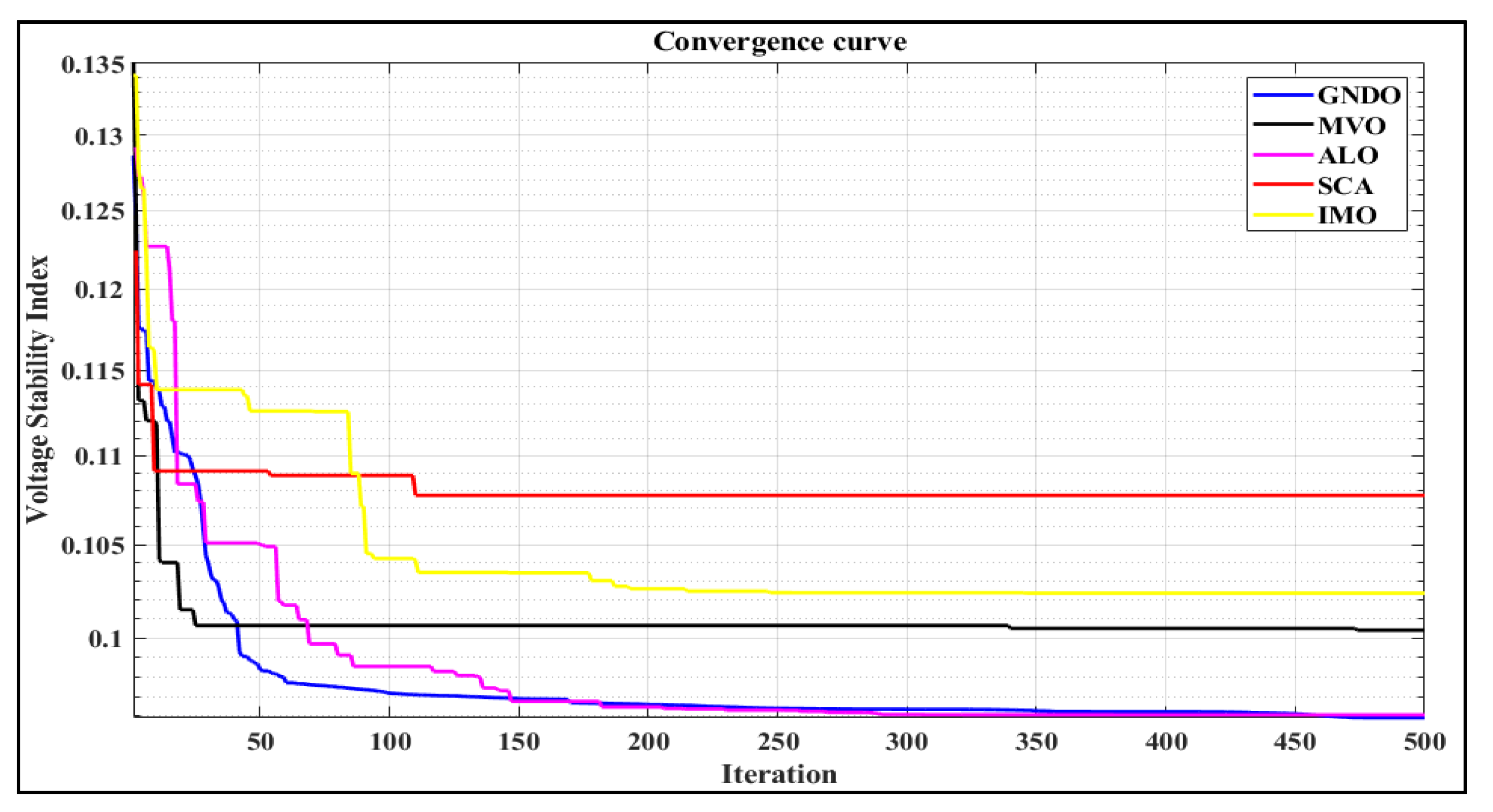
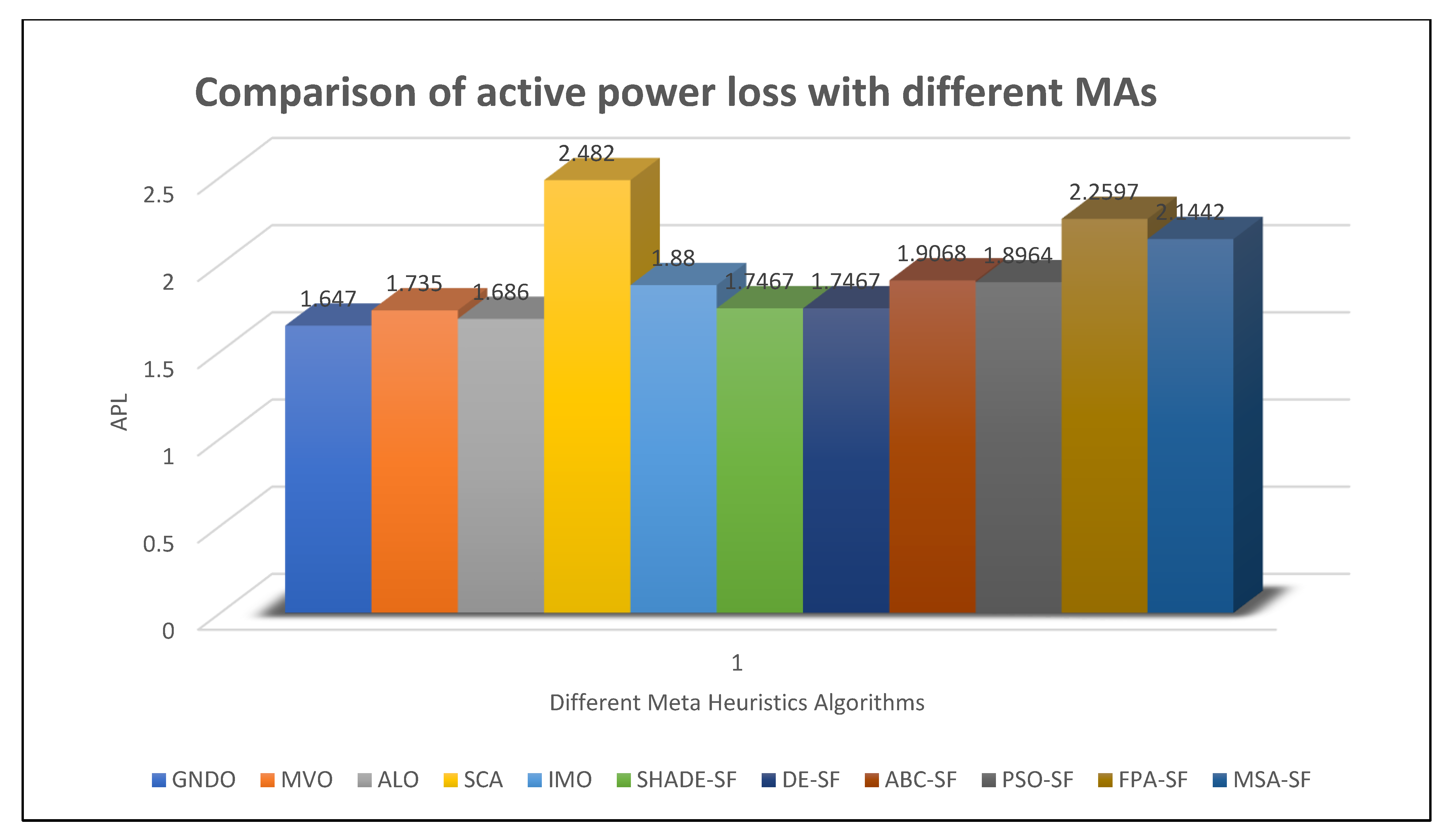
Figure 13 illustrates the convergence traits of the TFC minimization. Similar convergence traits for APL, voltage deviations, and VSI are depicted in Figure 14, Figure 15 and Figure 16. Figure 17 also displays a comparison of the fuel cost decrease with various algorithms. In example 2, the GNDO method resulted in a pollutant gas emission of 0.138 tons per hour. In instance 3, the APL of the various transmission lines using the GNDO approach was 1.647 MW. The APL was 0.088 MW, 0.039 MW, 0.835 MW, 0.233 MW, 0.0997 MW, 0.0997 MW, 0.2598 MW, 0.2494 MW, 0.6127 MW, and 0.4972 MW less compared to MVO, ALO, SCA, IMO, SHADE-SF, DE-SF, ABC-SF, PSO-SF, and MSA-SF, respectively. A crucial factor for the grid’s ability to operate reliably was the voltage divergence of each bus from 1.0 per unit. Therefore, in scenario 4, the moth flame algorithm produced the lowest voltage variation (0.124 p.u), making it the best of the five optimization methods. The VSI, sometimes referred to as the L max index, varied between zero (no load) and one (voltage collapse). Therefore, in case 5, 0.096 was the lowest value for the L max index. In scenario 6, the overall gross fuel cost using the GNDO method was 1120.996 dollars per hour. It is interesting to note here that in Table 12, the total gross fuel cost of the proposed GNDO was more than the SHADE-SF, which further enforces the narrative of the “No free lunch theorem,” which states that no algorithm gives the best result in every problem.
Figure 18 and Figure 19 provide comparison charts with the minimizing of APL and overall fuel cost. The results of the simulations were compared to those of the most recent algorithms, including MVO, ALO, SCA, IMO, and other mentioned optimization approaches. It was found that the proposed method of Generalized Normal Distribution Optimization methodology produced superior results.
5.4. Scenario-2 (Multi-Objective OPF with Non-Conventional Sources Energy Resources)
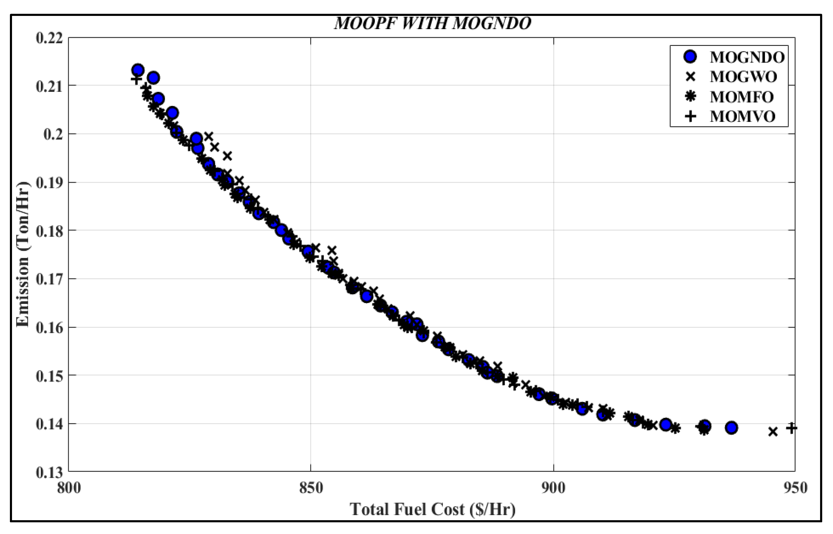
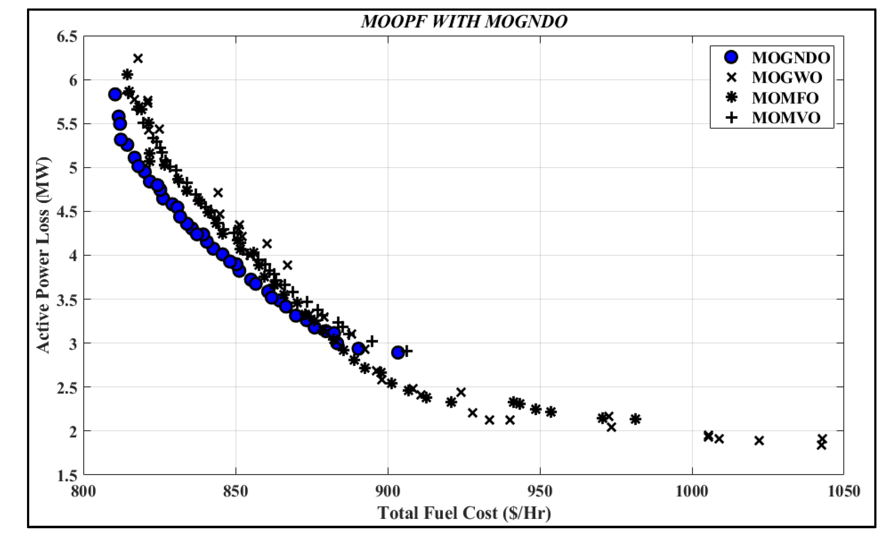
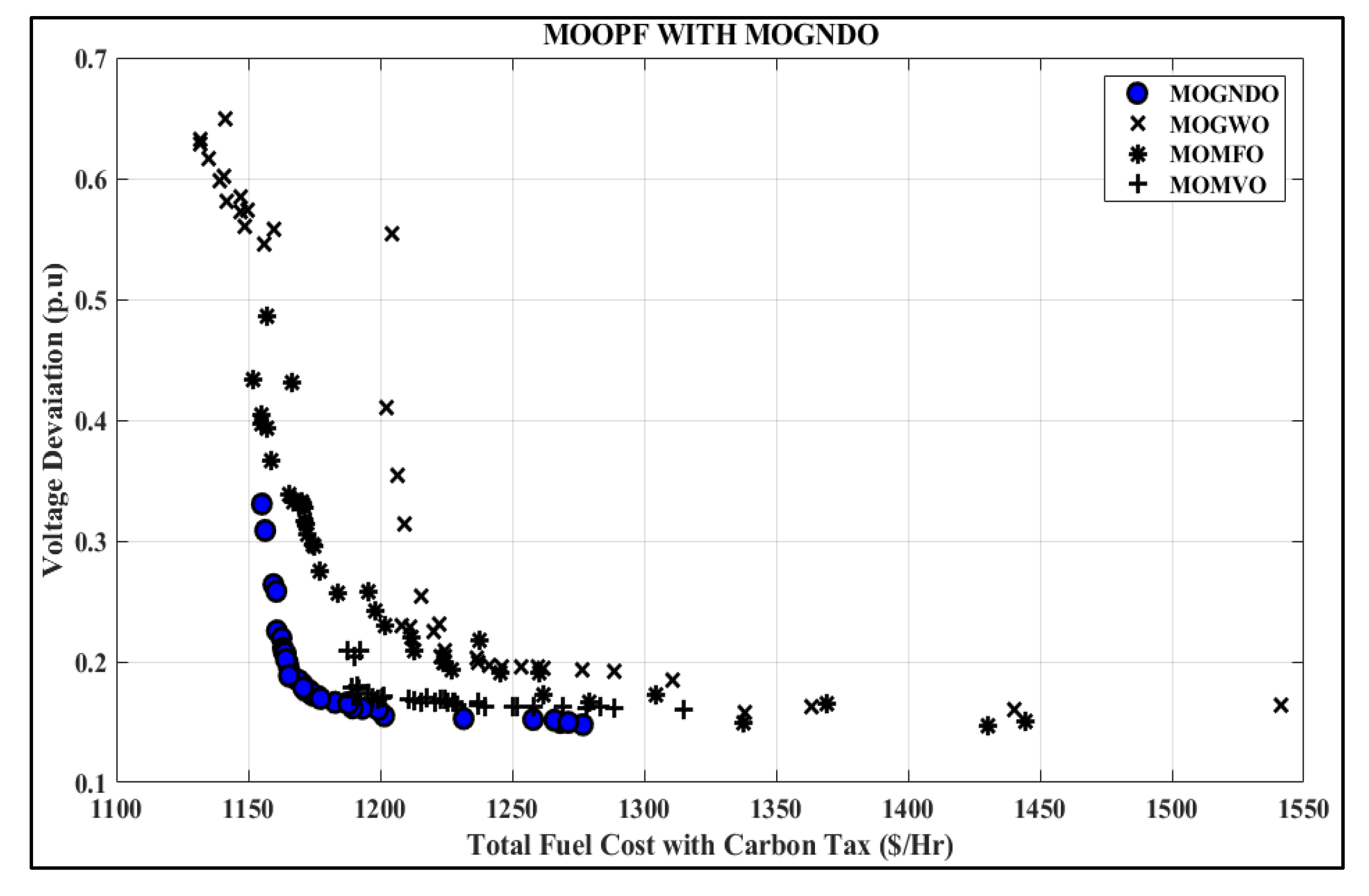
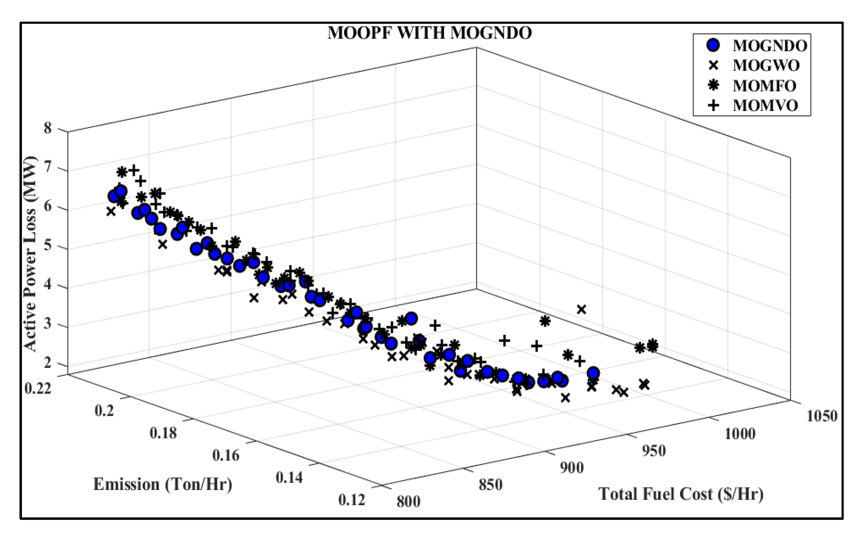
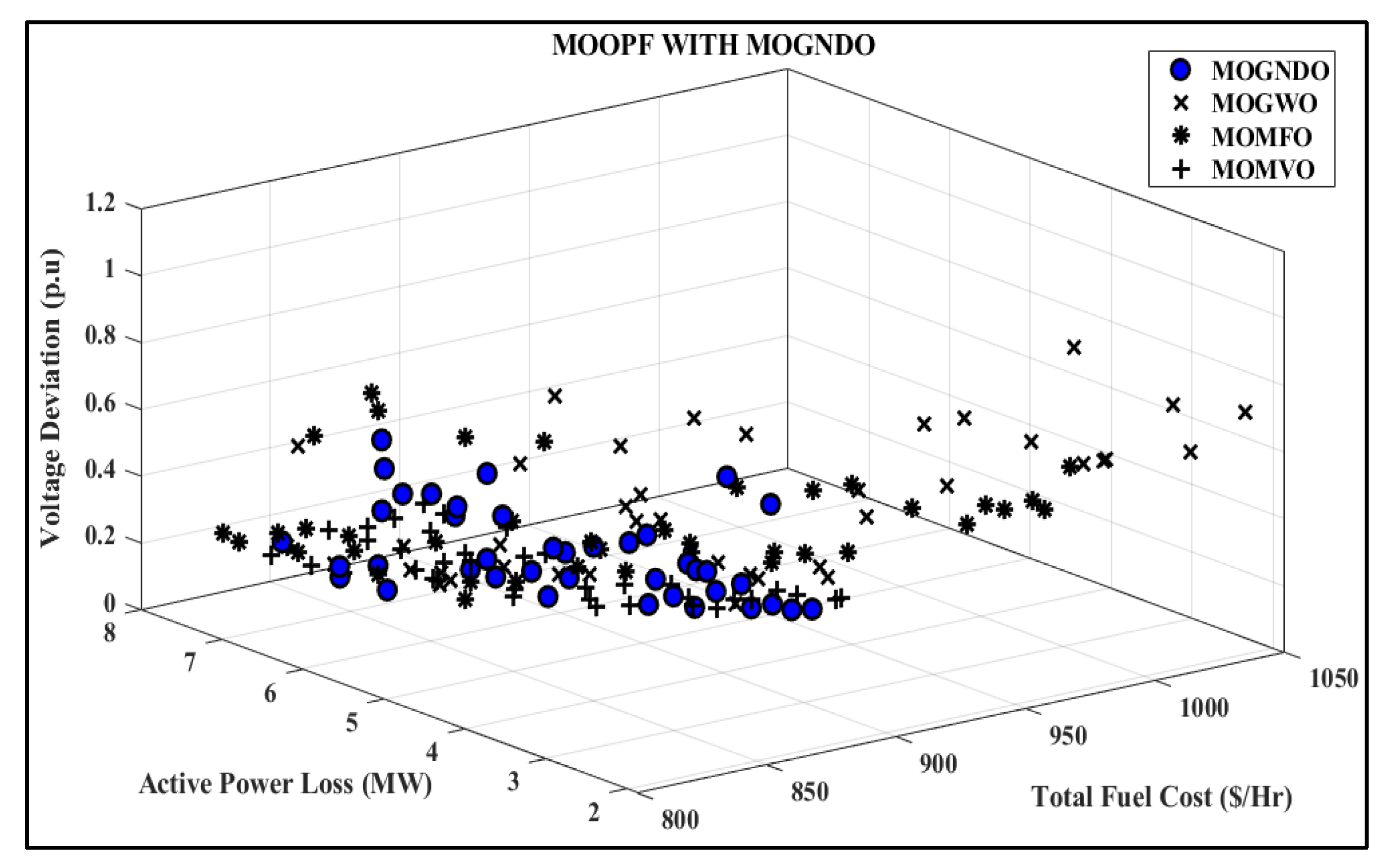
In this case, two, three, and four objectives were simultaneously optimized using the Multi-Objective Generalized Normal Distribution Optimization (MOGNDO) algorithm technique. In multi-objective optimization, the non-dominated sorting optimization technique is used to simultaneously find solutions for numerous objectives. To find the PF for the modified IEEE 30-bus architecture, 30 non-dominate solutions are retained. The scenarios in cases 7 through 10 are thought of as two-objective optimization cases. Three-objective optimization problems are what are known as cases 11 and 12. Contrarily, case 13 is referred to as a set of four problems involving objective optimization. Among all the Pareto archives, the best compromising solution was found using the fuzzy decision-making method. For cases 7 through 13, the most optimal compromise solutions using the proposed MOGNDO algorithm and other cited metaheuristics techniques are shown in boldface and stated in Table 13, Table 14, Table 15 and Table 16. The best PFs of TFC and pollution minimization for case 7 are shown in Figure 20, utilizing various metaheuristics techniques. Likewise with case 7, case 8’s PF with two goal optimizations resulted in APL and TFC, which are depicted in Figure 21. Figure 22 shows the PF of the TFC with the carbon tax and voltage deviation minimization. In scenario 11, Figure 23 shows the three objectives PFs for minimizing APL, TFC, and toxic gas emanations. Figure 24 depicts the PF for the minimization of voltage variation, APL, and TFC, using various algorithms.
The MOGNDO methodology was one of the finest methods for finding the best solutions to the multi-objective OPF problem that integrated with wind power plants and the appropriate placement of FACTS devices, according to the tabulated data.
6. Conclusions
The optimal location and size of FACTS devices in this study, as well as single- and multi-objective optimal power flow (MOOPF) concerned coal-based and wind power plants, which were all addressed by the solution technique. Different probability density functions were used to express inconsistencies in unconventional resource availability. The method for integrating each unit was described in detail. When utilizing non-conventional sources of energy sources and FACTS devices, single objectives were optimized, such as generation cost, toxic gas emanation, voltage deviation, active loss, and VSI. A multi-objective form of the OPF problem was looked into in light of the current situation of the electric network. The outcomes were contrasted with a recently created optimization strategy. Based on the results, it can be said that the proposed MOGNDO outperformed existing algorithms in terms of convergence, and delivered higher quality and more usable solutions for each situation involving optimal power flow. All of the results point to the suggested technique’s significant advantage in obtaining the best solutions to OPF issues with one or more objectives. Finally, it was shown that by integrating wind farms with FACTS devices utilizing a non-dominated sorting technique, MOGNDO could be successfully employed to address small and large optimal power flow challenges. Based on the extensive analysis of the proposed MOGNDO, the following can be summarized as its advantages—
- Randomization in MOGNDO includes the diversity of the Pareto front being enhanced, since all solutions in the first dominated front will have an equal chance of being selected, and multi-objectives are made uniformly significant while performing local exploration.
- MOGNDO can deal with large-scale search spaces and is less dependent on problem characteristics. Moreover, these algorithms are capable of estimating multiple points in the search domain simultaneously, due to their population-based nature.
- MOGNDO strikes a good balance between exploitation and exploration, providing powerful searchability for finding the optimum solution
- MOGNDO is superior in terms of the balance of diversity and convergence, the distribution of PF, and better convergence.
Author Contributions
Conceptualization, S.B.P., J.V. and M.M.; Methodology, S.B.P., J.V., M.M. and T.K.M.; Software, T.K.M. and P.J.; Validation, S.B.P., M.M. and T.K.M.; Formal analysis, J.V., M.M. and T.K.M.; Investigation, S.B.P.; Resources, P.J.; Data curation, J.V. and P.J.; Writing—original draft, S.B.P., J.V., M.M., T.K.M. and P.J.; Writing—review & editing, S.B.P.; Visualization, T.K.M. and P.J.; Supervision, S.B.P.; Funding acquisition, M.M. All authors have read and agreed to the published version of the manuscript.
Funding
This work was supported by the project SP2022/60 Applied Research in the Area of Machines and Process Control, which is supported by the Ministry of Education, Youth and Sports, in the Czech Republic.
Institutional Review Board Statement
Not applicable.
Informed Consent Statement
Not applicable.
Data Availability Statement
The data presented in this study are available in the article.
Conflicts of Interest
The authors declare no conflict of interest.
Abbreviations
| Acronyms | |
| OPF | Optimal Power Flow |
| Mas | Meta Heuristics Algorithms |
| MOGNDO | Multi-Objective Generalized Normal Distribution Optimization |
| TG | Thermal Generating unit |
| WG | Wind Generation |
| ISO | Independent System Operator |
| Probability Density Function | |
| BCS | Best Compromise Solution |
| MOMFO | Multi-Objective Moth Flame Optimization |
| MOOPF | Multi-Objective Optimal Power Flow |
| SHADE-SF | Success History-based Adaptive Differential Evolution using Superiority of Feasible solutions method |
| DE-SF | Differential Evolution using Superiority of Feasible solutions method |
| ABC-SF | Artificial Bee Colony using Superiority of Feasible solutions method |
| PSO-SF | Particle Swarm Optimization using Superiority of Feasible solutions method |
| FPA-SF | Flower Pollination Algorithm using Superiority of Feasible solutions method |
| MSA-SF | Moth Swarm Algorithm using Superiority of Feasible solutions method |
| TFC | Total Fuel Cost |
| APL | Active power Loss |
| VSI | Voltage Stability Index |
| Nomenclature | |
| Price constants for ith coal-based power plants. | |
| Toxic gas emanation constants concerning the ith coal-based units. | |
| Direct cost constant | |
| Scheduled power of the wind unit. | |
| Reserve cost coefficient regarding wind unit | |
| Penalty cost coefficient of wind unit | |
| Accessible power from the wind unit | |
| Specified output power from the wind unit | |
| Wind energy probability density function for the wind unit. | |
| and | Cut-in, rated, and cut-out wind velocity of the turbine respectively |
| Rated value of the generated output of the wind turbine | |
| Degree of series compensation | |
| Line inductive reactance linking buses and | |
| Resistance of the line linking buses and | |
| and | Bus voltage magnitudes linking buses and . |
| and | Phase angles of the linking buses and |
| and | Conductance and susceptance of the line linking buses and . |
| Number of load (PQ) buses | |
| pu voltage level of th bus. | |
| and | Generation and dispatch at th bus |
| Number of buses | |
| and | Sub-matrices of |
| Variance in phase angles of voltage among bus and bus | |
| and | Real and VAR power demand respectively at th bus |
| and | Real and VAR outputs respectively of th bus by either unit (coal-based or non-conventional) as applicable |
| and | Conductance and susceptance between bus and bus |
References
- Joshi, M.; Ghadai, R.K.; Madhu, S.; Kalita, K.; Gao, X.-Z. Comparison of NSGA-II, MOALO and MODA for Multi-Objective Optimization of Micro-Machining Processes. Materials 2021, 14, 5109. [Google Scholar] [CrossRef] [PubMed]
- Cao, B.; Li, M.; Liu, X.; Zhao, J.; Cao, W.; Lv, Z. Many-objective deployment optimization for a drone-assisted camera network. IEEE Trans. Netw. Sci. Eng. 2021, 8, 2756–2764. [Google Scholar] [CrossRef]
- Liang, X.; Luo, L.; Hu, S.; Li, Y. Mapping the knowledge frontiers and evolution of decision making based on agent-based modeling. Knowl.-Based Syst. 2022, 250, 108982. [Google Scholar] [CrossRef]
- Zhang, K.; Wang, Z.; Chen, G.; Zhang, L.; Yang, Y.; Yao, C.; Wang, J.; Yao, J. Training effective deep reinforcement learning agents for real-time life-cycle production optimization. J. Pet. Sci. Eng. 2022, 208, 109766. [Google Scholar] [CrossRef]
- Ganesh, N.; Ghadai, R.K.; Bhoi, A.K.; Kalita, K.; Gao, X.-Z. An intelligent predictive model-based multi-response optimization of EDM process. Comput. Model. Eng. Sci. 2020, 124, 459–476. [Google Scholar] [CrossRef]
- Ghadai, R.K.; Kalita, K.; Gao, X.-Z. Symbolic regression metamodel based multi-response optimization of EDM process. FME Trans. 2020, 48, 404–410. [Google Scholar] [CrossRef]
- Cao, B.; Zhang, W.; Wang, X.; Zhao, J.; Gu, Y.; Zhang, Y. A memetic algorithm based on two_Arch2 for multi-depot heterogeneous-vehicle capacitated arc routing problem. Swarm Evol. Comput. 2021, 63, 100864. [Google Scholar] [CrossRef]
- Liu, Y.; Zhang, Z.; Liu, X.; Wang, L.; Xia, X. Ore image classification based on small deep learning model: Evaluation and optimization of model depth, model structure and data size. Miner. Eng. 2021, 172, 107020. [Google Scholar] [CrossRef]
- Ullah, Z.; Wang, S.; Radosavljevic, J.; Lai, J. A solution to the optimal power flow problem considering WT and PV generation. IEEE Access 2019, 7, 46763–46772. [Google Scholar] [CrossRef]
- Elattar, E.E. Optimal power flow of a power system incorporating stochastic wind power based on modified moth swarm algorithm. IEEE Access 2019, 7, 89581–89593. [Google Scholar] [CrossRef]
- Man-Im, A.; Ongsakul, W.; Singh, J.G.; Madhu, M.N. Multi-objective optimal power flow considering wind power cost functions using enhanced PSO with chaotic mutation and stochastic weights. Electr. Eng. 2019, 101, 699–718. [Google Scholar] [CrossRef]
- Salkuti, S.R. Optimal power flow using multi-objective glowworm swarm optimization algorithm in a wind energy integrated power system. Int. J. Green Energy 2019, 16, 1547–1561. [Google Scholar] [CrossRef]
- Kathiravan, R.; Kumudini Devi, R.P. Optimal power flow model incorporating wind, solar, and bundled solar-thermal power in the restructured Indian power system. Int. J. Green Energy 2017, 14, 934–950. [Google Scholar] [CrossRef]
- Duman, S.; Rivera, S.; Li, J.; Wu, L. Optimal power flow of power systems with controllable wind-photovoltaic energy systems via differential evolutionary particle swarm optimization. Int. Trans. Electr. Energy Syst. 2020, 30. [Google Scholar] [CrossRef]
- Duman, S.; Li, J.; Wu, L.; Guvenc, U. Optimal power flow with stochastic wind power and FACTS devices: A modified hybrid PSOGSA with chaotic maps approach. Neural Comput. Appl. 2020, 32, 8463–8492. [Google Scholar] [CrossRef]
- Biswas, P.P.; Suganthan, P.N.; Qu, B.Y.; Amaratunga, G.A.J. Multiobjective economic-environmental power dispatch with stochastic wind-solar-small hydro power. Energy 2018, 150, 1039–1057. [Google Scholar] [CrossRef]
- Chen, M.-R.; Zeng, G.-Q.; Lu, K.-D. Constrained multi-objective population extremal optimization based economic-emission dispatch incorporating renewable energy resources. Renew. Energy 2019, 143, 277–294. [Google Scholar] [CrossRef]
- Chang, Y.-C.; Lee, T.-Y.; Chen, C.-L.; Jan, R.-M. Optimal power flow of a wind-thermal generation system. Int. J. Electr. Power Energy Syst. 2014, 55, 312–320. [Google Scholar] [CrossRef]
- Saha, A.; Bhattacharya, A.; Das, P.; Chakraborty, A.K. A novel approach towards uncertainty modeling in multiobjective optimal power flow with renewable integration. Int. Trans. Electr. Energy Syst. 2019, 29. [Google Scholar] [CrossRef]
- Biswas, P.P.; Suganthan, P.N.; Amaratunga, G.A.J. Optimal power flow solutions incorporating stochastic wind and solar power. Energy Convers. Manag. 2017, 148, 1194–1207. [Google Scholar] [CrossRef]
- Ben Hmida, J.; Chambers, T.; Lee, J. Solving constrained optimal power flow with renewables using hybrid modified imperialist competitive algorithm and sequential quadratic programming. Electr. Power Syst. Res. 2019, 177, 105989. [Google Scholar] [CrossRef]
- Pandya, S.; Jariwala, H.R. Single- and multiobjective optimal power flow with stochastic wind and solar power plants using moth flame optimization algorithm. Smart Sci. 2022, 10, 77–117. [Google Scholar] [CrossRef]
- Biswas, P.P.; Arora, P.; Mallipeddi, R.; Suganthan, P.N.; Panigrahi, B.K. Optimal placement and sizing of FACTS devices for optimal power flow in a wind power integrated electrical network. Neural Comput. Appl. 2021, 33, 6753–6774. [Google Scholar] [CrossRef]
- Wolpert, D.H.; Macready, W.G. No free lunch theorems for optimization. IEEE Trans. Evol. Comput. 1997, 1, 67–82. [Google Scholar] [CrossRef] [Green Version]
- Zhang, Y.; Jin, Z.; Mirjalili, S. Generalized normal distribution optimization and its applications in parameter extraction of photovoltaic models. Energy Convers. Manag. 2020, 224, 113301. [Google Scholar] [CrossRef]
- Kumar, S.; Jangir, P.; Tejani, G.G.; Premkumar, M.; Alhelou, H.H. MOPGO: A new physics-based multi-objective plasma generation optimizer for solving structural optimization problems. IEEE Access 2021, 9, 84982–85016. [Google Scholar] [CrossRef]
- Mirjalili, S. SCA: A Sine Cosine Algorithm for solving optimization problems. Knowl. Based Syst. 2016, 96, 120–133. [Google Scholar] [CrossRef]
- Mirjalili, S. The ant lion optimizer. Adv. Eng. Softw. 2015, 83, 80–98. [Google Scholar] [CrossRef]
- Javidy, B.; Hatamlou, A.; Mirjalili, S. Ions motion algorithm for solving optimization problems. Appl. Soft Comput. 2015, 32, 72–79. [Google Scholar] [CrossRef]
Figure 1.
Adapted IEEE 30-bus scheme with power units and FACTS policies [23].
Figure 1.
Adapted IEEE 30-bus scheme with power units and FACTS policies [23].

Figure 2.
Weibull PDF (bus 5).

Figure 3.
Weibull PDF (bus 11).

Figure 4.
Basic Structure and model of TCSC [23].
Figure 4.
Basic Structure and model of TCSC [23].

Figure 5.
Model of TCP [23].
Figure 5.
Model of TCP [23].

Figure 6.
Basic structure and model of SVC [23].
Figure 6.
Basic structure and model of SVC [23].

Figure 7.
The framework of the proposed GNDO [25].
Figure 7.
The framework of the proposed GNDO [25].

Figure 8.
The pseudocode of GNDO [25].
Figure 8.
The pseudocode of GNDO [25].

Figure 9.
Objective space and search space in the multi-objective optimization problem.

Figure 10.
The procedure of the non-dominated sorting approach.

Figure 11.
Flowchart of MOGNDO algorithm.

Figure 12.
Best Pareto optimal front obtained of unconstrained test functions by MOGNDO algorithm.

Figure 13.
Convergence characteristics of TFC minimization.

Figure 14.
Convergence characteristics of APL minimization.

Figure 15.
Convergence characteristics of voltage deviation minimization.

Figure 16.
Convergence characteristics of VSI minimization.

Figure 17.
Comparison of the TFC reduction ($/h) with other algorithms.

Figure 18.
Comparison chart for TFC minimization with different algorithms.

Figure 19.
Comparison chart for APL minimization with different algorithms.

Figure 20.
PF of TFC and emission minimization.

Figure 21.
PF of TFC and APL minimization.

Figure 22.
PF of TFC with a carbon tax and voltage deviation minimization.

Figure 23.
PF of TFC, emission, and APL minimization with different algorithms.

Figure 24.
PF of TFC, APL, and voltage deviation minimization with different algorithms.


Table 1.
Test system key features for analysis.
| Particulars | Quantity | Details |
|---|---|---|
| Total buses | 30 | [23] |
| Total branches | 41 | [23] |
| Coal-based generators (TG1; TG2; TG3; TG4) | 4 | Buses: 1 (swing), 2, 8 and 13 |
| Wind generators (WG1; WG2) | 2 | Bus-5 and Bus-11 |
| Tap changing transformers | 4 | Branches: 11, 12, 15 and 36 |
| SVC | 2 | Optimal bus and rating derived |
| TCSC | 2 | Optimal branch position and rating derived |
| TCPS | 2 | Optimal placement and rating derived |
| Demand | - | 283.4 MW, 126.2 MVAr |
Table 2.
PDF constants of wind power plants [23].
Table 2.
PDF constants of wind power plants [23].
| Windfarm | No. of Turbines | Rated Power | Weibull PDF Parameters | Cost Constants | ||
|---|---|---|---|---|---|---|
| Direct | Reserve | Penalty | ||||
| WG5 (bus 5) | 25 | 75 | = 9, = 2 | 1.60 | 3.0 | 1.50 |
| WG11 (bus 11) | 20 | 60 | c = 10, = 2 | 1.75 | 3.0 | 1.50 |
Table 3.
Results of on test functions.
| TEST FUNCTIONS | Minimum | Average | Median | Maximum | Std Dev |
|---|---|---|---|---|---|
| ZDT-1 | 0.00014795 | 0.00025051 | 0.00025043 | 0.00033133 | 6.658 × 10⁻⁵ |
| ZDT-2 | 0.00015293 | 0.00016665 | 0.00016915 | 0.00018271 | 8.9928 × 10⁻⁶ |
| ZDT-3 | 0.00048314 | 0.00059601 | 0.00057943 | 0.00077354 | 9.9396 × 10⁻⁵ |
| ZDT-4 | 0.00012104 | 0.00022808 | 0.00020834 | 0.0004758 | 9.4401 × 10⁻⁵ |
| ZDT-6 | 9.084 × 10⁻⁵ | 0.046963 | 0.00011316 | 0.22777 | 0.084189 |
| KURSAVE | 0.00079741 | 0.0014452 | 0.0012905 | 0.0025211 | 0.00051722 |
| SCHAFFER-1 | 0.00033607 | 0.00040992 | 0.00042203 | 0.00047897 | 4.714 × 10⁻⁵ |
| SCHAFFER-2 | 4.3236 × 10⁻⁵ | 7.2824 × 10⁻⁵ | 5.2463 × 10⁻⁵ | 0.00016939 | 4.0743 × 10⁻⁵ |
Table 4.
Results of on test functions.
| TEST FUNCTIONS | Minimum | Average | Median | Maximum | Std Dev |
|---|---|---|---|---|---|
| ZDT-1 | 0.00086623 | 0.00098862 | 0.0010348 | 0.0010718 | 8.6005 × 10⁻⁵ |
| ZDT-2 | 0.00086578 | 0.00098848 | 0.00094837 | 0.0012358 | 0.00012678 |
| ZDT-3 | 0.001211 | 0.0020746 | 0.0013386 | 0.0077205 | 0.0020015 |
| ZDT-4 | 0.00078066 | 0.00089518 | 0.00087008 | 0.0012276 | 0.00012621 |
| ZDT-6 | 0.0004207 | 0.00045525 | 0.00044688 | 0.00049748 | 2.8268 × 10⁻⁵ |
| KURSAVE | 0.00054436 | 0.00062399 | 0.00057845 | 0.00085408 | 9.8135 × 10⁻⁵ |
| SCHAFFER-1 | 0.0013154 | 0.0015246 | 0.0015027 | 0.0017064 | 0.0001302 |
| SCHAFFER-2 | 0.00038808 | 0.00042594 | 0.00042586 | 0.00044933 | 1.8173 × 10⁻⁵ |
Table 5.
Results of on test functions.
| TEST FUNCTIONS | Minimum | Average | Median | Maximum | Std Dev |
|---|---|---|---|---|---|
| ZDT-1 | 0.055513 | 0.068922 | 0.068773 | 0.078086 | 0.0087192 |
| ZDT-2 | 0.055269 | 0.066982 | 0.06225 | 0.082706 | 0.010406 |
| ZDT-3 | 0.23708 | 0.30199 | 0.30489 | 0.37195 | 0.038816 |
| ZDT-4 | 0.055461 | 0.079673 | 0.082798 | 0.0984 | 0.012829 |
| ZDT-6 | 0.060275 | 0.36467 | 0.082672 | 1.2984 | 0.50689 |
| KURSAVE | 1.7123 | 2.0817 | 2.0541 | 2.3807 | 0.20644 |
| SCHAFFER-1 | 0.47734 | 0.6444 | 0.65722 | 0.78476 | 0.086121 |
| SCHAFFER-2 | 4.3184 | 6.228 | 6.1458 | 8.1797 | 0.99173 |
Table 6.
Results of on test functions.
| TEST FUNCTIONS | Minimum | Average | Median | Maximum | Std Dev |
|---|---|---|---|---|---|
| ZDT-1 | 0.39774 | 0.4726 | 0.46959 | 0.53772 | 0.060856 |
| ZDT-2 | 0.34666 | 0.4369 | 0.44215 | 0.57139 | 0.069382 |
| ZDT-3 | 0.42402 | 0.52122 | 0.50625 | 0.64813 | 0.07401 |
| ZDT-4 | 0.3035 | 0.37573 | 0.36822 | 0.43095 | 0.043003 |
| ZDT-6 | 0.36148 | 0.6907 | 0.45236 | 1.3455 | 0.42847 |
| KURSAVE | 0.28774 | 0.3839 | 0.39009 | 0.45763 | 0.050257 |
| SCHAFFER-1 | 0.28774 | 0.3839 | 0.39009 | 0.45763 | 0.050257 |
| SCHAFFER-2 | 0.9161 | 0.95607 | 0.95992 | 1.0033 | 0.030768 |
Table 7.
Results of on test functions.
| TEST FUNCTIONS | Minimum | Average | Median | Maximum | Std Dev |
|---|---|---|---|---|---|
| ZDT-1 | 0.38649 | 0.45794 | 0.45049 | 0.5251 | 0.059019 |
| ZDT-2 | 0.33511 | 0.42459 | 0.42842 | 0.56709 | 0.070091 |
| ZDT-3 | 0.5604 | 0.64503 | 0.64749 | 0.73814 | 0.066426 |
| ZDT-4 | 0.30364 | 0.36741 | 0.36204 | 0.4213 | 0.040601 |
| ZDT-6 | 0.35291 | 0.67963 | 0.4479 | 1.3293 | 0.42341 |
| KURSAVE | 0.37729 | 0.43491 | 0.43448 | 0.4872 | 0.030263 |
| SCHAFFER-1 | 0.27113 | 0.37375 | 0.37832 | 0.44441 | 0.051198 |
| SCHAFFER-2 | 0.56431 | 0.61293 | 0.61561 | 0.65022 | 0.02504 |
Table 8.
Summary of case studies for adapted IEEE-30 bus test system.
| Test System | Case # | Single and Multi-Objectives Functions |
|---|---|---|
| Adapted IEEE 30-bus test system | Case # 1 | TFC includes FACTS devices, wind farms, and coal-based plants |
| Case # 2 | Reduction of total toxic gas emanations with the use of coal-based, wind, and FACTS technologies. | |
| Case # 3 | Minimization of APL in FACTS devices, wind farms, and coal-based plants. | |
| Case # 4 | Minimization of the total voltage variation using coal-based, wind, and FACTS devices. | |
| Case # 5 | Voltage stability improvement in coal-based, wind, and FACTS equipment. | |
| Case # 6 | Total Gross Generation Cost, includes FACTS devices, wind farms, and coal-based plants. | |
| Case # 7 | Minimizing TFCs and toxic gas emanations while using non-conventional sources of energy and FACTS devices | |
| Case # 8 | TFC and APL Minimization Including non-conventional sources and FACTS Devices | |
| Case # 9 | TFC and VSI minimization including non-conventional sources and FACTS devices | |
| Case # 10 | Total Gross Generation Cost and voltage deviation minimization with non-conventional sources and FACTS devices | |
| Case # 11 | TFC, Toxic gas emanation, and APL minimization together with non-conventional sources and FACTS devices | |
| Case # 12 | TFC, APL, and VSI minimization including non-conventional sources and FACTS devices | |
| Case # 13 | TFC, Toxic gas emanation, APL, and voltage deviation minimization including non-conventional sources and FACTS devices |
Table 9.
Single objectives simulation results for case 1 and case 2.
| Control & State Variables | Min | Max | Case-1 | Case-2 | ||||||||
|---|---|---|---|---|---|---|---|---|---|---|---|---|
| GNDO | MVO | ALO | SCA | IMO | GNDO | MVO | ALO | SCA | IMO | |||
| PTG2 | 20 | 80 | 41.427 | 40.311 | 40.960 | 35.458 | 30.881 | 46.634 | 46.639 | 46.634 | 48.357 | 46.726 |
| PWG5 | 0 | 75 | 49.815 | 49.459 | 49.077 | 41.719 | 54.226 | 74.818 | 74.934 | 71.362 | 75.000 | 74.507 |
| PTG8 | 10 | 35 | 10.000 | 10.352 | 13.038 | 15.172 | 14.361 | 35.000 | 35.000 | 35.000 | 35.000 | 35.000 |
| PWG11 | 0 | 60 | 40.799 | 42.135 | 39.362 | 47.561 | 36.329 | 52.365 | 51.215 | 54.905 | 60.000 | 48.761 |
| PTG13 | 12 | 40 | 12.002 | 12.000 | 12.000 | 14.321 | 16.648 | 40.000 | 40.000 | 40.000 | 40.000 | 40.000 |
| V1 | 0.95 | 1.1 | 1.091 | 1.100 | 1.100 | 1.019 | 1.100 | 1.090 | 0.997 | 1.100 | 0.997 | 1.100 |
| V2 | 0.95 | 1.1 | 1.075 | 1.090 | 1.091 | 0.992 | 1.100 | 1.080 | 1.013 | 1.078 | 0.950 | 1.100 |
| V5 | 0.95 | 1.1 | 1.049 | 1.071 | 1.072 | 0.978 | 1.100 | 1.067 | 1.037 | 0.975 | 1.100 | 1.100 |
| V8 | 0.95 | 1.1 | 1.046 | 1.076 | 1.079 | 0.950 | 1.100 | 0.962 | 1.100 | 1.100 | 1.100 | 1.100 |
| V11 | 0.95 | 1.1 | 1.100 | 1.100 | 1.071 | 1.047 | 1.100 | 1.073 | 1.082 | 1.100 | 0.950 | 1.100 |
| V13 | 0.95 | 1.1 | 1.069 | 1.062 | 1.038 | 0.950 | 1.100 | 1.087 | 0.970 | 1.047 | 1.100 | 1.100 |
| T11 | 0.9 | 1.1 | 1.037 | 1.007 | 1.059 | 0.959 | 1.090 | 0.977 | 0.938 | 1.020 | 1.100 | 1.100 |
| T12 | 0.9 | 1.1 | 0.997 | 1.087 | 1.084 | 0.900 | 1.090 | 0.943 | 1.055 | 1.073 | 0.965 | 1.100 |
| T15 | 0.9 | 1.1 | 1.027 | 1.099 | 1.095 | 0.938 | 1.090 | 1.023 | 1.063 | 1.080 | 0.900 | 1.100 |
| T36 | 0.9 | 1.1 | 0.957 | 1.024 | 1.087 | 0.900 | 1.090 | 1.017 | 1.024 | 1.054 | 0.900 | 1.100 |
| SVC1 Location | - | - | 24 | 27 | 6 | 19 | 22 | 27 | 11 | 21 | 25 | 29 |
| SVC2 Location | - | - | 7 | 27 | 10 | 9 | 15 | 6 | 20 | 30 | 25 | 30 |
| SVC1 Rating | −10 | 10 | 10.000 | 9.893 | −6.541 | 3.882 | 1.740 | −3.380 | 9.274 | 8.786 | 10.000 | 10.000 |
| SVC2 Rating | −10 | 10 | 5.764 | −6.277 | 1.209 | 5.482 | −3.094 | −9.559 | 0.639 | 8.550 | −10.000 | 4.480 |
| TCSC1 Location | - | - | 15 | 39 | 10 | 3 | 14 | 37 | 38 | 32 | 34 | 33 |
| TCSC2 Location | - | - | 12 | 29 | 20 | 4 | 32 | 36 | 24 | 37 | 41 | 39 |
| TCSC1 Rating | 0 | 0.5 | 0.491 | 0.219 | 0.218 | 0.000 | 0.452 | 0.110 | 0.196 | 0.497 | 0.000 | 0.500 |
| TCSC2 Rating | 0 | 0.5 | 0.496 | 0.239 | 0.440 | 0.000 | 0.492 | 0.454 | 0.060 | 0.485 | 0.193 | 0.500 |
| TCPS1 Location | - | - | 14 | 16 | 34 | 15 | 14 | 38 | 14 | 26 | 40 | 40 |
| TCPS2 Location | - | - | 16 | 22 | 19 | 1 | 30 | 35 | 5 | 32 | 1 | 41 |
| TCPS1 Rating | −5 | 5 | 2.714 | 4.503 | −3.990 | 3.917 | 1.235 | 4.787 | −0.175 | 0.926 | 5.000 | 5.000 |
| TCPS2 Rating | −5 | 5 | 1.705 | 3.761 | −4.281 | 1.150 | 0.113 | 4.095 | 1.148 | 4.860 | −3.963 | 4.566 |
| TFC ($/h) | 806.999 | 808.030 | 809.449 | 818.654 | 814.865 | - | - | - | - | - | ||
| Emission (Ton/h) | - | - | - | - | - | 0.138 | 0.138 | 0.138 | 0.138 | 0.138 | ||
Table 10.
Single objectives simulation results for case 3 and case 4.
| Control & State Variables | Min | Max | Case-3 | Case-4 | ||||||||
|---|---|---|---|---|---|---|---|---|---|---|---|---|
| GNDO | MVO | ALO | SCA | IMO | GNDO | MVO | ALO | SCA | IMO | |||
| PTG2 | 20 | 80 | 69.005 | 75.900 | 79.745 | 80.000 | 79.644 | 79.721 | 78.271 | 28.577 | 49.606 | 34.817 |
| PWG5 | 0 | 75 | 75.000 | 74.966 | 75.000 | 73.825 | 74.667 | 47.504 | 11.236 | 13.419 | 0.000 | 47.506 |
| PTG8 | 10 | 35 | 34.999 | 34.656 | 35.000 | 30.726 | 34.844 | 25.357 | 32.736 | 16.328 | 35.000 | 34.441 |
| PWG11 | 0 | 60 | 59.999 | 58.422 | 60.000 | 50.635 | 59.748 | 26.234 | 20.292 | 4.602 | 0.000 | 55.391 |
| PTG13 | 12 | 40 | 39.976 | 31.239 | 39.823 | 31.706 | 39.832 | 26.916 | 32.996 | 24.669 | 24.060 | 39.576 |
| V1 | 0.95 | 1.1 | 1.036 | 1.100 | 1.098 | 1.098 | 1.089 | 1.008 | 0.958 | 0.967 | 0.950 | 0.955 |
| V2 | 0.95 | 1.1 | 1.037 | 1.100 | 1.100 | 1.091 | 1.089 | 1.032 | 1.054 | 1.051 | 1.072 | 1.052 |
| V5 | 0.95 | 1.1 | 1.027 | 1.090 | 1.091 | 1.100 | 1.089 | 1.010 | 1.016 | 1.017 | 0.960 | 0.955 |
| V8 | 0.95 | 1.1 | 1.030 | 1.092 | 1.096 | 1.100 | 1.090 | 1.025 | 0.992 | 1.013 | 1.024 | 1.015 |
| V11 | 0.95 | 1.1 | 1.100 | 1.099 | 1.100 | 1.100 | 1.089 | 0.950 | 1.069 | 1.009 | 1.100 | 1.004 |
| V13 | 0.95 | 1.1 | 1.100 | 1.100 | 1.077 | 0.990 | 1.089 | 1.004 | 1.067 | 1.084 | 1.043 | 1.038 |
| T11 | 0.9 | 1.1 | 1.012 | 1.047 | 1.046 | 1.030 | 1.090 | 0.938 | 1.063 | 0.949 | 1.017 | 0.905 |
| T12 | 0.9 | 1.1 | 0.903 | 0.903 | 1.045 | 1.100 | 1.090 | 0.907 | 0.903 | 0.904 | 0.912 | 0.986 |
| T15 | 0.9 | 1.1 | 0.998 | 1.042 | 1.100 | 1.018 | 1.090 | 0.945 | 1.048 | 1.065 | 1.044 | 1.069 |
| T36 | 0.9 | 1.1 | 0.935 | 0.983 | 1.068 | 1.100 | 1.090 | 0.934 | 0.930 | 0.936 | 0.957 | 0.936 |
| SVC1 Location | - | - | 18 | 12 | 27 | 11 | 27 | 19 | 24 | 28 | 19 | 19 |
| SVC2 Location | - | - | 24 | 15 | 30 | 16 | 30 | 10 | 14 | 16 | 21 | 23 |
| SVC1 Rating | −10 | 10 | 4.901 | 6.871 | 3.951 | 6.535 | 9.956 | 8.082 | 8.769 | −1.898 | 4.969 | 9.593 |
| SVC2 Rating | −10 | 10 | 10.000 | 5.448 | 5.238 | −0.936 | 4.219 | 5.421 | −2.342 | −5.291 | −1.465 | 9.547 |
| TCSC1 Location | - | - | 34 | 5 | 40 | 3 | 40 | 14 | 13 | 2 | 2 | 40 |
| TCSC2 Location | - | - | 11 | 40 | 41 | 2 | 41 | 18 | 25 | 9 | 5 | 29 |
| TCSC1 Rating | 0 | 0.5 | 0.494 | 0.107 | 0.500 | 0.000 | 0.471 | 0.353 | 0.300 | 0.075 | 0.027 | 0.500 |
| TCSC2 Rating | 0 | 0.5 | 0.500 | 0.198 | 0.497 | 0.000 | 0.498 | 0.499 | 0.391 | 0.087 | 0.000 | 0.486 |
| TCPS1 Location | - | - | 16 | 12 | 40 | 4 | 33 | 19 | 38 | 3 | 1 | 37 |
| TCPS2 Location | - | - | 19 | 15 | 41 | 1 | 34 | 15 | 41 | 5 | 5 | 36 |
| TCPS1 Rating | −5 | 5 | 1.744 | −0.898 | −3.378 | 0.433 | 4.979 | −4.997 | 3.754 | −1.638 | 5.000 | 2.660 |
| TCPS2 Rating | −5 | 5 | 0.257 | 4.748 | −3.441 | 1.249 | 0.946 | 0.767 | 0.550 | −3.874 | 0.128 | −1.703 |
| APL (MW) | 1.647 | 1.735 | 1.686 | 2.482 | 1.880 | - | - | - | - | - | ||
| Voltage Deviation (p.u) | - | - | - | - | - | 0.124 | 0.150 | 0.177 | 0.227 | 0.165 | ||
Table 11.
Single objectives simulation results for case 5 and case 6.
| Control & State Variables | Min | Max | Case-5 | Case-6 | ||||||||
|---|---|---|---|---|---|---|---|---|---|---|---|---|
| GNDO | MVO | ALO | SCA | IMO | GNDO | MVO | ALO | SCA | IMO | |||
| PTG2 | 20 | 80 | 78.161 | 28.765 | 76.487 | 20.000 | 74.363 | 44.894 | 47.802 | 55.203 | 20.000 | 56.164 |
| PWG5 | 0 | 75 | 75.000 | 16.020 | 74.240 | 0.000 | 67.677 | 74.998 | 74.564 | 71.256 | 75.000 | 68.555 |
| PTG8 | 10 | 35 | 35.000 | 34.855 | 34.405 | 10.000 | 32.815 | 35.000 | 32.893 | 33.271 | 35.000 | 30.826 |
| PWG11 | 0 | 60 | 54.355 | 0.000 | 55.983 | 49.379 | 14.173 | 59.006 | 58.030 | 50.102 | 60.000 | 58.732 |
| PTG13 | 12 | 40 | 12.001 | 28.840 | 38.080 | 16.659 | 35.961 | 21.583 | 22.222 | 32.274 | 19.540 | 23.229 |
| V1 | 0.95 | 1.1 | 1.100 | 1.100 | 1.100 | 1.100 | 1.097 | 1.046 | 1.100 | 1.100 | 1.100 | 1.100 |
| V2 | 0.95 | 1.1 | 1.100 | 1.100 | 1.100 | 1.100 | 1.097 | 1.042 | 1.097 | 1.098 | 1.100 | 1.100 |
| V5 | 0.95 | 1.1 | 1.100 | 1.100 | 1.100 | 1.100 | 1.097 | 1.032 | 1.087 | 1.087 | 1.100 | 1.100 |
| V8 | 0.95 | 1.1 | 1.100 | 1.100 | 1.100 | 1.100 | 1.097 | 1.035 | 1.092 | 1.091 | 1.100 | 1.098 |
| V11 | 0.95 | 1.1 | 1.100 | 1.100 | 1.100 | 1.100 | 1.097 | 1.098 | 1.100 | 1.100 | 1.100 | 1.100 |
| V13 | 0.95 | 1.1 | 1.100 | 1.100 | 1.100 | 1.100 | 1.097 | 1.035 | 1.100 | 1.083 | 1.100 | 1.098 |
| T11 | 0.9 | 1.1 | 0.905 | 0.910 | 0.990 | 1.100 | 1.089 | 1.077 | 1.054 | 1.007 | 1.100 | 1.084 |
| T12 | 0.9 | 1.1 | 0.904 | 0.909 | 0.990 | 0.900 | 1.089 | 0.901 | 0.903 | 1.089 | 1.100 | 1.084 |
| T15 | 0.9 | 1.1 | 0.901 | 0.900 | 0.930 | 0.900 | 1.089 | 1.065 | 1.053 | 1.081 | 1.100 | 1.100 |
| T36 | 0.9 | 1.1 | 0.901 | 0.909 | 0.910 | 0.900 | 0.910 | 0.985 | 1.001 | 1.033 | 1.100 | 1.087 |
| SVC1 Location | - | - | 10 | 29 | 29 | 29 | 26 | 24 | 28 | 26 | 15 | 24 |
| SVC2 Location | - | - | 29 | 30 | 30 | 30 | 26 | 13 | 14 | 26 | 3 | 10 |
| SVC1 Rating | −10 | 10 | 9.999 | 4.260 | 7.322 | 10.000 | 9.312 | 9.999 | −3.639 | 3.886 | 10.000 | 8.490 |
| SVC2 Rating | −10 | 10 | 9.999 | 2.982 | 9.608 | 9.747 | 9.622 | 3.844 | −1.487 | 3.411 | −0.065 | 7.591 |
| TCSC1 Location | - | - | 38 | 38 | 38 | 24 | 36 | 16 | 7 | 39 | 1 | 18 |
| TCSC2 Location | - | - | 15 | 36 | 40 | 1 | 38 | 19 | 29 | 34 | 3 | 31 |
| TCSC1 Rating | 0 | 0.5 | 0.500 | 0.490 | 0.500 | 0.002 | 0.499 | 0.500 | 0.468 | 0.470 | 0.002 | 0.500 |
| TCSC2 Rating | 0 | 0.5 | 0.500 | 0.325 | 0.475 | 0.013 | 0.499 | 0.013 | 0.490 | 0.355 | 0.000 | 0.147 |
| TCPS1 Location | - | - | 36 | 4 | 33 | 3 | 38 | 14 | 4 | 35 | 31 | 30 |
| TCPS2 Location | - | - | 41 | 17 | 38 | 1 | 39 | 4 | 2 | 25 | 11 | 33 |
| TCPS1 Rating | −5 | 5 | −4.999 | 3.788 | 4.884 | −5.000 | 4.540 | 3.173 | 0.486 | 4.591 | 2.761 | 1.494 |
| TCPS2 Rating | −5 | 5 | −4.998 | 1.993 | 4.772 | −1.126 | 4.697 | −0.508 | −1.527 | −0.901 | 5.000 | 2.191 |
| VSI | 0.096 | 0.100 | 0.096 | 0.108 | 0.102 | - | - | - | - | - | ||
| Total Gross Fuel Cost ($/h) | - | - | - | - | - | 1120.996 | 1125.970 | 1138.357 | 1187.287 | 1148.359 | ||
Table 12.
Comparison of the simulation results for single objectives.
| Objectives Functions | GNDO | MVO | ALO | SCA | IMO | SHADE-SF | DE-SF | ABC-SF | PSO-SF | FPA-SF | MSA-SF |
|---|---|---|---|---|---|---|---|---|---|---|---|
| Total F.C ($/h) | 806.999 | 808.030 | 809.449 | 818.654 | 814.865 | 807.0166 | 807.4907 | 807.399 | 808.2543 | 810.397 | 808.0393 |
| Emission (T/h) | 0.138 | 0.138 | 0.138 | 0.138 | 0.138 | - | - | - | - | - | - |
| Ploss (MW) | 1.647 | 1.735 | 1.686 | 2.482 | 1.880 | 1.7467 | 1.7467 | 1.9068 | 1.8964 | 2.2597 | 2.1442 |
| V.D (p.u) | 0.124 | 0.150 | 0.177 | 0.227 | 0.165 | - | - | - | - | - | - |
| Lmax | 0.096 | 0.100 | 0.096 | 0.108 | 0.102 | - | - | - | - | - | - |
| Total Gross F.C ($/h) | 1120.996 | 1125.970 | 1138.357 | 1187.287 | 1148.359 | 1104.077 | 1113.676 | 1116.365 | 1118.601 | 1164.719 | 1122.331 |
Table 13.
Multi-objective simulation results for case 7 and case 8.
| Control & State Variables | Min | Max | Case-7 | Case-8 | ||||||
|---|---|---|---|---|---|---|---|---|---|---|
| GNDO | GWO | MFO | MVO | GNDO | GWO | MFO | MVO | |||
| PTG2 | 20 | 80 | 45.896 | 54.592 | 47.915 | 47.568 | 31.212 | 44.406 | 40.200 | 37.027 |
| PWG5 | 0 | 75 | 54.828 | 58.922 | 53.220 | 52.055 | 64.776 | 65.069 | 60.990 | 63.027 |
| PTG8 | 10 | 35 | 23.322 | 20.821 | 25.403 | 24.401 | 17.913 | 23.015 | 25.019 | 24.049 |
| PWG11 | 0 | 60 | 46.878 | 42.848 | 41.484 | 46.116 | 48.381 | 51.171 | 51.429 | 43.893 |
| PTG13 | 12 | 40 | 19.171 | 17.914 | 22.285 | 22.094 | 14.453 | 23.604 | 19.015 | 14.758 |
| V1 | 0.95 | 1.1 | 1.031 | 1.043 | 1.067 | 1.036 | 1.085 | 1.099 | 1.087 | 1.065 |
| V2 | 0.95 | 1.1 | 1.027 | 1.019 | 1.055 | 1.025 | 1.075 | 1.090 | 1.082 | 1.049 |
| V5 | 0.95 | 1.1 | 1.022 | 1.000 | 1.029 | 1.010 | 1.057 | 1.077 | 1.069 | 1.027 |
| V8 | 0.95 | 1.1 | 1.023 | 1.001 | 1.032 | 1.020 | 1.054 | 1.071 | 1.074 | 1.041 |
| V11 | 0.95 | 1.1 | 1.031 | 1.035 | 1.039 | 1.022 | 1.087 | 1.077 | 1.073 | 1.069 |
| V13 | 0.95 | 1.1 | 1.026 | 1.020 | 1.045 | 1.029 | 1.075 | 1.079 | 1.052 | 1.037 |
| T11 | 0.9 | 1.1 | 0.986 | 0.956 | 1.007 | 0.987 | 0.972 | 1.003 | 1.034 | 1.016 |
| T12 | 0.9 | 1.1 | 1.006 | 0.966 | 1.002 | 1.001 | 1.020 | 1.037 | 1.045 | 0.966 |
| T15 | 0.9 | 1.1 | 1.041 | 0.953 | 1.051 | 1.038 | 1.049 | 1.071 | 1.057 | 1.017 |
| T36 | 0.9 | 1.1 | 1.003 | 0.956 | 1.012 | 0.981 | 0.990 | 0.996 | 1.033 | 1.004 |
| SVC1 Location | -- | -- | 15 | 11 | 15 | 14 | 12 | 22 | 16 | 19 |
| SVC2 Location | -- | -- | 22 | 25 | 19 | 10 | 17 | 12 | 23 | 13 |
| SVC1 Rating | −10 | 10 | 0.696 | 0.846 | −1.633 | 2.629 | −0.018 | 8.596 | −3.998 | 6.891 |
| SVC2 Rating | −10 | 10 | 4.611 | 5.523 | −0.549 | 1.422 | 3.179 | −3.651 | 3.231 | 2.030 |
| TCSC1 Location | -- | -- | 24 | 13 | 15 | 18 | 12 | 19 | 20 | 20 |
| TCSC2 Location | -- | -- | 16 | 17 | 26 | 14 | 27 | 14 | 25 | 17 |
| TCSC1 Rating | 0 | 0.5 | 0.294 | 0.480 | 0.221 | 0.261 | 0.437 | 0.403 | 0.279 | 0.204 |
| TCSC2 Rating | 0 | 0.5 | 0.213 | 0.202 | 0.160 | 0.243 | 0.144 | 0.357 | 0.322 | 0.184 |
| TCPS1 Location | -- | -- | 19 | 16 | 23 | 23 | 28 | 25 | 21 | 20 |
| TCPS2 Location | -- | -- | 22 | 26 | 33 | 23 | 14 | 15 | 31 | 19 |
| TCPS1 Rating | −5 | 5 | −1.239 | −2.128 | −1.398 | −0.747 | 0.304 | 0.797 | −0.187 | 0.372 |
| TCPS2 Rating | −5 | 5 | 1.618 | −0.298 | 0.373 | 0.018 | 0.988 | −4.113 | 1.473 | 0.005 |
| TFC ($/h) | -- | -- | 861.489 | 865.902 | 863.797 | 865.736 | 845.768 | 883.242 | 870.299 | 852.611 |
| Emission (Ton/h) | -- | -- | 0.166 | 0.164 | 0.165 | 0.163 | -- | -- | -- | -- |
| APL (MW) | -- | -- | -- | -- | -- | -- | 4.010 | 3.024 | 3.458 | 4.066 |
Table 14.
Multi-objective simulation results for case 9 and case 10.
| Control & State Variables | Min | Max | Case-9 | Case-10 | ||||||
|---|---|---|---|---|---|---|---|---|---|---|
| GNDO | GWO | MFO | MVO | GNDO | GWO | MFO | MVO | |||
| PTG2 | 20 | 80 | 41.854 | 40.056 | 35.406 | 41.929 | 52.339 | 50.960 | 47.711 | 57.834 |
| PWG5 | 0 | 75 | 46.213 | 44.290 | 45.659 | 43.000 | 73.729 | 59.378 | 67.052 | 72.012 |
| PTG8 | 10 | 35 | 10.539 | 17.206 | 12.905 | 17.794 | 27.548 | 33.079 | 25.001 | 34.062 |
| PWG11 | 0 | 60 | 40.507 | 37.047 | 42.067 | 37.374 | 55.547 | 50.930 | 47.004 | 45.086 |
| PTG13 | 12 | 40 | 14.441 | 14.583 | 17.107 | 15.543 | 25.046 | 28.260 | 33.662 | 29.799 |
| V1 | 0.95 | 1.1 | 1.095 | 1.085 | 1.077 | 1.077 | 1.027 | 1.045 | 1.039 | 1.019 |
| V2 | 0.95 | 1.1 | 1.088 | 1.068 | 1.070 | 1.062 | 1.026 | 1.036 | 1.037 | 1.030 |
| V5 | 0.95 | 1.1 | 1.082 | 1.054 | 1.052 | 1.035 | 1.021 | 1.024 | 1.026 | 1.017 |
| V8 | 0.95 | 1.1 | 1.089 | 1.081 | 1.081 | 1.078 | 1.011 | 1.016 | 1.009 | 1.004 |
| V11 | 0.95 | 1.1 | 1.081 | 1.067 | 1.082 | 1.081 | 1.042 | 1.072 | 1.048 | 1.033 |
| V13 | 0.95 | 1.1 | 1.093 | 1.082 | 1.078 | 1.080 | 1.031 | 1.010 | 1.036 | 1.045 |
| T11 | 0.9 | 1.1 | 1.022 | 0.979 | 0.971 | 1.001 | 0.984 | 1.010 | 1.032 | 0.979 |
| T12 | 0.9 | 1.1 | 0.957 | 0.945 | 0.959 | 1.012 | 0.963 | 0.956 | 0.949 | 0.929 |
| T15 | 0.9 | 1.1 | 1.005 | 1.017 | 0.979 | 0.981 | 0.964 | 0.964 | 0.985 | 0.980 |
| T36 | 0.9 | 1.1 | 0.909 | 0.906 | 0.927 | 0.910 | 0.947 | 0.933 | 0.943 | 0.946 |
| SVC1 Location | - | - | 17 | 21 | 15 | 21 | 8 | 23 | 22 | 9 |
| SVC2 Location | - | - | 24 | 14 | 22 | 27 | 19 | 10 | 19 | 19 |
| SVC1 Rating | −10 | 10 | 7.270 | 1.629 | 1.395 | 3.604 | 0.703 | 6.496 | 0.374 | −0.378 |
| SVC2 Rating | −10 | 10 | 8.303 | 3.620 | 6.583 | 8.418 | 6.197 | −2.454 | 6.193 | 4.988 |
| TCSC1 Location | - | - | 38 | 38 | 21 | 15 | 14 | 7 | 11 | 26 |
| TCSC2 Location | - | - | 16 | 15 | 38 | 13 | 30 | 24 | 28 | 27 |
| TCSC1 Rating | 0 | 0.5 | 0.470 | 0.446 | 0.273 | 0.473 | 0.281 | 0.097 | 0.357 | 0.309 |
| TCSC2 Rating | 0 | 0.5 | 0.487 | 0.410 | 0.403 | 0.438 | 0.186 | 0.433 | 0.412 | 0.384 |
| TCPS1 Location | - | - | 30 | 13 | 11 | 14 | 23 | 15 | 25 | 31 |
| TCPS2 Location | - | - | 31 | 7 | 14 | 23 | 29 | 14 | 28 | 15 |
| TCPS1 Rating | −5 | 5 | 1.527 | 0.693 | 0.001 | 0.286 | 0.888 | 1.063 | 0.635 | 2.025 |
| TCPS2 Rating | −5 | 5 | 2.980 | −0.065 | −1.394 | −0.272 | 0.240 | 2.646 | 0.126 | −0.864 |
| TFC ($/h) | - | - | 810.049 | 814.201 | 813.755 | 817.163 | - | - | - | - |
| VSI | - | - | 0.105 | 0.110 | 0.116 | 0.115 | - | - | - | - |
| Total Gross F.C ($/h) | - | - | - | - | - | - | 1173.322 | 1208.416 | 1212.959 | 1199.459 |
| Voltage Deviation (p.u) | - | - | - | - | - | - | 0.176 | 0.230 | 0.209 | 0.169 |
Table 15.
Multi-objective simulation results for case 11 and case 12.
| Control & State variables | Min | Max | Case-11 | Case-12 | ||||||
|---|---|---|---|---|---|---|---|---|---|---|
| GNDO | GWO | MFO | MVO | GNDO | GWO | MFO | MVO | |||
| PTG2 | 20 | 80 | 45.293 | 44.975 | 50.298 | 45.856 | 31.589 | 60.147 | 33.799 | 36.035 |
| PWG5 | 0 | 75 | 60.666 | 68.795 | 62.294 | 57.155 | 62.042 | 61.717 | 66.094 | 52.766 |
| PTG8 | 10 | 35 | 24.271 | 24.485 | 27.179 | 26.031 | 24.651 | 27.550 | 25.232 | 25.207 |
| PWG11 | 0 | 60 | 46.551 | 47.899 | 53.206 | 47.440 | 40.375 | 57.220 | 45.112 | 41.884 |
| PTG13 | 12 | 40 | 19.146 | 17.287 | 20.734 | 14.419 | 18.307 | 15.569 | 16.090 | 19.407 |
| V1 | 0.95 | 1.1 | 1.033 | 1.093 | 1.060 | 1.015 | 1.066 | 1.046 | 1.077 | 1.045 |
| V2 | 0.95 | 1.1 | 1.019 | 1.086 | 1.060 | 1.008 | 1.058 | 1.040 | 1.063 | 1.032 |
| V5 | 0.95 | 1.1 | 0.997 | 1.069 | 1.055 | 1.001 | 1.040 | 0.996 | 1.041 | 1.017 |
| V8 | 0.95 | 1.1 | 1.015 | 1.081 | 1.051 | 1.006 | 1.046 | 1.039 | 1.039 | 1.009 |
| V11 | 0.95 | 1.1 | 1.020 | 1.040 | 1.055 | 1.051 | 1.051 | 1.075 | 1.034 | 1.037 |
| V13 | 0.95 | 1.1 | 1.035 | 1.051 | 1.021 | 1.019 | 1.028 | 1.029 | 1.052 | 1.050 |
| T11 | 0.9 | 1.1 | 1.000 | 0.972 | 0.999 | 0.966 | 0.987 | 0.963 | 0.963 | 0.964 |
| T12 | 0.9 | 1.1 | 1.003 | 1.070 | 1.055 | 1.007 | 1.020 | 0.976 | 1.002 | 0.973 |
| T15 | 0.9 | 1.1 | 1.061 | 1.099 | 1.075 | 1.043 | 1.035 | 1.087 | 1.051 | 1.015 |
| T36 | 0.9 | 1.1 | 0.952 | 1.076 | 1.024 | 0.985 | 0.964 | 0.974 | 0.964 | 0.965 |
| SVC1 Location | - | - | 11 | 21 | 13 | 18 | 14 | 15 | 18 | 18 |
| SVC2 Location | - | - | 13 | 12 | 15 | 8 | 20 | 23 | 19 | 18 |
| SVC1 Rating | −10 | 10 | 0.495 | 6.230 | −2.056 | −0.109 | 0.057 | 3.863 | −0.308 | −2.293 |
| SVC2 Rating | −10 | 10 | 3.861 | 4.665 | 5.159 | 8.132 | 0.599 | 3.889 | −0.818 | 7.033 |
| TCSC1 Location | - | - | 20 | 16 | 21 | 4 | 26 | 39 | 25 | 24 |
| TCSC2 Location | - | - | 19 | 24 | 24 | 22 | 17 | 22 | 18 | 23 |
| TCSC1 Rating | 0 | 0.5 | 0.173 | 0.269 | 0.306 | 0.331 | 0.217 | 0.101 | 0.133 | 0.278 |
| TCSC2 Rating | 0 | 0.5 | 0.205 | 0.288 | 0.336 | 0.365 | 0.312 | 0.194 | 0.259 | 0.237 |
| TCPS1 Location | - | - | 15 | 24 | 30 | 8 | 20 | 19 | 17 | 25 |
| TCPS2 Location | - | - | 14 | 34 | 20 | 36 | 16 | 20 | 22 | 5 |
| TCPS1 Rating | −5 | 5 | 0.083 | −2.213 | 1.397 | −0.222 | 0.555 | −0.891 | 0.384 | 0.657 |
| TCPS2 Rating | −5 | 5 | 2.118 | −0.241 | 0.863 | 0.454 | −0.207 | −1.208 | −0.652 | 0.936 |
| TFC ($/h) | - | - | 868.806 | 877.252 | 887.402 | 860.794 | 849.334 | 893.297 | 860.198 | 845.253 |
| Emission (Ton/h) | - | - | 0.162 | 0.157 | 0.150 | 0.167 | - | - | - | - |
| APL (MW) | - | - | 4.034 | 3.370 | 3.254 | 4.347 | 4.328 | 3.453 | 3.922 | 4.825 |
| VSI | - | - | - | - | - | - | 0.416 | 0.356 | 0.378 | 0.269 |
Table 16.
Multi-objective simulation results for case 13.
| Control & State Variables | Min | Max | Case-13 | |||
|---|---|---|---|---|---|---|
| GNDO | GWO | MFO | MVO | |||
| PTG2 | 20 | 80 | 49.763 | 52.443 | 59.634 | 45.029 |
| PWG5 | 0 | 75 | 47.291 | 62.622 | 61.404 | 53.782 |
| PTG8 | 10 | 35 | 26.717 | 13.340 | 15.911 | 17.846 |
| PWG11 | 0 | 60 | 29.206 | 58.719 | 47.380 | 47.174 |
| PTG13 | 12 | 40 | 26.888 | 19.443 | 18.672 | 18.177 |
| V1 | 0.95 | 1.1 | 1.048 | 1.034 | 1.041 | 1.053 |
| V2 | 0.95 | 1.1 | 1.038 | 1.012 | 1.027 | 1.051 |
| V5 | 0.95 | 1.1 | 1.028 | 0.980 | 0.990 | 1.009 |
| V8 | 0.95 | 1.1 | 1.040 | 0.998 | 1.026 | 1.027 |
| V11 | 0.95 | 1.1 | 1.053 | 1.069 | 1.047 | 1.024 |
| V13 | 0.95 | 1.1 | 1.029 | 1.054 | 1.051 | 1.021 |
| T11 | 0.9 | 1.1 | 1.012 | 0.931 | 0.974 | 0.978 |
| T12 | 0.9 | 1.1 | 0.968 | 1.046 | 0.994 | 1.005 |
| T15 | 0.9 | 1.1 | 1.023 | 0.975 | 1.032 | 1.055 |
| T36 | 0.9 | 1.1 | 0.969 | 0.943 | 1.006 | 0.967 |
| SVC1 Location | - | - | 10 | 15 | 24 | 20 |
| SVC2 Location | - | - | 18 | 25 | 15 | 20 |
| SVC1 Rating | −10 | 10 | −4.176 | 6.233 | 1.560 | 1.932 |
| SVC2 Rating | −10 | 10 | 3.745 | 6.259 | 4.766 | 0.737 |
| TCSC1 Location | - | - | 22 | 6 | 31 | 19 |
| TCSC2 Location | - | - | 19 | 27 | 17 | 22 |
| TCSC1 Rating | 0 | 0.5 | 0.423 | 0.208 | 0.168 | 0.228 |
| TCSC2 Rating | 0 | 0.5 | 0.278 | 0.300 | 0.125 | 0.114 |
| TCPS1 Location | - | - | 20 | 28 | 27 | 20 |
| TCPS2 Location | - | - | 27 | 26 | 32 | 20 |
| TCPS1 Rating | −5 | 5 | −0.164 | −3.317 | −0.896 | −0.585 |
| TCPS2 Rating | −5 | 5 | 1.413 | −2.786 | −0.976 | 0.658 |
| TFC ($/h) | 863.417 | 883.480 | 874.361 | 850.096 | ||
| Emission (Ton/h) | 0.173 | 0.157 | 0.160 | 0.175 | ||
| APL (MW) | 5.189 | 4.628 | 4.265 | 4.809 | ||
| Voltage Deviation (p.u) | 0.359 | 0.225 | 0.450 | 0.529 | ||
Publisher’s Note: MDPI stays neutral with regard to jurisdictional claims in published maps and institutional affiliations. |
© 2022 by the authors. Licensee MDPI, Basel, Switzerland. This article is an open access article distributed under the terms and conditions of the Creative Commons Attribution (CC BY) license (https://creativecommons.org/licenses/by/4.0/).
Share and Cite
MDPI and ACS Style
Pandya, S.B.; Visumathi, J.; Mahdal, M.; Mahanta, T.K.; Jangir, P. A Novel MOGNDO Algorithm for Security-Constrained Optimal Power Flow Problems. Electronics 2022, 11, 3825. https://doi.org/10.3390/electronics11223825
AMA Style
Pandya SB, Visumathi J, Mahdal M, Mahanta TK, Jangir P. A Novel MOGNDO Algorithm for Security-Constrained Optimal Power Flow Problems. Electronics. 2022; 11(22):3825. https://doi.org/10.3390/electronics11223825
Chicago/Turabian StylePandya, Sundaram B., James Visumathi, Miroslav Mahdal, Tapan K. Mahanta, and Pradeep Jangir. 2022. "A Novel MOGNDO Algorithm for Security-Constrained Optimal Power Flow Problems" Electronics 11, no. 22: 3825. https://doi.org/10.3390/electronics11223825
Note that from the first issue of 2016, this journal uses article numbers instead of page numbers. See further details here.