
Extraction of the Complex Relative Permittivity from the Characteristic Impedance of Transmission Line by Resolving Discontinuities

Abstract
:1. Introduction
2. The Approach Topology and Methodology
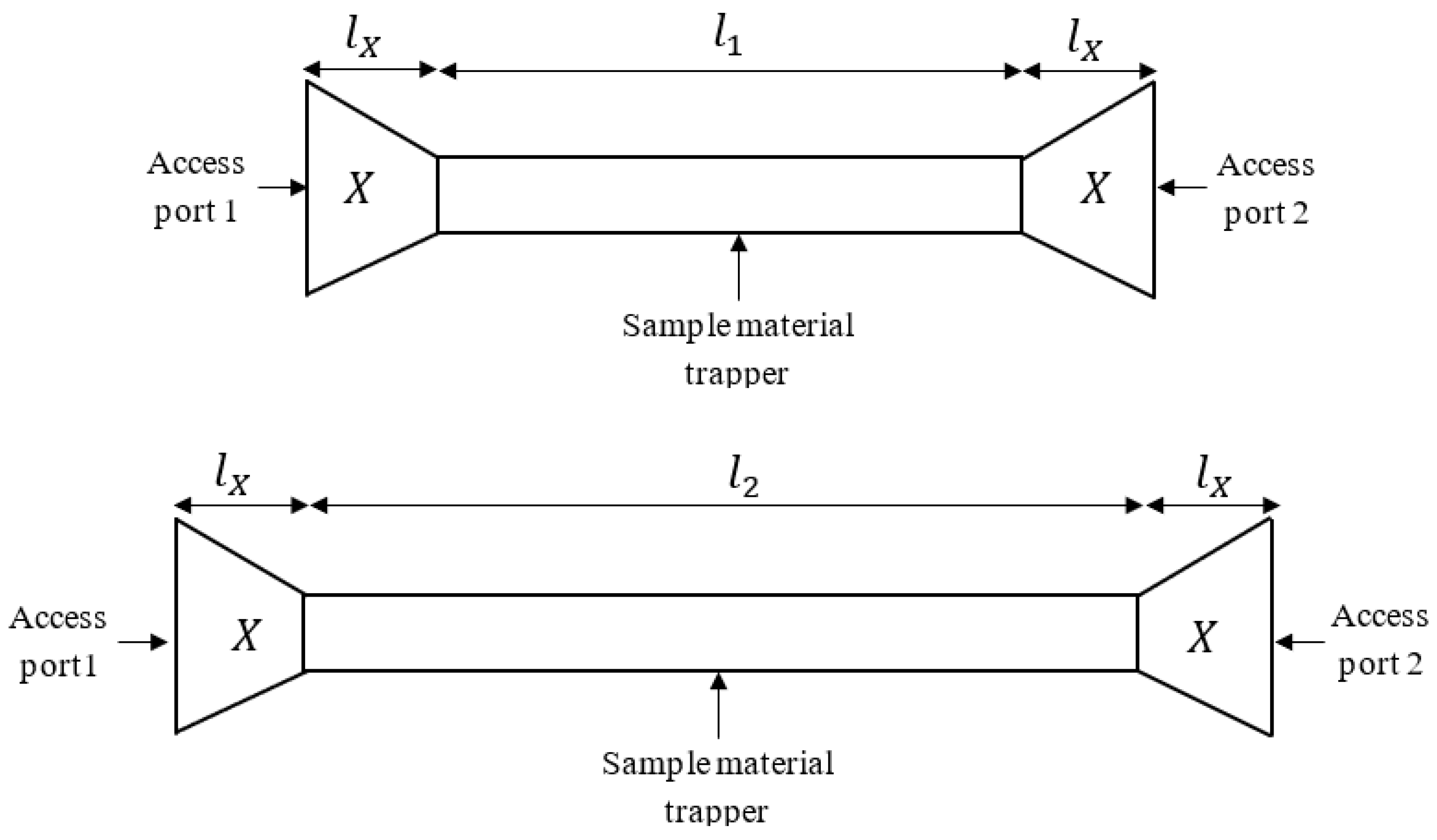
2.1. Topology of the Test Cell
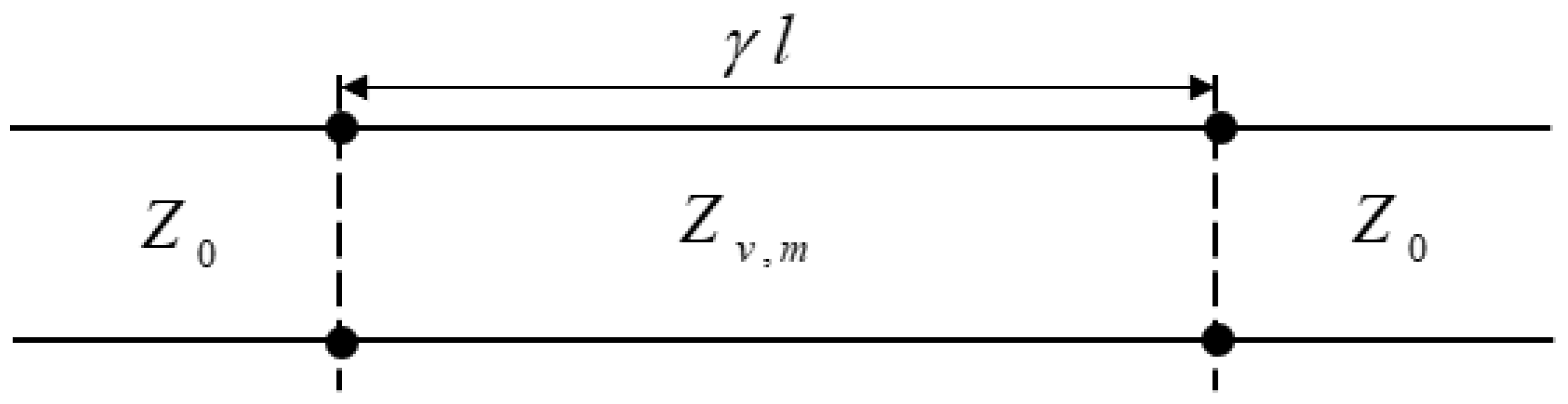
2.2. Mathematical Modeling: Methodology
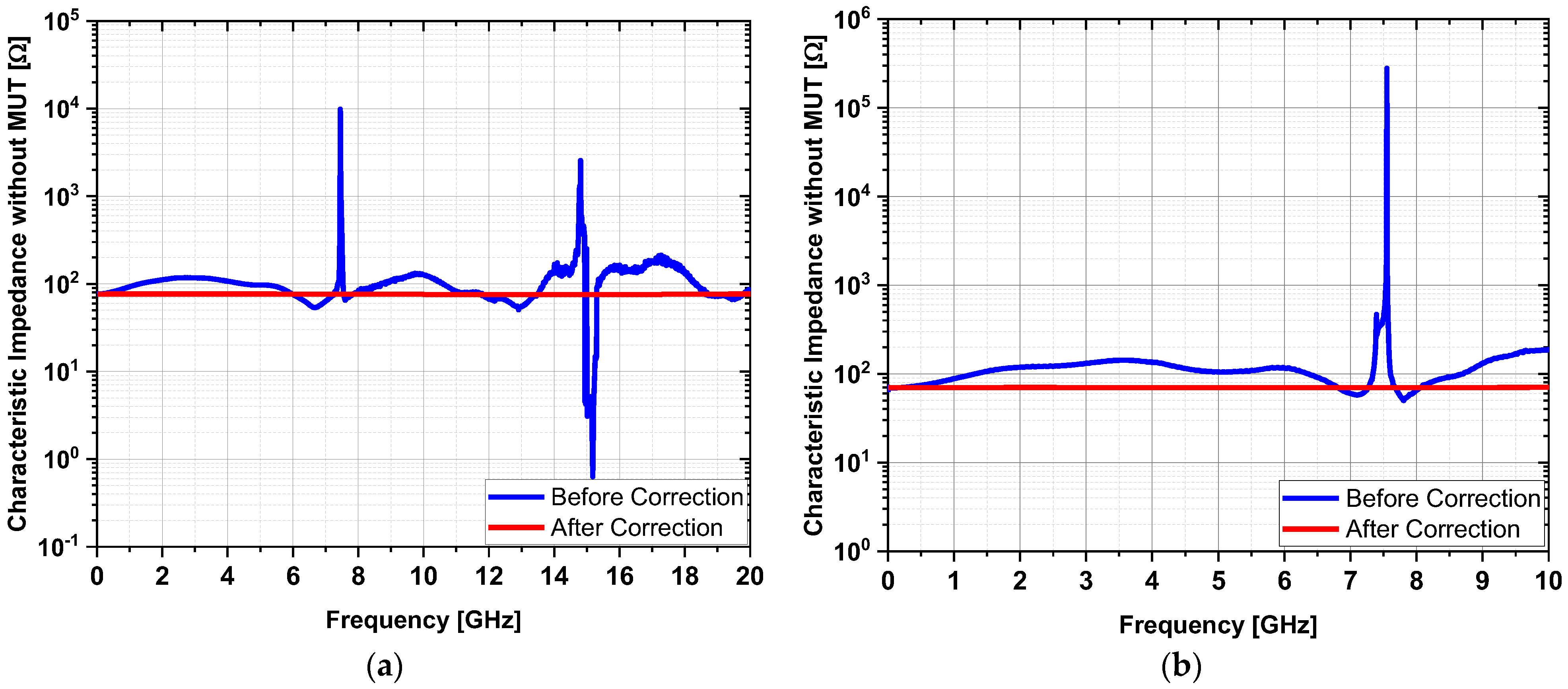
3. Measurement Validations, Results, and Discussion
4. Conclusions
Author Contributions
Funding
Data Availability Statement
Acknowledgments
Conflicts of Interest
References
- Sergei, A.; Wang, X.; Tretyakov, S.A. Fast and Robust Characterization of Lossy Dielectric Slabs Using Rectangular Waveguides. IEEE Trans. Microw. Theory Technol. 2022, 70, 2341–2350. [Google Scholar] [CrossRef]
- Aydinalp, C.; Joof, S.; Dilman, I.; Akduman, I.; Yilmaz, T. Characterization of Open-Ended Coaxial Probe Sensing Depth with Respect to Aperture Size for Dielectric Property Measurement of Heterogeneous Tissues. Sensors 2022, 22, 760. [Google Scholar] [CrossRef] [PubMed]
- Wang, C.; Liu, X.; Gan, L.; Cai, Q. A Dual-Band Non-destructive Dielectric Measurement Sensor Based on Complementary Split-Ring Resonator. Front. Phys. 2021, 9, 669707. [Google Scholar] [CrossRef]
- Severo, S.L.S.; De Salles, Á.A.A.; Nervis, B.; Zanini, B.K. Non-Resonant Permittivity Measurement Methods. J. Microwaves Optoelectron. Electromagn. Appl. 2017, 16, 297–311. [Google Scholar] [CrossRef] [Green Version]
- Sawant, S.S.; Yao, Z.; Jambunathan, R.; Nonaka, A. Characterization of Transmission Lines in Microelectronics Circuits using the ARTEMIS Solver. J. Comput. Phys. 2022. [Google Scholar] [CrossRef]
- Kellermeier, M.; Lemery, F.; Floettmann, K.; Hillert, W.; Aßmann, R. Self-Calibration Technique for Characterization of Integrated THz Waveguides. Phys. Rev. Accel. Beams 2021, 24, 122001. [Google Scholar] [CrossRef]
- Riaz, M.; Kanwal, N. An Improved Parallel Plate Capacitor Apparatus for the Estimation of Dielectric Constants of Solid Materials. Eur. J. Phys. 2019, 40, 025502. [Google Scholar] [CrossRef]
- Phillips, J.; Roman, A. Understanding Dielectrics: Impact of External Salt Water Bath. Materials 2019, 12, 2033. [Google Scholar] [CrossRef] [Green Version]
- Maleki, M.; Mohseni Armaki, S.H.; Hamidi, E. Study of Ferrite Material Characterization using Transmission Line Model. Microw. Opt. Technol. Lett. 2018, 60, 2876–2880. [Google Scholar] [CrossRef]
- Szulim, P.; Gontarz, S. Extraction of Magnetic Field Features to Determine the Degree of Material Strain. Materials 2021, 14, 1576. [Google Scholar] [CrossRef]
- Cho, K.; Jo, S.; Noh, Y.-H.; Lee, N.; Kim, S.; Yook, J.-G. Complex Permittivity Measurements of Steel Fiber-Reinforced Cementitious Composites Using a Free-Space Reflection Method with a Focused Beam Lens Horn Antenna. Sensors 2021, 21, 7789. [Google Scholar] [CrossRef] [PubMed]
- Gonçalves, F.J.F.; Pinto, A.G.M.; Mesquita, R.C.; Silva, E.J.; Brancaccio, A. Free-Space Materials Characterization by Reflection and Transmission Measurements Using Frequency-by-Frequency and Multi-Frequency Algorithms. Electronics 2018, 7, 260. [Google Scholar] [CrossRef] [Green Version]
- Mazaheri, Z.; Koral, C.; Andreone, A. Accurate THz Ellipsometry using Calibration in Time Domain. Sci. Rep. 2022, 12, 7342. [Google Scholar] [CrossRef] [PubMed]
- Vohra, N.; El-shenawee, M. K- and W- Band Free-Space Characterizations of Highly Conductive Radar Absorbing Materials. IEEE Trans. Instrum. Meas. 2021, 70, 8001910. [Google Scholar] [CrossRef]
- Xing, L.; Zhu, J.; Xu, Q.; Zhao, Y.; Song, C.; Huang, Y. Generalised Probe Method to Measure the Liquid Complex Permittivity. IET Microw. Antennas Propag. 2020, 14, 707–711. [Google Scholar] [CrossRef]
- Bowler, N. Four-Point Potential Drop Measurements for Materials Characterization. Meas. Sci. Technol. 2010, 22, 012001. [Google Scholar] [CrossRef]
- Wu, M.; Yao, X.; Zhang, L. An Improved Coaxial Probe Technique for Measuring Microwave Permittivity of Thin Dielectric Materials. Meas. Sci. Technol. 2000, 11, 1617–1622. [Google Scholar] [CrossRef]
- Wang, X.; Guo, H.; Zhou, C.; Bai, J. High-resolution probe design for measuring the dielectric properties of human tissues. Biomed. Eng. Online 2021, 20, 86. [Google Scholar] [CrossRef]
- Williams, D.F.; Marks, R.B. Accurate Transmission Line Characterization. IEEE Microw. Guid. Wave Lett. 1993, 3, 247–249. [Google Scholar] [CrossRef]
- Pérez-Escribano, M.; Márquez-segura, E. Parameters Characterization of Dielectric Materials Samples in Microwave and Millimeter-Wave Bands. IEEE Trans. Microw. Theory Technol. 2021, 69, 1723–1732. [Google Scholar] [CrossRef]
- Huber, O.; Faseth, T.; Magerl, G.; Arthaber, H. Dielectric Characterization of RF-Printed Circuit Board Materials by Microstrip Transmission Lines and Conductor-Backed Coplanar Waveguides Up to 110 GHz. IEEE Trans. Microw. Theory Technol. 2018, 66, 237–244. [Google Scholar] [CrossRef]
- Steiner, C.; Walter, S.; Malashchuk, V.; Hagen, G.; Kogut, I.; Fritze, H.; Moos, R. Determination of the Dielectric Properties of Storage Materials for Exhaust Gas Aftertreatment Using the Microwave Cavity Perturbation Method. Sensors 2020, 20, 6024. [Google Scholar] [CrossRef] [PubMed]
- Kumar, A.; Sharma, S. Measurement of Dielectric and Loss Factor of the Dielectric Material at Microwave Frequencies. Prog. Electromagn. Res. 2007, 69, 47–54. [Google Scholar] [CrossRef] [Green Version]
- Kombolias, M.; Obrzut, J.; Postek, M.T.; Poster, D.L.; Obeng, Y.S. Method Development for Contactless Resonant Cavity Dielectric Spectroscopic Studies of Cellulosic Paper. Anal. Lett. 2020, 53, 424–435. [Google Scholar] [CrossRef]
- Saf, O.; Erol, H.; Erkin, A. A Method for Material Characterization of Sealing System Elastomers using Sound Transmission Loss Measurements. Polym. Test. 2022, 111, 107618. [Google Scholar] [CrossRef]
- Bartley, P.G.; Begley, S.B. A New Free-Space Calibration Technique for Materials Measurement. In Proceedings of the 2012 IEEE International Instrumentation and Measurement Technology Conference Proceedings, Graz, Austria, 13–16 May 2012; pp. 1–5. [Google Scholar] [CrossRef]
- Yong, S.; Khilkevich, V.; Liu, Y.; Gao, H.; Hinaga, S.; De, S.; Padilla, D.; Yanagawa, D.; Drewniak, J. Dielectric Loss Tangent Extraction Using Modal Measurements and 2-D Cross-Sectional Analysis for Multilayer PCBs. IEEE Trans. Electromagn. Compat. 2020, 62, 1278–1292. [Google Scholar] [CrossRef]
- Noel, H.; Lovera, M.; Luis, J.; Cervantes, O.J.-L.; Perez-Ramos, A.-E.; Corona-Chavez, A.; Saavedra, C.E. Microstrip Sensor and Methodology for the Determination of Complex Anisotropic Permittivity using Perturbation Techniques. Sci. Rep. 2022, 12, 2205. [Google Scholar] [CrossRef]
- Pozar, D.M. Microwave Engineering, 4th ed.; Wiley: Hoboken, NJ, USA, 2012; ISBN 978-0-470-63155-3. [Google Scholar]
- M’Pemba, J.E.D.; Bouesse, G.F.; Moukanda Mbango, F.; M’Passi-Mabiala, B. Probes in Transmission with Material Variable Thicknesses to Extract the Material Complex Relative Permittivity in 1.7–3 GHz. Meas. Sens. 2022, 20–21, 100369. [Google Scholar] [CrossRef]
- Lountala, M.G.; Moukanda Mbango, F.; Ndagijimana, F.; Lilonga-Boyenga, D. Movable short-circuit technique to extract the relative permittivity of materials from a coaxial cell. J. Meas. Eng. 2019, 7, 183–194. [Google Scholar] [CrossRef]
- Moukanda Mbango, F.; M’Pemba, J.E.D.; Ndagijimana, F.; M’Passi-Mabiala, B. Use of Two Open-Terminated Coaxial Transmission-Lines Technique to Extract the Material Relative Intrinsic Parameters. IEEE Access 2020, 8, 138682–138689. [Google Scholar] [CrossRef]
- Orend, K.; Baer, C.; Musch, T. A Compact Measurement Setup for Material Characterization in W-Band Based on Dielectric Waveguides. Sensors 2022, 22, 5972. [Google Scholar] [CrossRef] [PubMed]
- Al Takach, A.; Moukanda Mbango, F.; Ndagijimana, F.; Al-Husseini, M.; Jomaah, J. Two-Line Technique for Dielectric Material Characterization With Application in 3D-Printing Filament Electrical Parameters Extraction. Prog. Electromagn. Res. M 2019, 85, 195–207. [Google Scholar] [CrossRef] [Green Version]
- Reynoso-Hernández, J.A. Unified Method for Determining the Complex Propagation Constant of Reflecting and Nonreflecting Transmission Lines. IEEE Microw. Wirel. Components Lett. 2003, 13, 351–353. [Google Scholar] [CrossRef]
- Ghione, G.; Pirola, M. Microwave Electronics: Measurement and Materials Characterization; John Wiley & Sons: Hoboken, NJ, USA, 2017; ISBN 9781316756171. [Google Scholar]
- Costa, F.; Borgese, M.; Degiorgi, M.; Monorchio, A. Electromagnetic Characterisation of Materials by Using Transmission/Reflection (T/R) Devices. Electronics 2017, 6, 95. [Google Scholar] [CrossRef] [Green Version]
- Farcich, N.J.; Salonen, J.; Asbeck, P.M. Single-Length Method Used to Determine the Dielectric Constant of Polydimethylsiloxane. IEEE Trans. Microw. Theory Technol. 2008, 56, 2963–2971. [Google Scholar] [CrossRef]
- Lu, Z.; Lanagan, M.; Manias, E.; MacDonald, D.D. Two-Port Transmission line Technique for Dielectric Property Characterization of Polymer Electrolyte Membranes. J. Phys. Chem. B 2009, 113, 13551–13559. [Google Scholar] [CrossRef] [PubMed]
- Sun, J.; Lucyszyn, S. Extracting Complex Dielectric Properties from Reflection-Transmission Mode Spectroscopy. IEEE Access 2018, 6, 8302–8321. [Google Scholar] [CrossRef]
- Wadell, B.C. Transmission Line Design Handbook; Artech House: Norwood, MA, USA, 1991; ISBN 0-96006-436-9. [Google Scholar]
- Hasar, U.C.; Kaya, Y.; Ozturk, G.; Ertugrul, M. Propagation Constant Measurements of Reflection-Asymmetric and Nonreciprocal Microwave Networks From S-Parameters Without Using a Reflective Standard. Measurement 2020, 165, 108126. [Google Scholar] [CrossRef]
- Papio Toda, A.; De Flaviis, F. 60-GHz Substrate Materials Characterization Using the Covered Transmission-Line Method. IEEE Trans. Microw. Theory Technol. 2015, 63, 1063–1075. [Google Scholar] [CrossRef]
- Caspers, F. RF engineering basic concepts: S-parameters. arXiv 2012, arXiv:1201.2346. [Google Scholar]
- Moukanda Mbango, F.; Al Takach, A.; Ndagijimana, F. Complex Relative Permittivity Extraction Technique of Biotechnology Materials in Microwaves Domain. Int. J. Electron. Commun. Instrum. Eng. Res. Dev. 2019, 9, 33–42. [Google Scholar] [CrossRef]
- Moukanda Mbango, F.; Lountala, M.G.; MPemba, E.J.D.; Ndagijimana, F.; Lilonga-Boyenga, D.; MPassi-Mabiala, B. Comparison of Materials Characterization Methods Using One-Port and Two-Port Transmission Line Principles. Int. J. Eng. Appl. 2021, 9, 370–381. [Google Scholar] [CrossRef]
- Moukanda Mbango, F. Contribution à la Caractérisation Electrique des Matériaux Utilisés en Microélectronique RadioFréquence. Ph.D. Thesis, Université Joseph-Fourier, Saint-Martin-d’Hères, France, 2008. [Google Scholar]


| Aquarium Sand | Semi-Flex 100% | PLA 100% | Semolina | Polenta | Q-Cell 5020 | |
|---|---|---|---|---|---|---|
| Fixture shape | Circular | Rectangular | Rectangular | Circular | Circular | Circular |
| Medium | 3.093 | 2.449 | 2.485 | 2.388 | 1.892 | 1.238 |
| –Coefficient | 1.172 | 0.9 | 1.128 | 1.019 | 0.848 | 0.502 |
| –Coefficient | 1.07 | 1.117 | 0.85 | 0.793 | 1.036 | 1.45 |
| Scanned bandwidth frequency (GHz) | 10 | 10 | 10 | 13.5 | 10 | 20 |
| Eigenvalue Principle | New Suggested Approach | |||
|---|---|---|---|---|
| Aquarium Sand | 3.082 | 1.067 × 10⁻⁴ | 3.093 | 0.01 |
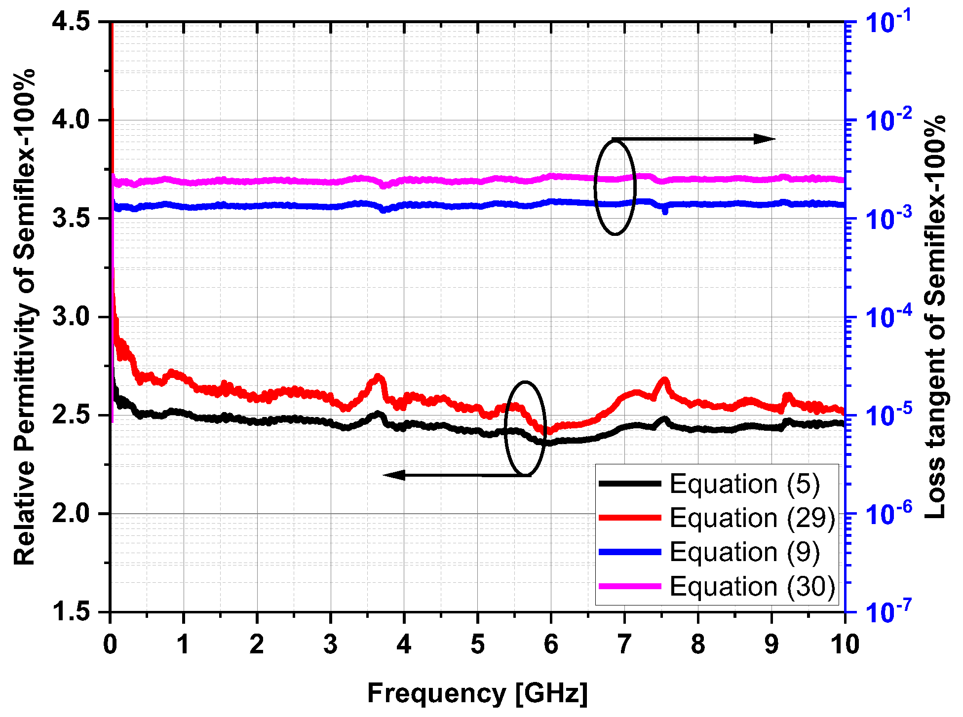
| Semi-Flex 100% | 2.584 | 9.689 × 10⁻⁴ | 2.449 | 0.022 |
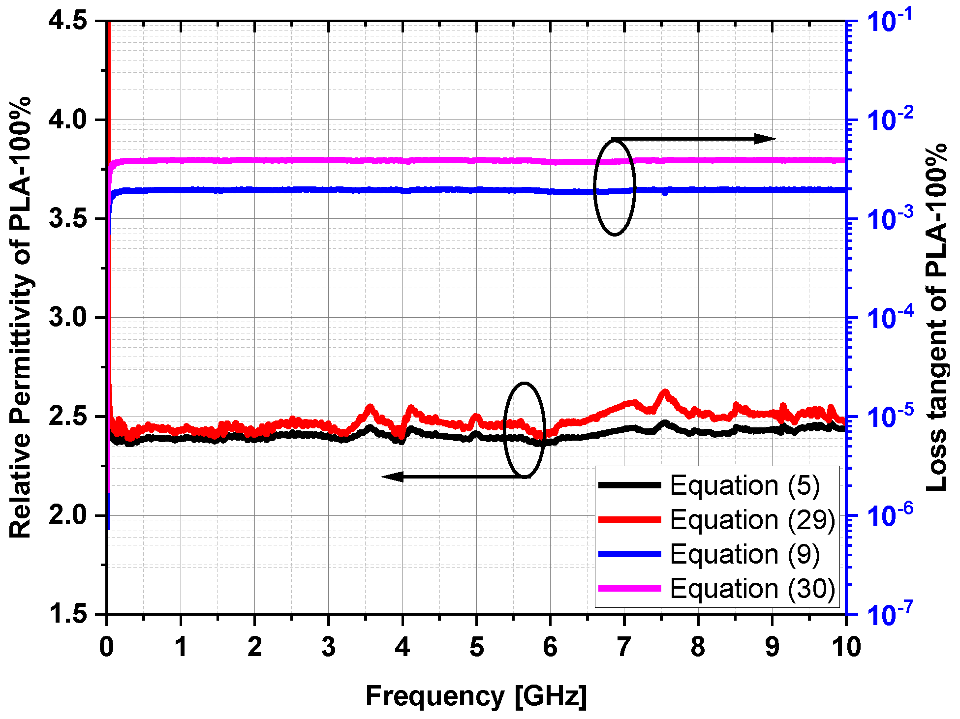
| PLA 100% | 2.469 | 5.49 × 10⁻³ | 2.485 | 0.022 |
| Semolina | 2.376 | 3.347 × 10⁻³ | 2.388 | 6.187 × 10⁻³ |
| Polenta | 1.928 | 4.298 × 10⁻³ | 1.892 | 2.861 × 10⁻³ |
| Q-Cell 5020 | 1.164 | 7.979 × 10⁻⁴ | 1.238 | 0.018 |
| Equation (7) | Equation (36) | |
|---|---|---|
| Aquarium Sand | 0.01 | 1.067 × 10⁻⁴ |
| Semi-Flex 100% | 0.022 | 9.689 × 10⁻⁴ |
| PLA 100% | 0.022 | 5.49 × 10⁻³ |
| Semolina | 6.187 × 10⁻³ | 3.347 × 10⁻³ |
| Polenta | 2.861 × 10⁻³ | 4.298 × 10⁻³ |
| Q-Cell 5020 | 0.018 | 4.14 × 10⁻⁴ |
Publisher’s Note: MDPI stays neutral with regard to jurisdictional claims in published maps and institutional affiliations. |
© 2022 by the authors. Licensee MDPI, Basel, Switzerland. This article is an open access article distributed under the terms and conditions of the Creative Commons Attribution (CC BY) license (https://creativecommons.org/licenses/by/4.0/).
Share and Cite
Moukanda Mbango, F.; Bouesse, G.F.; Ndagijimana, F. Extraction of the Complex Relative Permittivity from the Characteristic Impedance of Transmission Line by Resolving Discontinuities. Electronics 2022, 11, 4035. https://doi.org/10.3390/electronics11234035
Moukanda Mbango F, Bouesse GF, Ndagijimana F. Extraction of the Complex Relative Permittivity from the Characteristic Impedance of Transmission Line by Resolving Discontinuities. Electronics. 2022; 11(23):4035. https://doi.org/10.3390/electronics11234035
Chicago/Turabian StyleMoukanda Mbango, Franck, Ghislain Fraidy Bouesse, and Fabien Ndagijimana. 2022. "Extraction of the Complex Relative Permittivity from the Characteristic Impedance of Transmission Line by Resolving Discontinuities" Electronics 11, no. 23: 4035. https://doi.org/10.3390/electronics11234035