
Flight Delay Prediction Model Based on Lightweight Network ECA-MobileNetV3


Tianjin Key Laboratory of Advanced Signal Processing, Civil Aviation University of China, Tianjin 300300, China
*
Author to whom correspondence should be addressed.
Electronics 2023, 12(6), 1434; https://doi.org/10.3390/electronics12061434
Submission received: 15 February 2023
/
Revised: 14 March 2023
/
Accepted: 16 March 2023
/
Published: 17 March 2023
(This article belongs to the Special Issue Advances in Intelligent Data Analysis and Its Applications)
Abstract
:In exploring the flight delay problem, traditional deep learning algorithms suffer from low accuracy and extreme computational complexity; therefore, the deep flight delay prediction algorithm is difficult to directly deploy to the mobile terminal. In this paper, a flight delay prediction model based on the lightweight network ECA-MobileNetV3 algorithm is proposed. The algorithm first preprocesses the data with real flight information and weather information. Then, in order to increase the accuracy of the model without increasing the computational complexity too much, feature extraction is performed using the lightweight ECA-MobileNetV3 algorithm with the addition of the Efficient Channel Attention mechanism. Finally, the flight delay classification prediction level is output via a Softmax classifier. In the experiments of single airport and airport cluster datasets, the optimal accuracy of the ECA-MobileNetV3 algorithm is 98.97% and 96.81%, the number of parameters is 0.33 million and 0.55 million, and the computational volume is 32.80 million and 60.44 million, respectively, which are better than the performance of the MobileNetV3 algorithm under the same conditions. The improved model can achieve a better balance between accuracy and computational complexity, which is more conducive mobility.
1. Introduction
In recent years, China’s air traffic industry has grown rapidly with the implementation of the 13th Five-Year Plan for Civil Aviation [1]. However, the number of flights continues to grow, but the normal rate of flights is becoming lower and lower. During this period, the Civil Aviation Administration carried out total control of flight slots and adjusted flight structure, and the problem of flight delays was alleviated. According to a report from the Civil Aviation Work Conference 2022 held by the Civil Aviation Administration of China [2], since 2020, due to the impact of the epidemic, the number of flights has significantly decreased abnormally, so flight delays during the epidemic are not considered. In addition, China will overtake the United States as the largest air transport organization in 2029, according to research from the International Air Transport Association (IATA) [3]. With the COVID-19 epidemic under effective control, the volume of air traffic will also increase rapidly. Therefore, the speed of air traffic recovery and the projections of international reports firmly reflect the urgent traffic demand of China’s air traffic industry. Serious flight delays are likely to trigger “mass incidents of air passengers” [4,5,6], thus endangering the public safety of the airport and the personal safety of the passengers. Understanding flight delays in advance has become a pressing issue for civil aviation. To this end, a large number of studies have been carried out by domestic and foreign scholars in related fields.
The traditional flight delay prediction methods mainly include statistical inference, simulation and modeling, and machine learning methods [7]. Xu et al. [8] proposed a permutation and incremental permutation SVM algorithm considering the demand of flight volume and real-time refreshment of flight data and validated it on manual data. Finally, the accuracy of flight delay prediction can reach more than 80%. Similarly, Luo ‘s team [9] and Luo ‘s team [10] also gradually considered using support vector machines or improved support vectors to analyze flight delays. In view of the irregular dynamic distribution attributes of flight data, Cheng et al. [11] proposed a classification prediction model of flight delay based on C4.5 decision tree to avoid the impact of flight distribution changes on the algorithm model, which is a certain improvement compared with the traditional Bayesian algorithm. Nigam and Govinda [12] analyzed the flight data and meteorological data of several airports in the United States and used the logistic regression algorithm in the machine learning algorithm to predict the flight departure delay. Khanmohammadi et al. [13] proposed a flight delay prediction model based on an improved Artificial Neural Network (ANN), and they used multiple linear N-1 coding to preprocess complex airport data models. Wu et al. [14] proposed a flight delay spread prediction model based on CBAM-CondenseNet, which enhances the transmission of deep information in the network structure by adopting a channel and spatial attention mechanism to increase the prediction accuracy. When using deep learning to predict flight delay, these scholars chose a relatively deep learning network, which requires a lot of computing time and resources. They can only choose to deploy the flight delay algorithm to the PC terminal. However, for the deployment requirements of mobile terminals, there is no trade-off between the accuracy and computational complexity of the prediction algorithm.
Recently, experts from home and abroad have carried out in-depth research and innovation in lightweight materials. In the beginning, experts used knowledge distillation, model pruning and other methods to try out algorithms. The former first trains a Net-T network and then uses network distillation to obtain a smaller Net-S network, thus achieving the effect of a simplified model. The latter simplified the model through channel pruning and other operations on the trained model [15,16,17,18,19]. Lightweight convolutional neural networks are an emerging branch of deep learning algorithms. This type of network applies lightweight operations to the algorithm itself and continuously innovates the algorithm from within so that it can maximize accuracy and continuously meet the computational power requirements of mobile devices. For example, the peerless team [20] proposed the ShuffleNet series algorithm, which uses the Channel Shuffle and Channel split operations [21] to speed up network and feature reuse, and the lightweight neural network Efficientnet algorithms presented by the Google team [22]. This algorithm comprehensively considers the input data size, network depth, and width, and proposes a model compound scaling method to control model computing power and ensure accuracy. Iandola et al. [23] proposed a lightweight SqueezeNet algorithm that proposes a Fire module structure to design the network structure. In this structure, to extract features and lessen model computation, single-layer and double-layer convolutions were used. The Google team [24] proposed MobileNet series algorithms, which are extremely influential in lightweight neural networks, which use deep separable convolution and SE attention mechanism for feature extraction and combine with structures, such as inverted residual error, which considerably improve the accuracy and computational performance of the model [25,26]. Excellent results have been achieved in face recognition, image classification, target detection, etc. [27,28,29].
To sum up, in view of the problems of low prediction accuracy and high computational complexity of the existing flight delay prediction algorithms, which are not conducive to deployment on mobile devices and other devices, this paper proposes an improved lightweight ECA-MobilenetV3 algorithm, which replaces the SE model with a lightweight ECA (Efficient Channel Attention) module, effectively reducing the computational complexity of the model without losing accuracy; it lays a foundation for the application of the model in mobile devices. The experiment uses real domestic meteorological data and flight data for analysis and verification.
The organizational structure of this paper is as follows: Section 1 introduces the background and significance of the paper, as well as the research status at home and abroad. Section 2 proposes and introduces the ECA-MobileNetV3 network model. Section 3 introduces the building process of a flight delay prediction model in detail. Section 4 shows the analysis of the experimental results and the application of the model. Section 5 summarizes the work of this paper and describes the future work.
2. Design of the ECA-MobileNetV3 Network Model
2.1. The Overall Structure of the Network
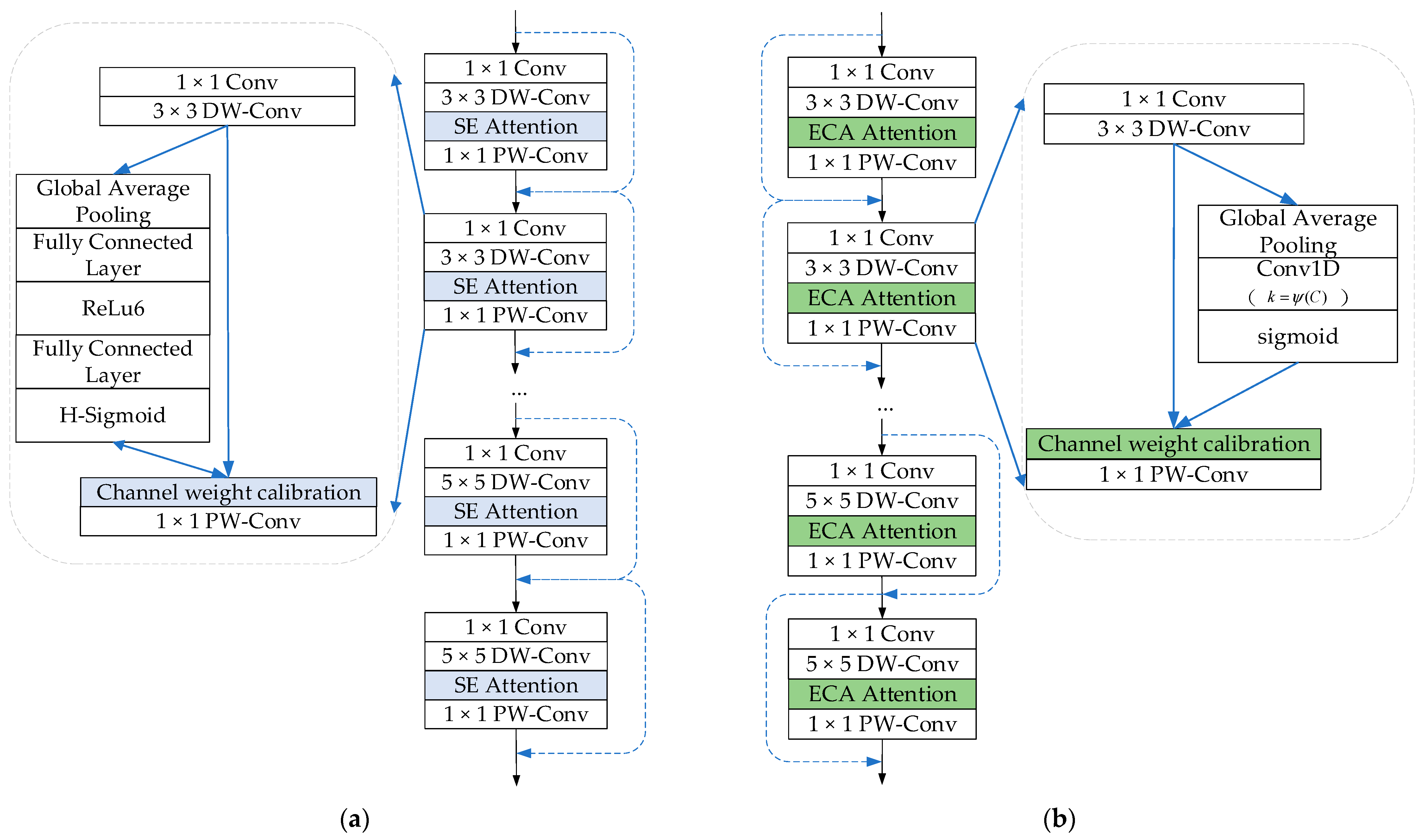
The network structure of the MobileNetV3 algorithm is shown in Figure 1a. Inheriting the three advantages of deep separable convolution, inverted residue structure, and linear bottleneck structure of MobileNetV2 network, the algorithm adds the SE attention mechanism in each inverted residue model [30]. In this paper, considering the non-lightweight nature of the SE attention mechanism, we propose an improved lightweight ECA-MobileNetV3 network, which replaces the SE module with the lightweight ECA attention mechanism [31], and the improved algorithm structure is shown in Figure 1b. The ECA-MobileNetV3 algorithm uses 1-dimensional convolution and cross-channel interaction methods to obtain channel importance, which effectively reduces the computational complexity of the model while ensuring the accuracy of the model.
The ECA-MobileNetV3 algorithm uses a deep convolution kernel of a different size for the inverted residual structure. As can be seen from the structural configuration table for the ECA-MobileNetV3 algorithm listed in Table 1, the size of the deep convolution kernel in the inverted residual module 1, module 2, and module 3 is , while the size of the deep convolution kernel in the remaining inverted residual module is . Width Multiplier is the hyper parameter in the MobileNetV3 network; by adjusting its size, one can change the channel number of the output matrix in each layer of the whole network, so as to quickly change the model size; the number of output feature matrix channels is . The α denotes the channel factor, which is the hyper parameter in the MobileNetV3 network. By adjusting its size, the number of channels in the output matrix in each layer of the network can be changed, so that the model size can be changed quickly.
2.2. Lightweight ECA Module
There is an SE module in the MobileNetV3 algorithm, in which the feature matrix is first dimensioned down and then dimensioned up to obtain the weight channel importance. However, the dimensionality reducing operation between the two completely connected layers is not conducive to the weight learning of the channel and will lose certain feature information. Moreover, the model’s calculation load will increase a little with the fully connected layer. Therefore, this paper considers using the lightweight attention mechanism ECA module to replace the SE attention mechanism module in MobileNetV3. The ECA module also functions as a channel attention mechanism, completing the acquisition of channel weights through an adaptive one-dimensional convolution and a cross-channel interaction technique without dimensionality reduction. The model can effectively reduce the computational complexity while maintaining the property.
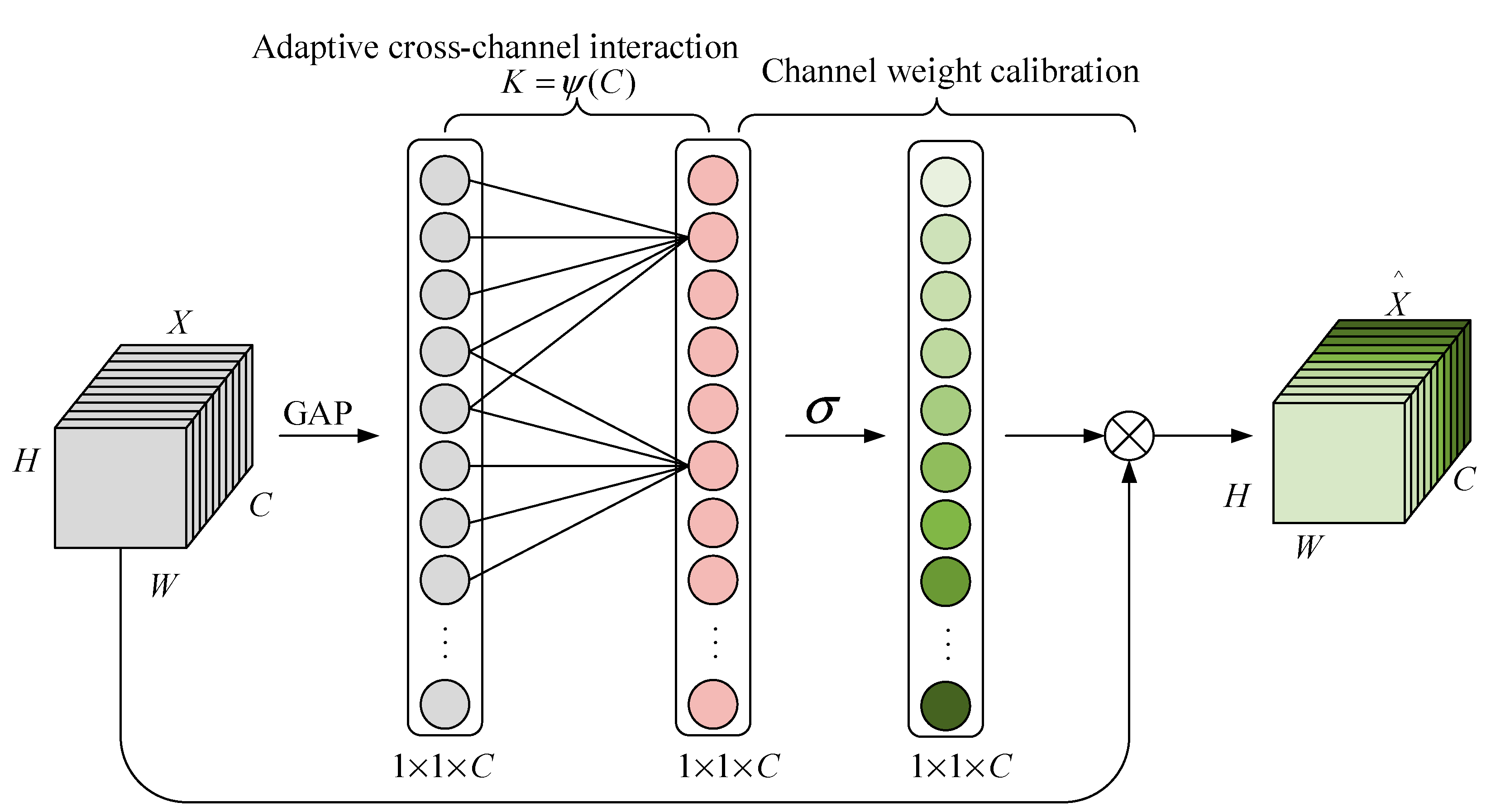
Figure 2 depicts the ECA module’s general structure. Assuming that the feature matrix before the input to the ECA attention mechanism is , through global average pooling, the features first reduce the width and height of the feature matrix. The model then enters the adaptive one-dimensional convolution calculation to complete the acquisition of feature weights, as shown in Formula (1), in which adaptation refers to the adaptive selection of k adjacent channels in the process of obtaining channel weights, as shown in Formula (2).
In Formula (1), represents the channel-acquired weights, the Sigmoid activation function, the adaptive one-dimensional convolution, and the feature matrix after global average pooling. In Formula (2), k represents the number of local cross-channel interactions, which is the size of the one-dimensional convolutional kernel, represents the number of channels in the feature matrix, and and b represent constants. The experiment is set to 2 and 1, respectively, according to the requirements of the original paper.
2.3. Network Training of Forward Propagation
An inverted residue module inside ECA-MobileNetV3 consists of traditional convolution, / deep convolution, ECA attention mechanism, and point-by-point convolution. Each layer is convolved with a BN regularization layer and an activation function layer. The ECA-MobileNetV3 algorithm has 11 reverse residual modules. In the first three reverse residual modules, the ReLU function is chosen as the activation function for the first conventional convolutional layer and the second depth layer, as shown in Formula (3), and the H-Swish function as the activation function, as shown in Formula (4); all successive convolutional layers use the linear function as an activation function and Sigmoid function for channel weight, as shown in Formula (5).
Through the above description, we can obtain the feature matrix in the calculation process, the convolution layer can be expressed as the following Formulas (6) and (7), which can derive a residual module after three convolution operations, and they can be represented by Formulas (8)–(10).
where represents the weight of the -th feature to the -th feature in the layer , represents the bias of the -th feature in the layer , represents the output value before the -th feature in layer passes the activation function, represents the activation function, and represents the mapping value of the -th feature in the layer after the activation function.
In addition, the feature matrix enters the ECA module after entering the deconvolutional module and passing through traditional convolutional layers and deep convolutional layers. The ECA module lies between deep convolution and pointwise convolution. As a complete calculation unit for acquiring channel weights, its forward propagation process is shown in Formula (11):
where represents the feature matrix after the deep convolution operation, and the second half of the formula represents the feature weights acquired through the ECA module.
2.4. Network Training of Back Propagation
After the forward propagation of the ECA-MobileNetV3 algorithm is completed to obtain the predicted value of the model, the loss function between it and the true value is computed. Then, the chain derivative rule is used to obtain the chain derivative of the error term of the training samples, and the weight parameters and the bias are updated continuously until the network model converges. Chain derivative rule can also be called BP (back propagation) [32]. The error term between layers and is calculated according to the rule, as shown in Formula (12). The chain analysis results of weight and bias within a residual module are shown in Formulas (13) and (14):
where represents the loss function, represents the error value of the -th eigenvalue in layer , represents the weight of neurons from -th to -th feature in layer , and represents the multiplication between matrices., , and , respectively, represent the error terms between traditional convolutional layer, deep convolutional layer, ECA module, and point-by-point convolutional layer. According to Formulas (13) and (14), the weight and bias can be updated from back to forward, respectively.
3. Flight Delay Prediction Model Based on ECA-MobileNetV3
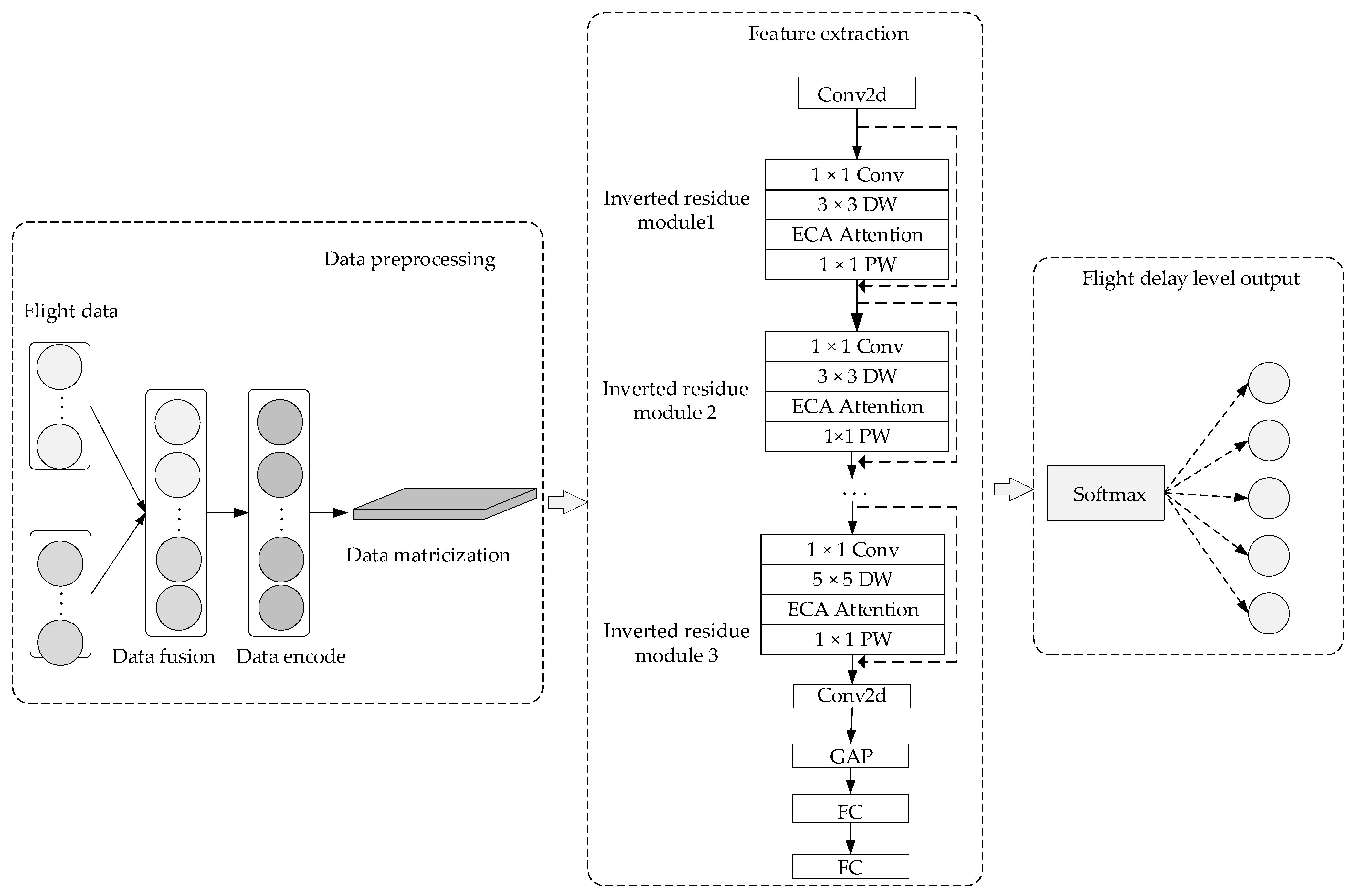
The overall structure of the flight delay prediction model based on ECA-MobileNetV3 is shown in Figure 3. The flight delay prediction model is divided into three parts [33]: data processing, feature extraction of the delay prediction model, and classification prediction of the model.
3.1. Data Preprocessing
The dataset used in this paper is mainly the flight dataset integrated with meteorological information and independently built. The data acquisition mainly comes from two sources: the flight dataset from March 2018 to March 2019 provided by the East China Air Traffic Administration and the meteorological dataset observed by the Automatic Weather Observation System (AWOS) [34], and the flight dataset from September 2019 to October 2020 provided by the North China Air Traffic Administration and the corresponding meteorological dataset. The flight dataset integrated with meteorological information contains multiple characteristic variables, including flight number, departure airport, destination airport, departure time, arrival time, delay time, flight status, etc. It also includes meteorological data, such as temperature, humidity, wind speed, precipitation, etc. According to the different sources of data acquisition, the dataset is divided into the Shanghai Hongqiao Airport dataset provided by the East China Air Traffic Control Bureau and the Beijing–Tianjin–Hebei Airport Cluster dataset provided by the North China Air Traffic Control Bureau. The Shanghai Hongqiao Airport dataset contains 301,594 sample data, and the Beijing–Tianjin–Hebei Airport Cluster dataset contains 1,048,576 sample data. The dataset also contains missing values and duplicate values, the flight data provided by the air traffic control bureau is manually recorded, and the meteorological data are collected by the airport’s sensor equipment. There will be errors and omissions in the manually recorded data, and some data will be missing and incomplete due to sensor failure. During data integration processing, the same data may also be recorded repeatedly, so the dataset needs to be cleaned and processed to ensure data quality.
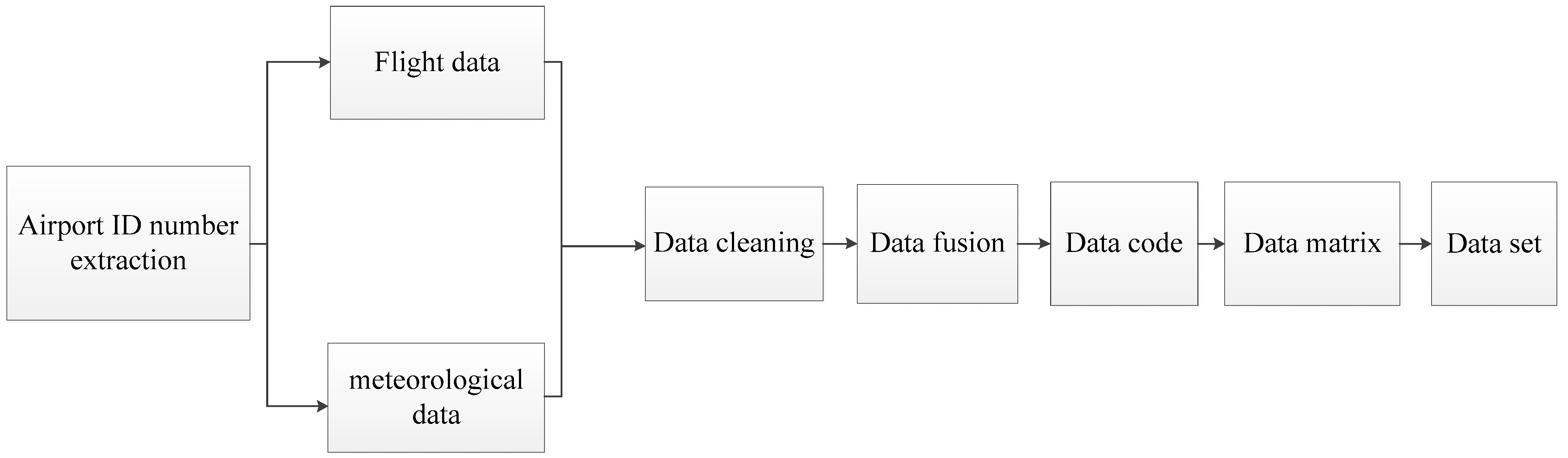
A series of preprocessing operations is performed on the dataset before feeding into the lightweight convolutional neural network algorithm. Figure 4 shows a data preprocessing flowchart. The whole process can be divided into: data cleaning, data fusion, data encoding, and matrix quadrature. For the dataset of Shanghai Hongqiao Airport, the flights of Shanghai Hongqiao Airport should be extracted from the original dataset according to the planned departure airport and planned arrival airport according to the four-character code of civil aviation airport “ZSSS” (Shanghai Hongqiao International Airport). Similarly, for the Beijing–Tianjin–Hebei airport cluster dataset, flights from major airports in Beijing, Tianjin, and Shijiazhuang were, respectively, extracted according to the four-character code of civil aviation airport “ZBAA” (Beijing Capital International Airport), “ZBAD” (Beijing Daxing International Airport), “ZBTJ” (Tianjin Binhai International Airport), and “ZBSJ” (Shijiazhuang Zhengding International Airport), and then the subsequent data pretreatment work was carried out.
The first step in data preprocessing is data cleaning: attribute columns with many nulls in the dataset, duplicate data and attribute deletion, and other operations. The second step is data fusion operation: set the time attribute in the meteorological data as the association primary key I, set the planned start time and planned landing time in the flight data as the association primary key II according to the airport ID, and then conduct the association fusion between the primary key I and the primary key II. In order to enhance the data, the 10 min meteorological information is fused in this paper to enlarge the feature information of the fused data. The third step is the data encoding operation: Considering that the categorical data in the dataset contain low-base data and high-base data, as well as the numerical attributes of the data, the mixed encoding methods of Min–Max coding [35] and CatBoost coding [36] are adopted in this paper to encode the dataset, so as to ensure that the data remain in the same dimensional range before input into the algorithm. There is also no dimensional explosion. The fourth step is the data matrix operation: since the MobileNetV3 algorithm belongs to the convolutional neural network, its input data is required to be in the form of a matrix, so the dataset in this paper needs to be converted from the form of vector to the form of matrix before input into the algorithm, so as to meet the input requirements.
3.2. Feature Extraction of the Delay Prediction Model
The processed dataset needs to be transformed into tensor form and fed into the model for feature extraction and training. The specific feature extraction process is as follows: After the ECA-MobileNetV3 network model accepts the input characteristic matrix, the characteristic matrix first passes through the first standard convolution layer, which converts the input characteristic matrix into a set of characteristic graphs and then activates it immediately following a nonlinear activation function. Next, these feature maps will pass through multiple inverse residual modules composed of a standard convolution layer, deep convolution layer, ECA attention mechanism module, and point-by-point convolution layer and activation function. These convolution layers with deep separability can effectively reduce the model parameters and calculation amount, and multiple inverse residual models can extract features at different levels. During this period, the ECA-MobileNetV3 network uses an ECA module and feature fusion technology to fuse feature maps at different levels to improve the expression ability of feature maps. Then, the feature map passes through a global average pooling layer. The global average pooling layer can reduce the dimension of the feature map into a vector. Finally, this vector maps the feature vector to the target category through a fully connected layer classifier to complete the classification task.
3.3. Classification Prediction
The pre-processed dataset needs to be transformed into tensor form and fed into the model for training. According to the relevant definition of flight delay in Normal Flight Management Regulations [37] issued by the Civil Aviation Administration of China in 2017, on this basis, this paper subdivides the delay situation into five different time periods. In this paper, the five levels of flight delay are taken as the labels of the dataset, and the flight arrival delay time is taken as the flight delay time T. It defines the difference between the actual arrival time and the planned arrival time.
According to the classification of flight delay levels given in Table 2 and the sample number of each delay level in the two datasets, when T is less than 15 min, it is considered as delay-free; that is, the flight delay level is 0 and the label is 0. When T is between 15 and 60 min, it is considered to be slightly delayed; that is, the flight delay level is 1 and the label is 1. When T is between 60 and 120 min, it is considered moderate delay; that is, the flight delay level is 2 and the label is 2. When T is between 120 and 240 min, it is considered to be highly delayed; that is, the flight delay level is 3 and the label is 3. When T is above 240 min, it is considered a severe delay, that is, a flight delay level of 4 with a label of 4.
The flight delay prediction algorithm then uses the Softmax classifier to determine the flight delay level. Softmax function is a commonly used activation function, which is often used for the final output of multi-classification problems. The original Softmax classifier formula is shown in (15), where represents the -th sample, represents the number of categories, and represents the number of categories. The Softmax function can map a q-dimension vector to a q-dimension probability distribution, where the value of each element represents the probability size of the category. Therefore, the classifier can compute a probability value for each delay level, and the highest value is used as each datum’s final result. The Softmax classifier formula is shown in (16):
Among them, is the final output of the flight delay prediction model, is the optimal parameter obtained by the model, represents the serial number of data quantity, and represents the classification number of flight delay level.
4. Interpretation
4.1. Experimental Environment and Model Parameter Configuration
The computer used in this paper was set up as follows under the described experimental setting: the processor was an Intel Xeon E5-1620 with a CPU frequency of 3.60 GHz; memory 16.004 GB; the OS is Ubuntu16.04. The graphics accelerator GeForce GTX TITAN Xp; the deep learning development framework is Tensorflow 2.3.0. The sample size of the Shanghai Hongqiao Airport dataset used in the experiment is 301,089, the feature attribute quantity is 64, and the size after matrix is ; the sample size of Beijing–Tianjin–Hebei airport cluster dataset is 1,650,797, the feature attribute quantity is 72, and the size after matrix is . The specific experimental parameter configurations used to train the model are shown in Table 3 below.
4.2. Evaluation Index of the Model
Loss value and accuracy rate are evaluation metrics that characterize how well a deep learning algorithm fits. The loss value is mainly used to measure the difference between the predicted result of the model and the actual value and can be calculated from the loss function, which is negatively correlated with accuracy, with higher accuracy leading to smaller loss values. The percentage of samples that produced accurate predictions compared to all samples is known as the accuracy rate. The formula is shown in (17), where represents the predicted correct sample.
Computational complexity can describe the hardware consumption at runtime. The higher the complexity, the more memory is occupied and the higher the processing time required. It is mainly divided into spatial complexity and time complexity: spatial complexity is expressed in terms of the number of parameters. The number of parameters of single-layer convolutional layer and single-layer fully connected layer in the algorithm can be approximated as Formulas (18) and (19). The time complexity is expressed in computational quantities, which might be understood as the quantity of FLOPs (Floating Point Operations). The computation amount of single-layer convolutional layer and single-layer fully connected layer can be approximated as Formulas (20) and (21).
In Formulas (18) and (19), and are the number of parameters of single-layer convolutional layer and single-layer fully connected layer, respectively, is the convolutional kernel size in the current layer, is the number of input feature channels of the current layer, is the number of output feature channels of the current layer, and is the input feature size of the current layer. In Formulas (20) and (21), and are the calculated amount of single-layer convolutional layer and single-layer full connection layer, respectively. Thus, 1 represents the output feature size of the full connection layer, and the other parameters have the same meaning in the parameter number formula.
4.3. Loss Values and Accuracy Rates
The validation will be performed on the Shanghai Hongqiao Airport dataset and the Beijing–Tianjin–Hebei Airport dataset.
Based on the Shanghai Hongqiao Airport dataset, the accuracy and the magnitude of loss values in the MobileNetV3 algorithm and ECA-MobileNetV3 algorithm with different channel factors are given in Table 4. According to Table 4, from the longitudinal analysis, the accuracy of MobileNetV3 and ECA-MobileNetV3 algorithms gradually increases and the loss value gradually decreases as the channel factor becomes larger, and the accuracy of the MobileNetV3 algorithm reaches the highest at 98.87% when the channel factor is 1.00. The ECA-MobileNetV3 algorithm achieves the highest accuracy of 98.97% at a channel factor of 0.75. From a cross-sectional perspective, the accuracy of the ECA-MobileNetV3 algorithm with the addition of the ECA attention mechanism module is higher than that of the original MobileNetV3 algorithm for the same number of channel factors, and it can be seen that the improved algorithm does not lose accuracy on a single-airport dataset such as the Shanghai Hongqiao Airport dataset.
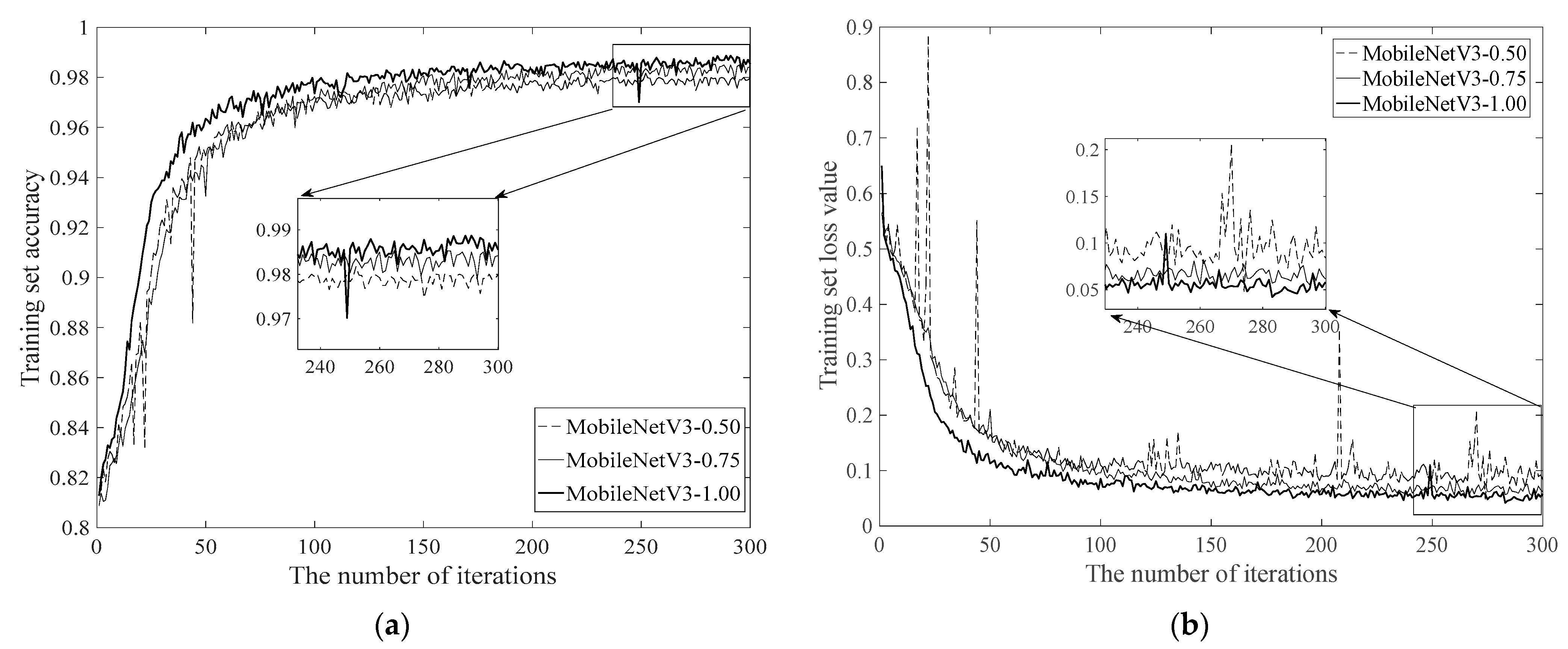
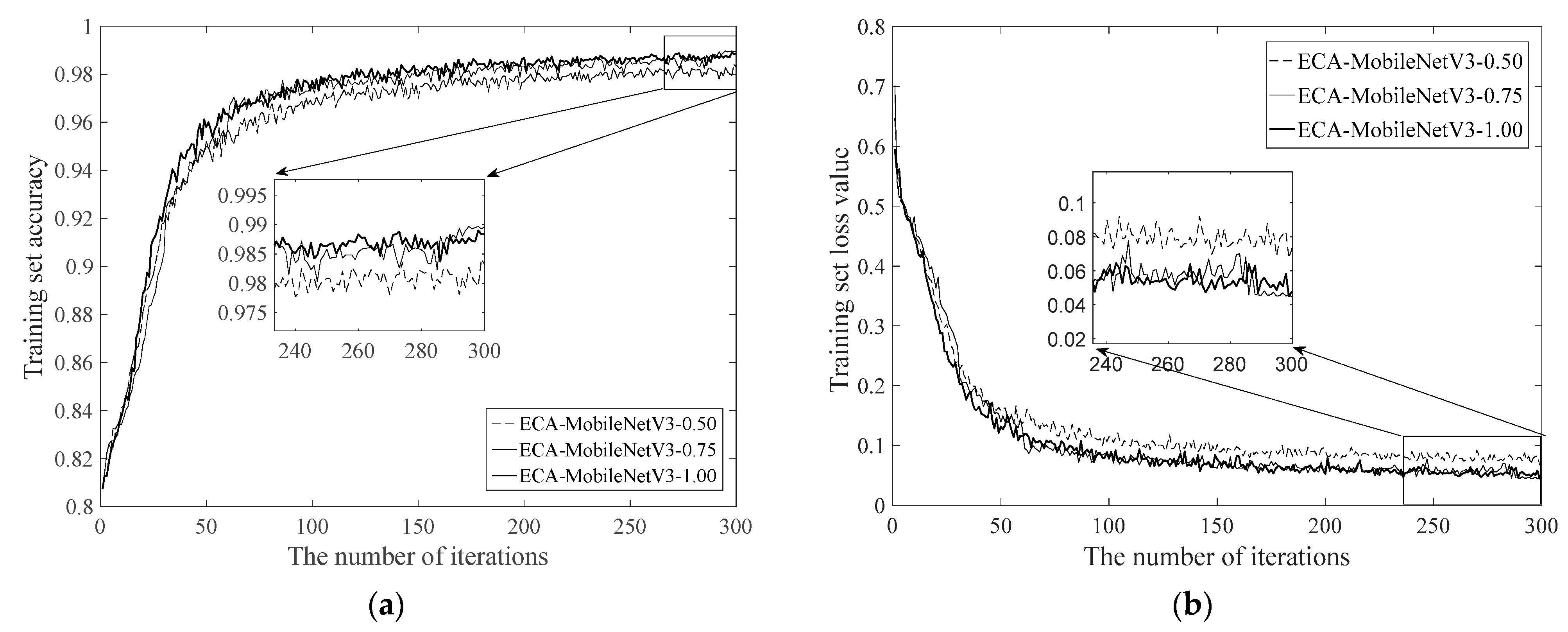
Based on the dataset of Shanghai Hongqiao Airport, the accuracy and loss curves of the MobileNetV3 algorithm and ECA-MobileNetV3 algorithm under different channel factors are, respectively, presented in Figure 5 and Figure 6. According to the trend of the curves, at different channel factors, the accuracy rate gently increases while the loss value gently decreases. The loss values and accuracies of MobileNetV3 and ECA-MobileNetV3 tend to stabilize when the number of training rounds is around 300. From the experimental results, the MobileNetV3 algorithm has a loss value of about 0.0419 when the channel factor is 1.00. The highest accuracy was 98.87%. When the channel factor is 0.75, the lowest loss value of the ECA-MobileNetV3 algorithm is about 0.0449, and the highest accuracy is 98.90%. Compared with the MobileNetV3 algorithm, the accuracy of the ECA-MobileNetV3 algorithm with attention mechanism is slightly improved and the loss value is slightly increased.
Based on the Beijing–Tianjin–Hebei airport cluster dataset, according to Table 5, from the longitudinal analysis, as the channel factor becomes larger, the accuracy of the two algorithms gradually increases and the loss value gradually decreases. Further, the accuracy rates of the MobileNetV3 algorithm and ECA-MobileNetV3 algorithm reach the highest when the channel factor is 1.00, and the accuracy rate of the MobileNetV3 algorithm reaches 96.60%; the accuracy rate of the ECA-MobileNetV3 algorithm reaches 96.81%. From a cross-sectional perspective, the accuracy of the ECA-MobileNetV3 algorithm is slightly lower than that of the MobileNetV3 algorithm at channel factor numbers of 0.50 and 0.75, and the accuracy of the improved algorithm is 0.18% lower than that before the improvement at a channel factor of 0.50. At a channel factor of 1.00, the accuracy of the ECA-MobileNetV3 algorithm is slightly higher than that of the MobileNetV3 algorithm, and the accuracy of the improved algorithm is 0.21% higher than that before the improvement. Therefore, on the whole, the improved ECA-MobileNetV3 algorithm has a minor loss in accuracy and still has some advantages in a multi-airport-associated cluster dataset such as the Beijing–Tianjin–Hebei airport cluster dataset.
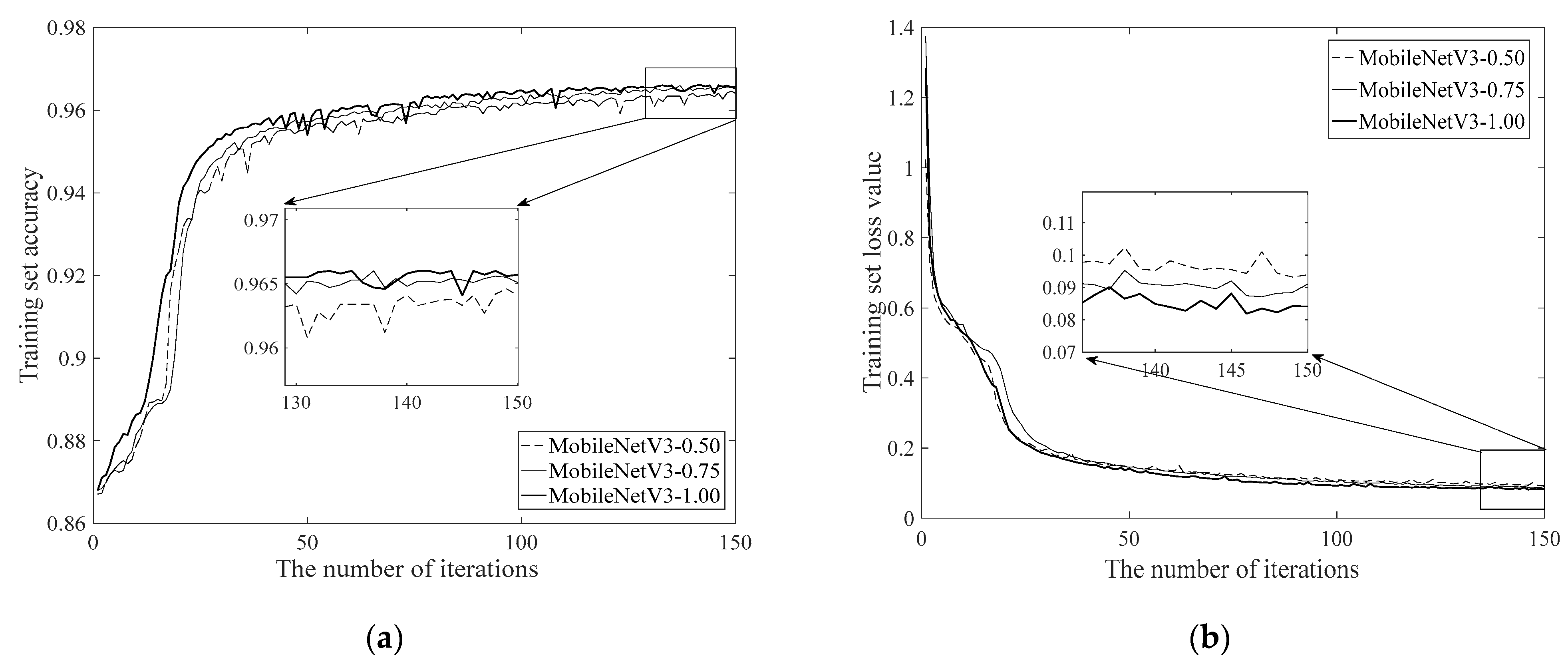
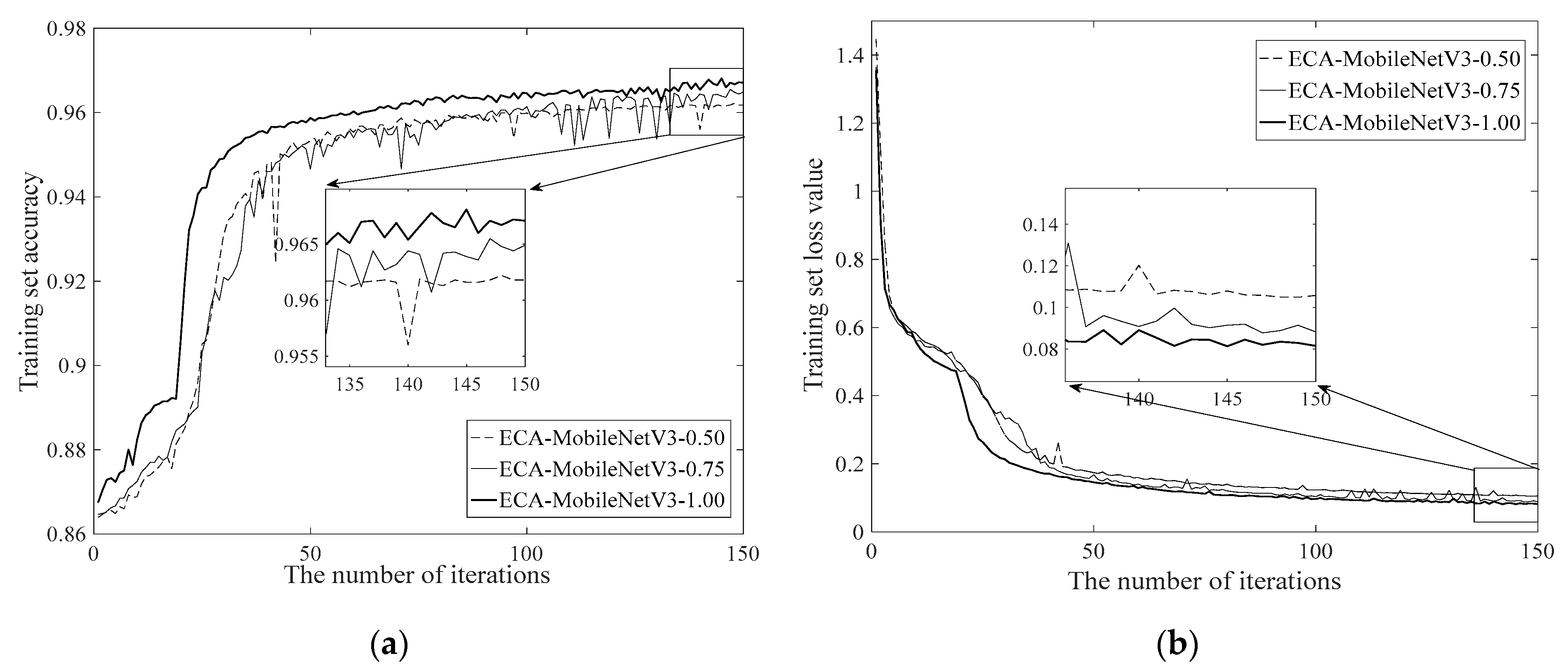
Based on the Beijing–Tianjin–Hebei airport cluster dataset, the accuracy and loss curves of the MobileNetV3 algorithm and ECA-MobileNetV3 algorithm under different channel factors are, respectively, presented in Figure 7 and Figure 8. According to the trend of the curves, at different channel factors, the accuracy rate gently increases while the loss value gently decreases. The loss values and accuracies of MobileNetV3 and ECA-MobileNetV3 tend to stabilize when the number of training rounds is around 150. From the experimental results, the MobileNetV3 algorithm has a loss value of about 0.0819 when the channel factor is 1.00. The highest accuracy was 96.60%. When the channel factor is 1.00, the lowest loss value of the ECA-MobileNetV3 algorithm is about 0.0813, and the highest accuracy is 96.81%. Compared with the MobileNetV3 algorithm, the accuracy of the ECA-MobileNetV3 algorithm with an attention mechanism is slightly improved, while the loss value is slightly decreased.
4.4. Complex Calculation of the Model
Validation will be performed on the Shanghai Hongqiao Airport dataset and the Beijing–Tianjin–Hebei Airport dataset.
Based on the Shanghai Hongqiao Airport dataset, Table 6 displays the suggested algorithm’s accuracy and computational complexity before and after the enhancement. Vertically, as the channel factor increases, the MobileNetV3 algorithm’s accuracy rises together with the model’s complexity. The model complexity and accuracy of the ECA-MobileNetV3 algorithm increase with the channel factor. However, for channel factors of 0.75 and 1.0, the accuracy rate does not improve significantly due to the complexity of the model but gradually stabilizes. From a horizontal perspective, under the same channel factor, the ECA-MobileNetV3 model can efficiently minimize the number of parameters and computation without sacrificing accuracy.
Based on the Beijing–Tianjin–Hebei airport cluster dataset, the computational complexity and accuracy of the proposed algorithm before and after the improvement are shown in Table 7. From the longitudinal point of view, as the channel factor increases, the complexity of the MobileNetV3 model increases and the accuracy improves. However, with channel factors of 0.75 and 1.00, the accuracy increases slightly and remains essentially stable. As the channel factor increases, the complexity of the ECA-MobileNetV3 model increases and the accuracy improves. When the channel factors are 0.75 and 1.0, the accuracy is significantly improved. From a horizontal perspective, the computational complexity of the ECA-MobileNetV3 model is effectively reduced with little loss in accuracy for the same channel factor.
It is clear from the experimental findings on the aforementioned two datasets that the computational cost and precision of the proposed model are not only linear. We can find algorithms that better balance the accuracy and computational complexity of the model, which is also the direction of efforts in lightweight neural networks. By computing conditions on different mobile devices, it is possible to match flight delay prediction models of different sizes to maximize the model utilization.
4.5. Comparison of Different Network Models
Compared with traditional deep learning algorithms, the modified ECA-MobileNetV3 achieves better performance in terms of computational complexity and model accuracy when dealing with real domestic flight datasets with weather information fusion. In this regard, this paper verifies the single airport and airport group datasets, compares the ECA-MobileNetV3_1.00 model with the traditional ResNet [38], DenseNet [39] algorithm, and MobileNetV2 algorithm under the same channel factor and analyzes it from the following three aspects. ResNet and DenseNet are models that have been trained and widely used in large-scale datasets and have achieved good results in many computer vision and natural language processing tasks. Therefore, they are very representative models and can be used as benchmarks for other models. MobileNetV2, as the leader in the lightweight model, has been widely used in many mobile device applications. MobileNetV2 is the predecessor of MobileNetV3, which can verify whether the improvement in ECA-MobileNetV3 is effective. Taking MobileNetV2 as a comparative test can also provide reference and inspiration for more lightweight model design. The results are shown in Table 8.
In the Hongqiao Airport dataset, the accuracy of the ECA-MobileNetV3_1.00 algorithm increases by 3.34% and 3.96% and the number of citations decreases by 10.63 million and 6.49 million, respectively, compared to the other two traditional networks. The calculated amounts were reduced by 1375.64 million and 444.6 million, respectively. In the single airport dataset, it can be seen that the enhanced ECA-MobileNetV3 model outperforms in terms of accuracy and computational complexity. In addition, when compared to the MobileNetV2 method at the same channel factor, the accuracy of the enhanced algorithm is decreased by 0.16%, and the number of parameters and computational cost are decreased, respectively, by 171 million and 16.99 million. As compared to the MobileNetV2 algorithm at the same level, it can be seen that the upgraded algorithm achieves a better balance between model complexity and accuracy.
In the Beijing–Tianjin–Hebei airport cluster dataset, the accuracy of the ECA-MobileNetV3_1.00 model increases by 2.48% and 3.05% and the reference number decreases by 10.63 million and 6.49 million, respectively, compared to the other two traditional networks. The calculated amounts were reduced by 1547.63 million and 520.10 million, respectively. On the airport cluster dataset, it can be shown that the revised model performs quite well in the three evaluation measures mentioned above. Additionally, the ECA-MobileNetV3 algorithm’s accuracy is increased by 0.82% when compared to MobileNetV2 at the same channel factor, while the algorithm’s computational cost and parameter count are decreased by 1.71 million and 27.96 million, respectively. As is evident, the improved model also achieves a better balance of the above three metrics compared to the MobileNetV2 algorithm of the same level.
4.6. Application of the Model
At present, the flight delay prediction Web visualization system based on the flight delay prediction model of ECA-MobileNetV3 has been put into use in the air traffic control bureau. The system uses the flight delay prediction model studied in this paper to predict flight delay and then displays the predicted delay results on the web page through the Web visualization technology and can carry out statistical analysis on the historical delay information, so as to explore the deeper laws of delay generation, for example, to see in which time periods of the day and in which months of the year flight delays mainly occur. This application mainly takes advantage of the high prediction accuracy of the flight delay prediction model studied in this paper. The subsequent application direction will focus on the advantages of light weight. The lightweight model has the characteristics of fast prediction speed, less demand for computing resources, higher real-time performance, and portability. Therefore, this model can be deployed on some low-power devices, such as mobile devices and sensors. This can quickly process data input and quickly update forecast results and provide real-time information for airlines and the base to help them plan and manage flight missions.
5. Conclusions
This paper studies the lightweight neural network MobileNetV3 algorithm and the improved ECA-MobileNetV3 algorithm. By using the Shanghai Hongqiao Airport dataset and the Beijing–Tianjin–Hebei Airport Cluster dataset, for example, analysis and practical application of the model, the following conclusions are drawn: The algorithm proposed in this paper can effectively reduce the computational complexity in the model without loss of accuracy or with a small loss of accuracy by replacing the SE module in the original MobileNetV3 algorithm with a lightweight ECA attention mechanism module. Compared with the ResNet algorithm, DenseNet algorithm, and MobileNetV2 algorithm under the same channel factor, the improved ECA-MobileNetV3 algorithm has more advantages in computational complexity and accuracy. The flight delay prediction model based on ECA-the MobileNetV3 algorithm has the advantage of light weight compared with the flight delay prediction model that has been deployed now. The lightweight flight delay model can bring faster execution speed, fewer computing resources, higher real-time performance, and higher flexibility and portability, which can greatly lay the foundation for subsequent deployment on mobile terminals and other platform devices, and for airlines, the airport and passengers provide better service and better experience. However, there is still a lot of room for improvement in the process of research in this paper. On the one hand, the number of flight samples with different delay levels is quite different, which will affect the accuracy of flight prediction. It is necessary to consider the impact of sample imbalance on model training. On the other hand, the problem of flight delay is time-varying, and the prediction model needs to be updated at any time. The next step is to explore how to achieve a real-time update of the model and improve the practicability of the model.
Author Contributions
Methodology, J.Q.; validation, B.C. and C.L.; investigation, J.Q.; writing—original draft preparation, B.C., C.L. and J.W.; writing—review and editing, B.C. All authors have read and agreed to the published version of the manuscript.
Funding
This research was funded by the Tianjin Municipal Education Commission Scientific Research Program, grant number 2022ZD006, and the Fundamental Research Funds for the Central Universities, grant number 3122019185.
Data Availability Statement
Not applicable.
Conflicts of Interest
The authors declare no conflict of interest.
References
- Five Major Development Tasks Clearly Clarified by the 13th Five-Year Plan for Civil Aviation. Available online: http://caacnews.com.cn/1/1/201612/t20161222_1207217.html (accessed on 22 December 2016).
- Report on the 2022 National Civil Aviation Work Conference. Available online: http://www.caac.gov.cn/XWZX/MHYW/202201/t20220110_210827.html (accessed on 10 January 2022).
- IATA: The Global Air Passenger Volume Will Reach 8.2 Billion Person-Times in 2007. Available online: https://www.ccaonline.cn/news/top/461390.html (accessed on 30 October 2018).
- Zhang, Y. Study on Group Time Countermeasures caused by Abnormal Flights-Take CEA as An Example. Master’s Thesis, East China University of Political Science and Law, Shanghai, China, 2018. [Google Scholar]
- Zhang, M. Research on Optimization of Countermeasures for Handling Mass Incidents of Passengers caused by Flight Delays. Master’s Thesis, Handong University of Finance and Economics, Jinan, China, 2016. [Google Scholar]
- Li, X.; Liu, G.C.; Yan, M.C.; Zhang, W. Economic losses of airlines and passengers caused by flight delays. Syst. Eng. 2007, 25, 20–23. [Google Scholar]
- Liu, B.; Ye, B.J.; Tian, Y. Overview of flight delay prediction methods. Aviat. Comput. Technol. 2019, 49, 124–128. [Google Scholar]
- Xu, T.; Ding, J.L.; Gu, B.; Wang, J.D. Airport flight delay warning based on the incremental arrangement of support vector machines. Aviat. J. 2009, 30, 1256–1263. [Google Scholar]
- Luo, Q.; Zhang, Y.H.; Cheng, H.; Li, C. Model of hub airport flight delay based on aviation information network. Syst. Eng. Theory Pract. 2014, 34, 143–150. [Google Scholar]
- Luo, Z.S.; Chen, Z.J.; Tang, J.H.; Zhu, Y.W. A flight delay prediction study using SVM regression. Transp. Syst. Eng. Inf. 2015, 15, 143–149, 172. [Google Scholar]
- Cheng, H.; Li, Y.M.; Luo, Q.; Li, C. Study on Prediction of arrival flight delay based on C4.5 decision tree method. Syst. Eng. Theory Pract. 2014, 34, 239–247. [Google Scholar]
- Nigam, R.; Govinda, K. Cloud Based Flight Delay Prediction using logistic Regression. In Proceedings of the 2017 International Conference on Intelligent Sustainable Systems (ICISS), Palladam, India, 7–8 December 2017. [Google Scholar]
- Khanmohammadi, S.; Tutun, S.; Kucuk, Y. A new multilevel input layer artificial neural network for predicting flight delays at JFK airport. Procedia Comput. Sci. 2016, 95, 237–244. [Google Scholar] [CrossRef] [Green Version]
- Wu, R.B.; Zhao, Y.Q.; Qu, J.Y. Flight delay spread prediction model based on CBAM-CondenseNet. J. Electron. Inf. Technol. 2021, 43, 187–195. [Google Scholar]
- Hition, G.; Vinyals, O.; Dean, J. Distilling the knowledge in a neural network. Comput. Sci. 2015, 14, 38–39. [Google Scholar]
- Vongkulbhisal, J.; Vinayavekhin, P.; Visentini-scarzanella, M. Unifying Heterogeneous Classifiers with Heterogeneous Classifiers with Distillation. In Proceedings of the IEEE/CVF Conference on Computer Vision and Pattern Recognition (CVPR), Long Beach, CA, USA, 15–20 June 2019. [Google Scholar]
- Zhuang, l.; Li, J.G.; Shen, Z.; Zhang, C.M. Learning Efficient Convolutional Networks Through Network Slimming. In Proceedings of the IEEE International Conference on Computer Vision (ICCV), Venice, Italy, 22–29 October 2017. [Google Scholar]
- He, Y.; Zhang, X.; Sun, J. Channel Pruning for Accelerating Very Deep Neural Networks. In Proceedings of the IEEE International Conference on Computer Vision (ICCV), Venice, Italy, 22–29 October 2017. [Google Scholar]
- Luo, J.H.; Wu, J.X.; Lin, W.Y. Thinet: A Filter Level Pruning Method for Deep Neural Network Compression. In Proceedings of the IEEE International Conference on Computer Vision (ICCV), Venice, Italy, 22–29 October 2017. [Google Scholar]
- Zhang, X.; Zhou, X.; Lin, M. ShuffleNet: An Extremely Efficient Convolutional Neural Network for Mobile Devices. In Proceedings of the IEEE Conference on Computer Vision and Pattern Recognition (CVPR), Salt Lake City, UT, USA, 18–23 June 2018. [Google Scholar]
- Ma, N.N.; Zhang, X.Y.; Zheng, H.T. ShuffleNetV2: Practical Guidelines for Efficient CNN Architecture Design. In Proceedings of the European Conference on Computer Vision (ECCV), Munich, Germany, 8–14 September 2018. [Google Scholar]
- Tan, M.; Le, Q.E. EfficientNet: Rethinking Model Scaling for Convolutional Neural Networks. arXiv 2019, arXiv:1905.11946. [Google Scholar]
- Iandola, F.N.; Han, S.; Moskewicz, M.W. SqueezeNet: AlexNet-level Accuracy with 50x Fewer Parameters and <0.5 MB Model Size. arXiv 2016, arXiv:1602.07360. [Google Scholar]
- Howard, A.G.; Zhu, M.; Chen, B. MobileNets: Efficient Convolutional Neural Networks for Mobile Vision Applications. arXiv 2017, arXiv:1704.04861. [Google Scholar]
- Sandler, M.; Howard, A.; Zhu, M. MobileNetV2: Inverted Residuals and Linearbottlenecks. In Proceedings of the IEEE Conference on Computer Vision and Pattern Recognition (CVPR), Salt Lake City, UT, USA, 18–23 June 2018. [Google Scholar]
- Howard, A.; Sandler, M.; Chu, G. Searching for Mobilenetv3. In Proceedings of the IEEE/CVF International Conference on Computer Vision (ICCV), Seoul, Republic of Korea, 27 October–3 November 2019. [Google Scholar]
- Cai, Q.J.; Peng, C.; Shi, X.W. Based on the MobieNetV2 lightweight face recognition algorithm. Comput. Appl. 2020, 40, 65–68. [Google Scholar]
- Qi, Y.K. Lightweight algorithm for pavement obstacle detection based on MobileNet and YOLOv3. Comput. Syst. Appl. 2022, 31, 176–184. [Google Scholar]
- Hu, J.L.; Shi, Y.P.; Xie, S.Y.; Chen, P. Improved MobileNet face recognition system based on Jetson Nano. Sens. Microsyst. 2021, 40, 102–105. [Google Scholar]
- Hu, J.; Shen, L.; Albanie, S.; Sun, G.; Wu, E. Squeeze-and-Excitation Networks. In Proceedings of the IEEE Conference on Computer Vision and Pattern Recognition (CVPR), Salt Lake City, UT, USA, 18–23 June 2018. [Google Scholar]
- Wang, Q.; Wu, B.; Zhu, P. ECA-Net: Efficient Channel Attention for Deep Convolutional Neural Networks. In Proceedings of the IEEE/CVF Conference on Computer Vision and Pattern Recognition (CVPR), Seattle, WA, USA, 14–19 June 2020. [Google Scholar]
- Rumelhart, D.E.; Hinton, G.E.; Williams, R.J. Learning representations by back-propagating errors. Nature 1986, 323, 533–536. [Google Scholar] [CrossRef]
- Qu, J.; Zhao, T.; Ye, M. Flight delay prediction using deep convolutional neural network based on fusion of meteorological data. Neural Process. Lett. 2020, 52, 1461–1484. [Google Scholar] [CrossRef]
- Quality Controlled Local Climatological Data. Available online: https://www.ncdc.noaa.gov/orders/qclcd/ (accessed on 13 February 2019).
- Cao, L. Research on Flight Delay Prediction and Visualization method based on CliqueNet. Master’s Thesis, Civil Aviation University of China, Tianjin, China, 2020. [Google Scholar]
- Prokhorenkova, L.; Gusev, G.; Vorobev, A. CatBoost: Unbiased Boosting with Categorical Features. Adv. Neural Inf. Process. Syst. 2018, 31, 6638–6648. [Google Scholar]
- Flight Normal Management Regulations. Available online: https://xxgk.mot.gov.cn/2020/jigou/fgs/202006/t20200623_3307796.html (accessed on 24 March 2016).
- He, K.; Zhang, X.; Ren, S. Deep Residual Learning for Image Recognition. In Proceedings of the IEEE Conference on Computer Vision and Pattern Recognition (CVPR), Las Vegas, NV, USA, 26 June–1 July 2016. [Google Scholar]
- Huang, G.; Liu, Z.; Weinberger, K.Q. Densely Connected Convolutional Networks. In Proceedings of the IEEE Conference on Computer Vision and Pattern Recognition (CVPR), Honolulu, HI, USA, 21–26 July 2017. [Google Scholar]
Figure 1.
Comparison of the backbone network structure of the two algorithms before and after the improvement. (a) Backbone network structure of the MobileNetV3. (b) Backbone network structure of the ECA-MobileNetV3.
Figure 1.
Comparison of the backbone network structure of the two algorithms before and after the improvement. (a) Backbone network structure of the MobileNetV3. (b) Backbone network structure of the ECA-MobileNetV3.

Figure 2.
Structural diagram of the ECA attention mechanism.

Figure 3.
Flight delay prediction model based on the ECA-MobileNetV3 algorithm.

Figure 4.
Data processing flowchart.

Figure 5.
Comparison of loss values and accuracy for different-width multipliers based on the MobileNetV3 algorithm on Shanghai Hongqiao Airport dataset. (a) Accuracy comparison of different-width multipliers. (b) Loss value comparison of different-width multipliers.
Figure 5.
Comparison of loss values and accuracy for different-width multipliers based on the MobileNetV3 algorithm on Shanghai Hongqiao Airport dataset. (a) Accuracy comparison of different-width multipliers. (b) Loss value comparison of different-width multipliers.

Figure 6.
Comparison of loss values and accuracy for different-width multipliers based on the ECA-MobileNetV3 algorithm on Shanghai Hongqiao Airport dataset. (a) Accuracy comparison of different-width multipliers. (b) Loss value comparison of different-width multipliers.
Figure 6.
Comparison of loss values and accuracy for different-width multipliers based on the ECA-MobileNetV3 algorithm on Shanghai Hongqiao Airport dataset. (a) Accuracy comparison of different-width multipliers. (b) Loss value comparison of different-width multipliers.

Figure 7.
Comparison of loss values and accuracy for different-width multipliers based on the MobileNetV3 algorithm on Beijing–Tianjin–Hebei airport cluster dataset. (a) Accuracy comparison of different-width multipliers. (b) Loss value comparison of different-width multipliers.
Figure 7.
Comparison of loss values and accuracy for different-width multipliers based on the MobileNetV3 algorithm on Beijing–Tianjin–Hebei airport cluster dataset. (a) Accuracy comparison of different-width multipliers. (b) Loss value comparison of different-width multipliers.

Figure 8.
Comparison of loss values and accuracy for different-width multipliers based on the ECA-MobileNetV3 algorithm on Beijing–Tianjin–Hebei airport cluster dataset. (a) Accuracy comparison of different-width multipliers. (b) Loss value comparison of different-width multipliers.
Figure 8.
Comparison of loss values and accuracy for different-width multipliers based on the ECA-MobileNetV3 algorithm on Beijing–Tianjin–Hebei airport cluster dataset. (a) Accuracy comparison of different-width multipliers. (b) Loss value comparison of different-width multipliers.


Table 1.
Configuration table of the flight delay prediction model based on the ECA-MobileNetV3 algorithm.
Table 1.
Configuration table of the flight delay prediction model based on the ECA-MobileNetV3 algorithm.
| Network Layer | ||||
|---|---|---|---|---|
| Input | / | - | 1 | |
| Traditional convolutional layer | / | [] | 16 | |
| Inverted residuals module 1 | Traditional convolutional layer | / | [] | 16 |
| Deep convolutional layer | [] | |||
| ECA module | - | |||
| Convolutional layer by point | [] | |||
| Inverted residuals module 2 | Traditional convolutional layer | / | [] | 24 |
| Deep convolutional layer | [] | |||
| ECA module | - | |||
| Convolutional layer by point | [] | |||
| …… | ||||
| Inverted residuals module 11 | Traditional convolutional layer | / | [] | 96 |
| Deep convolutional layer | [] | |||
| ECA module | - | |||
| Convolutional layer by point | [] | |||
| Traditional convolutional layer | / | [] | 88 | |
| GAP (Global Average Pooling) | / | - | - | |
| Fully Connected Layer | - | 1280 | ||
| Dropout layer | - | - | ||
| Fully Connected Layer | - | 5 | ||
Table 2.
Flight delay level classification.
| Flight Delay Grade | Flight Delay Time T (minute) | Hongqiao Airport | Beijing–Tianjin–Hebei Airport Cluster |
|---|---|---|---|
| 0 (No delay) | T ≤ 15 | 242,873 | 898,033 |
| 1 (Mild delay) | 15 < T ≤ 60 | 34,388 | 91,362 |
| 2 (Moderate delay) | 60 < T ≤ 120 | 14,904 | 32,053 |
| 3 (Highly delayed) | 120 < T ≤ 240 | 7379 | 16,932 |
| 4 (Heavy delay) | T > 240 | 2049 | 10,195 |
Table 3.
Table of configuration of experimental parameters.
| Parameter Name | Hongqiao Airport Parameters Take the Value | Beijing–Tianjin–Hebei Airport Group Parameter Value |
|---|---|---|
| Iteration number | 300 | 150 |
| Train_test_split | 9:1 | 9:1 |
| Loss function | Cross entropy | Cross entropy |
| Optimizer | Adam | Adam |
| Learning rate | 0.001 | 0.000001 |
| Dropout | 0.2 | 0.2 |
| Training batch volume | 256 | 128 |
| Test batch volume | 256 | 128 |
| Width Multiplier | 0.50/0.75/1.00 | 0.50/0.75/1.00 |
Table 4.
Comparison table of accuracy and loss values for different-width multipliers on Shanghai Hongqiao Airport dataset.
Table 4.
Comparison table of accuracy and loss values for different-width multipliers on Shanghai Hongqiao Airport dataset.
| Width Multiplier | MobileNetV3 | ECA-MobileNetV3 | ||
|---|---|---|---|---|
| Accuracy | Loss Value | Accuracy | Loss Value | |
| 0.50 | 98.00% | 0.0716 | 98.41% | 0.0675 |
| 0.75 | 98.53% | 0.0553 | 98.97% | 0.0445 |
| 1.00 | 98.87% | 0.0419 | 98.90% | 0.0449 |
Table 5.
Comparison table of accuracy and loss values for different width multipliers on Beijing–Tianjin–Hebei airport cluster dataset.
Table 5.
Comparison table of accuracy and loss values for different width multipliers on Beijing–Tianjin–Hebei airport cluster dataset.
| Width Multiplier | MobileNetV3 | ECA-MobileNetV3 | ||
|---|---|---|---|---|
| Accuracy | Loss Value | Accuracy | Loss Value | |
| 0.50 | 96.40% | 0.0932 | 96.22% | 0.1049 |
| 0.75 | 96.56% | 0.0871 | 96.55% | 0.0878 |
| 1.00 | 96.60% | 0.0819 | 96.81% | 0.0813 |
Table 6.
Algorithmic complexity comparison for different-width multipliers on Shanghai Hongqiao Airport dataset.
Table 6.
Algorithmic complexity comparison for different-width multipliers on Shanghai Hongqiao Airport dataset.
| Width Multiplier | MobileNetV3 | ECA-MobileNetV3 | ||||
|---|---|---|---|---|---|---|
| Params(M) | FLOPs(M) | Accuracy | Params(M) | FLOPs(M) | Accuracy | |
| 0.50 | 0.29 | 16.43 | 98.00% | 0.17 | 16.21 | 98.41% |
| 0.75 | 0.60 | 33.31 | 98.53% | 0.33 | 32.80 | 98.97% |
| 1.00 | 1.01 | 54.66 | 98.87% | 0.55 | 53.76 | 98.90% |
Table 7.
Algorithmic complexity comparison for different-width multipliers on Beijing–Tianjin–Hebei airport cluster dataset.
Table 7.
Algorithmic complexity comparison for different-width multipliers on Beijing–Tianjin–Hebei airport cluster dataset.
| Width Multiplier | MobileNetV3 | ECA-MobileNetV3 | ||||
|---|---|---|---|---|---|---|
| Params(M) | FLOPs(M) | Accuracy | Params(M) | FLOPs(M) | Accuracy | |
| 0.50 | 0.29 | 18.44 | 96.40% | 0.17 | 18.22 | 96.22% |
| 0.75 | 0.60 | 37.39 | 96.56% | 0.33 | 36.88 | 96.55% |
| 1.00 | 1.01 | 61.35 | 96.60% | 0.55 | 60.44 | 96.81% |
Table 8.
Comparison of the evaluation indicators for the different models.
| Model Name | Shanghai Hongqiao Airport | Beijing-Tianjin-Heibei Airport Group | ||||
|---|---|---|---|---|---|---|
| Params(M) | FLOPs(M) | Accuracy | Params(M) | FLOPs(M) | Accuracy | |
| ResNet18 | 11.18 | 1429.40 | 95.56% | 11.18 | 1608.07 | 94.33% |
| DenseNet121 | 7.04 | 498.36 | 94.94% | 7.04 | 580.54 | 93.76% |
| MobileNetV2_1.00 | 2.26 | 70.75 | 99.06% | 2.26 | 88.40 | 95.99% |
| MobileNetV3_1.00 | 1.01 | 54.66 | 98.87% | 1.01 | 61.35 | 96.60% |
| ECA-MobileNetV3_1.00 | 0.55 | 53.76 | 98.90% | 0.55 | 60.44 | 96.81% |
Disclaimer/Publisher’s Note: The statements, opinions and data contained in all publications are solely those of the individual author(s) and contributor(s) and not of MDPI and/or the editor(s). MDPI and/or the editor(s) disclaim responsibility for any injury to people or property resulting from any ideas, methods, instructions or products referred to in the content. |
© 2023 by the authors. Licensee MDPI, Basel, Switzerland. This article is an open access article distributed under the terms and conditions of the Creative Commons Attribution (CC BY) license (https://creativecommons.org/licenses/by/4.0/).
Share and Cite
MDPI and ACS Style
Qu, J.; Chen, B.; Liu, C.; Wang, J. Flight Delay Prediction Model Based on Lightweight Network ECA-MobileNetV3. Electronics 2023, 12, 1434. https://doi.org/10.3390/electronics12061434
AMA Style
Qu J, Chen B, Liu C, Wang J. Flight Delay Prediction Model Based on Lightweight Network ECA-MobileNetV3. Electronics. 2023; 12(6):1434. https://doi.org/10.3390/electronics12061434
Chicago/Turabian StyleQu, Jingyi, Bo Chen, Chang Liu, and Jinfeng Wang. 2023. "Flight Delay Prediction Model Based on Lightweight Network ECA-MobileNetV3" Electronics 12, no. 6: 1434. https://doi.org/10.3390/electronics12061434
Note that from the first issue of 2016, this journal uses article numbers instead of page numbers. See further details here.