Distributed Cooperative Automatic Modulation Classification Using DWA-ADMM in Wireless Communication Networks

Abstract

Automatic modulation classification (AMC) is an important component in non-cooperative wireless communication networks to identify the modulation schemes of the received signals. In this paper, considering the multipath effect in practical propagation environments, a distributed cooperative AMC (Co-AMC) network based on machine learning is proposed to identify the modulation scheme in non-cooperative wireless communication networks. Specifically, feature vectors are first obtained by applying a cyclic spectrum to facilitate the feature extraction of the received signal. Then, a classifier based on the K-nearest neighbor (KNN) method is designed to obtain the local decision for modulation classification at each distributed node. Meanwhile, the reliability of the local decision is estimated by applying two loss functions to assess the quality of the local decision. Finally, the unified classification result is obtained to fuse the local decisions according to their reliabilities by applying a designed decision fusion algorithm based on the distributed weighted average alternating direction method of multipliers (DWA-ADMM). The simulation results demonstrate that the proposed Co-AMC network achieves superior classification accuracy compared to existing AMC methods across a range of modulation schemes and SNRs. More importantly, the proposed Co-AMC exhibits great flexibility and practicability since it is adaptive to wireless networks with various scales and topologies.

1. Introduction

Automatic modulation classification (AMC) is becoming increasingly important for its fundamental role in non-cooperative wireless communication networks to identify the modulation schemes [1]. However, AMC is a challenging issue for non-cooperative communications since there are unknown parameters such as carrier frequency and time delay of the received signals [2,3]. Generally, the AMC methods can be divided into two categories, namely likelihood-based (LB) and feature-based (FB) methods [4]. The LB methods, which employ a likelihood function value comparison of the received signal to determine the most probable classification results, are capable of achieving optimal solutions. However, this comes at the expense of high computational complexity [5]. In addition, the computation of the likelihood function is more difficult when there are unknown parameters [6]. Compared with the LB methods, FB methods exhibit greater prominence in practical implementations, which can achieve near-optimal performance while mitigating complexity [7]. For FB methods, there are mainly two crucial steps, i.e., feature extraction and classification. Recently, feature-based AMC has attracted significant attention while machine learning (ML) is widely used due to its superiority in feature extraction and classification accuracy [8]. For instance, in ref. [9], the signal modulation features are extracted by the time-frequency analysis and the classification is accomplished accurately by using a support vector machine (SVM). In ref. [10], a constellation density matrix is generated for the extraction of local information and a convolutional neural network (CNN)-based model is designed to obtain the high classification accuracy. It is worth noting that existing studies have predominantly focused on considering a single signal observation obtained from a single receiver. However, practical wireless channels commonly exhibit small-scale fading phenomena, which may degrade the classification performance. Hence, a cooperative AMC (Co-AMC) network should be designed to combat the multipath effects in wireless channels by receiving signals through multiple propagation paths.

The Co-AMC, which classifies the modulation schemes of the received signals by sharing data among multiple nodes, can improve the classification performance compared to a single receiver [11]. The Co-AMC algorithms can be categorized according to different criteria. For instance, the Co-AMC algorithms can be divided into two classes according to the cooperation architecture, i.e., centralized architecture and distributed architecture [12]. In the centralized architecture, a fusion center (FC) is presumed to exist, where each node shares its data. Subsequently, the FC combines the shared data to make a final decision. Alternatively, in the distributed architecture, each node obtains a unified classification result independently through the iterative exchange of its data. In ref. [13], an estimation of a priori probabilities is used for transmitting local decisions to the FC, which improves the classification accuracy. In ref. [14], a CNN-based Co-AMC method is proposed for the multiple-input multiple-output systems, which outperforms the high-order cumulant (HOC)-based traditional AMC methods. Although most of the Co-AMC methods proposed in the existing literature follow the centralized architecture, the AMC problem at FC has high computational complexity [15]. In addition, huge power for communications is required when all the observations received from nodes are transmitted to the FC.

In different Co-AMC algorithms, the fusion process can abstract data at the signal, feature, or decision level. At the signal level, each node transmits the received raw signals to the FC. The raw signals are combined to form a single signal, enabling the application of a conventional single AMC algorithm [15]. Although the signal-level combining preserves all the information of the signals, the raw signal exchange results in a huge overhead over the wireless networks, especially when the number of nodes is large. In the intermediate level of abstraction, local features are obtained at the individual nodes and then transmitted to the FC for combining. Feature-level combining reduces the overhead of the wireless networks compared with the signal-level combining [16]. However, the synchronization problem still needs to be considered due to the time delay of the received signals between nodes [17]. In the highest level of abstraction, local decisions are computed at the individual nodes by a single AMC algorithm, and the global decision is obtained by a centralized or distributed fusion algorithm. Decision-level combining minimizes network overhead but comes at the expense of losing all soft information contained in the raw signals [18].

As an attractive approach, distributed ML enables the Co-AMC to enhance the classification performance and reduce the computational complexity of distributed nodes. The key issue of distributed ML for the Co-AMC is how to obtain a uniform classification result to balance the trade-off between improving the classification accuracy and reducing the overhead of wireless networks [19]. To tackle this problem, in ref. [20], a temporary fusion center is assigned to reach an overall decision by a weighted voting mechanism. In ref. [21], a distributed learning-based AMC is proposed to reduce the computing overhead, which relies on the model averaging algorithm. In recent years, the alternating direction method of multipliers (ADMM) algorithm is widely used to solve the distributed optimization problem with faster convergence due to its simplicity and operator splitting capability [22]. Up to now, ADMM has been successfully applied in the signal detection [23], admission control [24], and resource allocation [25], but it has not yet been explored in the area of AMC.

Inspired by the aforementioned observations, we propose an ML-based Co-AMC for distributed wireless communication networks in this paper. At each distributed node, the signal features are extracted from the received signal based on the cyclic spectrum. Then, the individual classification decision, namely the local decision, is obtained by the K-nearest neighbor (KNN)-based classifier through the signal features. Finally, a distributed decision-level combing algorithm based on ADMM is designed to obtain the unified classification result on the modulation schemes of the unknown received signals. Simulation results show that the proposed network provides better performance than the existing AMC methods under various classification scenarios such as binary amplitude shift keying (BASK), binary phase shift keying (BPSK), quadrature phase shift keying (QPSK), binary frequency shift keying (BFSK) and minimum shift keying (MSK) modulation schemes, especially when the signal-to-noise ratio (SNR) is lower than 0dB. The major contributions of this paper can be summarized as follows.

(1)

A distributed Co-AMC network is proposed for non-cooperative wireless communication systems to identify the modulation schemes of the received signals with high classification accuracy. In addition, the proposed network is adaptive to the variation in the number of nodes and the topology of the architecture under the condition that each distributed node is connected to the others, thereby possessing high flexibility and practicability.

(2)

At each distributed node, the feature extraction method based on the cyclic spectrum is designed, in which the resampling and quantization algorithms can reduce the computational complexity significantly. Then, the local decision and its reliability are obtained by the KNN-based classifier through the extracted feature, which improves the accuracy of the subsequent decision fusion algorithm.

(3)

The distributed weighted average ADMM (DWA-ADMM) algorithm is designed for decision fusion to obtain a unified classification result, where the local decisions transmitted between distributed nodes are enhanced or weakened according to their reliabilities. Simulation results show that compared with traditional single-node AMC methods, the proposed algorithm can effectively improve the modulation classification accuracy under low SNR and reduce the negative impact of multipath fading channels.

The subsequent sections of this paper are structured as follows. Section 2 outlines the system model. Section 3 discusses the architecture of the proposed distributed Co-AMC network. Section 4 presents experimental evaluations of the network’s performance. Finally, Section 5 concludes the paper.

2. System Model

Figure 1 shows the architecture of the distributed wireless transceiver platform. The target signals with unknown modulation schemes are transmitted at the transmitter via a radio antenna and received by each node in the distributed Co-AMC network. The local decisions are obtained through feature extraction and classifier in individual nodes. Then the unified classification result, which can be obtained by users at any node, is calculated by iteratively exchanging the local decisions via communication links in the distributed Co-AMC network.

The wireless channel model considered in this paper is a time-varying multipath channel, as depicted in Figure 1. This channel model exhibits two fundamental characteristics. Firstly, it entails different time delays for the received signals arriving at the receiver through multiple transmission paths. Secondly, it involves Doppler spread caused by the relative motion between the transmitter and receiver [26]. The received signal $r\left(t\right)$ with additive noise $n\left(t\right)$ of an individual node can be expressed as

$$r\left(t\right)=s\left(t\right)\ast h\left(t,\tau \right)+n\left(t\right),$$

(1)

where $s\left(t\right)$ is the transmitted target signal with an unknown modulation scheme, and $h\left(t,\tau \right)$ is the time impulse response. $h\left(t,\tau \right)$ is applied to describe the multipath wireless channel [27], which can be expressed as

$$h\left(t,\tau \right)=\alpha \left(t\right)e^{-j2\pi f_D\cos \theta \left(t\right)t}\delta \left(t-\tau \left(t\right)\right),$$

(2)

where the parameters $\alpha \left(t\right)$, $\tau \left(t\right)$, and $\theta \left(t\right)$ represent the channel fading coefficient, time delay, and direction of arrival (DOA), respectively. The maximum Doppler frequency is given by $f_D=\frac{f_c\mu }{c}$, where $f_c$ is the carrier frequency of the target signal, $\mu$ represents the speed of the distributed node, and c is the speed of light. The Dirac’s delta function $\delta \left(t\right)$ is utilized. To facilitate further processing, the received signal $r\left(t\right)$ is discretized into $r\left[n\right]$ through sampling, i.e.,

$$r\left[n\right]=\sum _{m=-\infty }^{\infty }r\left(m{T}_s\right)\delta \left(n-m{T}_s\right),$$

(3)

where $T_s$ is the sample interval.

In the blind receiving system, modulation classification is an essential step before the signal is demodulated. In this paper, the local decision of the modulation scheme is obtained through feature extraction based on a cyclic spectrum and a KNN-based classifier. In addition, in order to simulate practical scenarios, we make the assumption that the carrier frequency $f_c$ and the time delay $\tau \left(t\right)$ are unknown.

In order to integrate the local decisions of all nodes into a unified classification result, we consider the distributed Co-AMC network as a fully-distributed multi-agent network and represent it with an undirected network $\mathcal{G}=\left(\mathcal{V},\mathcal{E}\right)$, where $\mathcal{V}=\left\{1,\dots ,I\right\}$ denotes the set of I nodes, and the edge set $\mathcal{E}={\left\{{\epsilon }_{ij}\right\}}_{i,j\in \mathcal{V}}$ indicates the communication links between nodes as shown in Figure 1. We define the adjacency matrix of $\mathcal{G}$ as W, where ${\left[W\right]}_{ij}=1$ if ${\epsilon }_{ij}\in \mathcal{E}$ and ${\left[W\right]}_{ij}=0$ otherwise. Meanwhile, the neighborhood of the i-th node is denoted by ${\mathcal{N}}_i=\left\{j\in \mathcal{V}|\left(i,j\right)\in \mathcal{E}\right\}$ and the diagonal degree matrix is defined as $D=diag\left\{d_1,\dots d_I\right\}$, where $d_i=\left|{\mathcal{N}}_i\right|$. The Laplacian matrix of $\mathcal{G}$ is defined as $\mathcal{L}=D-W$, which is a symmetric positive semidefinite matrix [28]. For an undirected network, if the i-th smallest eigenvalue of the Laplacian matrix is ${\lambda }_i\left(\mathcal{L}\right)$ with $0={\lambda }_1\left(\mathcal{L}\right)\le {\lambda }_2\left(\mathcal{L}\right)\le \dots \le {\lambda }_I\left(\mathcal{L}\right)$ such that the first eigenvalue is zero, and ${\lambda }_2\left(\mathcal{L}\right)$ is called the algebraic connectivity of $\mathcal{G}$, or the connectivity for short [29]. A higher value of ${\lambda }_2\left(\mathcal{L}\right)$ indicates that more communication links exist among distributed nodes on average in the network.

In this paper, $x_i\in R$ denotes the estimation of the local decision in the i-th node. Then, the i-th node and the j-th node agree in the network if and only if $x_i=x_j$. When the nodes of the distributed Co-AMC network are all in agreement, the consensus equilibrium can be obtained as a unified classification. In this distributed optimization problem, each node aims to optimize the global objective function $\underset{\left\{x_i\right\}}{\min }{\sum }_{i=1}^I{f}_i\left(x_i\right)$ through exchanging information with others, which can be expressed as

$$\begin{array}{c}\underset{\left\{x_i\right\}}{\min }{\displaystyle \sum _{i=1}^I}{f}_i\left(x_i\right),\hfill \\ s.t.x_i=z_{ij},x_j=z_{ij},\forall j\in {\mathcal{N}}_i,\forall i,\hfill \end{array}$$

(4)

where $f_i\left(x_i\right)$ is the local objective function of the i-th node, and the consensus variable $z_{ij}$ is used to guarantee $x_i=x_j$. Two assumptions are made as follows [22].

Assumption 1.

The objective function $f\left(·\right)$ is σ-strongly convex, i.e., $\exists \sigma >0$ such that

$$\begin{array}{c}f\left(u\right)\ge f\left(vs.\right)+\nabla f{\left(vs.\right)}^T\left(u-v\right)+\frac{\sigma }{2}{∥u-v∥}^2,\forall u,v\in R.\hfill \end{array}$$

(5)

Assumption 2.

The communication of local decisions among nodes is considered as transmission without bit error. In addition, the unit communication cost among nodes is the same and remains constant for all iterations.

Assumption 1 is necessary for the convergence of the ADMM algorithm to solve problem (4). Assumption 2 guarantees that when optimizing the global objective function, we can only consider the importance of the local decisions and neglect the difference in the communication links among distributed nodes.

3. Distributed Co-AMC Network Design

3.1. Network Architecture

This section introduces the proposed distributed Co-AMC network, illustrated in Figure 1. The architecture of the network is depicted in Figure 2. Within this network, the received signals from each distributed node undergo signal feature extraction and classification to obtain a local decision and its corresponding reliability. This process involves a feature extraction module and a classifier module. Subsequently, these local decisions and their reliabilities are fused using the DWA-ADMM algorithm. This fusion enables the calculation of a unified classification result for the modulation scheme, which can then be transmitted to the user. Specifically, the network primarily consists of four modules: the feature extraction module, classifier module, reliability estimation module, and decision fusion module. Firstly, in the feature extraction module of each distributed node, the received signals are transformed into a cyclic spectrum to obtain the signal features. Subsequently, the classifier module employs a KNN structure to determine the local decision for each node. Meanwhile, two loss functions are used to evaluate the reliability of the local decision in each node. Finally, the decision fusion module fuses the local decisions and their reliabilities by iterative calculation and generates the final classification result for the user.

In the subsequent sections, we begin by constructing a dataset of received signals to simulate practical wireless signals in a multipath channel. Then, the feature extraction module, classifier module, reliability estimation module, and decision fusion module are introduced in detail.

3.2. Dataset

To ensure generality, a dataset of received signals is designed, and the specific parameters of the dataset are presented in

Table 1. Dataset parameters.

Parameter	Description
Modulation Scheme	BASK, BPSK, QPSK BFSK, and MSK
Number of Samples per Symbol	16
Baud Rate ($R_B$)	2 kHz or 4 kHz
Frequency Offset	−5 kHz∼5 kHz
Number of Distributed Nodes in Receiver	4 or 8 or 16
Time Delay of Received Signal	0∼10 $\mathsf{\mu }\mathrm{s}$
SNR	−20 dB∼20 dB

. Multiple modulation schemes are considered to validate the effectiveness and adaptability of the proposed network. The Rayleigh channel model is employed to simulate the practical propagation environment based on Equation (2). Specifically, we assume that $f_D=10$ Hz, $\theta \left(t\right)=0^{\circ }$, $\alpha \left(t\right)$ is $0\sim -10$ dB, and $\tau \left(t\right)$ is $0\sim 10\mathsf{\mu }$s. The transmitted signal $s\left(t\right)$ with an unknown modulation scheme can be expressed as

$$s\left(t\right)=\sum _{n=-\infty }^{\infty }{a}_n{g}_T\left(t-n{T}_B\right)\cos 2\pi f_{c}t,$$

(6)

where $\left\{a_n\right\}$ is a binary or quaternary symbol sequence with random uniform distribution, $f_c$ is the carrier frequency, which is an unknown parameter for the receiver, $T_B=1/\phantom{1R_B}{R}_B$ is the symbol interval, and $g_T\left(t\right)$ is a rectangular pulse that lasts for one symbol interval. In this paper, we assume that the received signal has a carrier frequency offset of −5 kHz∼5 kHz. In addition, in order to compare the classification performance under different network scales, the networks with different numbers of nodes are modeled, in which the received signals are generated according to (1).

3.3. Feature Extraction Module

In our proposed distributed Co-AMC network, each node utilizes a cyclic-spectrum-based feature extraction module. Firstly, the received signal is transformed into a normalized cyclic spectrum, as shown in Figure 3. Then, two cross-sections are extracted from the normalized cyclic spectrum as original features by setting the frequency to zero. Finally, the cross-section of the cyclic spectrum is resampled and quantified as the output of the feature extraction module. Specifically, in Figure 3a, for signals with cyclostationary characteristics, the synchronous averaging method with delay product form can be used to extract this periodicity according to [30,31]. The time-varying autocorrelation function of the received signal $r\left(t\right)$ with $N_r$ samples is defined as

$$\begin{array}{cc}\hfill R_r\left(t,\tau \right)& \stackrel{\Delta }{=}\underset{N_r\to \infty }{\lim }\frac{1}{2N_r+1}\sum _{n=-N_r}^{N_r}r\left(t+\frac{\tau }{2}+n{T}_s\right)r^{*}\left(t-\frac{\tau }{2}+n{T}_s\right),\hfill \end{array}$$

(7)

where $T_s$ is the sampling interval. $R_r\left(t,\tau \right)$ is a periodic function whose period is $T_s$ with respect to time t, and can be denoted by the Fourier series as

$$R_r\left(t,\tau \right)=\sum _{m=-\infty }^{\infty }{R}_r^{m/\phantom{m{T}_s}{T}_s}\left(\tau \right)e^{j2\pi mt/\phantom{j2\pi mt{T}_s}{T}_s}.$$

(8)

The Fourier series coefficient, $R_r^{\alpha }\left(\tau \right)$, is defined as

$$R_r^{\alpha }\left(\tau \right)\stackrel{\Delta }{=}\underset{T\to \infty }{\lim }\frac{1}{2T}{\int }_{-T}^{T}r\left(t+\frac{\tau }{2}\right)r^{*}\left(t-\frac{\tau }{2}\right)e^{-j2\pi \alpha t}dt,$$

(9)

where $R_r^{\alpha }\left(\tau \right)$ is cyclic autocorrelation function, and $\alpha =\frac{m}{T_s}$ is second-order cyclic frequency, or cyclic frequency for short. The cyclic spectrum is defined as the Fourier transform of $R_r^{\alpha }\left(\tau \right)$, which can be expressed as

$$S_r^{\alpha }\left(f\right)\stackrel{\Delta }{=}{\int }_{-\infty }^{\infty }{R}_r^{\alpha }\left(\tau \right)e^{j2\pi f\tau }d\tau .$$

(10)

when $\alpha =0$, the cyclic autocorrelation function degenerates into the traditional autocorrelation function, the cyclic spectrum degenerates into the traditional power spectral density function.

For discrete signal $\left\{r\left[n{T}_s\right]:n=0,\pm 1,\pm 2,\dots \right\}$, its cyclic autocorrelation function and cyclic spectrum are defined as

$$\begin{array}{cc}\hfill {\tilde{R}}_r^{\alpha }\left(k{T}_s\right)& \stackrel{\Delta }{=}\underset{N_r\to \infty }{\lim }\frac{1}{2N_r+1}\sum _{n=-N_r}^{N_r}{\tilde{R}}_r\left(n{T}_s+k{T}_s,n{T}_s\right)e^{j2\pi \alpha \left(n+k/\phantom{k2}2\right)T_s},\hfill \end{array}$$

(11)

$${\tilde{S}}_r^{\alpha }\left(f\right)\stackrel{\Delta }{=}\sum _{k=-\infty }^{\infty }{\tilde{R}}_r^{\alpha }\left(k{T}_s\right)e^{-j2\pi k{T}_{s}f},$$

(12)

where $T_s$ is the sampling interval. The relationship between the cyclic autocorrelation function and its cyclic spectrum of the continuous signal $r\left(t\right)$ and the discrete signal $r\left[n{T}_s\right]$ can be expressed as

$${\tilde{R}}_r^{\alpha }\left(k{T}_s\right)=\sum _{m=-\infty }^{\infty }{R}_r^{\alpha +m/\phantom{m{T}_s}{T}_s}\left(k{T}_s\right)e^{j\pi mk},$$

(13)

$${\tilde{S}}_r^{\alpha }\left(f\right)=\frac{1}{T}\sum _{n,m=-\infty }^{\infty }{S}_r^{\alpha +m/\phantom{m{T}_s}{T}_s}\left(f-\frac{m}{2T_s}-\frac{n}{T_s}\right).$$

(14)

When the signal $r\left(t\right)$ is a band-limited random process in the mean square sense, i.e.,

$$S_r^0\left(f\right)=0,\left|f\right|\ge B_r<\frac{1}{2T_s},$$

(15)

where $B_r$ is the bandwidth of the signal $r\left(t\right)$, $S_r^{\alpha }\left(f\right)$ can be recovered from ${\tilde{S}}_r^{\alpha }\left(f\right)$ as follows:

$$\left\{\begin{array}{c}{S}_r^{\alpha }\left(f\right)={\tilde{S}}_r^{\alpha }\left(f\right),\left|f\right|<\frac{1}{2}\left[\frac{1}{T_s}-\left|\alpha \right|\right],\\ S_r^{\alpha }\left(f\right)=0,\left|f\right|\ge \frac{1}{2}\left[\frac{1}{T_s}-\left|\alpha \right|\right].\end{array}\right.$$

(16)

It ensures that there will be no error in the digital processing of the received signal, and also restricts the range of spectral frequency in the cyclic spectrum processing method. The calculation of the cyclic autocorrelation function involves two variables: the cyclic frequency $\alpha$ and the spectral frequency f. To ensure reliable spectral estimation, the resolution of the cyclic frequency and spectral frequency must satisfy the following reliability criteria [32].

$$\frac{\Delta f}{\Delta \alpha }\gg 1,$$

(17)

where $\Delta f$ and $\Delta \alpha$ represent the resolution of spectral frequency and cyclic frequency, respectively. Limited to the above constraints, the estimation of the cyclic autocorrelation function is generally obtained by soothing the cyclic periodic graph.

In this paper, to obtain the normalized cyclic spectrum, the fast Fourier transform (FFT) accumulation method (FAM) is employed, which utilizes a time-smoothing algorithm [33], as shown in Figure 3b. In Figure 3c, two cross-sections are extracted from the normalized cyclic spectrum by setting $f=0$ and $\alpha =0$ as original features. As shown in Figure 3c, more sample points exist in the cross-section with $f=0$ than that with $\alpha =0$ in the cyclic spectrum. Since $\Delta f/\phantom{\Delta f\Delta \alpha }\Delta \alpha =32$ is set to satisfy the reliability criteria of (17), it increases the amount of data calculation significantly. In order to reduce the computational complexity of subsequent processing, the cross-section with $f=0$ is resampled while retaining the main signal feature as follows:

$$\begin{array}{c}{\left.{\tilde{S}}_{r\_resample}^{\alpha }\left(n\Delta {\alpha }_2\right)\right|}_{f=0}={\left.{\tilde{S}}_{r\_original}^{\alpha }\left(n{D}_r\Delta {\alpha }_1\right)\right|}_{f=0},n=1,2,\dots ,\frac{N_r}{D_r},\hfill \end{array}$$

(18)

where $\Delta {\alpha }_1$ and $\Delta {\alpha }_2$ represent the resolution of cyclic frequency before and after resampling, respectively, and $D_r$ is the decimation factor. Considering an original cross-section of the cyclic spectrum with $N_r$ samples, ${\left.{\tilde{S}}_{r\_original}^{\alpha }\left(n_1\Delta {\alpha }_1\right)\right|}_{f=0},n_1=1,\dots ,N_r$, the resampled cross-section, ${\left.{\tilde{S}}_{r\_resample}^{\alpha }\left(n_2\Delta {\alpha }_2\right)\right|}_{f=0},n_2=1,\dots ,\frac{N_r}{D_r}$, is obtained by sampling every $D_r$ samples from the original cross-section, as shown in Figure 3d. In this paper, we set $D_r=32$ so that not only the signal features can be retained, but also the cross-section with $f=0$ after resampling has the same size as that with $\alpha =0$.

Then, resampled cross sections are quantified to further simplify the calculation and reduce the impact of spectral noise on classification as follows:

$${\tilde{a}}_l=Q\left(a\right),a_{l-1}\le a<a_l,{\tilde{a}}_l=a_{l-1},l=1,2,\dots ,L_a,$$

(19)

where a and ${\tilde{a}}_l$ are the amplitude of the cross-section before and after quantization, respectively. In this paper, the range of the normalized cyclic spectrum is $\left[0,1\right]$. We divide it evenly into $L_a=16$ regions, i.e., $\left[0,a_1\right),\dots ,\left[a_{l-1},a_l\right),\dots ,\left[a_{L-1},1\right]$, and take $a_{l-1}$ in each region as the quantization output of this region, as shown in Figure 3e. It is observed that the cross-section of the cyclic spectrum with quantization preserves the important features within the signal bandwidth and removes non-essential noise outside the bandwidth. In addition, the range of the quantized cyclic spectrum is converted from continuous interval to $L_a$ discrete values, which can effectively improve the calculation speed of digital signal processing modules deployed on distributed hardware. Finally, the feature vectors are obtained from the cross sections with resampling and quantization, which are two groups of discrete arrays with the same size, as shown in Figure 3f.

In

Table 2. Dataset parameters.

Modulation Scheme	Cross Section with $\mathit{\alpha }=0$	Cross Section with $\mathit{f}=0$
BASK	Spectral line: $f=\pm f_c$	2 peaks: $\alpha =\pm 2f_c$
BPSK	Spectrum with bandwidth: $f=\pm f_c$	6 peaks: $\alpha =\pm 2f_c$ and $\alpha =\pm 2f_c\pm R_B$
QPSK	Spectrum with bandwidth: $f=\pm f_c$	No distinct peaks
BFSK	Spectral line: $f=\pm f_{c1}$ and $f=\pm f_{c2}$	4 peaks: $\alpha =\pm 2f_c$ and $\alpha =\pm 2f_{c2}$
MSK	Spectrum with bandwidth: $f=\pm f_c$	4 peaks: $\alpha =\pm 2f_c\pm R_B/\phantom{R_{B}2}2$

, we take the multiple modulation schemes as an example to show the outputs of the feature extraction module, where the feature differences among five categories are demonstrated by the number and frequency of the peaks in the cross sections with $f=0$ and $\alpha =0$. In this experiment, we assume that $R_B=$4 kHz, $f_c=$8 kHz, $f_s=1/\phantom{1T_s}{T}_s=$32 kHz, and the modulation frequency of BFSK $f_{c1}=$6 kHz, $f_{c2}=$10 kHZ. Table 2 lists the number and frequency of the peak in the cross-section under various modulation schemes. It is obvious that there are several distinct spectral lines with different frequencies both in the cross-sections with $\alpha =0$ and $f=0$ under BASK and BFSK modulation schemes because their modulated signals are composed of complete periodic waves. In contrast, there are phase changes in a periodic waveform in the modulated signals of BPSK, QPSK, and MSK, which make the spectrum with a bandwidth appear in their cross-section with $\alpha =0$. However, there are peaks with different numbers and frequencies in the cross-section with $f=0$, which makes them easier to be distinguished. Thus, all modulation schemes mentioned above can be classified by the extracted features based on the cyclic spectrum in theory.

3.4. Classifier Module

In this section, we introduce the classifier module based on the KNN algorithm. Compared with other prevalent classifiers such as CNN, the KNN-based classifier exhibits advantages in flexibility and interpretability. Specifically, KNN is a non-parametric algorithm, allowing it to handle complex and non-linear datasets without making assumptions about the data distribution. Furthermore, the classification results of KNN can be interpreted based on the voting outcomes of the nearest neighbors, which enhances the comprehensibility of the classification results. In our proposed distributed Co-AMC network, each node incorporates a KNN-based classifier module. The extracted feature vector is resized from $128\times 2$ to $256\times 1$, two columns of which represent the cross sections of the spectral and cyclic frequencies, respectively, and act as the input testing sample for the classifier module. A general classifier module based on the KNN method, which is a popular classification method in data statistics because of its simple implementation and significant classification performance, is designed to obtain the local decision of the received signal in each node. Standard KNN classification predicts test data with its K-nearest neighbor in the training dataset, where the construction of distance function, classification rule, and value of K are key issues [34]. In this paper, we set the value of K to 13 by carrying out an m-fold cross-validation experiment, which is designed to compute an optimal K for training datasets [35]. The overall operations of the designed KNN-based classifier module are shown in Algorithm 1.  

Algorithm 1: KNN-Based Classifier

Input: (1) The training dataset $Tr={\left\{\left(x_{Trn},c_{Trn}\right)\right\}}_{n=1}^{L_{Tr}}$; (2) The testing sampling $x_{Te}\in R^{256\times 1}$; (3) The parameter K for KNN classification. Output: The local decision Y of the input testing sampling $x_{Te}$. 1 Compute the Euclidean distances between the testing sample $x_{Te}$ and each training sample $x_{Trn}$. 2 Find the K-nearest neighbors of $x_{Te}$ in the training dataset $Tr$ and their class. 3 Classify $x_{Te}$ into the local decision Y through a majority vote.

Given a training dataset $Tr={\left\{\left(x_{Trn},c_{Trn}\right)\right\}}_{n=1}^{L_{Tr}}$ with $L_{Tr}$ training samples $x_{Trn}\in R^{256\times 1}$ from $M=5$ class, where $c_{Trn}\in \left\{{\omega }_1,{\omega }_2,\dots ,{\omega }_M\right\}$ is the corresponding class label of $x_{Trn}$, according to Section 3.2. The KNN classifier computes the Euclidean distances $d\left(x_{Te},x_{Trn}\right)$ between the testing sample $x_{Te}$ and each training sample $x_{Trn}$ as follows:

$$d\left(x_{Te},x_{Trn}\right)=\sqrt[2]{{\left(x_{Te}-x_{Trn}\right)}^T\left(x_{Te}-x_{Trn}\right)}$$

(20)

Then, the K-nearest neighbors of $x_{Te}$ are computed and collected in ascending order in terms of their Euclidean distances, i.e.,

$$\begin{array}{c}N{N}_k^{Tr}\left(x_{Te}\right)={\left\{\left(x_{Trn}^{NN},c_{Trn}^{NN}\right)\right\}}_{n=1}^k,d\left(x_{Te},x_{Tr1}^{NN}\right)\le d\left(x_{Te},x_{Tr2}^{NN}\right)\le \dots \le d\left(x_{Te},x_{Trk}^{NN}\right).\hfill \end{array}$$

(21)

Finally, the testing sample $x_{Te}$ is assigned to the local decision $Y\in \left\{y_1,y_2,\dots ,y_M\right\}$ through a majority vote, i.e.,

$$y_m=\sum _{\left(x_{Trn}^{NN},c_{Trn}^{NN}\right)}\delta \left({\omega }_m=c_{Trn}^{NN}\right)/\phantom{\sum _{\left(x_{Trn}^{NN},c_{Trn}^{NN}\right)}\delta \left({\omega }_m=c_{Trn}^{NN}\right)k}k,m=1,2,\dots ,M,$$

(22)

where $\delta \left({\omega }_m=c_{Trn}^{NN}\right)$ is the delta function with the value of ′1′ if ${\omega }_m=c_{Trn}^{NN}$ or ′0′ otherwise. $Y\in \left\{y_1,y_2,\dots ,y_M\right\}$ is an M-dimension vector, which $y_m$ represents the probability that the testing sample $x_{Te}$ is classified as class ${\omega }_m,m=1,2,\dots ,M$ according to KNN. It is obvious that the class ${\omega }_c$ corresponding to the maximum value in Y can be considered as the classification result of the individual node, i.e.,

$${\omega }_c=\arg \underset{y_m}{\max }\left(y_m,{\omega }_m\right),m=1,2,\dots ,M.$$

(23)

In the proposed distributed Co-AMC network, the global classification result will be obtained through the following decision fusion module based on the local decision computed by each node.

3.5. Reliability Estimation Module

In this section, we introduce the reliability estimation module for the local decision obtained in Section 3.4. This module estimates the reliability of local decision based on two loss functions with the K-nearest neighbors $N{N}_k^{Tr}\left(x_{Te}\right)$ of $x_{Te}$ mentioned in the classifier module. The two loss functions, namely the loss of distance and exponential loss of the K-nearest neighbors, respectively, are mapped into reliability as the input of the decision fusion module with its corresponding local decision.

Specifically, the loss of distance measures the average distance between the testing sample and the training dataset, which can be expressed as

$$\begin{array}{c}{l}_{dist}=\frac{{\sum }_{N{N}_k^{Tr}\left(x_{Te}\right)}d\left(x_{Te},x_{Trn}^{NN}\right)}{{\sum }_{N{N}_k^{Tr}\left(x_{Te}\right)}\delta \left(c_{Trn}^{NN}={\omega }_c\right)},x_{Trn}^{NN}\in \left\{N{N}_k^{Tr}\left(x_{Te}\right)\left|c_{Trn}^{NN}={\omega }_c\right.\right\},\hfill \end{array}$$

(24)

where $x_{Trn}^{NN}$ represent the training samples in the $N{N}_k^{Tr}\left(x_{Te}\right)$ whose class label $c_{Trn}^{NN}$ is the result of local classification ${\omega }_c$, ${\sum }_{N{N}_k^{Tr}\left(x_{Te}\right)}\delta \left(c_{Trn}^{NN}={\omega }_c\right)$ represents the number of these training samples. Furthermore, ${\sum }_{N{N}_k^{Tr}\left(x_{Te}\right)}d\left(x_{Te},x_{Trn}^{NN}\right)$ is the sum of the distance between the testing sample and these training samples, which is calculated according to (20). The smaller the $l_{dist}$, the smaller the difference of received signal feature between the testing sample and the training samples is, which can be used as one of the parameters to evaluate the reliability of the local decision.

Meanwhile, another loss function, i.e., the exponential loss, which measures the maximum voting score of the local decision, can be expressed as

$$l_{exp}=\exp \left[-\arg \underset{y_m}{\max }\left(Y\right)\right],$$

(25)

where $Y\in \left\{y_1,y_2,\dots ,y_M\right\}$ is the local decision, in which $y_m$ represents the voting score of the class ${\omega }_m$ for the testing sample. The class corresponding to the maximum voting score is the result of local classification in each node. According to (25), the higher the maximum voting score, the smaller the exponential loss is. In addition, exponential loss ensures monotonic decline with the increase in the maximum voting score, and its lower bound is $min{l}_{exp}=e^{-1}$.

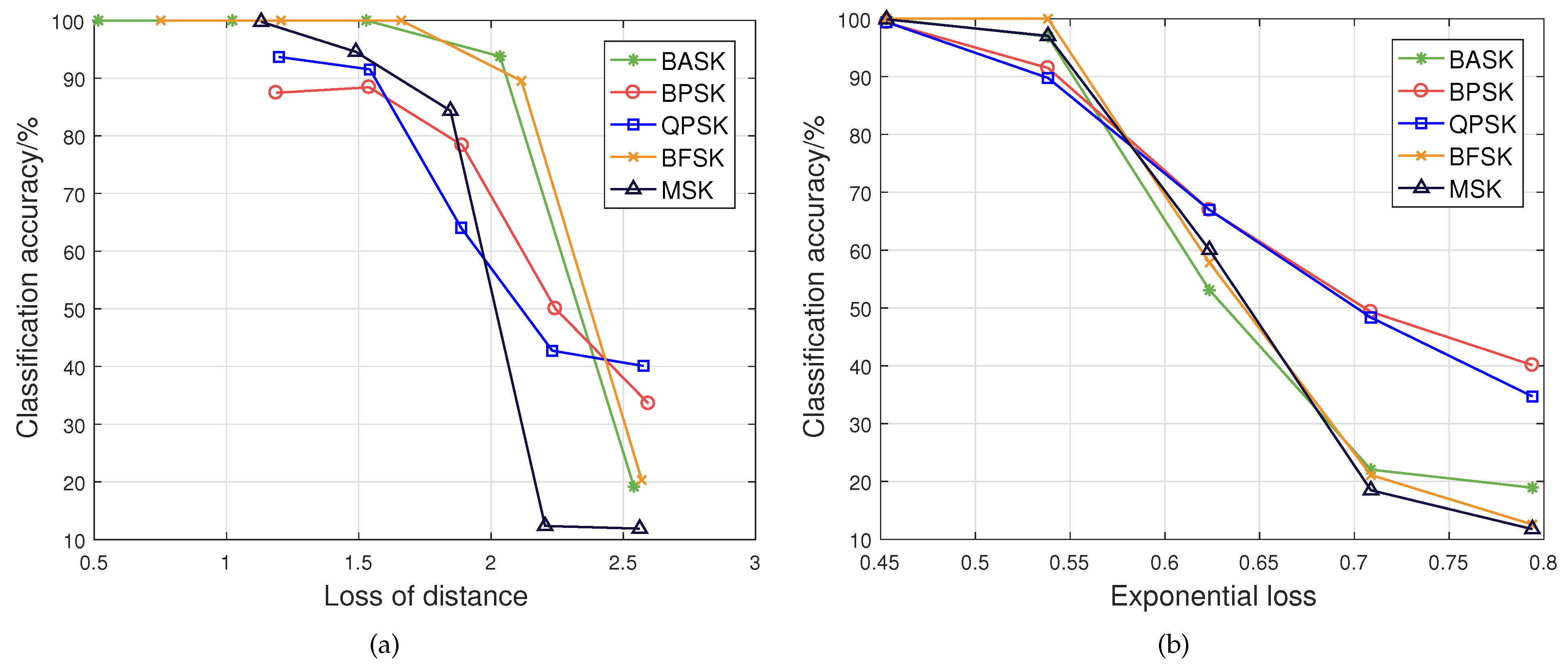
The values of the two loss functions under various modulation schemes and SNRs are shown in Figure 4. It is obvious that both the loss of distance and exponential loss decrease with the increase in the SNR of the received signal. This is because the signal features of the received signal are not significantly affected by noise under low SNR. In addition, it is observed that both the loss of distance and exponential loss of BASK and BFSK modulation schemes are smaller than those of other modulation schemes under the same SNR of the received signal. Since the unique signal features can be obtained at both spectral and cyclic frequencies under BASK and BFSK modulation schemes, the BASK and BFSK modulation schemes have less value of loss function and are easier to be classified than the other modulation schemes, as analyzed in Section 3.3. Then, the classification accuracies under different values of loss function are shown in Figure 5. It is obvious that the classification accuracy declines with the increase in the loss of distance or exponential loss under each modulation scheme. In particular, the classification accuracy decreases sharply when the loss of distance is greater than a certain threshold, which indicates that the signal feature cannot be distinguished accurately when the received signal is too weak.

In the proposed distributed Co-AMC network, the SNR of the received signal at each node is different and varies with time due to the geographical distribution of nodes and the impact of multipath fading channels. The classification performance of the whole network will be affected if the local decision is fused, which is obtained from the node with too low SNR of the current received signal. Thus, the reliability of the local decision is designed as the weighted value when that is fused according to the two loss functions. We set a threshold for loss of distance and exponential loss, respectively. When the values of loss functions are lower than their threshold, the current local decision is considered reliable, i.e., the weighted value is one, Otherwise, the weighted value is zero. Thus, we have

$$w_i=\left\{\begin{array}{c}1,l_{dist}\le {\epsilon }_{dist},l_{exp}\le {\epsilon }_{exp},\hfill \\ 0,\mathrm{otherwise},\hfill \end{array}\right.$$

(26)

where $w_i,\forall i\in \mathcal{V}$ represents the reliability of the i-th node, ${\epsilon }_{dist}$ and ${\epsilon }_{exp}$ represent the threshold of the loss of distance and the exponential loss, respectively. Finally, ${\left\{\left(Y_i,w_i\right)\right\}}_{i=1}^I$ are the local decision and its corresponding reliability obtained by each node, which are iteratively exchanged for decision fusion in the proposed network.

3.6. Decision Fusion Module

In this section, we introduce the decision fusion module based on the designed DWA-ADMM algorithm. In Section 3.4 and Section 3.5, the local decision and the reliability of each node which can be transmitted to other connected nodes with communication links in the proposed network have been obtained through the KNN-based classifier. In order to compute the unified global classification result, the local decisions are weighted and averaged according to their reliabilities through their iterative exchange among connected nodes in the designed decision fusion module based on ADMM.

Considering problem (4) mentioned in Section 2, the core idea of the ADMM algorithm is the augmented Lagrange method (ALM) of the original dual algorithm [36]. In addition, in order to accelerate the convergence speed of the algorithm, the penalty function is applied. The augmented Lagrange function of problem (4) is

$$\begin{array}{cc}\hfill L_{\rho }\left(\left\{x_i\right\},\left\{z_{ij}\right\},\left\{u_{ij}\right\},\left\{v_{ij}\right\}\right)& =\sum _i^I{f}_i\left(x_i\right)+\sum _{i=1}^I\sum _{j\in {\mathcal{N}}_i}\left[u_{ij}^T\left(x_i-z_{ij}\right)+v_{ij}^T\left(x_j-z_{ij}\right)\right]\hfill \\ \hfill & +\frac{\rho }{2}\sum _{i=1}^I\sum _{j\in {\mathcal{N}}_i}\left[{∥x_i-z_{ij}∥}_2^2+{∥x_j-z_{ij}∥}_2^2\right],\hfill \end{array}$$

(27)

where $u_{ij}$ and $v_{ij}$ are Lagrange dual variables corresponding to the two constraints $x_i=z_{ij}$ and $x_j=z_{ij}$, respectively, $\rho$ is the penalty parameter and the last term is the $l_2$-norm of the two constraints which is used to promote robustness. The ADMM algorithm is solved iteratively by updating the variable $\left\{x_i\right\}$, $\left\{z_{ij}\right\}$, $\left\{u_{ij}\right\}$ and $\left\{v_{ij}\right\}$ according to the following rule [36]:

$$\begin{array}{cc}\hfill x_i^{\left(t+1\right)}& =\arg \underset{x_i}{\min }\left[f_i\left(x_i\right)+\sum _{j\in {\mathcal{N}}_i}\left(u_{ij}^{\left(t\right)T}{x}_i+v_{ij}^{\left(t\right)T}{x}_j\right)\right.\hfill \\ \hfill & \left.+\frac{\rho }{2}\sum _{j\in {\mathcal{N}}_i}\left({∥x_i-z_{ij}^{\left(t\right)}∥}_2^2+{∥x_j-z_{ij}^{\left(t\right)}∥}_2^2\right)\right],\forall i\in \mathcal{V},\hfill \end{array}$$

(28)

$$\begin{array}{cc}\hfill z_{ij}^{\left(t+1\right)}& =\arg \underset{z_{ij}}{\min }\left[u_{ij}^{\left(t\right)T}\left(x_i^{\left(t+1\right)}-z_{ij}\right)\right.+v_{ij}^{\left(t\right)T}\left(x_j^{\left(t+1\right)}-z_{ij}\right)\hfill \\ \hfill & \left.+\frac{\rho }{2}\left({∥x_i^{\left(t+1\right)}-z_{ij}∥}_2^2+{∥x_j^{\left(t+1\right)}-z_{ij}∥}_2^2\right)\right],\forall i\in \mathcal{V},\forall j\in {\mathcal{N}}_i,\hfill \end{array}$$

(29)

$$u_{ij}^{\left(t+1\right)}=u_{ij}^{\left(t\right)}+\rho \left[x_i^{\left(t+1\right)}-z_{ij}^{\left(t+1\right)}\right],$$

(30)

$$v_{ij}^{\left(t+1\right)}=v_{ij}^{\left(t\right)}+\rho \left[x_j^{\left(t+1\right)}-z_{ij}^{\left(t+1\right)}\right].$$

(31)

At the t-th iteration and for $\forall i\in \mathcal{V},\forall j\in {\mathcal{N}}_i$, each variable is updated alternately by fixing other variables. In order to simplify the above update rule, it is worth noting that (29) is a quadratic unconstrained equation about $z_{ij}$, whose closed solution is

$$z_{ij}^{\left(t+1\right)}=\frac{1}{2}\left(x_i^{\left(t+1\right)}+x_j^{\left(t+1\right)}\right)+\frac{1}{2\rho }\left(u_{ij}^{\left(t\right)}+v_{ij}^{\left(t\right)}\right).$$

(32)

By substituting (32) into (30) and (31), and setting $u_{ij}^{\left(0\right)}=v_{ij}^{\left(0\right)}=0$, (30) and (31) can be simplified as

$$u_{ij}^{\left(t+1\right)}=u_{ij}^{\left(t\right)}+\frac{\rho }{2}\left[x_i^{\left(t+1\right)}-x_j^{\left(t+1\right)}\right],$$

(33)

$$v_{ij}^{\left(t+1\right)}=v_{ij}^{\left(t\right)}+\frac{\rho }{2}\left[x_j^{\left(t+1\right)}-x_i^{\left(t+1\right)}\right].$$

(34)

Meanwhile, it is obvious that $u_{ij}^{\left(t\right)}=-v_{ij}^{\left(t\right)}$ and $u_{ij}^{\left(t\right)}=v_{ji}^{\left(t\right)}$ at any iteration. Thus, (32) can be further simplified as

$$z_{ij}^{\left(t\right)}=\frac{1}{2}\left(x_i^{\left(t\right)}+x_j^{\left(t\right)}\right).$$

(35)

At the t-th iteration and for $\forall i\in \mathcal{V},\forall j\in {\mathcal{N}}_i$, by substituting (35) into (28) and defining $p_i^{\left(t\right)}\stackrel{\Delta }{=}\sum _{j\in {\mathcal{N}}_i}\left(u_{ij}^{\left(t\right)}+v_{ij}^{\left(t\right)}\right)$ as the Lagrange multiplier with the initial condition $p_i^{\left(0\right)}=0$, the update rule of the ADMM can be simplified as

$$\begin{array}{cc}\hfill x_i^{\left(t+1\right)}& =\arg \underset{x_i}{\min }\left[f_i\left(x_i\right)+p_i^{\left(t\right)T}{x}_i\right.\left.+\rho \sum _{j\in {\mathcal{N}}_i}\left({∥x_i-\frac{1}{2}\left(x_i^{\left(t\right)}+x_j^{\left(t\right)}\right)∥}_2^2\right)\right],\hfill \end{array}$$

(36)

$$p_i^{\left(t+1\right)}=p_i^{\left(t\right)}+\rho \sum _{j\in {\mathcal{N}}_i}\left(x_i^{\left(t+1\right)}-x_j^{\left(t+1\right)}\right),\forall i\in \mathcal{V}.$$

(37)

In the above algorithm, each node stores the variable $x_i$ and the corresponding Lagrange multiplier $p_i$. In each iteration, the i-th node receives the estimated variable $x_j^{\left(t\right)},j\in {\mathcal{N}}_i$ from the connected nodes and optimizes the local objective function $f_i\left(x_i\right)$. Then the i-th node shares the updated estimated variables with the connected nodes for the next iteration. In this paper, the local objective function can be expressed as

$$f_i\left(x_i\right)=\sum _{m=1}^M{∥w_i^T{x}_{im}-y_{im}∥}_2^2,\forall i\in \mathcal{V},$$

(38)

where $x_i\in \left\{x_{i1},x_{i2},\dots ,x_{iM}\right\}$ is the estimated variable, $y_{im},m=1,2,\dots ,M$ is the local decision obtained by the classifier in the i-th node, and $w_i$ is the corresponding reliability. Therefore, problem (4) can be specifically expressed as

$$\begin{array}{c}\underset{\left\{x_i\right\}}{\min }{\displaystyle \sum _{i=1}^I}{\displaystyle \sum _{m=1}^M}{∥w_i{x}_{im}-y_{im}∥}_2^2,\hfill \\ s.t.x_{im}=z_{ij},x_{jm}=z_{ij},\forall i,\forall j\in {\mathcal{N}}_i.\hfill \end{array}$$

(39)

The global optimization objective of (39) is to compute the weighted average of local decisions obtained by all nodes in the network according to their reliabilities. By substituting (39) into (36) and (37), the update rule of the DWA-ADMM can be expressed as

$$x_{im}^{\left(t+1\right)}=\left(y_{im}{w}_i-\frac{p_{im}^{\left(t\right)}}{2}+\frac{\rho }{2}\left|{\mathcal{N}}_i\right|+\frac{\rho }{2}\sum _{\forall j\in {\mathcal{N}}_i}{x}_{jm}^{\left(t\right)}\right)/\phantom{\left(y_{im}{w}_i-\frac{p_{im}^{\left(t\right)}}{2}+\frac{\rho }{2}\left|{\mathcal{N}}_i\right|+\frac{\rho }{2}\sum _{\forall j\in {\mathcal{N}}_i}{x}_{jm}^{\left(t\right)}\right)\left(w_i^2+\rho \left|{\mathcal{N}}_i\right|\right)}\left(w_i^2+\rho \left|{\mathcal{N}}_i\right|\right),$$

(40)

$$\begin{array}{cc}\hfill p_{im}^{\left(t+1\right)}& =p_{im}^{\left(t\right)}+\rho \left(\left|{\mathcal{N}}_i\right|x_i^{\left(t+1\right)}-\sum _{j\in {\mathcal{N}}_i}{x}_j^{\left(t+1\right)}\right),\forall i\in \mathcal{V},i=1,2,\dots ,M.\hfill \end{array}$$

(41)

Meanwhile, we use the primal residuals $r_{im},\forall i\in \mathcal{V},m=1,2,\dots ,M$ and dual residuals $s_{im},\forall i\in \mathcal{V},m=1,2,\dots ,M$ as the variables to decide when the iteration stops, which can be expressed as

$$r_{im}^{\left(t+1\right)}=\left|{\mathcal{N}}_i\right|x_{im}^{\left(t+1\right)}-\sum _{j\in {\mathcal{N}}_i}{x}_j^{\left(t+1\right)},$$

(42)

$$s_{im}^{\left(t+1\right)}=\rho y_{im}{w}_i\left(\sum _{j\in {\mathcal{N}}_i}{x}_j^{\left(t+1\right)}-\sum _{j\in {\mathcal{N}}_i}{x}_j^{\left(t\right)}\right).$$

(43)

Note that the iteration of the proposed DWA-ADMM algorithm will stop when the $l_2$-norm of primal residuals and dual residuals are lower than the predetermined thresholds in all nodes, which can be expressed as

$$\sum _{m=1}^M{∥r_{im}^{\left(t\right)}∥}_2^2\le {\epsilon }^{\mathrm{pri}},$$

(44)

$$\sum _{m=1}^M{∥s_{im}^{\left(t\right)}∥}_2^2\le {\epsilon }^{dual},$$

(45)

where ${\epsilon }^{\mathrm{pri}}$ and ${\epsilon }^{dual}$ represent the predetermined thresholds of the primal residual and dual residual, respectively. Finally, after the iteration, the estimated variables $x_{1m}=x_{im}=x_{Im}$ represent the possibility that the modulation scheme of the received signal belongs to class ${\omega }_m$. In the proposed distributed Co-AMC network, the unified classification result of the received signal is the class corresponding to the maximum value in $x_i\in \left\{x_{i1},x_{i2},\dots ,x_{iM}\right\}$, which can be expressed as

$${\omega }_r=\arg \underset{x_{im}}{\max }\left\{x_{im},{\omega }_m\right\},m=1,2,\dots ,M,$$

(46)

The proposed DWA-ADMM procedure can be summarized in Algorithm 2.

Algorithm 2: The Proposed DWA-ADMM

Input:    (1) The local decision $Y_i\in \left\{y_{i1},y_{i2},\dots ,y_{iM}\right\},\forall i\in \mathcal{V}$;    (2) The reliability of the local decision $w_i,\forall i\in \mathcal{V}$;    (3) The penalty parameter $\rho$.    Output:    The classification result ${\omega }_r$.

In addition, we can also impose the following standard propositions on the optimization problem in (38).

Proposition 1.

(Convexity): Each of the objective functions $f_i\left(x_i\right)$ is closed, proper and strictly convex.

Proposition 2.

(Existence of a Saddle Point): The unaugmented Lagrange function of problem (38), $L\left(x_i,z_{ij},p_i\right)$, has a saddle point, i.e., there exists a solution $\left(x_i^{*},z_{{}_{ij}}^{*},p_i\right)$, not necessarily unique, for which $L\left(x_i^{*},z_{{}_{ij}}^{*},p_i\right)\le L\left(x_i^{*},z_{{}_{ij}}^{*},p_i^{*}\right)\le L\left(x_i,z_{ij},p_i^{*}\right),\forall i\in \mathcal{V}$.

The proof of the convexity is well known and can be found in [37] and the proof of the existence of the saddle point can be found in [38]. Since the objective function of (38) is affine, i.e., satisfying all those conditions, the algorithm is guaranteed to converge. Hence, this convergence property is independent of the network topology, and, in essence, it highlights the application of the proposed algorithm to the arbitrarily connected networks.

4. Experimental Results

In this section, we conduct experiments to verify the effectiveness of the key components in the proposed distributed Co-AMC network. Specifically, in Section 4.1, we focus on analyzing the complexity and convergence of the designed algorithm. In Section 4.2 and Section 4.3, the accuracy of the proposed network for modulation classification is evaluated by comparing with AMC of a single node and other existing methods. Furthermore, in Section 4.4, we analyze the impact of the number of nodes and the connectivity of the communication network on the performance of the proposed distributed Co-AMC network. For a fair comparison, all the algorithms are implemented using a Matlab 2019b/Windows 10 environment on a computer with a 2.10 GHz AMD-Ryzen-3500U.

4.1. Computational Complexity and Convergence Property of the Distributed Co-AMC Network

The overall computational complexity of each node in the proposed network consists of three parts. Firstly, the cyclic spectrum is calculated from the received signal with $N_r$ samples according to the FAM method. Then, the local decision and its reliability are obtained by computing and searching K-nearest neighbors in the training dataset, in which there are $L_{Tr}$ training samples with length $N_{Tr}$. Thirdly, the classification result is obtained through $T_i$-times iterative computation from the M-dimension local decision in the proposed network with I nodes. The complexity of the three steps can be expressed as $\mathcal{O}\left(N_r^2+N_r{\log }_2\left(N_r\right)\right)$, $\mathcal{O}\left(L_{Tr}{N}_{Tr}+K{N}_{Tr}\right)$ and $\mathcal{O}\left(T_i\left(M^2+MI\right)\right)$, respectively.

Compared with the other two steps, the second step has the highest computational complexity, which mainly depends on the sizes of the training dataset and training sample. However, benefiting from the resampling and quantization in the feature extraction module, the size of the training sample is much less than the received signal, i.e., $N_{Tr}\ll N_r$, and the training sample contains the values of zero, which significantly reduce the computational complexity in the second step. In addition, in the third step, the designed algorithm for decision fusion further reduces the computational complexity by reducing the amount of complex multiplication in each iteration.

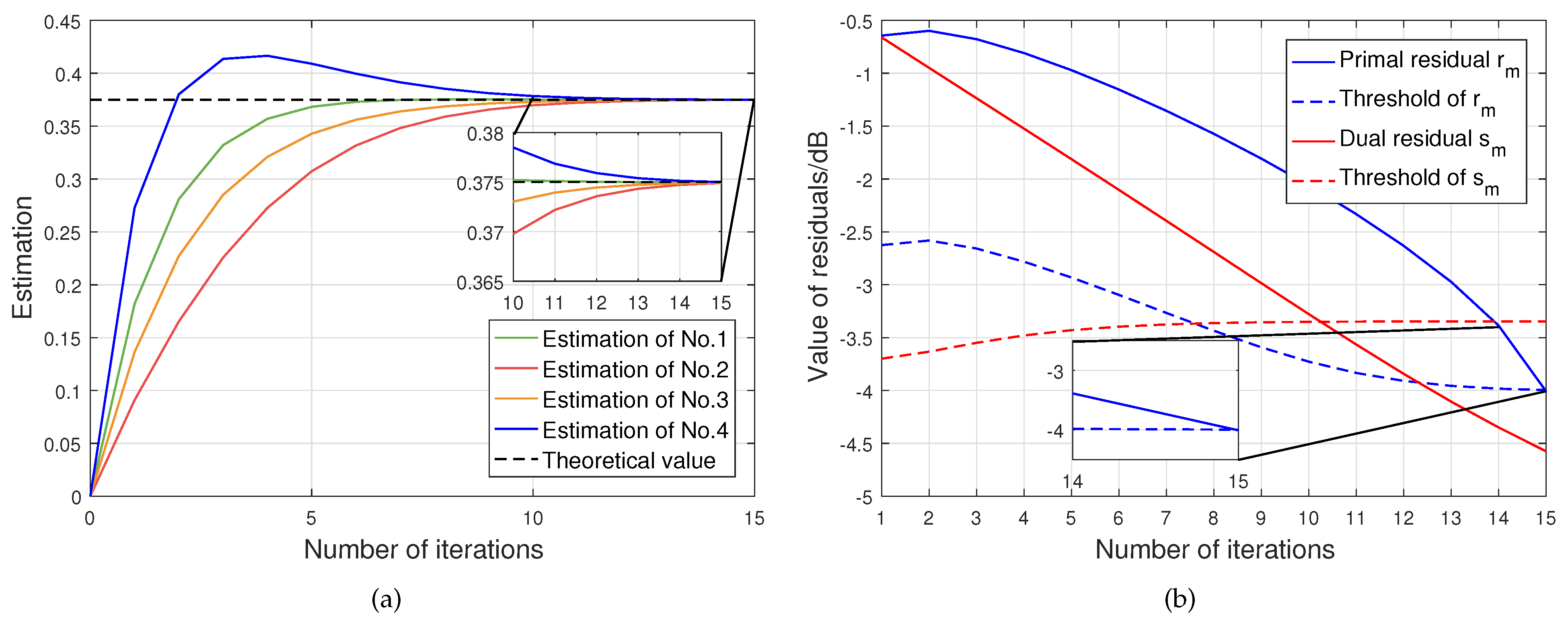
In addition, in order to evaluate the convergence property of the designed DWA-ADMM algorithm, we carry out a simulation experiment for the decision fusion module. We randomly generate the local decisions and their corresponding reliability for each node in the network, and fuse them by iterative computation according to the algorithm introduced in Section 3.6. In this experiment, we assume that the number of nodes $I=4$ and the network is fully connected, which means that each node can connect with all other nodes. According to (39), the theoretical value of the fused decision for the class is the weighted average of local decisions for each node, i.e., ${\overline{y}}_m={\sum }_{i=1}^I{w}_i{y}_{im}/\phantom{{\sum }_{i=1}^I{w}_i{y}_{im}{\sum }_{i=1}^I{w}_i}{\sum }_{i=1}^I{w}_i$. The objective of each node is to make the estimation close to the theoretical value by iteration.

The convergence results of each node are presented in Figure 6. It can be observed that the estimations of all nodes in the network, whose initial values are zero, are almost equal to the theoretical value after fifteen iterations, as shown in Figure 6a. Furthermore, in Figure 6b, it can be observed that the iteration stops when the primal residual and dual residual of the estimation are both less than their respective thresholds according to (44) and (45).

4.2. Classification Effectiveness of the Distributed Co-AMC Network

To assess the effectiveness of the proposed distributed Co-AMC network, the following metrics are considered: accuracy, precision, and recall, as defined in Equations (47)–(49), respectively. These metrics are derived from the confusion matrix, which includes true positive (TP), false positive (FP), false negative (FN), and true negative (TN) indices. TP and TN represent the number of positive and negative samples correctly classified, while FP and FN represent the number of positive and negative samples incorrectly classified. In addition, we randomly generate 1000 sets of testing samples for each class under various SNRs to verify the performance of the proposed distributed Co-AMC network according to the dataset parameters in Section 3.2.

$$Accuracy=\frac{TP+TN}{TP+FP+TN+FN},$$

(47)

$$Precision=\frac{TP}{TP+FP},$$

(48)

$$Recall=\frac{TP}{TP+FN}.$$

(49)

To measure the accuracy of the proposed distributed Co-AMC network, we employ the confusion matrix. The obtained confusion matrix is presented in Figure 7. In this figure, the first five diagonal cells show the number and percentage of correct classifications by the proposed network. For example, 1000 testing samples are correctly classified as a BASK modulation scheme, which corresponds to 20.0% of all 5000 testing samples. The observation reveals that the predicted and actual classes tend to cluster along the diagonal axes, indicating a high classification accuracy achieved by the proposed network. Meanwhile, the blue cells (except the diagonals) show the number and percentage of incorrect classifications. For example, 66 testing samples of the BPSK modulation scheme are incorrectly classified as the QPSK modulation scheme, which corresponds to 1.3% of all testing samples. In addition, the green cells on the right and bottom display the precision and recall metrics for each classification. Specifically, out of 1004 predictions of the BASK modulation scheme, 99.6% are correct and 0.4% are wrong, according to (48). Similarly, out of 1000 testing samples of the BPSK modulation scheme, 89.8% are correctly classified as the BPSK modulation scheme and 10.2% are classified as other modulation schemes, according to (49).

Overall, 92.7% of the predictions are classified correctly and 7.3% are wrong classifications, as shown in the green cell at the bottom right. The best-classified modulation schemes are BASK and BFSK with a recall of 100%, while the class classification error of the proposed network mainly occurs for the BPSK, QPSK, and MSK modulation schemes. This is because the extracted signal features of BASK and BFSK can be distinguished in both spectral frequency and cyclic frequency, while the extracted features of other classifications only have significant differences in cyclic frequency, especially under low SNRs.

4.3. Classification Accuracy of the Distributed Co-AMC Compared to the Single-Node AMC and Existing AMC Methods

To assess the classification accuracy of the proposed distributed Co-AMC network in comparison to the single-node AMC, an ablation study is conducted. In the single-node AMC, the local decision of a single node is considered to be the classification result. The accuracies of the Co-AMC and single-node AMC are compared and depicted in Figure 8. The results demonstrate that the proposed distributed Co-AMC network significantly outperforms the single-node AMC across various modulation schemes and SNRs. Notably, with the distributed Co-AMC network, the classification accuracy not only increases with the increase in SNR but also achieves near 100% when the SNR is as low as 0 dB for specific modulation schemes. Due to the geographical distribution of nodes and the impact of multipath fading channels in the Co-AMC network with multiple nodes, the SNR of the received signal at each node is different and varies with time, which will affect the classification accuracy if only the local decision from one node is used as the classification result of the whole network. Benefiting from the designed decision fusion module based on DWA-ADMM, the local decisions from all nodes are weighted and averaged based on their reliabilities, which filters those from the nodes with low SNR and improves the classification accuracy.

Furthermore, the classification accuracies of the proposed distributed Co-AMC network, as compared to other methods, are presented in Figure 9. The existing AMC method introduced in [39] is used as a baseline for comparison. The results demonstrate that the proposed distributed Co-AMC network outperforms existing methods significantly across various modulation schemes and SNRs. Remarkably, the proposed distributed Co-AMC network demonstrates a significant improvement in classification accuracy with increasing SNR. Particularly, under BFSK modulation schemes, the accuracy reaches nearly 100% even at an extremely low SNR of −15 dB. Similarly, under BPSK, QPSK, and MSK modulation schemes, the accuracy achieves 90% at a challenging SNR as low as −10 dB, which cannot be achieved by the existing method under such a low SNR. Thus, our proposed network is more suitable for AMC under the condition of low SNR.

4.4. Classification Effectiveness of the Distributed Co-AMC Network with Different Numbers of Nodes and Connectivity

To verify the robustness of our proposed network under different network scales and topologies, we apply the designed DWA-ADMM algorithm to the architecture with different numbers of nodes and connectivities, where the number of nodes and its connectivity correspond to the network scale and topology, respectively, as mentioned in Section 2.

The classification accuracy and the number of iterations of our proposed network with different numbers of nodes under various SNRs are shown in Figure 10. It can be observed that the classification accuracy of the network with a different number of nodes rises with the increase in SNR and reaches almost 100% when the SNR is as low as −5 dB∼0 dB. Noticeably, the classification accuracy of the network with a larger number of nodes is higher than those with fewer nodes when the SNR is lower than 0dB. In contrast, the number of iterations first decreases and then remains stable with the increase in SNR. Meanwhile, the number of iterations with a larger number of nodes is higher than those with fewer nodes when the SNR is small, which means that the expansion of the network scale increases the number of iterations while improving the classification performance, especially under low SNR. This is because the reliabilities of local decisions become one with the increase in the average SNR of all nodes in the network. The theoretical value of the fused decision degenerates from the weighted average to the arithmetic average, i.e., ${\overline{y}}_m={\sum }_{i=1}^I{y}_{im}/\phantom{{\sum }_{i=1}^I{y}_{im}I}I$, which reduces the computational complexity of the optimization objective function and thus reduces the number of iterations.

In addition, the number of iterations of the network with a different number of nodes and its connectivity are shown in Figure 11. It is observed that the number of iterations gradually decreases and stabilizes with the increase in connectivity. This indicates that our proposed distributed Co-AMC network can achieve a reliable classification result with a few iterations without establishing too many communication connections among nodes. Therefore, the proposed distributed Co-AMC is adaptive to wireless networks with various scales and topologies.

5. Conclusions

In this paper, we have proposed a novel distributed Co-AMC network based on ML for wireless communication networks. The proposed network architecture consists of four essential modules: the feature extraction module, classifier module, reliability estimation module, and decision fusion module. Specifically, the feature vectors with resampling and quantization were calculated by applying the cyclic spectrum to the feature extraction module. The classifier module based on the KNN was designed to obtain the local decision according to the feature vectors at each distributed node. Then, the reliability of the local decision was estimated by applying two loss functions in the reliability estimation module. Finally, the classification result of the modulation scheme was obtained by applying the designed DWA-ADMM algorithm through iterative calculation among distributed nodes. Simulation results demonstrated that the proposed distributed Co-AMC network outperformed the existing AMC methods under various modulation schemes, especially when the SNR was low. In addition, our proposed Co-AMC is adaptive to the variations in the number of nodes and topologies of wireless networks, thereby possessing higher flexibility and practicability.

References

- Qi, P.; Zhou, X.; Zheng, S.; Li, Z. Automatic modulation classification based on deep residual networks with multimodal information. IEEE Trans. Cogn. Commun. Netw. 2020, 7, 21–33. [Google Scholar] [CrossRef]
- Jafar, N.; Paeiz, A.; Farzaneh, A. Automatic modulation classification using modulation fingerprint extraction. J. Syst. Eng. Electron. 2021, 32, 799–810. [Google Scholar] [CrossRef]
- Kojima, S.; Maruta, K.; Feng, Y.; Ahn, C.J.; Tarokh, V. CNN-based joint SNR and Doppler shift classification using spectrogram images for adaptive modulation and coding. IEEE Trans. Commun. 2021, 69, 5152–5167. [Google Scholar] [CrossRef]
- Peng, S.; Sun, S.; Yao, Y.D. A survey of modulation classification using deep learning: Signal representation and data preprocessing. IEEE Trans. Neural Netw. Learn. Syst. 2021, 33, 7020–7038. [Google Scholar] [CrossRef] [PubMed]
- Dobre, O.A.; Abdi, A.; Bar-Ness, Y.; Su, W. Survey of automatic modulation classification techniques: Classical approaches and new trends. IET Commun. 2007, 1, 137–156. [Google Scholar] [CrossRef] [Green Version]
- Ozdemir, O.; Wimalajeewa, T.; Dulek, B.; Varshney, P.K.; Su, W. Asynchronous linear modulation classification with multiple sensors via generalized EM algorithm. IEEE Trans. Wirel. Commun. 2015, 14, 6389–6400. [Google Scholar] [CrossRef] [Green Version]
- Yan, X.; Feng, G.; Wu, H.C.; Xiang, W.; Wang, Q. Innovative robust modulation classification using graph-based cyclic-spectrum analysis. IEEE Commun. Lett. 2016, 21, 16–19. [Google Scholar] [CrossRef]
- Zhang, Q.; Guan, Y.; Li, H.; Xiong, K.; Song, Z. Distributed deep learning-based signal classification for time–frequency synchronization in wireless networks. Comput. Commun. 2023, 201, 37–47. [Google Scholar] [CrossRef]
- Wang, F.; Huang, S.; Wang, H.; Yang, C. Automatic modulation classification exploiting hybrid machine learning network. Math. Probl. Eng. 2018, 2018, 1–14. [Google Scholar] [CrossRef]
- Kumar, Y.; Sheoran, M.; Jajoo, G.; Yadav, S.K. Automatic modulation classification based on constellation density using deep learning. IEEE Commun. Lett. 2020, 24, 1275–1278. [Google Scholar] [CrossRef]
- Abdelbar, M.; Tranter, W.H.; Bose, T. Cooperative cumulants-based modulation classification in distributed networks. IEEE Trans. Cogn. Commun. Netw. 2018, 4, 446–461. [Google Scholar] [CrossRef]
- Abdelgawad, A.; Bayoumi, M. Resource-Aware Data Fusion Algorithms for Wireless Sensor Networks; Springer Science & Business Media: Berlin/Heidelberg, Germany, 2012; Volume 118. [Google Scholar]
- Hakimi, S.; Hodtani, G.A. Optimized distributed automatic modulation classification in wireless sensor networks using information theoretic measures. IEEE Sens. J. 2017, 17, 3079–3091. [Google Scholar] [CrossRef]
- Wang, Y.; Wang, J.; Zhang, W.; Yang, J.; Gui, G. Deep learning-based cooperative automatic modulation classification method for MIMO systems. IEEE Trans. Veh. Technol. 2020, 69, 4575–4579. [Google Scholar] [CrossRef]
- Ozdemir, O.; Li, R.; Varshney, P.K. Hybrid maximum likelihood modulation classification using multiple radios. IEEE Commun. Lett. 2013, 17, 1889–1892. [Google Scholar] [CrossRef] [Green Version]
- Dulek, B.; Ozdemir, O.; Varshney, P.K.; Su, W. Distributed maximum likelihood classification of linear modulations over nonidentical flat block-fading Gaussian channels. IEEE Trans. Wirel. Commun. 2014, 14, 724–737. [Google Scholar] [CrossRef]
- Dulek, B. An online and distributed approach for modulation classification using wireless sensor networks. IEEE Sens. J. 2017, 17, 1781–1787. [Google Scholar] [CrossRef]
- Headley, W.C.; Reed, J.D.; da Silva, C.R.C.M. Distributed Cyclic Spectrum Feature-Based Modulation Classification. In Proceedings of the 2008 IEEE Wireless Communications and Networking Conference, Las Vegas, NV, USA, 31 March–3 April 2008; pp. 1200–1204. [Google Scholar] [CrossRef]
- Fu, X.; Gui, G.; Wang, Y.; Gacanin, H.; Adachi, F. Automatic modulation classification based on decentralized learning and ensemble learning. IEEE Trans. Veh. Technol. 2022, 71, 7942–7946. [Google Scholar] [CrossRef]
- Yan, X.; Rao, X.; Wang, Q.; Wu, H.C.; Zhang, Y.; Wu, Y. Novel Cooperative Automatic Modulation Classification Using Unmanned Aerial Vehicles. IEEE Sens. J. 2021, 21, 28107–28117. [Google Scholar] [CrossRef]
- Wang, Y.; Guo, L.; Zhao, Y.; Yang, J.; Adebisi, B.; Gacanin, H.; Gui, G. Distributed learning for automatic modulation classification in edge devices. IEEE Wirel. Commun. Lett. 2020, 9, 2177–2181. [Google Scholar] [CrossRef]
- Tian, Z.; Zhang, Z.; Wang, J.; Chen, X.; Wang, W.; Dai, H. Distributed ADMM with synergetic communication and computation. IEEE Trans. Commun. 2020, 69, 501–517. [Google Scholar] [CrossRef]
- Zhang, Q.; Wang, J.; Wang, Y. Efficient QAM signal detector for massive MIMO systems via PS/DPS-ADMM approaches. IEEE Trans. Wirel. Commun. 2022, 21, 8859–8871. [Google Scholar] [CrossRef]
- Manosha, K.S.; Joshi, S.K.; Codreanu, M.; Rajatheva, N.; Latva-aho, M. Admission control algorithms for QoS-constrained multicell MISO downlink systems. IEEE Trans. Wirel. Commun. 2017, 17, 1982–1999. [Google Scholar] [CrossRef] [Green Version]
- Leinonen, M.; Codreanu, M.; Juntti, M. Distributed joint resource and routing optimization in wireless sensor networks via alternating direction method of multipliers. IEEE Trans. Wirel. Commun. 2013, 12, 5454–5467. [Google Scholar] [CrossRef]
- Strom, E.G.; Malmsten, F. A maximum likelihood approach for estimating DS-CDMA multipath fading channels. IEEE J. Sel. Areas Commun. 2000, 18, 132–140. [Google Scholar] [CrossRef]
- Yi, Z.; Jiao, Y.; Dai, W.; Li, G.; Wang, H.; Xu, Y. A Stackelberg Incentive Mechanism for Wireless Federated Learning With Differential Privacy. IEEE Wirel. Commun. Lett. 2022, 11, 1805–1809. [Google Scholar] [CrossRef]
- Li, T.; Fu, M.; Xie, L.; Zhang, J.F. Distributed consensus with limited communication data rate. IEEE Trans. Autom. Control 2010, 56, 279–292. [Google Scholar] [CrossRef] [Green Version]
- Fiedler, M. Algebraic connectivity of graphs. Czechoslov. Math. J. 1973, 23, 298–305. [Google Scholar] [CrossRef]
- Gardner, W. Spectral correlation of modulated signals: Part I-analog modulation. IEEE Trans. Commun. 1987, 35, 584–594. [Google Scholar] [CrossRef]
- Gardner, W.; Brown, W.; Chen, C.K. Spectral correlation of modulated signals: Part II-digital modulation. IEEE Trans. Commun. 1987, 35, 595–601. [Google Scholar] [CrossRef]
- Gardner, W. Measurement of spectral correlation. IEEE Trans. Acoust. Speech Signal Process. 1986, 34, 1111–1123. [Google Scholar] [CrossRef]
- Tom, C. Cyclostionary Spectral Analysis of Typical Satcom Signals Using the fft Accumulation Method; Technical Report; Defence Research Establishment Ottawa (Ontario): Ottawa, ON, Canada, 1995. [Google Scholar]
- Zhang, S.; Li, X.; Zong, M.; Zhu, X.; Cheng, D. Learning k for knn classification. ACM Trans. Intell. Syst. Technol. (TIST) 2017, 8, 1–19. [Google Scholar] [CrossRef] [Green Version]
- Zhang, S. Challenges in KNN Classification. IEEE Trans. Knowl. Data Eng. 2022, 34, 4663–4675. [Google Scholar] [CrossRef]
- Boyd, S.; Parikh, N.; Chu, E.; Peleato, B.; Eckstein, J. Distributed optimization and statistical learning via the alternating direction method of multipliers. Found. Trends® Mach. Learn. 2011, 3, 1–122. [Google Scholar]
- Goldsmith, A. Wireless Communications; Cambridge University Press: Cambridge, UK, 2005. [Google Scholar]
- Foukalas, F.; Shakeri, R.; Khattab, T. Distributed power allocation for multi-flow carrier aggregation in heterogeneous cognitive cellular networks. IEEE Trans. Wirel. Commun. 2018, 17, 2486–2498. [Google Scholar] [CrossRef]
- Ma, J.; Qiu, T. Automatic modulation classification using cyclic correntropy spectrum in impulsive noise. IEEE Wirel. Commun. Lett. 2018, 8, 440–443. [Google Scholar] [CrossRef]
Figure 1.
Architecture of the distributed wireless transceiver platform.
Figure 2.
Architecture of the proposed distributed Co-AMC network.
Figure 3.
Architecture of the feature extraction module.
Figure 4.
Two loss functions under various modulation schemes and SNRs. (a) Loss of distance. (b) Exponential loss.
Figure 5.
Classification accuracy under two loss functions. (a) Classification accuracy under different loss of distance. (b) Classification accuracy under different exponential loss.
Figure 6.
Convergence results of the designed DWA-ADMM algorithm. (a) Estimated result of the local decision in each node. (b) Residuals of estimation in each node.
Figure 7.
Confusion matrix of the classification result.
Figure 8.
Classification accuracy of Co-AMC compared with the single-node AMC.
Figure 9.
Classification accuracy of Co-AMC compared with the existing AMC methods.
Figure 10.
Classification accuracy and number of iterations for the network with different numbers of nodes.
Figure 11.
Number of iterations for the network with different numbers of nodes and connectivities.