Support Vector Regression Model for Determining Optimal Parameters of HfAlO-Based Charge Trapping Memory Devices

Abstract

The production and optimization of HfAlO-based charge trapping memory devices is central to our research. Current optimization methods, based largely on experimental experience, are tedious and time-consuming. We examine various fabrication parameters and use the resulting memory window data to train machine learning algorithms. An optimized Support Vector Regression model, processed using the Swarm algorithm, is applied for data prediction and process optimization. Our model achieves a MSE of 0.47, an R² of 0.98856, and a recognition accuracy of 90.3% under cross-validation. The findings underscore the effectiveness of machine learning algorithms in non-volatile memory fabrication process optimization, enabling efficient parameter selection or outcome prediction.

1. Introduction

Non-volatile memory is crucial for information processing and storage, finding extensive applications in the electronics industry and neuromorphic systems. The volume of trade in the worldwide electronic memory market is also increasing year by year, as illustrated in Figure 1.

Among various technologies like RRAM [2], FeRAM [3], PCM [4], and flash memory [5], charge trapping memory has garnered significant interest due to its simple structure and exceptional performance. However, a major challenge in its development lies in its sensitivity to preparation and post-processing conditions. Minor alterations in these conditions can greatly affect the memory’s performance. However, the process conditions are extremely complex due to the external environment during the preparation, involving numerous parameters and complex mechanisms that are difficult to calculate using physical equations. Therefore, most experiments rely on previous experimental experience and rough calculations, and the results obtained in this way are somewhat different from the expected optimal results. With the accumulation of theories and the development of computer technology, first-principles calculations [6] have become a new way to obtain theoretical material properties parameters, but they are too time-consuming. Regardless of the method used, the adjustment and summation of the process parameters can be time consuming and economically costly. In this research, we propose an innovative approach to efficiently correlate HfAlO-based charge trapping memory device [7] process conditions with memory window properties through experimental studies and machine learning. In particular, thin-film process conditions and film and device characteristics collected through experimental studies are used as data sets to train machine learning algorithms that enable prediction and optimization of process conditions. The materials used for this study were HfO₂ and Al₂O₃, both of which are very popular high-k materials. In this study, HfAlO thin films were prepared using the ALD process [8] and different process conditions such as gas type, thermal annealing process temperature, ALD preparation temperature, and RTA time were compared. Memory windows based on HfAlO films were examined and their values were associated with the process conditions. The results were then used as training data for machine learning algorithms. Machine learning can be used to optimize the manufacturing process more accurately and efficiently than many “iterative” manufacturing and testing cycles [9].

Support Vector Regression (SVR) [10] is a machine learning method that was proposed according to the statistical learning theory. The principle of SVR is illustrated in Figure 2. The fundamental concept behind SVR is to employ nonlinear mapping to transform the sample space into a high-dimensional feature space. This transformation allows for the simplification of the task of finding the optimal linear regression hyperplane, as it can be reformulated as a convex programming problem with convex constraint properties. By solving this problem, the global optimal solution can be obtained. In addition, by defining the kernel function, the inner product operation in the high-dimensional space is transformed into the kernel function operation in the original space. This transformation further enhances the efficiency and effectiveness of SVR.

In this study, we employ the SVR algorithm to analyze experimental data. Furthermore, we utilize swarm intelligence [11] to optimize the hyperparameters of the SVR model. To ensure accuracy, cross-validation techniques [12] are employed. By applying different machine learning methods to the material dataset available, we can effectively enhance process performance and prediction accuracy, enabling the identification of process conditions with reasonable performance before experimental investigations. The prediction of performance parameters using existing data not only expands the volume of material data but also offers guidance for material experiments and applications.

2. Materials and Methods

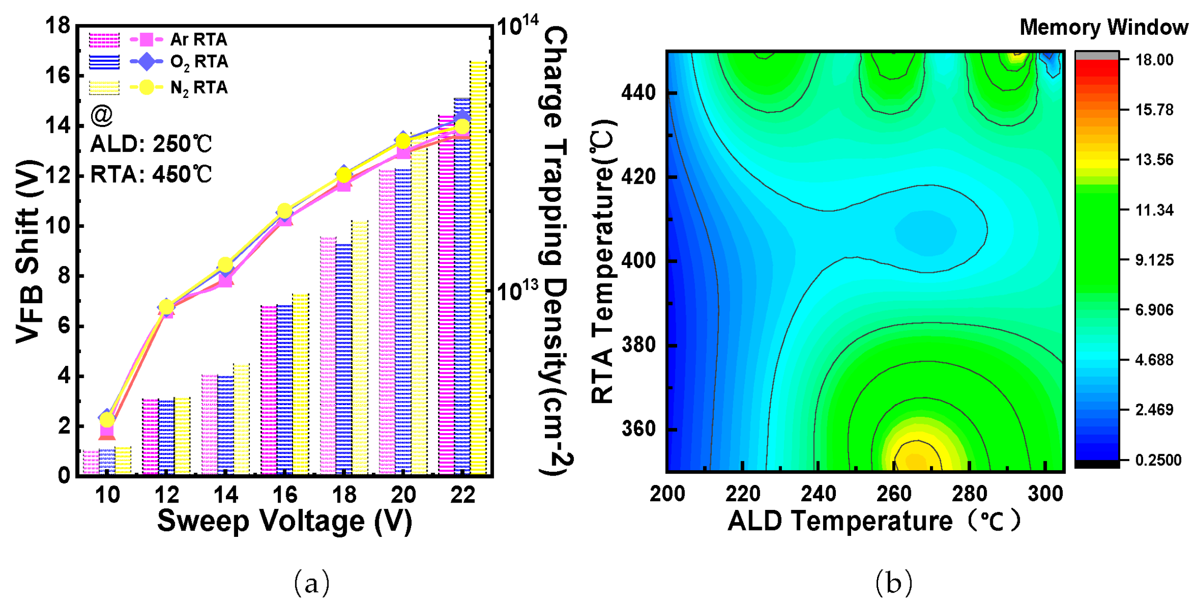
2.1. Experiment Methods

Al/Al₂O₃/HfAlO/Al₂O₃/Si-structured NVM devices were prepared using (1–10 Ω·cm) p-type Si as substrate and crystal orientation is (100). The structure of the device is shown in Figure 3a, where the tunneling layer is 3 nm Al₂O₃ (to control the tunneling effect of the charge in the dielectric layer) and the blocking layer is 20 nm Al₂O₃ (for limiting the diffusion of the charge in the dielectric layer). The wafers were first cleaned by using the RCA standard cleaning method, then the deposition cycle of the ALD (Atomic Layer Deposition) system was used to prepare approximately 3 nm Al₂O₃ (at different temperatures) as the tunneling layer. The deposition cycle of ALD was then adjusted to obtain different thicknesses of HfO₂ and Al₂O₃ overlays as trapping layers and to control the overall thickness to 18 nm. After completion of oxide deposition, the devices were annealed for different lengths of time using rapid thermal annealing (RTA) at different temperatures under N₂/O₂/Ar conditions, respectively. Finally, 300 nm thick Al was deposited on the blocking layer using thermal evaporation. The memory characteristics of the charge trapping memory were obtained using the capacitance–voltage test, and the memory window of the device was obtained according to Figure 3b–e. The experiment was then repeated, using different voltages and temperatures for the devices to obtain 156 data sets.

2.2. Data Pre-Processing

In order to improve the comparability between data and convergence speed and shorten the training time, the original data were normalized and compressed to the interval of [0, 1]. The Min-Max Normalization (MMSN) was used:

$$x_{norm}=\frac{x-x_{min}}{x_{max}-x_{min}}$$

(1)

where x and x_norm are the original data and the normalized data, respectively; x_max and x_min are the maximum and minimum values of the data, respectively. For the gas type variables, the different gases N₂, O₂, and Ar are defined as 0, 1, and 2, respectively.

2.3. Optimization Methods

The dataset was divided into an 80% training dataset and a 20% test dataset, then imported into the pre-constructed SVR model. To optimize the model parameters of SVR, six different swarm algorithms were utilized. The optimization process, known as SI-SVR, is depicted in Figure 4. In this study, we employed the Python package “mealpy” to construct the swarm intelligence SVR model [13]. Python source code for all meta-inspired SVR algorithms presented in this paper is openly accessible on GitHub at the following link: https://github.com/MONKEYHUYIFAN/SISVR_memorydevice (accessed on 30 May 2023).

2.3.1. Whale Optimization Algorithm (WOA)

The Whale Optimization Algorithm (WOA) is a nature-inspired method of optimization, proposed by Mirjalili et al., in 2016 [14]. The algorithm mimics the hunting behavior of humpback whales and employs a population divided into three groups to effectively explore and exploit the search space. WOA offers several advantages, including its simplicity, requiring minimal control parameters, and achieving a fine balance between exploration and exploitation. Additionally, it is applicable to a wide range of optimization problems without relying on problem-specific knowledge. However, the performance of WOA is heavily influenced by the initial population and control parameters, which highlights the importance of proper parameter tuning. Moreover, WOA may encounter challenges when dealing with high-dimensional problems. Therefore, the selection of suitable techniques and careful parameter tuning are crucial for addressing these challenges and maximizing the algorithm’s performance.

2.3.2. Pelican Optimization Algorithm (POA)

The Pelican Optimization Algorithm (POA) is a nature-inspired optimization algorithm that mimics the foraging behavior of pelicans. In this algorithm, candidate solutions are represented by virtual pelicans, and a population-based approach is employed. The algorithm integrates both exploration and exploitation strategies with the objective of efficiently searching for the optimal solution. Drawing inspiration from the flocking behavior and competitive dynamics observed in pelicans, the algorithm facilitates information sharing among individuals while they compete for superior prey, which corresponds to favorable solutions in the optimization context. The POA has exhibited promising results when applied to diverse optimization problems, establishing an effective balance between exploration and exploitation, and enabling a thorough and effective search for solutions [15].

2.3.3. Grey Wolf Optimization (GWO)

The Grey Wolf Optimization (GWO) is a nature-inspired algorithm that initiates with a randomized population of grey wolves, which represent candidate solutions. These wolves are organized into groups, and their distances to the target prey are measured. During the search process, each wolf undergoes updates utilizing robust operations, guided by two parameters that strike a balance between exploration and exploitation, thereby mitigating the risk of getting trapped in local optima. Distinguishing itself from other population-based algorithms, the GWO’s mathematical model facilitates the relocation of a solution around another solution within an n-dimensional search space, closely simulating the hunting behavior of grey wolves. Notably, GWO requires less memory compared to Particle Swarm Optimization (PSO) and only retains three optimal solutions. Its unique equations have contributed to its rapid growth within the field of swarm intelligence algorithms. GWO has demonstrated successful applications across diverse optimization problems, encompassing global optimization, power engineering, scheduling, control engineering, robotics, and environmental planning [16].

2.3.4. Moth-Flame Optimization (MFO)

The Moth Flame Optimization (MFO) algorithm utilizes a predefined number of moths to explore the solution space in search of optimal locations that align with the objective function. The movement of the moths is determined by an update formula that guides their wandering routes. Within the population of moths, the flame represents the best solution discovered thus far, and it can vary in number. This adaptive selection of flames guarantees ongoing improvement throughout the optimization process, as the moths converge towards more favorable solutions [17].

2.3.5. Particle Swarm Optimization (PSO)

The particle swarm algorithm originated from a study of the foraging behavior of bird flocks and was introduced by J. Kennedy et al., in 1995 [18]. In this algorithm, a group of birds collectively explores the search space in order to find the optimal destination by sharing information. A flock of birds ventures into a forest in search of food, aiming to locate the area with the highest food abundance. Although lacking precise knowledge of the food’s exact location, each bird possesses a general sense of the approximate direction. Individually, the birds navigate their chosen paths, recording the location with the greatest food yield and its corresponding quantity. As the search progresses, each bird adjusts its direction based on the best food source it has encountered and the collective discoveries of the entire flock. Over time, through this collaborative effort, the flock gradually converges on the location within the forest that offers the maximum food resources, representing the global optimal solution.

2.3.6. Osprey Optimization Algorithm (OOA)

In 2023, Pavel Trojovsky et al. [19] introduced an optimization algorithm that draws inspiration from the hunting behavior of osprey. This algorithm emulates the strategies employed by ospreys during their hunting process, exhibiting remarkable optimization capabilities and rapid convergence. By leveraging the inherent characteristics of ospreys, the proposed algorithm demonstrates a strong aptitude for efficiently locating optimal solutions.

2.4. Model Error Detection

Model fit accuracy is commonly assessed through graphical representation of predicted and true values. However, this method lacks precision in measuring differences and is primarily useful for identifying trends. To effectively compare model performance, various metrics can be used, such as mean squared error (MSE), coefficient of determination (R²), deviation between predicted and true values, and mean absolute percentage error (MAPE). MSE quantifies bias, with smaller values indicating better fit, while R² reveals the proportion of input variables explaining output variables, with larger values indicating improved fit. Additionally, the MAPE calculates the average error relative to the true value, with smaller values suggesting a better fit. To evaluate the generalization of the model and prevent overfitting, cross-validation is a valuable technique. K-fold cross-validation is a popular method that entails dividing the dataset into “k” groups. Each group serves as a validation set while the model is trained on the remaining “k − 1” groups. This process is repeated “k” times to ensure that every group is used for validation once. By calculating the average error across all trials, a more robust measure of model performance can be obtained.

These methods provide a comprehensive assessment of model fit and generalization, allowing for more accurate comparisons between models. Figure 5 further demonstrates the rationale for cross-validation. A five-fold cross-validation was used in this study, and the average correlation coefficient of the cross-validation is referred to as the MCV score.

3. Results and Discussions

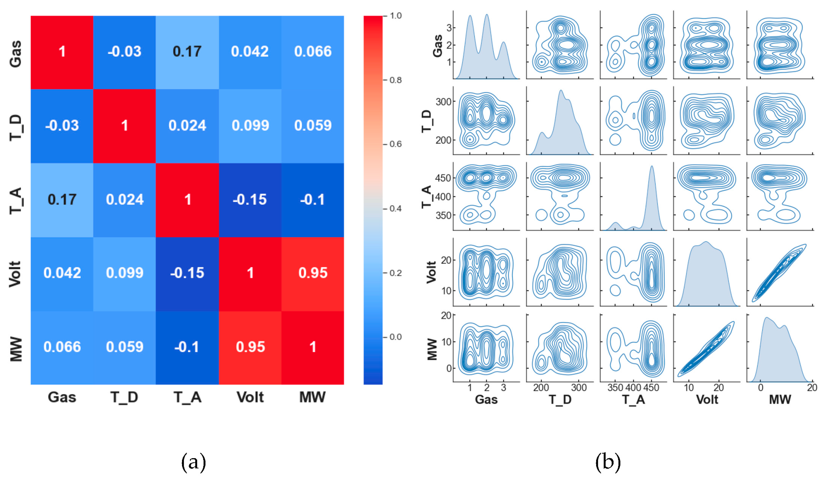
3.1. Dataset Pre-Analysis

Using the experimental dataset obtained in Section 2.1, which includes four input variables (gas type, rapid thermal annealing process temperature, ALD preparation temperature, and sweep voltage) and one output variable (memory window), a total of 156 data samples were selected. The statistical analysis presented in Figure 6a shows that although there is no obvious positive linear correlation between these five categories of data, the process conditions clearly affect the memory window characteristics of the device. It can be seen in Figure 6b that the high storage property results in higher frequency under some specific conditions, which is reflected in the kernel density plot as more dense data in a certain region. Therefore, it is critical to predict the optimal process conditions. Only the variable voltage has a more obvious positive correlation property with the memory window, so it is necessary to use the SVR model to investigate the relationship between other variables and the memory window.

Figure 7b shows the increase in charge trapping density and memory window with increasing scan voltage when thermal annealing is performed under different gases. When the ALD and RTA temperatures were determined to be 250 °C and 450 °C, the results of annealing under N₂ atmosphere were better (more than 16 V), which confirms the positive correlation between scan voltage and memory window in Figure 6a. The memory window at different RTA and ALD temperatures is shown in Figure 7b. It shows the two process temperatures while tuning the size of the memory window; in several areas, the extreme value of the memory window can be seen, which demonstrates that the effect of process temperature on the memory window is very unstable.

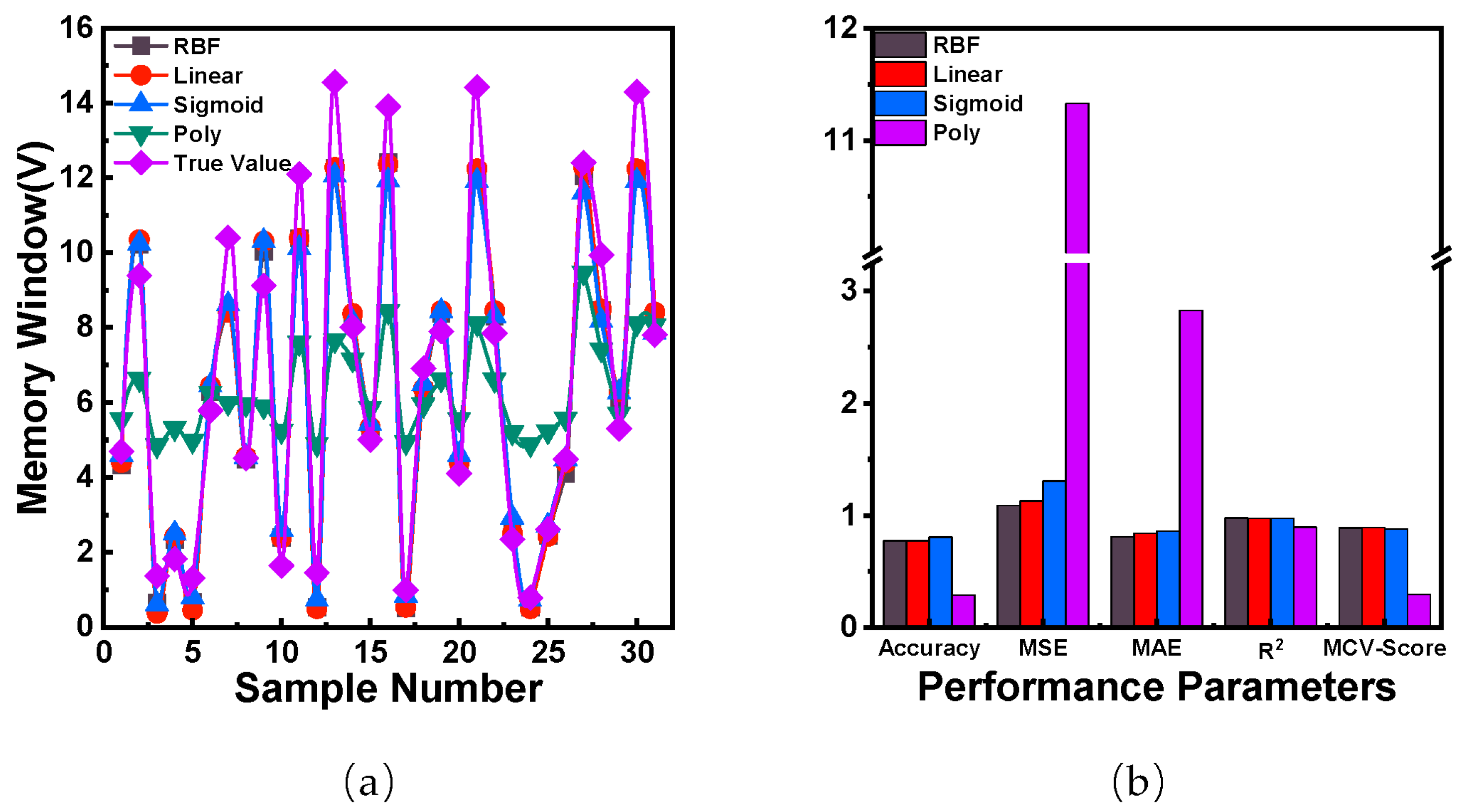
3.2. Comparison of Different Kernel Function

The selection of appropriate kernel functions is crucial when employing support vector regression for prediction purposes. In this study, various kernel functions, including Radial Basis Function (rbf), Sigmoid, Linear, and Polynomial functions (Poly), are utilized within the SVR model. To assess the model’s performance, the training set was employed for training with different kernel functions. Subsequently, the validation set was used for testing, and the corresponding results are depicted in the figure below.

It can be seen from Figure 8a that the prediction accuracy of the poly kernel function is the lowest because it is highly prone to overfitting, leading to large errors due to its high complexity, and is determined by the order values. The other kernel functions had similar fitting effects. Therefore, we calculated their error parameters. The linear kernel function performed better in all areas because the linear kernel function is usually used for linearly separable data and the data set itself is small and contains some linear relationships; therefore, it performed better in this case. However, the sigmoid function was used under too harsh conditions and thus produced large MSE and MAE in this model; in such cases, the radial basis function has better values. Because RBF is not limited by the spatial dimension and sample size, it is suitable for fitting small data sets. The relevant specific data have been listed in

Table 1. Comparison of performance metrics of different kernel functions.

Model	Accuracy *(%)	MSE	MAE	R2	MCV-Score
Linear	77.4	1.13	0.84	0.975	0.899
Sigmoid	80.6	1.31	0.86	0.975	0.880
RBF	87.1	0.55	0.58	0.987	0.876
Poly	80.6	0.59	0.58	0.987	0.858

* The accuracy is defined as the ratio of data that differs from the actual value by less than 10% to test database.

. The comprehensive table data shows that, although sigmoid achieved 80.6% recognition accuracy, it performed poorly in other metrics, which may be due to the chance of the dataset. The RBF is widely applicable and performs well in general SVR experiments, so this model used the RBF kernel function for the next experiments.

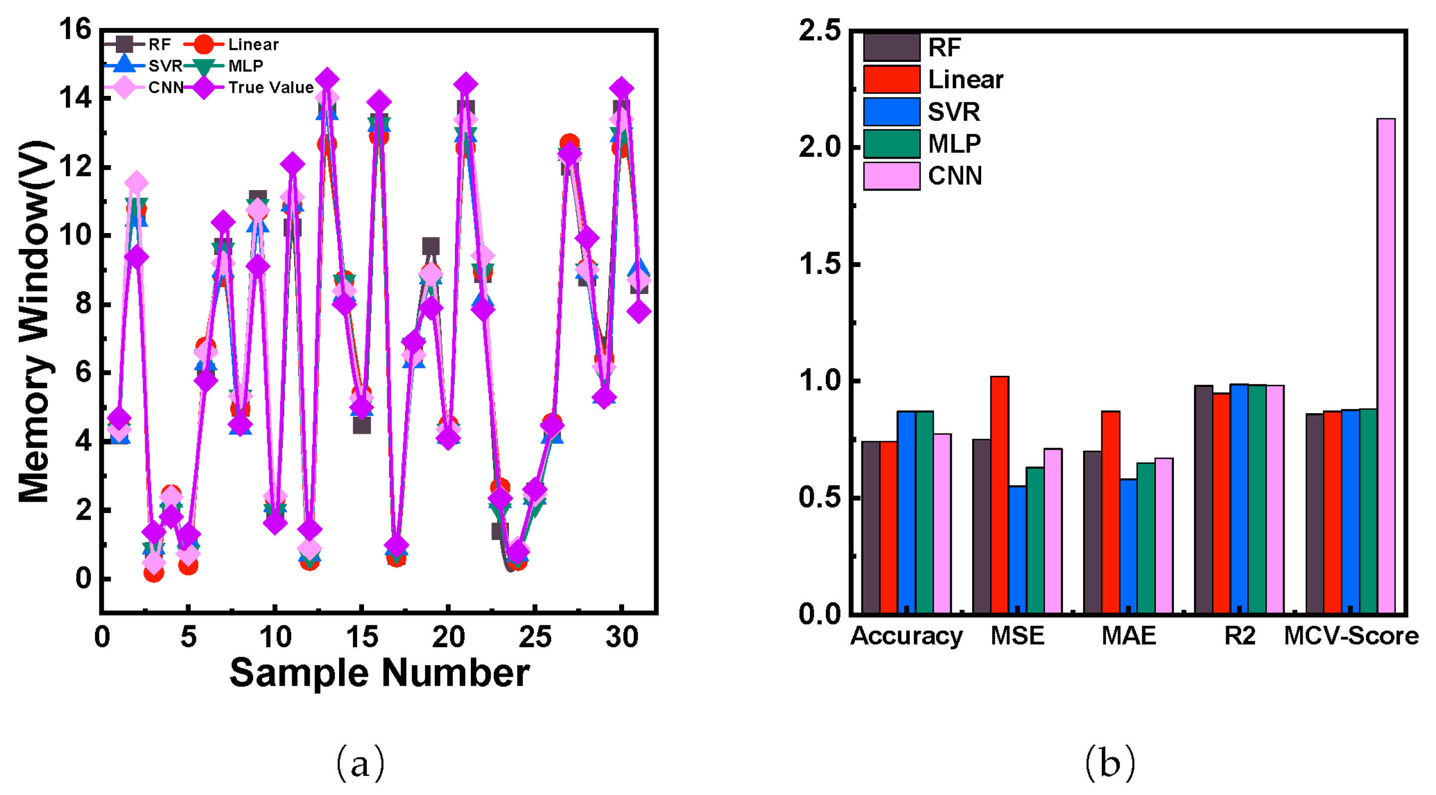
3.3. Comparison with Other Models

The dataset was also modelled and forecasted using Multiple Linear Regression (MLR), Random Forest (RF) techniques with Multi-Layer Perceptron (MLP) neural network models, and CNN (Convolutional Neural Networks), and their model assessment metrics were compared with the SVR model utilizing RBF kernel functions. As shown in Figure 9a, the prediction results of the real values and the three models of SVR and BP neural networks are shown on the same plane. It can be found that the trends of the predicted values of these models are basically the same as those of the real values. The difference is that the predicted value of SVR is closer to the true value, which is better than the predicted value of RF and linear model. SVR and MLP achieved 87.1% prediction accuracy, and the SVR model performed very well in MSE and MAE, achieving 0.55 and 0.58, respectively, which were much lower than the other four models. The reason for the poor performance of CNN algorithms compared to MLP algorithms is that CNNs are primarily designed to work with image data, and they can effectively deal with spatial relationships between pixels using convolutional layers. However, for tabular data, such spatial relationships do not exist and hence using CNNs cannot provide better results than other models. The data also proves that Random Forest, Support Vector Machines, and MLP will provide better results when dealing with tabular data. The SVR model achieved an R² of 0.987 and an MCV score of 0.876, which are better than other models. The final solution of SVR is theoretically optimal in terms of nonlinear fitting to a high-dimensional feature space, solving the local extremum problem that cannot be avoided in neural network methods [20], all the performance metrics are shown in

Table 2. Comparison of performance metrics for different prediction models.

Model	Accuracy (%)	MSE	MAE	R2	MCV-Score
SVR	87.1	0.55	0.58	0.987	0.876
RF	74.2	0.75	0.7	0.980	0.859
MLP	87.1	0.63	0.65	0.984	0.881
CNN	77.4	0.71	0.67	0.982	2.123
MLR	74.2	1.02	0.87	0.947	0.871

.

3.4. Different Swarm Algorithm Optimization

In SVR, finding both the kernel function parameter and optimal penalty parameter C and epsilon is a typical global optimization problem. To further improve the accuracy of the support vector regression prediction model, we introduce several swarm intelligence algorithms, including GWO, WOA, OOA, POA, MFO, and PSO. To optimize the parameters of SVR, especially the epsilon and penalty parameter C. For example, the global search property of GWO gives it the ability to find a better combination of parameters, and it does not require information about the derivatives of the objective function, which allows it to be applied to complex nonlinear optimization problems. The implementation of the GWO is relatively simple, with fewer algorithm parameters, which makes it easy to understand and implement. For optimization problems with SVR parameters, the range of parameters, population size, and number of iterations can be easily adjusted using the grey wolf algorithm to meet the needs of a particular problem. We wrote six different swarm intelligence codes using Python and imported the dataset to find the result that makes the highest average cross-verification score. We also compared the predicted values with the true values of the test dataset, as shown in Figure 10.

In this optimization, the initial parameters of the optimization algorithm were adjusted through a large number of pre-tests, the number of feasible solutions was established to 30, the maximum value of iterations was subjected to 150, the upper and lower limits of the penalty parameter C and the kernel function were set to [0.01, 100] and [0.001, 10], respectively, the optimal epsilon and penalty parameter C were calculated and applied to the traditional nonlinear SVR, and then the training set data were used to train the SVR. The SVR was trained, and then the test set was used to calculate MSE, MAE, MAPE, R², accuracy, etc., to obtain the prediction effects of each algorithm, as shown in

Table 3. Summary of errors of different swarm intelligence optimization methods.

Model	Accuracy (%)	MSE	MAE	R2	MCV-Score	Epsilon	C
SVR	87.1	0.55	0.58	0.987	0.876	0.01	10
MFO	90.3	0.64	0.63	0.98445	0.88349	0.26495	31.66204
GWO	90.3	0.64	0.63	0.98856	0.88349	0.26479	31.52233
POA	90.3	0.64	0.63	0.98445	0.87317	0.265	31.62074
WOA	90.3	0.65	0.63	0.98419	0.88332	0.27517	29.11249
PSO	90.3	0.64	0.63	0.98446	0.87666	0.26474	31.52349
OOA	90.3	0.64	0.63	0.98447	0.88350	0.26473	31.4981

, and the five-fold cross-validation of different models was performed, before finally the test set was used as the effect validation data to obtain the five-fold cross-validation values of the model evaluation metrics (MSE, 𝑅², and MAPE). The specific effect is shown in Figure 11a. As shown in Figure 11a, all model predictions differ very little from the true values and almost overlap. To compare the prediction effects of these five types of models, the error performance parameters of the model are shown in Figure 11b. The specific values are shown in the following Table 3.

As presented in Table 3, all the optimization algorithms exhibited comparable prediction accuracy in terms of MSE and MAE. However, the MFO, GWO, POA, and OOA algorithms outperformed the other two algorithms in terms of R² and cross-verification scores, as evident from the optimization results. Compared to the SVR model without an optimization algorithm, the inclusion of an optimization algorithm resulted in a 3.2% increase in recognition accuracy at a 20% recognition error tolerance rate. The optimized model showed a slight increase in MSE and MAE due to the introduction of new Epsilon and C values by the optimization algorithm. The MCV scores, which demonstrate the overall adaptability of the model, indicated a notable improvement of 0.0075. Additionally, there was an improvement of 0.00156 in R². The code kernels of these clustering algorithms are similar and have fewer differences; therefore, the C and Epsilon obtained are closer and have fewer differences, whereas SVR without the clustering algorithms uses the default C and Epsilon from the sklearn library, and therefore does not perform as well as the SVR with clustering algorithms. These findings indicate that the optimized SVR model possesses strong predictive power, performs well on different subsets, exhibits good generalization ability, and may yield better performance on unseen data. The optimized model also demonstrates relative stability against data volatility and noise, reducing the risk of overfitting to specific datasets. In terms of running speed and total time cost, a comparison of different optimization algorithms was conducted, as shown in Figure 11a,b. While an ideal and effective search method would involve iterating all SVR parameters in fixed steps and comparing the results, this approach is time-consuming. After testing, it was found that a cycle takes approximately 0.5 s to complete when using an iterative program, with the upper and lower limits of the iterative process set to (1, 100) for C with a step size of 0.1, and (0.01, 10) for Epsilon with a step size of 0.01. The program takes approximately 5 × 10⁵ s to complete. Therefore, a simpler optimization algorithm is necessary to reduce the optimization time. The computational resources and time required by the algorithms depend on various factors. The PSO, WOA, MFO, and GWO algorithms demonstrated faster execution under this dataset, partly due to their relatively simple search strategies and update rules. It should be noted that different optimization problems may respond differently to different algorithms, and the selected algorithms were able to find the optimal solution more efficiently for the small dataset in this study. However, all the optimization algorithms significantly improved the efficiency of the exhaustive enumeration method by a factor of 2660 to 5893 times, resulting in a substantial reduction in the optimization search time.

In addition to iteration speed, the efficiency of the fitness function is also of great importance. Figure 12 shows that all algorithms, except for the WOA optimization algorithm, reached convergence within approximately 20 iterations, while the WOA algorithm took around 50 iterations to converge. It is worth noting that all algorithms achieved convergence within 50 iterations and improved the fitness by more than 0.001. Considering the overall performance of all the models, in this study with a small dataset size and dense distribution of feature variables, the MFO and GWO algorithms demonstrated the best performance among all the algorithms. These algorithms not only provided more accurate prediction results but also exhibited higher cross-validation scores, indicating their strong stability. Furthermore, both MFO and GWO algorithms demonstrated a higher iteration speed compared to the other algorithms, significantly reducing the optimization search time.

4. Conclusions

This study focuses on the optimization of process parameters for HfAlO-based charge trapping memory devices using the SI-SVR model. The SVR model was optimized using six different swarm algorithms, and the optimized SVR model achieved high accuracy and stability in the experimentally obtained dataset with a mean squared error of 0.64, mean absolute error of 0.63, R² of 0.98856, recognition accuracy of 90.3%, and MCV score of 0. 88350, and it was found that the GWO algorithm and MFO algorithms performed well on this dataset. Higher search efficiency and convergence speed were achieved. The results demonstrate the effectiveness of using machine learning for process optimization in non-volatile memory manufacturing. This study provides valuable insights for improving the performance of non-volatile memories.

References

1. Research, G.V. Next Generation Non Volatile Memory Market Size, Share & Trends Analysis Report by Product (FeRAM, PCM, MRAM, ReRAM), by Application, by Region, and Segment Forecasts, 2018–2024. In Market Analysis Report; Grand View Research: Pune, India, 2015. [Google Scholar]
2. Nowak, E.; Chłopocka, E.; Szybowicz, M. ZnO and ZnO-Based Materials as Active Layer in Resistive Random-Access Memory (RRAM). Crystals 2023, 13, 416. [Google Scholar] [CrossRef]
3. Hu, Y.; Rabelo, M.; Kim, T.; Cho, J.; Choi, J.; Fan, X.; Yi, J. Ferroelectricity Based Memory Devices: New-Generation of Materials and Applications. Trans. Electr. Electron. Mater. 2023, 24, 271–278. [Google Scholar] [CrossRef]
4. Redaelli, A.; Petroni, E.; Annunziata, R. Material and Process Engineering Challenges in Ge-Rich GST for Embedded PCM. J. Mater. Sci. Semicond. Process. 2022, 137, 106184. [Google Scholar] [CrossRef]
5. Alahmadi, A.; Chung, T.S. Crash Recovery Techniques for Flash Storage Devices Leveraging Flash Translation Layer: A Review. Electronics 2023, 12, 1422. [Google Scholar] [CrossRef]
6. Shen, S.C.; Khare, E.; Lee, N.A.; Saad, M.K.; Kaplan, D.L.; Buehler, M.J. Computational Design and Manufacturing of Sustainable Materials through First-Principles and Materiomics. Chem. Rev. 2023, 123, 2242–2275. [Google Scholar] [CrossRef] [PubMed]
7. Yoo, J.-H.; Park, W.-J.; Kim, S.-W.; Lee, G.-R.; Kim, J.-H.; Lee, J.-H.; Uhm, S.-H.; Lee, H.-C. Preparation of Remote Plasma Atomic Layer-Deposited HfO2 Thin Films with High Charge Trapping Densities and Their Application in Nonvolatile Memory Devices. Nanomaterials 2023, 13, 1785. [Google Scholar] [CrossRef] [PubMed]
8. D’Acunto, G.; Tsyshevsky, R.; Shayesteh, P.; Gallet, J.-J.; Bournel, F.; Rochet, F.; Pinsard, I.; Timm, R.; Head, A.R.; Kuklja, M.; et al. Bimolecular Reaction Mechanism in the Amido Complex-Based Atomic Layer Deposition of HfO2. Chem. Mater. 2023, 35, 529–538. [Google Scholar] [CrossRef] [PubMed]
9. Goh, G.D.; Lee, J.M.; Goh, G.L.; Huang, X.; Lee, S.; Yeong, W.Y. Machine Learning for Bioelectronics on Wearable and Implantable Devices: Challenges and Potential. Tissue Eng. Part A 2022, 29, 20–46. [Google Scholar] [CrossRef] [PubMed]
10. Pradeep, D.; Vardhan, B.V.; Raiak, S.; Muniraj, I.; Elumalai, K.; Chinnadurai, S. Optimal Predictive Maintenance Technique for Manufacturing Semiconductors using Machine Learning. In Proceedings of the 2023 3rd International Conference on Intelligent Communication and Computational Techniques (ICCT), Jaipur, India, 19–20 January 2023; pp. 1–5. [Google Scholar]
11. Szczepaniuk, H.; Szczepaniuk, E.K. Applications of Artificial Intelligence Algorithms in the Energy Sector. Energies 2023, 16, 347. [Google Scholar] [CrossRef]
12. Bradshaw, T.J.; Huemann, Z.; Hu, J.; Rahmim, A. A Guide to Cross-Validation for Artificial Intelligence in Medical Imaging. Radiol. Artif. Intell. 2023, 5, e220232. [Google Scholar] [CrossRef]
13. Van Thieu, N.; Mirjalili, S. MEALPY: An Open-Source Library for Latest Meta-Heuristic Algorithms in Python. J. Syst. Archit. 2023, 139, 102871. [Google Scholar] [CrossRef]
14. Mirjalili, S.; Lewis, A. The Whale Optimization Algorithm. Adv. Eng. Softw. 2016, 95, 51–67. [Google Scholar] [CrossRef]
15. Trojovský, P.; Dehghani, M.J.S. Pelican optimization algorithm: A novel nature-inspired algorithm for engineering applications. Sensors 2022, 22, 855. [Google Scholar] [CrossRef] [PubMed]
16. Mirjalili, S.; Mirjalili, S.M.; Lewis, A. Grey Wolf Optimizer. Adv. Eng. Softw. 2014, 69, 46–61. [Google Scholar] [CrossRef] [Green Version]
17. Mirjalili, S. Moth-Flame Optimization Algorithm: A Novel Nature-Inspired Heuristic Paradigm. J. Knowl.-Based Syst. 2015, 89, 228–249. [Google Scholar] [CrossRef]
18. Kennedy, J.; Eberhart, R. Particle Swarm Optimization. In Proceedings of the ICNN’95—International Conference on Neural Networks, Perth, WA, Australia, 27 November–1 December 1995; IEEE: Piscataway, NJ, USA, 1995; pp. 1942–1948. [Google Scholar]
19. Trojovský, P.; Dehghani, M. Osprey Optimization Algorithm: A New Bio-Inspired Metaheuristic Algorithm for Solving Engineering Optimization Problems. J. Front. Mech. Eng. 2023, 8, 136. [Google Scholar]
20. Huang, S.; Tian, L.; Zhang, J.; Chai, X.; Wang, H.; Zhang, H. Support Vector Regression Based on the Particle Swarm Optimization Algorithm for Tight Oil Recovery Prediction. ACS Omega 2021, 6, 32142–32150. [Google Scholar] [CrossRef] [PubMed]
Figure 1. Non-volatile memory world market trend [1].
Electronics 12 03139 g001
Figure 2. Schematic diagram of support vector regression.
Electronics 12 03139 g002
Figure 3. (a) MOS device structure in the dataset; (b) C–V curve under different voltage @ 450 °C N2 RTA and 250 °C ALD; (c) C–V curve under different ALD temperature @ 450 °C N2 RTA and 20 V voltage; (d) C–V curve under different gas @ 450 °C RTA, 250 °C ALD and 20 V voltage; (e) C–V curve under different ALD temperature @ 450 °C N2 RTA and 20 V voltage.
Electronics 12 03139 g003
Figure 4. Flow chart of HfAlO device memory window prediction.
Electronics 12 03139 g004
Figure 5. Schematic diagram of cross-validation.
Electronics 12 03139 g005
Figure 6. (a) Heat map of dataset; (b) pairplot of independent and dependent variables.
Electronics 12 03139 g006
Figure 7. (a) Memory window under specific conditions; (b) Contour maps of deposit versus thermal annealing temperature and memory window.
Electronics 12 03139 g007
Figure 8. (a) Comparison of prediction value and true value by using different kernel function; (b) Model error performance parameters.
Electronics 12 03139 g008
Figure 9. (a) Comparison of prediction value and true value by using different models; (b) Model error performance parameters.
Electronics 12 03139 g009
Figure 10. (a) Comparison of prediction value and true value by using swarm algorithm; (b) Model error performance parameters.
Electronics 12 03139 g010
Figure 11. (a) Average speed of different algorithms at different iterations; (b) Optimization total algorithm time cost.
Electronics 12 03139 g011
Figure 12. Iterative process of different swarm algorithms.
Electronics 12 03139 g012