Development of Building Thermal Load and Discomfort Degree Hour Prediction Models Using Data Mining Approaches


1
School of Civil Engineering and Architecture, Wuhan University of Technology, Wuhan 430070, China
2
College of Engineering and Science, Victoria University, Melbourne 8001, Australia
3
School of Engineering, RMIT University, Melbourne 3000, Australia
*
Author to whom correspondence should be addressed.
Energies 2018, 11(6), 1570; https://doi.org/10.3390/en11061570
Submission received: 26 May 2018
/
Revised: 12 June 2018
/
Accepted: 14 June 2018
/
Published: 14 June 2018
(This article belongs to the Special Issue Energy Efficiency in Plants and Buildings 2019)
Abstract
:Thermal load and indoor comfort level are two important building performance indicators, rapid predictions of which can help significantly reduce the computation time during design optimization. In this paper, a three-step approach is used to develop and evaluate prediction models. Firstly, the Latin Hypercube Sampling Method (LHSM) is used to generate a representative 19-dimensional design database and DesignBuilder is then used to obtain the thermal load and discomfort degree hours through simulation. Secondly, samples from the database are used to develop and validate seven prediction models, using data mining approaches including multilinear regression (MLR), chi-square automatic interaction detector (CHAID), exhaustive CHAID (ECHAID), back-propagation neural network (BPNN), radial basis function network (RBFN), classification and regression trees (CART), and support vector machines (SVM). It is found that the MLR and BPNN models outperform the others in the prediction of thermal load with average absolute error of less than 1.19%, and the BPNN model is the best at predicting discomfort degree hour with 0.62% average absolute error. Finally, two hybrid models—MLR (MLR + BPNN) and MLR-BPNN—are developed. The MLR-BPNN models are found to be the best prediction models, with average absolute error of 0.82% in thermal load and 0.59% in discomfort degree hour.
1. Introduction
Building design optimization involves the integration of an optimization algorithm with building performance calculation. Oftentimes the building performance calculation conducted by simulation software is time-consuming; therefore, the development of performance prediction models is a good alternative to significantly reduce the computation time.
Annual thermal load and indoor comfort level are two important factors in evaluating the performance of buildings and they are often the objectives of building design optimization [1,2,3,4,5,6,7]. For example, Gong et al. [2] applied the orthogonal method and the listing method to optimize passive building design to minimize the annual thermal load. Yu et al. [3] applied a multiobjective genetic algorithm to optimize building energy efficiency and thermal comfort.
Insulation thickness, concrete slab thickness, window-to-wall ratio (WWR), and optical properties of the envelope (absorption/reflection of solar) are critical factors that affect the building performance and have attracted the interest of many researchers [6,8,9]. For example, Yuan et al. [6] presented a proposal to find an optimal combination of reflectivity and insulation thickness of building exterior walls to minimize the annual thermal load and cost of the building envelope. Wang et al. [8] investigated the optimal slab thickness of the building envelope to maintain the indoor air temperature within a prescribed temperature range without turning on the heating, ventilation and air-conditioning (HVAC) system. A concrete slab thickness of 25 cm was recommended for the ceiling and floor and 10 cm for the envelope wall. The maximum WWR was then given as a function of diurnal temperature amplitude. Olivieri et al. [9] performed an experimental study to find the optimal insulation thickness of a vertical green wall under the continental Mediterranean climate and found an insulation thickness of 9 cm to be sufficient.
Building simulation software, such as TRNSYS [1], THERB [2], EnergyPlus [4], and New HASP/ACLD-β [6] have been used to obtain the thermal load and/or indoor thermal comfort condition. Such programs require dynamic computing to calculate the hourly/subhourly thermal load and indoor comfort condition. It becomes time-consuming when providing annual results, especially when coupled with an optimization algorithm and many iterations are inevitable in order to find the optimum building design solutions.
Data mining techniques can be used to develop prediction models based on experimental or simulation datasets to replace extensive simulation efforts, so as to reduce the computation time to evaluate the building performance indices. For instance, artificial neural network (ANN) models have been developed to predict the annual building energy consumption/thermal comfort condition to reduce the computation time during the optimization process [1,3,5].
Prediction models based on data mining techniques have been verified to have good performance in the prediction of heating and cooling load [10], building energy demand [11], electricity demand [12,13], and energy consumption [14,15,16]. For example, Tsanas and Xifara [10] used statistical machine learning tools to predict the building heating load and cooling load with low mean absolute error deviations of 0.51 and 1.42 using a random forest (RF) approach, compared with the results from Ecotech. Yu et al. [11] developed a decision tree method to predict building energy demand with 93% accuracy for training data and 92% accuracy for test data. Wang et al. [12] developed an ‘Ensemble Bagging Trees’ (EBT) technique using data obtained from meteorological systems and building-level occupancy and meter to predict the hourly electricity demand of a test building with Mean Absolute Prediction Error ranging from 2.97 to 4.63%.
Some researchers have employed different approaches and compared the outcomes of prediction from various models [17,18,19,20,21]. Those models are developed for predictions of hourly energy usages [17], steam load [18], energy consumption [19,20], cooling load, and heating load [21]. For instance, Chou and Bui [21] utilized support vector regression (SVR), ANN, classification and regression tree (CART), chi-squared automatic interaction detector, general linear regression, and ensemble inference models to predict the energy performance of buildings and found that the ensemble approach (SVR + ANN) and SVR were the best models for predicting cooling load and heating load, with mean absolute percentage errors of 3.46% and 1.13%, respectively. Ahmad et al. [19] compared the performance of RF and ANN in the prediction of building energy consumption and found that ANN performed marginally better than RF.
It can be foreseen that a data mining approach can also be applied to predict annual thermal load and indoor thermal comfort conditions with satisfactory performance. Therefore, in this paper, seven data mining techniques, including multilinear regression (MLR), Chi-square Automatic Interaction Detector (CHAID), Exhaustive CHAID (ECHAID), back-propagation neural network (BPNN), radial basis function network (RBFN), CART, and support vector machines (SVM), are used to develop prediction models for annual building thermal load and discomfort degree hours and their performances are evaluated. Finally, two hybrid models, called MLR (MLR + BPNN) and MLR-BPNN models, are developed to improve the prediction accuracy.
2. Database Construction
2.1. Base Building Model
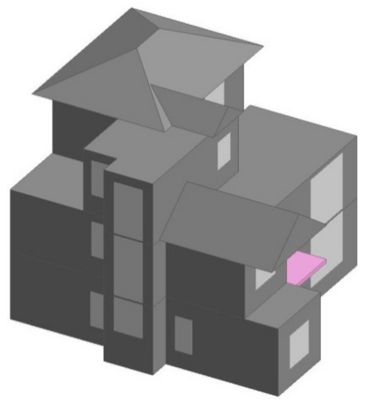
A three-story residential building (see Figure 1) with floor area of 146.43 m2, total construction area of 303.9 m2, and height of 11.77 m was selected for study. It is located in Wuhan city, which is a representative city that belongs to the hot summer and cold winter region in China. Most of the cities in this region are in the middle and lower reaches of the Yangtze River, and are all located in the north of the Tropic of Cancer. The buildings in this region are mainly oriented towards the south in order to obtain more solar radiation in winter. According to the residential building energy efficiency design standard for the hot summer/cold winter region JGJ134-2010 [22], the optimal building orientation in Wuhan city is 15° South to West, which is applied in this study.
Natural ventilation is adopted to use free cooling to reduce the thermal load. The infiltration rate is 0.5 air change rate per hour (ACH) according to the building energy efficiency standard [22]. There is an overhang at the entrance of the building to provide shading. Low-E glazing is selected to ensure enough daylighting while effectively reducing the unwanted solar radiation in the daytime, and the roof overhangs act as shading devices for the windows. Internal shading devices can be used when needed.
The occupancy level is 50 m2/person, and the infiltration rate is 0.5 ACH, which is also the minimum fresh air rate required by GB 50736-2012 [23]. The metabolic factor is 0.87 (Men = 1.0, women = 0.85, children = 0.75), representing two adult men, two adult women, and two children. The clothing level is 1.0 clo. in winter and 0.5 clo. in summer [24]. The heating temperature setpoint is 18 °C with a setback temperature of 16 °C and the cooling temperature setpoint is 26 °C with a setback temperature of 28 °C, according to JGJ134-2010 [22]. Natural ventilation is ON with a maximum ventilation rate of 3 ACH by zone control to reduce the building thermal load. A heat pump is selected to provide cooling in summer and heating in winter. The HVAC system is ON when occupied.
2.2. Independent and Dependent Variables
2.2.1. Independent Variables
Double-layer Low-E windows are installed on each side of the building. The layer-to-layer information for the roof is as follows (from exterior to interior): asphalt waterproof layer, extruded polystyrene board (XPS) insulation layer, concrete layer, and lime-and-cement mortar layer. No skylight is assumed. The structures of the exterior walls are as follows: face brick layer, XPS insulation layer, concrete layer, and lime-and-cement mortar layer. WWR, absorptance of solar radiation at the outer layer surface, insulation thickness, and concrete thickness are identified as the four groups of parameters that have an important impact on the building thermal performance due to the following reasons [24]: (1) Thermal mass can affect the fluctuation of the daily temperature inside the house. (2) Insulation can affect the conduction heat gain/loss through the opaque envelope. (3) The absorptance of solar radiation of the opaque envelope and the location and size of the windows can affect the solar heat gain. Both concrete and brick are thermal masses, so the choice of concrete over brick is that concrete can be prefabricated and the size of it can be unlimited [25]. Although there are different brick sizes, they are confined to a small range and the type of bricks is limited [25]. In addition, the conductivity of concrete can be much lower than brick (0.24 W/m-k vs. 0.84 W/m-K), meaning the building will be better insulated when their thicknesses are the same.
To fully discover the impact of these four factors, different values are assigned for each facade. In addition, different value ranges are given (see Table 1) to cover the possible variation of each factor. A total of 19 design parameters are determined to be the independent variables.
2.2.2. Dependent Variables
The annual building thermal load and discomfort degree hour are the dependent variables. The annual thermal load is the sum of the cooling load and heating load:
The discomfort degree hour, proposed by Zhang et al. [26], is composed of the summer discomfort degree hours and winter discomfort degree hours:
The summer discomfort degree hour can be calculated as
where is the indoor air temperature at time i; and tH is the higher limit temperature in the thermal comfort range, taken as 26 °C according to the energy efficient building design standard JGJ134-2010 [22]. The indoor air temperature was calculated with time steps of 0.5 h by DesignBuilder [27].
The winter discomfort degree hour can be calculated as
where tL is the lower limit temperature in the thermal comfort range, taken as 18 °C according to JGJ134-2010 [22].
2.3. Data Sampling Method
The accuracy and reliability of data mining depend to a great extent on the quality of the data. Data preparation and preprocessing are two key steps in using data mining techniques to discover the corresponding relationships between the dependent and independent variables. It has been proved that data preparation accounts for 80% of the workload of the entire data mining process [28]. In order to develop prediction models for the annual thermal load and discomfort degree hour, a database containing the building design parameters as inputs and building load and discomfort hour as outputs is to be created. There are a total of 19 inputs in this study, as shown in Table 1. To effectively reduce the number of samples, the Latin Hypercube Sampling Method (LHSM) (proposed by McKay [29]) is adopted. The LHSM is a multidimensional stratified sampling method that works according to the following principles:
- (1)
- Determine the number of samples needed as N;
- (2)
- The inputs are divided into N columns with equal probability according to Equation (5):
- (3)
- Only one sample is drawn from each column, and the locations of the sample in each column are randomly determined.
Studies have shown that this method can help reduce the sample size and ensure representativeness of the samples. In this study, the number of samples was finally determined to be 450, which is slightly higher than 22.5× the number of independent variables as determined by Conraud [30] and Magnier Haghighat [1]. The building thermal load and number of discomfort degree hours are obtained through the simulation software DesignBuilder [27] and subsequent calculations, and then used for data analysis and model prediction.
3. Modeling Technology
3.1. Single-Algorithm Models
Seven data mining algorithms are selected to study the relationship between input variables and output variables. The seven algorithms are MLR, chi-square autointeraction detection (CHAID), ECHAID, BPNN, RBFN, CART, and SVM.
3.1.1. Multilinear Regression (MLR)
A regression modeling approach is frequently used in data analysis, e.g., applied by Capozzoli et al. [20] to estimate the heating energy consumption and Wang et al. [17] to predict hourly energy usages. Regression analysis not only quantitatively estimates the relationship among variables, but also the “strength” of the relation. The multiple regression analysis and forecasting method refers to the correlation analysis of two or more independent variables and one dependent variable. In this study, the MLR model is adopted, which can be presented as follows:
where β0 is the regression constant and β1, β2, , βn are the regression coefficients.
3.1.2. Chi-Square Automatic Interaction Detector (CHAID)
CHAID (proposed by Kass et al. [31]) is an efficient taxonomic tree generator algorithm. As a decision tree algorithm, CHAID determines the current best grouping of variables and segmentation points based on the p-values of each variable as a predictor from statistical significance testing (F-test). CHAID has also been widely used, e.g., for steam load prediction [18]. The process of CHAID is as follows:
Firstly, the variables that are judged to be statistically similar to the target variable based on the F-test are merged; then, the p-values of the remaining variables are calculated those with the best predictors (lowest p-values) are selected to be the first branch in the decision tree. The process is recursively carried out until the decision tree is fully grown.
3.1.3. Exhaustive CHAID (ECHAID)
In the CHAID algorithm, the grouping selection is based on p-values. However, the number of variables in each group might not be the same, which means that the degree of freedom for the F-test for each group might not be the same, and might directly affect the calculation of p-values. CHAID stops merging when it detects that all remaining categories are statistically different.
ECHAID is an improved algorithm based on CHAID (proposed by Biggs et al. [32]), and mainly focuses on how to void the impact of the degree of freedom on p-values. CHAID continuously carries out the grouping process until only two super categories are left, so as to ensure that all input variables have the same degree of freedom in the statistical test. ECHAID is therefore more suitable for finding the best grouping of variables, but with lower efficiency than CHAID. Application of ECHAID can be found for steam load prediction [18] and prediction of the coefficient of performance (COP) of heat pumps [33].
3.1.4. Back-Propagation Neural Network (BPNN)
BPNN is a widely used ANN, and is composed of an input layer, hidden layer, and output layer. The learning process of BPNN consists of forward propagation of signals and reverse propagation of errors. In BPNN, different layers are connected by neurons. In the forward propagation of signals, the data obtained from the output layer are compared with the targeted values. If the error precision is not met, BPNN enters the process of inverse error propagation and continuously revises the weighting factors associated with the neurons to improve the accuracy of the BPNN prediction model. BPNN has been proved to be capable of predicting the thermal performance of a ground source heat pump system [33,34].
3.1.5. Radial Basis Function Network (RBFN)
RBFN is a special feedforward neural network which possesses high learning speed and good nonlinear conversion ability [35]. Compared with BPNN, RBFN has one and only one hidden layer, and its structure is simpler. Meanwhile, the classification and prediction mechanisms of the two are not exactly the same. A radial basis function is used for the hidden layer nodes in RBFN, and for the output nodes, a linear adder and sigmoid excitation function are used. In BPNN, the weighting factors between the upper layer and the next layer need to be constantly revised, while in the RBFN, weighting factors between the input layer and the hidden layer are fixed to be 1, and only the weighting factors between the hidden layer and the output layer are adjusted. Therefore, the learning process in RBFN is more efficient than in BPNN. RBFN has been applied to predict the performance of direct evaporative cooling systems [36] and critical water parameters in desalination plants [37] with high accuracies.
3.1.6. Classification and Regression Trees (CART)
The CART was proposed by Breiman et al. [38]. Similar to CHAID, CART includes the two processes of tree growing and tree pruning. In the tree growing process, the input data are split into two subsets to reduce the differences among the values of variables. This process continues to produce a subset of groups until the output variables are of the same category or until certain stop criteria are met. Tree pruning is mainly used to prevent the decision tree growing process from being “too precise” and the sample data from being unrepresentative and unable to be used for data prediction. CART has been proposed to predict the heating energy consumption [20] and COP of refrigeration equipment [39].
3.1.7. Support Vector Machines (SVM)
The SVM was proposed by Boser et al. [40]. SVM uses the training samples as the data object; by analyzing the relationship between the input and output variables, a corresponding prediction model is developed, and the output values of the new samples with the same distribution are predicted. In SVM, the regression analysis of multiple input variables often maps the sample data set to a higher dimensional space indirectly through a kernel function and nonlinear transformation to find the hyperplane satisfying the condition. SVM has been applied to predict the district heating load [41].
3.2. Evaluation Method
In order to comparatively analyze and evaluate the prediction accuracy of each algorithm, five evaluation indices are selected, including average absolute error (MAE), absolute error standard deviation (Std_AE), mean absolute percentage error (MAPE), standard deviation of the absolute percentage error (Std_APE), and the correlation coefficient (R), which are calculated as follows:
where is the targeted value, and n is the number of samples used for training and validation—equal to 450 in this study.
3.3. Results and Discussion of Single-Algorithm Models
Table 2 and Table 3 present the comparisons of the prediction results of the thermal load and discomfort degree hours for different algorithms. Based on the results from Table 2, it can be found that SVM has the worst performance in thermal load prediction with MAPEs close to 10% in the training process and higher than 10% in the validation process. The MAPEs for CHAID, ECHAID, and CART are much less than those of SVM, being 3.5~4.0% in the training process and 3.55~4.07% in the validation process. The MAPEs for RBFN in the training and validation processes are both less than 2.5%. MLR and BPNN are the two best algorithms with MAPEs less than 1.2%.
It can be found from Table 3 that the performances of the various algorithms on the prediction of discomfort degree hours are similar to the prediction of thermal load. The SVM has the worst performance with MAPE of 5.8% during the training process and 6.45% in the validation process. The MAPEs for CHAID, ECHAID, and RBFN are close to each other, ranging 2.0~2.5% during the training process and less than 2.8% in the validation process. RBFN performs better than the other two, with MAPEs of less than 2.0%. MAPEs of the MLR models are less than 1.0%. BPNN has the best performance with MAPEs close to 0.50%. Excepting BPNN, the MAPEs for other algorithms in the validation process are all higher than those in the training process. Therefore, the BPNN model for discomfort degree hour is not only with the highest accuracy, but also more stable than other models.
The standard deviation of the absolute percentage error (Std_APE) measures the degree of dispersion of the errors. Even if the MAPEs are the same, their Std_APE might be different. As discussed above, the MAPEs for SVM models are large, which indicates that it is not an ideal method for prediction of the thermal load or the discomfort degree hours. Although the MAPEs of CHAID, ECHAID, and RBFN are smaller, they are not the best algorithms. Therefore, the focus will be on MLR and BPNN models. The average percentage errors of MLR and BPNN are very close to each other. The Std_APEs of thermal load and discomfort degree hours for MLR models are 0.98% and 0.83%, respectively, and for BPNN models are 1.08% and 0.57%, respectively. For MLR and BPNN models, the maximum absolute error values for building thermal load prediction are 1906.27 kW (6.93%) and 2335.46 kW (10.16%), respectively. Thus, the MLR algorithm for building thermal load forecasting is more stable with less relative error. However, the BPNN algorithm outperforms MLR algorithm in predicting discomfort degree hours.
Table 4 and Table 5 present the percentage of cases when the error falls into certain ranges for the thermal load model and discomfort degree hour model, respectively. It is found that the relative errors for both thermal load and discomfort degree hour models using MLR algorithms are less than 10% with average errors of 1.2% and 0.9%, respectively. The maximum relative error for the thermal load model using BPNN algorithms is higher than 10%; however, the average error is only 1.1%. The maximum relative error for the discomfort degree hour model using BPNN algorithms is less than 5% with average error of 0.6%. The ones with lowest/second lowest errors are highlighted in bold in Table 4 and Table 5.
3.4. Hybrid Model
As can be observed from the above section, the MLR algorithm performs better in predicting the annual building thermal load while the BPNN algorithm outperforms the MLR algorithm in predicting the discomfort degree hour. In this section, two hybrid models, called the MLR (MLR + BPNN) model and the MLR-BPNN model, which take advantage of the MLR model and BPNN, are developed.
3.4.1. MLR (MLR + BPNN) Method
In this method, a MLR model is developed based on the outcomes of the MLR model and BPNN model, which can be presented as follows:
where is the regression constant and are the regression coefficients; is the output of the prediction model using the MLR algorithm and is the output of the prediction model using the BPNN algorithm.
3.4.2. MLR-BPNN Model
In this method, the outputs from the MLR model are to be used as input variables to the BPNN model, which can be presented as follows:
3.4.3. Results and Discussion of the Hybrid Model
Table 6 presents the evaluation of the performance of the MLR-BPNN method, which shows improvement compared with the MLR method and BPNN method. The Std_APE of the annual thermal load is less than 0.74% and the correlation coefficients for both training and validation are as high as 0.996. The Std_APE of the discomfort degree hour is less than 0.54% and correlation coefficients for both training and validation are higher than 0.995.
Table 7 shows the percentages of cases where the error falls into the specified ranges for both methods. Significant improvements are found as compared to the MLR method and BPNN method. The percentages of cases when the error falls into the range of <2.5% for the MLR (MLR + BPNN) method and MLR-BPNN method for the annual thermal load increased to 93.3% and 97.8%, respectively, and for the discomfort degree hour, as high as 98.7% and 99.6%. The performance of MLR-BPNN in this range is thus highlighted in bold. The average errors for the annual thermal load and discomfort degree hour are less than 0.82%.
4. Conclusions
In this paper, seven data mining approaches are utilized to develop prediction models for annual building thermal load and discomfort degree hour. After comparisons and analysis of the results from the different prediction models, two hybrid models using a combination of different data mining approaches are developed to improve the prediction accuracy. The following conclusions can be made:
- (1)
- The SVM algorithm is not suitable for developing a prediction model for both thermal load and discomfort degree hour, as it has the highest average absolute error, absolute error standard deviation, mean absolute percentage error, and standard deviation of the absolute percentage error, and the lowest correlation coefficient.
- (2)
- In terms of annual thermal load forecasting, both the MLR model and the BPNN model perform well with average absolute error of less than 1.19%.
- (3)
- The BPNN model performs the best out of the seven original models in predicting the thermal discomfort degree hours with average absolute error of 0.62%.
- (4)
- The MLR-BPNN models are found to have improved performance, with average absolute error of 0.82% in thermal load and 0.59% in discomfort degree hour predictions.
Author Contributions
Y.L. and W.Y. contributed to the conception of the study, the development of the methodology. Y.L. and S.Z. developed computer models, and simulated and analyzed data. Y.L., W.Y., L.S. and C.Q.L. wrote the manuscript. All the authors have read and approved the final manuscript.
Funding
This research was funded by Natural Science Foundation of Hubei Province grant number [2017CFB602] and Australian Research Council under grants (DP140101547, LP150100413 and DP170102211)
Acknowledgments
The authors acknowledge the support from School of Civil Engineering and Architecture in Wuhan University of Technology in China.
Conflicts of Interest
The authors declare no conflict of interest.
Nomenclature
| a | number of nodes at the input layer |
| IS | cooling discomfort degree hours, °C·h |
| IW | heating discomfort degree hours, °C·h |
| n | number of design variables, equal to 19 in this study |
| QC | total hourly cooling load, kWh |
| QH | total hourly heating load, kWh |
| tH | higher limit temperature in the thermal comfort range, °C |
| ti | indoor air temperature at time i, °C |
| tL | lower limit temperature in the thermal comfort range, °C |
| x | combination of the design variables (x1, x2, ..., xn) |
| y1 | total building thermal load, kWh |
| y2 | total number of discomfort degree hours, °C·h |
| Greek symbols | |
| βi | coefficient for the regression model |
| Abbreviations | |
| BPNN | back-propagation neural network |
| CART | classification and regression trees |
| CHAID | chi-square automatic interaction detector |
| ECHAID | exhaustive CHAID |
| MAE | mean absolute error |
| MAPE | mean absolute percentage error |
| MLR | multilinear regression |
| RBFN | radial basis function network |
| Std_AE | standard deviation of absolute error |
| Std_APE | standard deviation of absolute percentage error |
| SVM | support vector machines |
| WWR | window-to-wall ratio |
References
- Magnier, L.; Haghighat, F. Multiobjective optimization of building design using TRNSYS simulations, genetic algorithm, and Artificial Neural Network. Build. Environ. 2010, 45, 739–746. [Google Scholar] [CrossRef]
- Gong, X.; Akashi, Y.; Sumiyoshi, D. Optimization of passive design measures for residential buildings in different Chinese areas. Biuld. Environ. 2012, 58, 46–57. [Google Scholar] [CrossRef]
- Yu, W.; Li, B.; Ji, H.; Zhang, M.; Wang, D. Application of multi-objective genetic algorithm to optimize energy efficiency and thermal comfort in building design. Energy Bulid. 2015, 88, 135–143. [Google Scholar] [CrossRef]
- Ascione, F.; Bianco, N.; de Stasio, C.; Mauro, G.M.; Vanoli, G.P. Simulation-based model predictive control by the multi-objective optimization of building energy performance and thermal comfort. Energy Bulid. 2016, 111, 131–144. [Google Scholar] [CrossRef]
- Gou, S.; Nik, V.M.; Scartezzini, J.L.; Zhao, Q.; Li, Z. Passive design optimization of newly-built residential buildings in Shanghai for improving indoor thermal comfort while reducing building energy demand. Energy Bulid. 2018, 169, 484–506. [Google Scholar] [CrossRef]
- Yuan, J.; Farnham, C.; Emura, K.; Alam, M.A. Proposal for optimum combination of reflectivity and insulation thickness of building exterior walls for annual thermal load in Japan. Bulid. Environ. 2016, 103, 228–237. [Google Scholar] [CrossRef]
- Bizjak, M.; Žalik, B.; Štumberger, G.; Lukač, N. Estimation and optimisation of buildings’ thermal load using LiDAR data. Bulid. Environ. 2018, 128, 12–21. [Google Scholar] [CrossRef]
- Wang, L.S.; Ma, P.; Hu, E.; Giza-Sisson, D.; Mueller, G.; Guo, N. A study of building envelope and thermal mass requirements for achieving thermal autonomy in an office building. Energy Bulid. 2014, 78, 79–88. [Google Scholar] [CrossRef]
- Olivieri, F.; Grifoni, R.C.; Redondas, D.; Sánchez-Reséndiz, J.A.; Tascini, S. An experimental method to quantitatively analyse the effect of thermal insulation thickness on the summer performance of a vertical green wall. Energy Bulid. 2017, 150, 132–148. [Google Scholar] [CrossRef]
- Tsanas, A.; Xifara, A. Accurate quantitative estimation of energy performance of residential buildings using statistical machine learning tools. Energy Bulid. 2012, 49, 560–567. [Google Scholar] [CrossRef]
- Yu, Z.; Haghighat, F.; Fung, B.C.M.; Yoshino, H. A decision tree method for building energy demand modeling. Energy Bulid. 2010, 42, 1637–1646. [Google Scholar] [CrossRef] [Green Version]
- Wang, Z.; Wang, Y.; Srinivasan, R.S. A novel ensemble learning approach to support building energy use prediction. Energy Bulid. 2018, 159, 109–122. [Google Scholar] [CrossRef]
- Amara, F.; Agbossou, K.; Dubé, Y.; Kelouwani, S.; Cardenas, A.; Bouchard, J. Household electricity demand forecasting using adaptive conditional density estimation. Energy Bulid. 2017, 156, 271–280. [Google Scholar] [CrossRef]
- Zhou, H.; Lin, B.; Qi, J.; Zheng, L.; Zhang, J. Analysis of correlation between actual heating energy consumption and building physics, heating system, and room position using data mining approach. Energy Bulid. 2018, 166, 73–82. [Google Scholar] [CrossRef]
- Ruiz, L.G.B.; Rueda, R.; Cuéllar, M.P.; Pegalajar, M.C. Energy consumption forecasting based on Elman neural networks with evolutive optimization. Expert Syst. Appl. 2018, 92, 380–389. [Google Scholar] [CrossRef]
- Song, K.; Kwon, N.; Anderson, K.; Park, M.; Lee, H.S.; Lee, S.H. Predicting hourly energy consumption in buildings using occupancy-related characteristics of end-user groups. Energy Bulid. 2017, 156, 121–133. [Google Scholar] [CrossRef]
- Wang, L.; Kubichek, R.; Zhou, X. Adaptive learning based data-driven models for predicting hourly building energy use. Energy Bulid. 2018, 159, 454–461. [Google Scholar] [CrossRef]
- Kusiak, A.; Li, M.; Zhang, Z. A data-driven approach for steam load prediction in buildings. Appl. Energy 2010, 87, 925–933. [Google Scholar] [CrossRef]
- Ahmad, M.W.; Mourshed, M.; Rezgui, Y. Trees vs. Neurons: Comparison between random forest and ANN for high-resolution prediction of building energy consumption. Energy Bulid. 2017, 147, 77–89. [Google Scholar] [CrossRef]
- Capozzoli, A.; Grassi, D.; Causone, F. Estimation models of heating energy consumption in schools for local authorities planning. Energy Bulid. 2015, 105, 302–313. [Google Scholar] [CrossRef] [Green Version]
- Chou, J.S.; Bui, D.K. Modeling heating and cooling loads by artificial intelligence for energy-efficient building design. Energy Bulid. 2014, 82, 437–446. [Google Scholar] [CrossRef]
- JGJ134-2010. Residential Building Energy Efficiency Design Standard for Hot Summer/Cold Winter Region; China Architectural Engineering Industrial Publishing Press: Beijing, China, 2010. [Google Scholar]
- GB 50736-2012. Design Code for Design of Hating Ventilation and Air Conditioning of Civil Buildings; Engineering Industrial Publishing Press: Beijing, China, 2012. [Google Scholar]
- Zhu, Y. Built Environment, 4th ed.; China Architectural Engineering Industrial Publishing Press: Beijing, China, 2016. [Google Scholar]
- Designing Buildings Wiki. 2018. Available online: https://www.designingbuildings.co.uk/ (accessed on 15 May 2018).
- Zhang, Y.; Lin, K.; Zhang, Q.; Di, H. Ideal thermophysical properties for free-cooling (or heating) buildings with constant thermal physical property material. Energy Bulid. 2006, 38, 1164–1170. [Google Scholar] [CrossRef]
- Design Builder. 2017. Available online: http://www.designbuilder.co.uk/ (accessed on 15 December 2017).
- Zhang, S.C.; Zhang, C.Q.; Yang, Q. Data preparation for data mining. Appl. Artif. Intell. 2003, 17, 375–381. [Google Scholar] [CrossRef] [Green Version]
- McKay, M.D. Sensitivity arid Uncertainty Analysis Using a Statistical Sample of Input Values, Uncertainty Analysis; Ronen, Y., Ed.; CRC Press: Boca Rat, FL, USA, 1988; pp. 145–186. [Google Scholar]
- Conraud, J. A Methodology for the Optimization of Building Energy, Thermal, and Visual Performance. Master’s Thesis, Concordia University, Montreal, QC, Canada, September 2008. [Google Scholar]
- Kass, G.V. An exploratory technique for investigating large quantities of categorical data. Appl Stat. 1980, 29, 119–127. [Google Scholar] [CrossRef]
- Biggs, D.; de Ville, B.; Suen, E. A method of choosing multiway partitions for classification and decision trees. J. Appl. Stat. 1991, 18, 49–62. [Google Scholar] [CrossRef]
- Yan, L.; Hu, P.; Li, C.; Yao, Y.; Xing, L.; Lei, F.; Zhu, N. The performance prediction of ground source heat pump system based on monitoring data and data mining technology. Energy Bulid. 2016, 127, 1085–1095. [Google Scholar] [CrossRef]
- Sun, W.; Hu, P.; Lei, F.; Zhu, N.; Jiang, Z. Case study of performance evaluation of ground source heat pump system based on ANN and ANFIS models. Appl. Therm. Eng. 2015, 87, 586–594. [Google Scholar] [CrossRef]
- Moody, J.; Darken, C.J. Fast learning in networks of locally-tuned processing units. Neural Comput. 1989, 1, 281–294. [Google Scholar] [CrossRef]
- Kavaklioglu, K.; Koseoglu, M.F.; Caliskan, O. Experimental investigation and radial basis function network modeling of direct evaporative cooling systems. Int. J. Heat Mass Transf. 2018, 126, 139–150. [Google Scholar] [CrossRef]
- Riverol-Cañizares, C.; Pilipovik, V. The use of radial basis function networks (RBFN) to predict critical water parameters in desalination plants. Expert Syst. Appl. 2010, 37, 7285–7287. [Google Scholar] [CrossRef]
- Breiman, L.; Friedman, J.H.; Olshen, R.A.; Stone, C.J. Classification and Regression Trees; Chapman & Hall/CRC: New York, NY, USA, 1984. [Google Scholar]
- Chou, J.S.; Hsu, Y.C.; Lin, L.T. Smart meter monitoring and data mining techniques for predicting refrigeration system performance. Expert Syst. Appl. 2014, 41, 2144–2156. [Google Scholar] [CrossRef]
- Boser, B.E.; Guyon, I.M.; Vapnik, V.N. A training algorithm for optimal margin classifiers. In Proceedings of the 5th Annual ACM Workshop on Computational Learning Theory, Pittsburgh, PA, USA, 27–29 July 1992; pp. 144–152. [Google Scholar]
- Geysen, D.; Somer, O.D.; Johansson, C.; Brage, J.; Vanhoudt, D. Operational thermal load forecasting in district heating networks using machine learning and expert advice. Energy Bulid. 2018, 162, 144–153. [Google Scholar] [CrossRef] [Green Version]
Figure 1.
Overview of the base building.

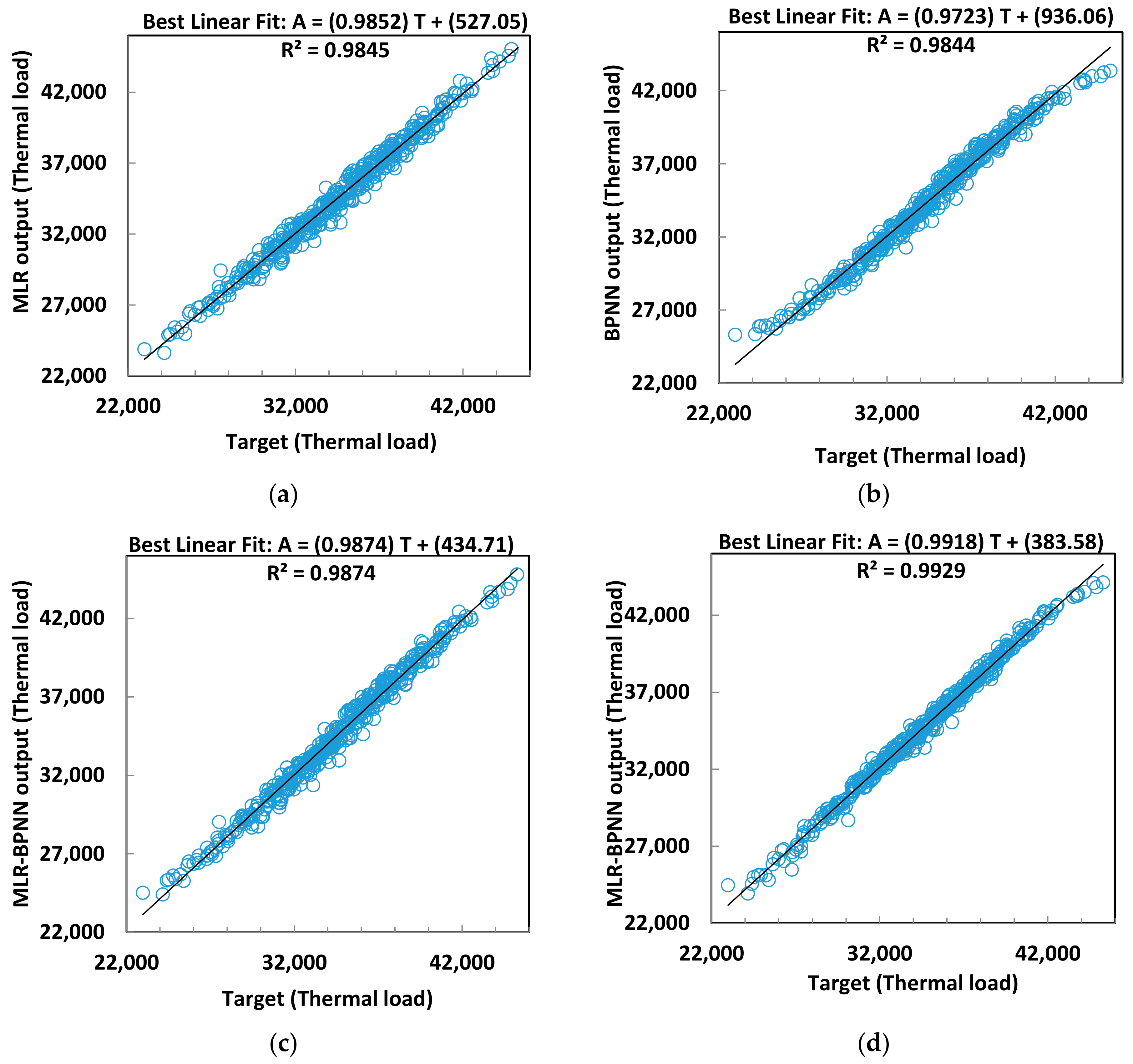
Figure 2.
Regression between predicted and simulated thermal load: (a) MLR model vs. (b) BPNN model vs. (c) MLR (BPNN + MLR) model vs. (d) MLR-BPNN model.
Figure 2.
Regression between predicted and simulated thermal load: (a) MLR model vs. (b) BPNN model vs. (c) MLR (BPNN + MLR) model vs. (d) MLR-BPNN model.

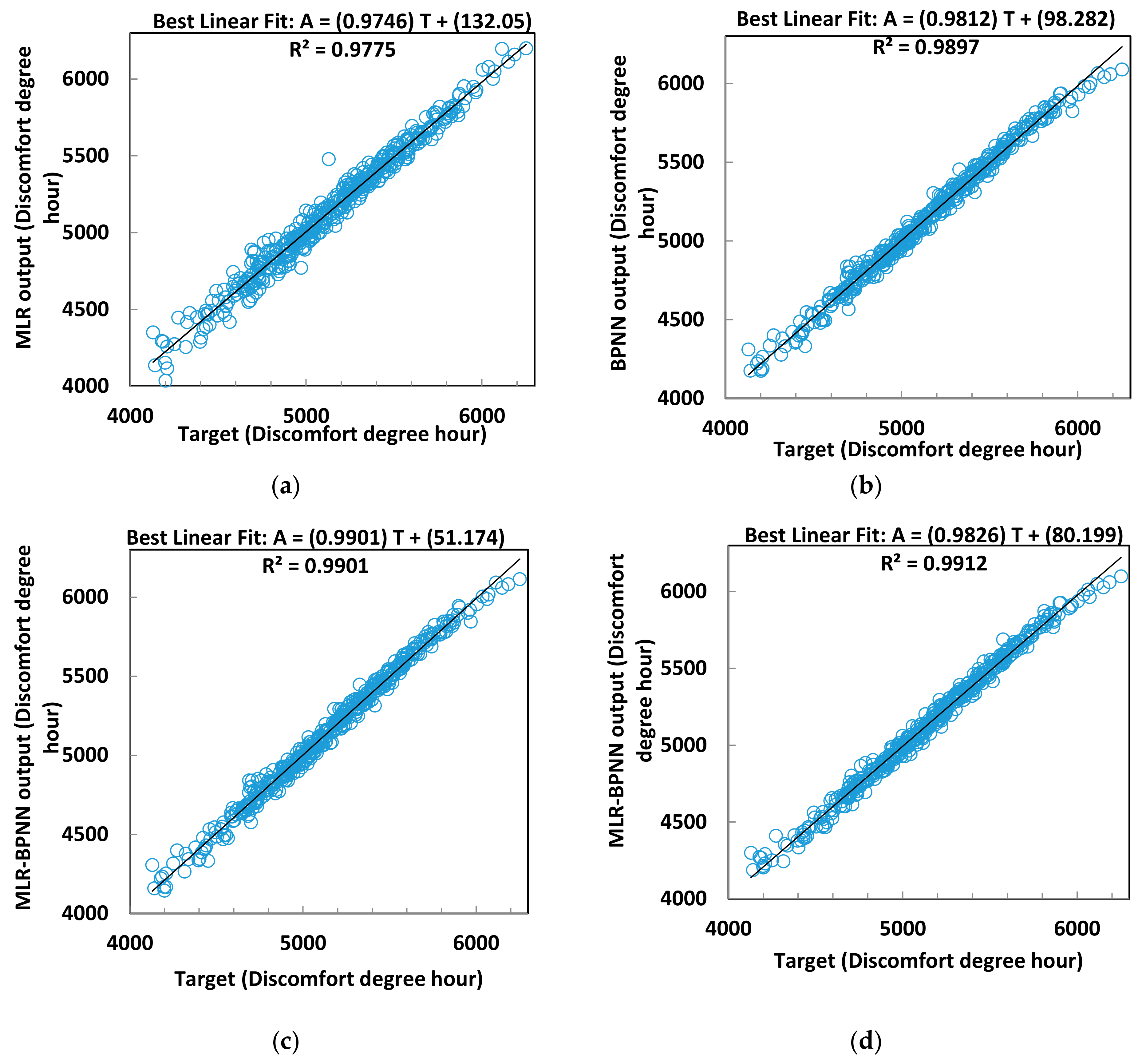
Figure 3.
Regression between predicted and simulated discomfort degree hour: (a) MLR model vs. (b) BPNN model vs. (c) MLR (BPNN + MLR) model vs. (d) MLR-BPNN model.
Figure 3.
Regression between predicted and simulated discomfort degree hour: (a) MLR model vs. (b) BPNN model vs. (c) MLR (BPNN + MLR) model vs. (d) MLR-BPNN model.


Table 1.
Groups and ranges of the independent variables.
| Group | Variable | Range |
|---|---|---|
| Window-to-wall ratio (WWR) (%) | East (x1) | [10, 80] |
| South (x2) | [10, 80] | |
| West (x3) | [10, 80] | |
| North (x4) | [10, 80] | |
| Absorptance of solar radiation (-) | East (x5) | [0.1, 0.9] |
| South (x6) | [0.1, 0.9] | |
| West (x7) | [0.1, 0.9] | |
| North (x8) | [0.1, 0.9] | |
| Roof (x9) | [0.1, 0.9] | |
| Insulation thickness (mm) | East (x10) | [10, 100] |
| South (x11) | [10, 100] | |
| West (x12) | [10, 100] | |
| North (x13) | [10, 100] | |
| Roof (x14) | [10, 100] | |
| Concrete thickness (m) | East (x15) | [0.05, 0.25] |
| South (x16) | [0.05, 0.25] | |
| West (x17) | [0.05, 0.25] | |
| North (x18) | [0.05, 0.25] | |
| Roof (x19) | [0.05, 0.25] |
Table 2.
Comparisons of different thermal load models.
| Method | Annual Thermal Load | |||||
|---|---|---|---|---|---|---|
| MAE | Std_AE | MAPE | Std_APE | Correlation Coefficient | ||
| MLR | Training | 407.466 | 323.542 | 1.20% | 0.98% | 0.992 |
| Validation | 353.344 | 301.33 | 1.05% | 0.92% | 0.996 | |
| CHAID | Training | 1250.547 | 1031.06 | 3.73% | 3.28% | 0.921 |
| Validation | 1172.815 | 936.546 | 3.30% | 2.53% | 0.925 | |
| ECHAID | Training | 1349.885 | 1055.335 | 3.98% | 3.23% | 0.905 |
| Validation | 1352.991 | 1161.781 | 4.07% | 3.73% | 0.938 | |
| BPNN | Training | 391.802 | 347.656 | 1.16% | 1.10% | 0.992 |
| Validation | 345.591 | 315.275 | 0.93% | 0.79% | 0.995 | |
| RBFN | Training | 751.735 | 600.471 | 2.24% | 1.92% | 0.972 |
| Validation | 777.938 | 493.956 | 2.25% | 1.85% | 0.979 | |
| CART | Training | 1218.253 | 901.409 | 3.59% | 2.72% | 0.93 |
| Validation | 1229.29 | 921.737 | 3.55% | 2.70% | 0.932 | |
| SVM | Training | 3265.099 | 2424.049 | 9.78% | 8.13% | 0.962 |
| Validation | 3548.173 | 2381.617 | 10.27% | 7.04% | 0.971 | |
Table 3.
Comparisons of different discomfort degree hour models.
| Method | Discomfort Degree Hour | |||||
|---|---|---|---|---|---|---|
| MAE | Std_AE | MAPE | Std_APE | Correlation Coefficient | ||
| MLR | Training | 47.37 | 39.893 | 0.94% | 0.84% | 0.988 |
| Validation | 48.705 | 36.495 | 0.97% | 0.78% | 0.993 | |
| CHAID | Training | 117.837 | 96.879 | 2.32% | 1.94% | 0.93 |
| Validation | 126.764 | 93.498 | 2.41% | 1.73% | 0.912 | |
| ECHAID | Training | 123.334 | 103.691 | 2.40% | 2.03% | 0.916 |
| Validation | 139.876 | 84.034 | 2.75% | 1.72% | 0.948 | |
| BPNN | Training | 31.733 | 28.563 | 0.63% | 0.58% | 0.995 |
| Validation | 26.597 | 19.995 | 0.50% | 0.37% | 0.997 | |
| RBFN | Training | 74.806 | 60.381 | 1.48% | 1.22% | 0.972 |
| Validation | 82.075 | 64.422 | 1.57% | 1.22% | 0.976 | |
| CART | Training | 117.713 | 90.906 | 2.30% | 1.80% | 0.932 |
| Validation | 166.616 | 101.718 | 2.57% | 1.97% | 0.926 | |
| SVM | Training | 294.392 | 215.663 | 5.80% | 4.42% | 0.970 |
| Validation | 336.008 | 209.413 | 6.45% | 3.91% | 0.975 | |
Table 4.
Percentage of cases when error falls into the given range for thermal load model.
| Relative Error | Method | <1% | <2.5% | <5% | <10% | <25% | Average (%) |
|---|---|---|---|---|---|---|---|
| Percentage of cases when error falls into the range | MLR | 51.1% | 89.6% | 99.6% | 100.0% | 100.0% | 1.19 |
| CHAID | 20.2% | 41.1% | 76.0% | 95.3% | 100.0% | 3.68 | |
| ECHAID | 17.1% | 40.2% | 70.9% | 94.4% | 100.0% | 3.99 | |
| BPNN | 54.7% | 90.7% | 99.1% | 99.8% | 100.0% | 1.14 | |
| RBFN | 30.9% | 64.7% | 91.3% | 99.6% | 100.0% | 2.24 | |
| CART | 19.3% | 40.4% | 72.2% | 96.9% | 100.0% | 3.58 | |
| SVM | 6.9% | 16.7% | 32.7% | 59.1% | 94.2% | 9.83 |
Table 5.
Percentage of cases when error falls into the given range for discomfort degree hour model.
Table 5.
Percentage of cases when error falls into the given range for discomfort degree hour model.
| Relative Error | Method | <1% | <2.5% | <5% | <10% | <25% | Average (%) |
|---|---|---|---|---|---|---|---|
| Percentage of cases when error falls into the range | MLR | 63.8% | 95.6% | 99.6% | 100.0% | 100.0% | 0.94 |
| CHAID | 28.2% | 63.1% | 89.1% | 99.6% | 100.0% | 2.33 | |
| ECHAID | 28.9% | 59.6% | 87.3% | 100.0% | 100.0% | 2.44 | |
| BPNN | 82.4% | 98.2% | 100.0% | 100.0% | 100.0% | 0.62 | |
| RBFN | 42.2% | 82.4% | 98.2% | 100.0% | 100.0% | 1.48 | |
| CART | 29.3% | 62.0% | 89.3% | 100.0% | 100.0% | 2.32 | |
| SVM | 9.6% | 25.8% | 51.3% | 84.4% | 100.0% | 5.86 |
Table 6.
Performance evaluation for the MLR-BPNN method.
| Item | MAE | Std_AE | MAPE | Std_APE | Correlation Coefficient | |
|---|---|---|---|---|---|---|
| Annual thermal load | Training | 276.351 | 233.472 | 0.82% | 0.74% | 0.996 |
| Validation | 269.644 | 266.650 | 0.76% | 0.73% | 0.996 | |
| Discomfort degree hour | Training | 30.355 | 26.563 | 0.60% | 0.54% | 0.995 |
| Validation | 29.233 | 20.537 | 0.55% | 0.39% | 0.998 | |
Table 7.
Percentage of cases where the error falls into the given range.
| Relative Error | Method | Item | <1% | <2.5% | <5% | <10% | <25% | Average (%) |
|---|---|---|---|---|---|---|---|---|
| Percentage of cases when error falls into the range | MLR (MLR + BPNN) | Annual thermal load | 56.9% | 93.3% | 99.1% | 100.0% | 100.0% | 1.05 |
| Discomfort degree hour | 82.2% | 98.7% | 100.0% | 100.0% | 100.0% | 0.61 | ||
| MLR-BPNN | Annual thermal load | 69.8% | 97.8% | 99.8% | 100.0% | 100.0% | 0.82 | |
| Discomfort degree hour | 82.7% | 99.6% | 100.0% | 100.0% | 100.0% | 0.59 |
© 2018 by the authors. Licensee MDPI, Basel, Switzerland. This article is an open access article distributed under the terms and conditions of the Creative Commons Attribution (CC BY) license (http://creativecommons.org/licenses/by/4.0/).
Share and Cite
MDPI and ACS Style
Lin, Y.; Zhou, S.; Yang, W.; Shi, L.; Li, C.-Q. Development of Building Thermal Load and Discomfort Degree Hour Prediction Models Using Data Mining Approaches. Energies 2018, 11, 1570. https://doi.org/10.3390/en11061570
AMA Style
Lin Y, Zhou S, Yang W, Shi L, Li C-Q. Development of Building Thermal Load and Discomfort Degree Hour Prediction Models Using Data Mining Approaches. Energies. 2018; 11(6):1570. https://doi.org/10.3390/en11061570
Chicago/Turabian StyleLin, Yaolin, Shiquan Zhou, Wei Yang, Long Shi, and Chun-Qing Li. 2018. "Development of Building Thermal Load and Discomfort Degree Hour Prediction Models Using Data Mining Approaches" Energies 11, no. 6: 1570. https://doi.org/10.3390/en11061570
Note that from the first issue of 2016, this journal uses article numbers instead of page numbers. See further details here.