Coordination and Control of Building HVAC Systems to Provide Frequency Regulation to the Electric Grid

1
Computational Sciences and Engineering Division, Oak Ridge National Laboratory, Oak Ridge, TN 37831, USA
2
Energy and Transportation Science Division, Oak Ridge National Laboratory, Oak Ridge, TN 37831, USA
*
Author to whom correspondence should be addressed.
†
These authors contributed equally to this work.
Energies 2018, 11(7), 1852; https://doi.org/10.3390/en11071852
Submission received: 11 June 2018
/
Revised: 6 July 2018
/
Accepted: 9 July 2018
/
Published: 16 July 2018
(This article belongs to the Special Issue Intelligent Control in Energy Systems)
Abstract
:Buildings consume 73% of electricity produced in the United States and, currently, they are largely passive participants in the electric grid. However, the flexibility in building loads can be exploited to provide ancillary services to enhance the grid reliability. In this paper, we investigate two control strategies that allow Heating, Ventilation and Air-Conditioning (HVAC) systems in commercial and residential buildings to provide frequency regulation services to the grid while maintaining occupants comfort. The first optimal control strategy is based on model predictive control acting on a variable air volume HVAC system (continuously variable HVAC load), which is available in large commercial buildings. The second strategy is rule-based control acting on an aggregate of on/off HVAC systems, which are available in residential buildings in addition to many small to medium size commercial buildings. Hardware constraints that include limiting the switching between the different states for on/off HVAC units to maintain their lifetimes are considered. Simulations illustrate that the proposed control strategies provide frequency regulation to the grid, without affecting the indoor climate significantly.
1. Introduction
To ensure the functionality and reliability of a power grid, supply and demand must be balanced instantaneously and continuously. Balancing generation and load at all time scales, given the randomness in dynamics of generation and demand, is challenging. Correcting the mismatch requires ancillary services such as regulation and load following. The Federal Energy Regulatory Commission (FERC) has defined such services as those “necessary to support the transmission of electric power from seller to purchaser given the obligations of control areas and transmitting utilities within those control areas to maintain reliable operation of the interconnected transmission system.” This quotation highlights the importance of ancillary services for both bulk-power reliability and support of commercial transactions [1]. Furthermore, a large amount of ancillary service will be required in the future if a large fraction of the energy needs is to be met from renewable energy sources with their associated unpredictability and volatility.
The traditional electric grid is load-following and is based on centralized generation assets that are controlled to compensate for demand changes in order to maintain a stable and reliable grid. Higher penetration of renewables and distributed energy resources, with their uncontrollable generation variability, imposes significant grid stability and control challenges. Demand-side control techniques are expected to address these challenges by increasing reliability and stability, reducing reserve margins, reducing peak demand, and improving energy efficiency. The inherent flexibility of many electric loads, when harnessed without impacting consumer comfort, can be an inexpensive source of ancillary service. Although employing loads for system services raise several challenges, several key advantages can be achieved: (i) reducing overall grid emissions by using loads to provide system services [2]; (ii) instantaneous response of loads to operator requests, versus slow response of generators to make significant output changes [3]; and (iii) less variability associated to a very large number of small loads with respect to that of a small number of large generators [3]. The key technical impediments to reliable utilization of loads for system services are the development of deployable control strategies over wide-area and the development of inexpensive and scalable sensing, communication, and control infrastructure [4].
Buildings account for 73% of total electricity consumption in the United States and therefore will play a crucial role in the future of the national electric power system. Total annual US energy consumptions are roughly equal for residential and commercial buildings with Heating, Ventilation and Air-Conditioning (HVAC) loads that account for about half of their energy use. Nonetheless, only about 10% of all commercial buildings use automation systems to control their energy usage, and an insignificant percentage of these buildings provide ancillary services to power system operators [5]. The unrealized potential to incorporate buildings into the grid to provide ancillary services is therefore very large and will help mitigate the global challenge of providing reliable, cost effective, and clean energy.
The use of commercial building HVAC systems for providing ancillary services ia examined in [6,7,8,9,10,11,12,13,14,15,16,17,18]. In particular, the works in [6,7,8] address the usage of commercial buildings for demand response programs, which typically involve reduction of peak power in emergency situations. The works in [9,10,11,12] illustrate the potential promise of model predictive control (MPC) for energy efficiency in buildings and for integrating time-of-use rates for shifting loads. The work in [13] shows that the supply fans in air handling units (AHUs) with variable frequency drives (VFDs) can provide high frequency ancillary service of about 70% of the regulation reserves in the time scale of 8 s to 3 min. In [14], the time scale of ancillary service from commercial building HVAC systems is extended to the range of 3 min to 1 h by using the flexibility in the power demand from chillers. Recent research on residential loads [19,20] such as HVAC and refrigerators has shown that such loads can provide ancillary service with the help of appropriate control algorithms. One drawback of residential loads is that they are largely on/off control, which greatly reduces the flexibility of control strategies that can be applied. Such a drawback will be tackled for the first time in this paper by considering a coordination and control of an aggregate of on/off loads to provide desired grid-response. In particular, the proposed controller will manipulate the total power consumption of available HVAC loads according to requested change in power from the grid side, represented by a regulation signal, to enhance the grid reliability and stability.
In this paper, we consider HVAC loads as an ancillary service for providing frequency regulation to the grid. We investigate two control strategies of HVAC systems to provide such services. In the first strategy, we consider an optimal strategy based on MPC acting on a continuously variable HVAC system, which is available in most large commercial buildings. MPC has been widely employed in energy efficiency in buildings, but only a few in control strategies for ancillary services to the grid. In the second strategy, we consider rule-based coordination and control of an aggregate of on/off HVAC systems, which are widely-spread in residential buildings in addition to many small to medium commercial buildings. This strategy is based on priority control of room temperatures of multiple on/off HVAC systems. Numerical results show that it is feasible to use a small portion (less than 20%) of the total HVAC power in residential/commercial buildings for regulation services to the grid, with little change in their indoor environments.
2. HVAC Thermal Dynamical Model
In this section, a simple, yet realistic building thermal model is introduced to represent the building with a HVAC system. It is a continuous-time linear time-invariant (LTI) system model based on the dynamics of the room temperature, interior-wall surface temperature, and exterior-wall core temperature. This physics-based lumped thermal model is initially proposed in [21] and employed in [22,23,24] for simulating residential and commercial buildings. It is described by
where the variables used in the above model are defined in Table 1, and the parameter values are provided in Table 2.
The system states are , , and . The model inputs are divided into manipulated variables and disturbance inputs. The manipulated variables are the cooling power and the heating power , and they can be combined to one variable . Without loss of generality, we assume cooling and heating are not functioning simultaneously in our study, which is usually the case for small residential buildings. The disturbances are and .
Define the state vector x, the control signal vector u, and the environment stochastic disturbance vector as:
The continuous-time state-space model can then be described compactly as:
where
We consider the discrete-time (sampled) version of Equation (1) described by
where k is the discrete-time index, and the parameters are computed from the continuous-time model parameters in (2).
The control input u is the critical actuator yielding its own working properties and conditions. It takes continuous values within a certain bound for a given HVAC system in large commercial buildings, where the variable frequency drive (VFD), which is available in variable air volume (VAV) HVAC systems and allows continuous input power, is responsible for changing the air handling unit fan speed. On the other hand, the control input u takes discrete values, usually two to three states, in the on/off HVAC systems that are available in residential buildings in addition to many small to medium commercial buildings. In this paper, both the VAV and on/off HVAC systems are investigated to provide ancillary services to the grid.
3. Control Design for a VAV HVAC Unit
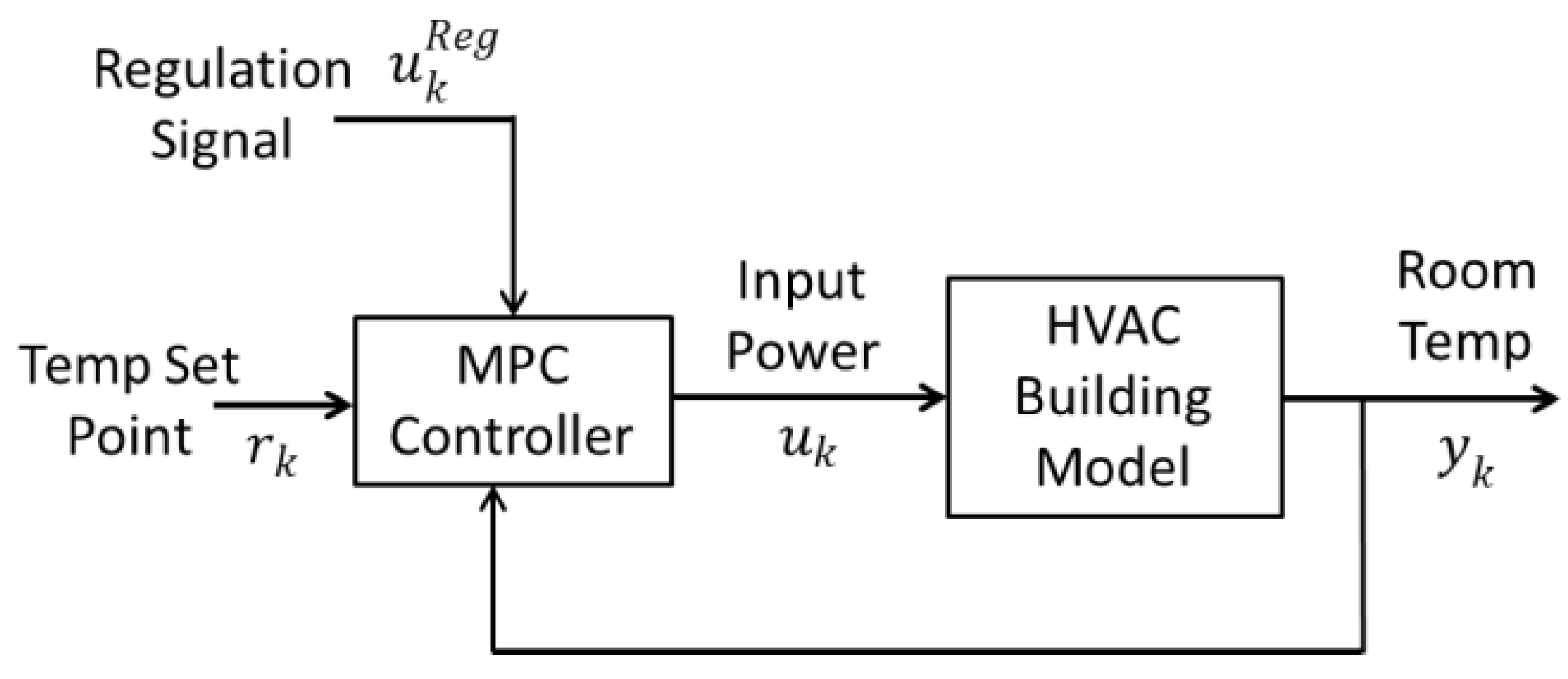
In this section, a controller is designed for a large commercial building having a VAV HVAC units with continuous control variables. The intended controller should control the operation of the HVAC unit such that: (i) the change in the power consumed by the HVAC unit is as close as reasonably possible to the requested change in power in the regulation signal for that building; and (ii) the reported thermostat temperature for the HVAC unit is as close as possible to its set point. To achieve these two objectives, we have designed the feedback control system shown in Figure 1. It is an MPC strategy that is widely-used in the industry and displays its main strength when applied to problems with constraints imposed on both the manipulated and controlled variables. The designed controller has three input signals and one output signal. The input signals are the room temperature set point , the regulation signal , and the current reported room (thermostat) temperature ( represents of the thermal model in Equation (3), the other model states are assumed to be non-measurable). The output signal of the controller is a scaled version of the input power to the HVAC unit, . The plant represents the discrete-time thermal model for the HVAC and building system described in Equation (3).
The controller minimizes the cost function described by
subject to
where k is the current control interval, p is the prediction horizon, is the predicted value of room temperature at ith prediction horizon step, is the thermostat set point at ith prediction horizon step, is the tuning weight for the room temperature at ith prediction horizon step, is the estimated value (to be computed) of the input power to the HVAC unit (manipulated variable) at ith prediction horizon step, is the target value for the manipulated variable at ith prediction horizon step, is the tuning weight for the manipulated variable at ith prediction horizon step, and .
The values , and are controller specifications, and are constants. The controller receives and values for the entire horizon and uses the state observer to predict the plant outputs. At instant k, the controller state estimates are available, thus J is a function of only. Since the regulation signal represents the change in the power consumed by the HVAC unit, is described by
where is the optimal value for the manipulated variable at ith prediction horizon step without considering the impact of the regulation signal, i.e. the optimal control signal such that the room air temperature is as close as possible to its set point.
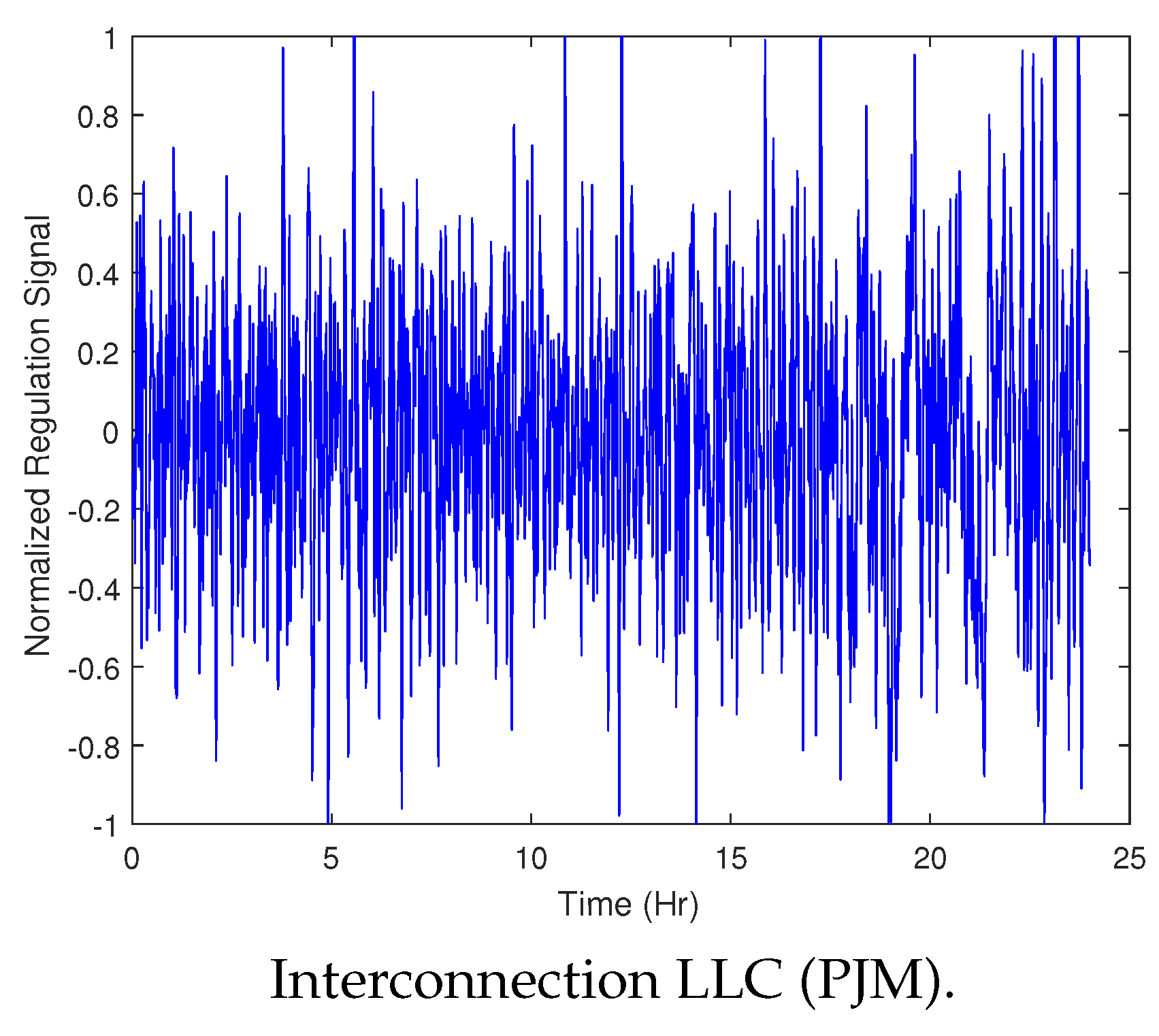
The regulation signal used in our analysis is taken from the PJM dynamic (D) regulation control signal, which is used for fast-responding resources and constructed from the area control error (ACE) that measures the amount of negative or positive power needed in the power system [25]. Figure 2 shows the normalized regulation signal for a specific day that is sampled every 1 min. A positive ACE value represents the case where an increase in the power consumption is requested and a negative value represents the case where a decrease in the power consumption is requested. The regulation signal can simply be distributed among multiple VAV HVAC units by maintaining its shape and scaling it down to proper levels to maintain occupant comfort. Thanks to the continuous input power ability of VAV HVAC systems that allows this simple distribution of the regulation signal among multiple HVAC units. Thus, without loss of generality, we only consider one VAV HVAC unit in the analysis presented next.
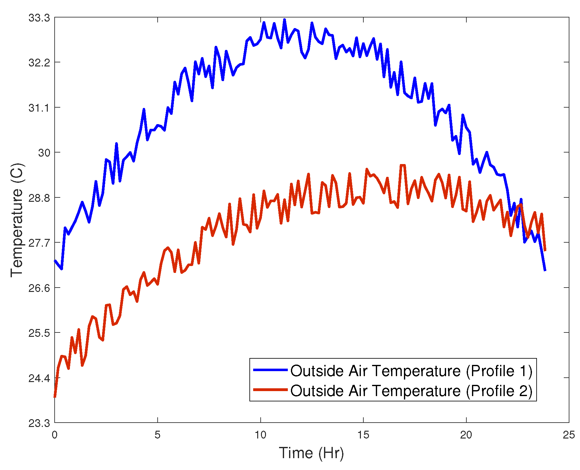
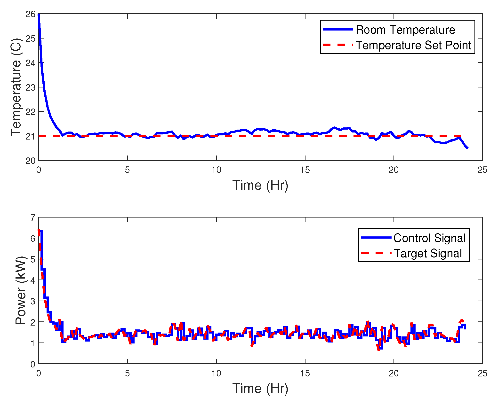
To illustrate the performance of the control scheme in Equations (4)–(6), simulations are conducted for a typical summer day with the following setup: simulation time-step is selected to be one minute to satisfy the variations in the regulation signal, initial room temperature C, room temperature set point C, C C, kW (cooling scenario), , and the outside air temperature (profile 1) demonstrated in Figure 3 is considered. The random noise that exists in the temperature profile represents changes in solar irradiance due to temporary cloud cover.
The simulation results for this scenario are demonstrated in Figure 4, where the lower graph shows that the change in the power consumed by the HVAC unit closely follows the regulation signal, while the room temperature is close enough to the temperature set point (within C) , as shown in the upper graph. Note that, in this example, the maximum power in the regulation signal is 1 kW, which is about 17% of the maximum power consumed by an HVAC unit (6 kW).
Table 3 illustrates the performance of the designed MPC controller for this scenario over different regulation power levels. We observe that the requested change in power (maximum regulation signal magnitude) should be less than 17% of the total power consumed by the HVAC unit to maintain occupant comfort (room temperature is within C from its set point). The root-mean-square-error (RMSE) of the room temperature from its set point is also presented in Table 3.
In the next section, we introduce the second control strategy that considers coordination and control of an aggregate of on/off HVAC systems.
4. Control Design for an Aggregate of on/off HVAC Units
Now, we address the more challenging on/off HVAC system, which is widely used in residential buildings. It is obvious that an on/off HVAC system does not provide the required flexibility for tracking a regulation signal as in the VAV HVAC case because of the limited number of states in the on/off HVAC, usually two states (on and off). However, we show in this section that, by proper control and coordination of a fleet of on/off HVAC systems (available in one or many building(s)), the required flexibility for tracking a regulation signal can be reached. Thus, the objective in this case is to design a controller (strategy) for an aggregate of on/off HVAC systems that takes into consideration the regulation signal provided by the power utility such that its impact should be minimal on room temperatures of the buildings. The proposed controller should coordinate the operation of the HVAC units across all buildings such that: (i) the total change in the power consumed by all HVAC units is as close as reasonably possible to the requested change in power in the regulation signal; and (ii) the reported thermostat temperature for each HVAC unit is as close as possible to its set point. In addition, the following constraints should be satisfied:
- The on/off HVAC unit has the following three states:
- (a)
- Off (no power consumed).
- (b)
- Stage 1 cooling (power consumed is 3 kW).
- (c)
- Stage 2 cooling (power consumed is 6 kW).
- Switching between the different states for an HVAC unit is not allowed before certain time duration from the last switch (we assume it is 10 min in our analysis). This is required to maintain the lifetime of the HVAC units. More frequent switching of an HVAC unit may cause some damage to the unit and shorten its lifetime.
- Thermostat temperature control (dead band) for each building is C from its set point.
The proposed control architecture for this strategy is illustrated in Figure 5, where the feedback message from each HVAC unit to the central controller contains its current room temperature and thermostat set point, i.e. and M is the total number of HVAC units. Note that the manipulated variables, take only three values, as indicated in Constraint 1 above.
Without loss of generality, by considering the cooling case in HVAC units and assuming all buildings have the same temperature set points, the centralized rule-based control strategy is designed as follows:
- If the regulation signal is positive, this indicates an increase in the power consumption is requested (more cooling). In this case, the controller should prioritize room temperatures with the highest temperatures to cool them first. Thus, the controller should increase the power provided to HVAC units with the highest temperature zones or buildings.
- If the regulation signal is negative, this indicates a decrease in the power consumption is requested (less cooling). In this case, the controller should prioritize room temperatures with the lowest temperatures to not cool them first. Thus, the controller should decrease the power provided to HVAC units with the lowest temperature zones or buildings.
For the case where buildings have different temperature set points, the controller prioritizes room temperature deviations from their set points with the highest positive temperature deviations to cool them first when the regulation signal is positive and with the highest negative temperature deviations to not cool them first when the regulation signal is negative. It should be remarked that the home owner could very easily shift the set point if he feels cold or hot. This priority control strategy is described in Algorithm 1. Moreover, the heating case in HVAC units is designed in an opposite way, for instance, when the regulation signal is positive, the controller increases the power provided to HVAC units with the lowest temperature zones or buildings. Note that this priority control strategy is chosen based on its simplicity to implement, as it does not require solving an optimization problem such as the MPC strategy in the previous section. Thus, it is computationally efficient and much easier to implement in practice. Lastly, it is hardly fair to directly compare these two control strategies because each strategy is used for different type of HVAC loads. Using MPC for on/off HVAC loads requires solving more complicated mixed integer linear programming problem, which is out of the scope of this manuscript and is left for future work.
In the next section, numerical results are presented to illustrate the performance of the rule-based control strategy.
| Algorithm 1: The rule-based control strategy for a fleet of on/off HVAC systems (cooling case). |
 |
5. Numerical Results
We consider 50 on/off HVAC units (buildings) in our analysis with the same PJM dynamic regulation signal used in Section 3, but it is now scaled up to 50 kW to satisfy the ratio of the maximum regulation to the maximum power consumed by all HVAC units (300 kW) as described in Section 3. In addition, initial room temperatures are assumed to be normally distributed around their set points with unit variance and all HVAC units are initially at off state. In addition, the same outside temperature profile and building parameters as in Section 3 are used here. The simulation time-step is 1 min and the 10-min switching constraint of on/off HVAC units is maintained in the control strategy.
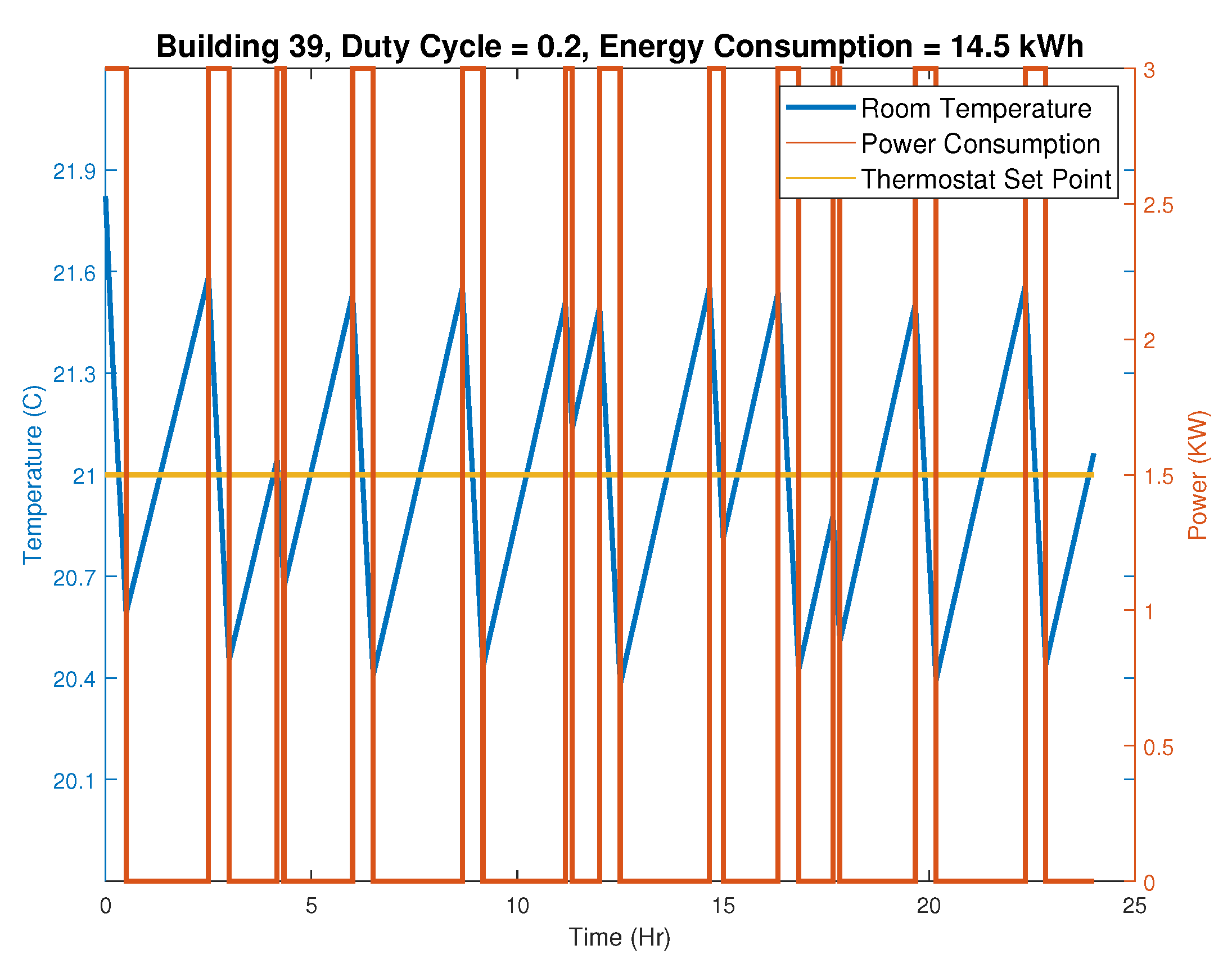
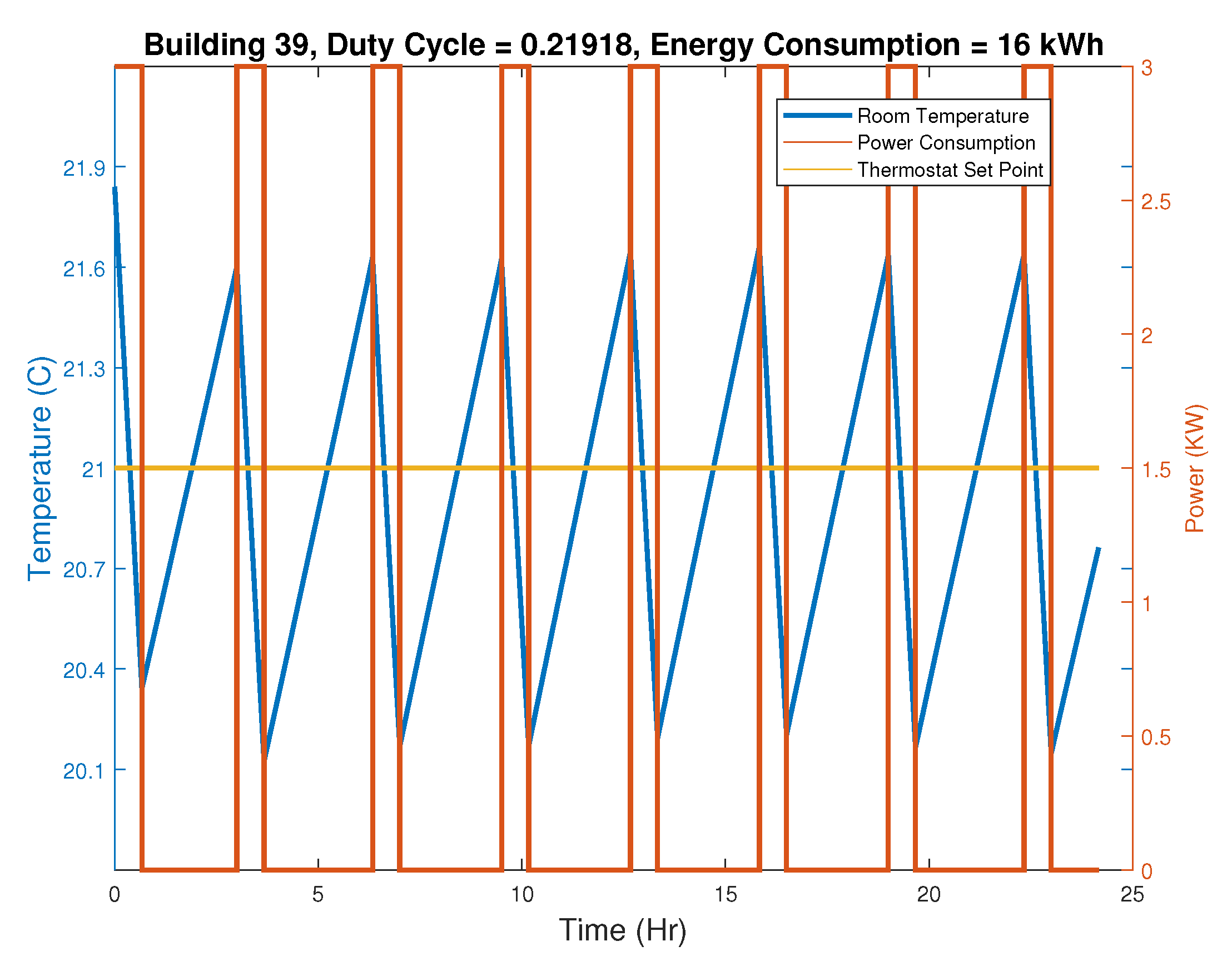
The performance of the designed rule-based control strategy has been investigated for a 24-h period and compared with the baseline case where no regulation is considered (the only objective is to satisfy the thermostat temperature for each HVAC unit). Figure 6 shows the room temperature and the corresponding power consumed by the HVAC unit for one building selected at random (Building 39). Figure 7 shows the baseline case for the same scenario in Figure 6 for comparison. Notice the variations in the room temperature under the regulation case (Figure 6) as compared with the one without regulation (Figure 7). These variations are due to the impact of satisfying the regulation condition. Despite these variations, the room temperature remained most of the time within the allowed band, which is C from the set point. In addition, it is observed that the impact of the regulation on the HVAC total power consumption and duty cycle (fraction of time in which HVAC unit is ON) is minimal (see their values on top of the figures). In addition, notice that this HVAC unit did not switch to Stage 2 cooling because of either there are higher room temperatures at that time than the one at Building 39 that have higher priorities, or the regulation signal at that time was not high enough to turn on this unit to Stage 2 cooling after taking care of the other buildings with higher room temperatures. Similar behaviors as in Building 39 are observed in the remaining buildings, except that Stage 2 cooling is observed for short time durations in few HVAC units.
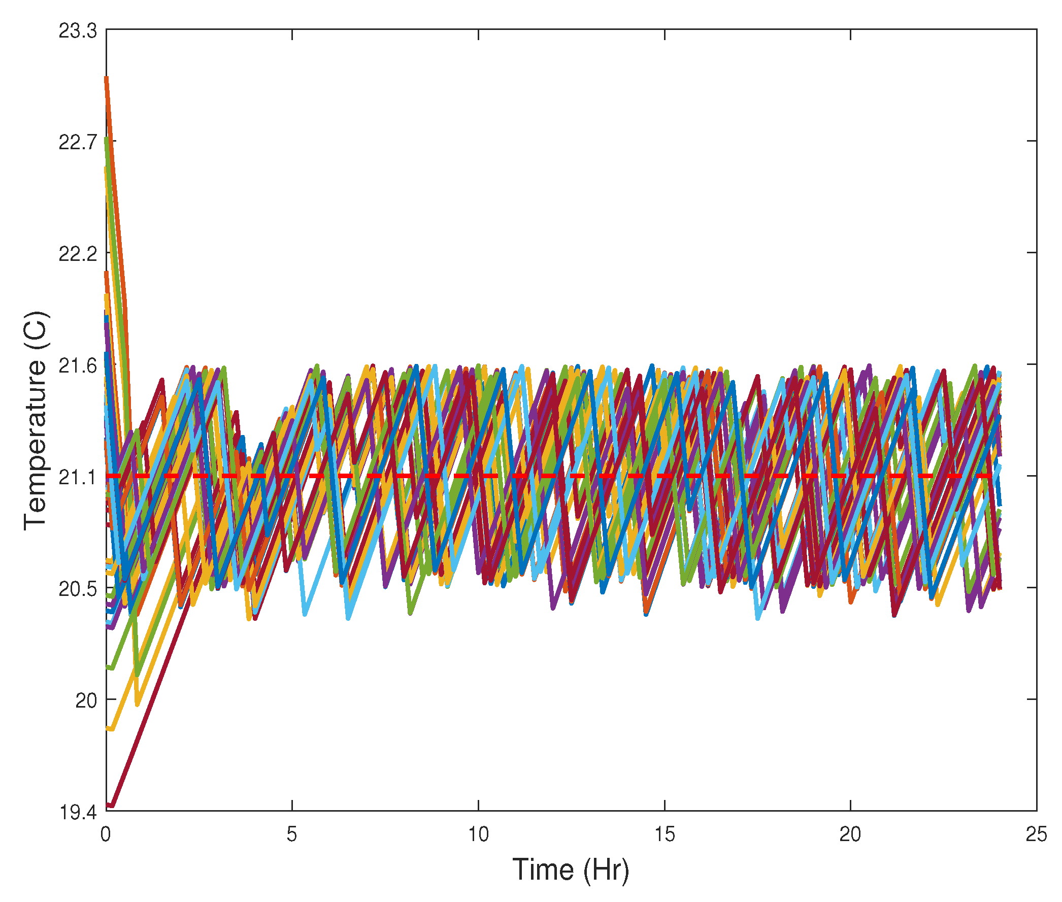
Figure 8 demonstrates room temperatures for all 50 buildings. Observe that the deviations from the set points are less than 0.5 C most of the time. This is due to the appropriate selection of the total number of buildings (and their corresponding maximum power consumption) relative to the maximum regulation power.
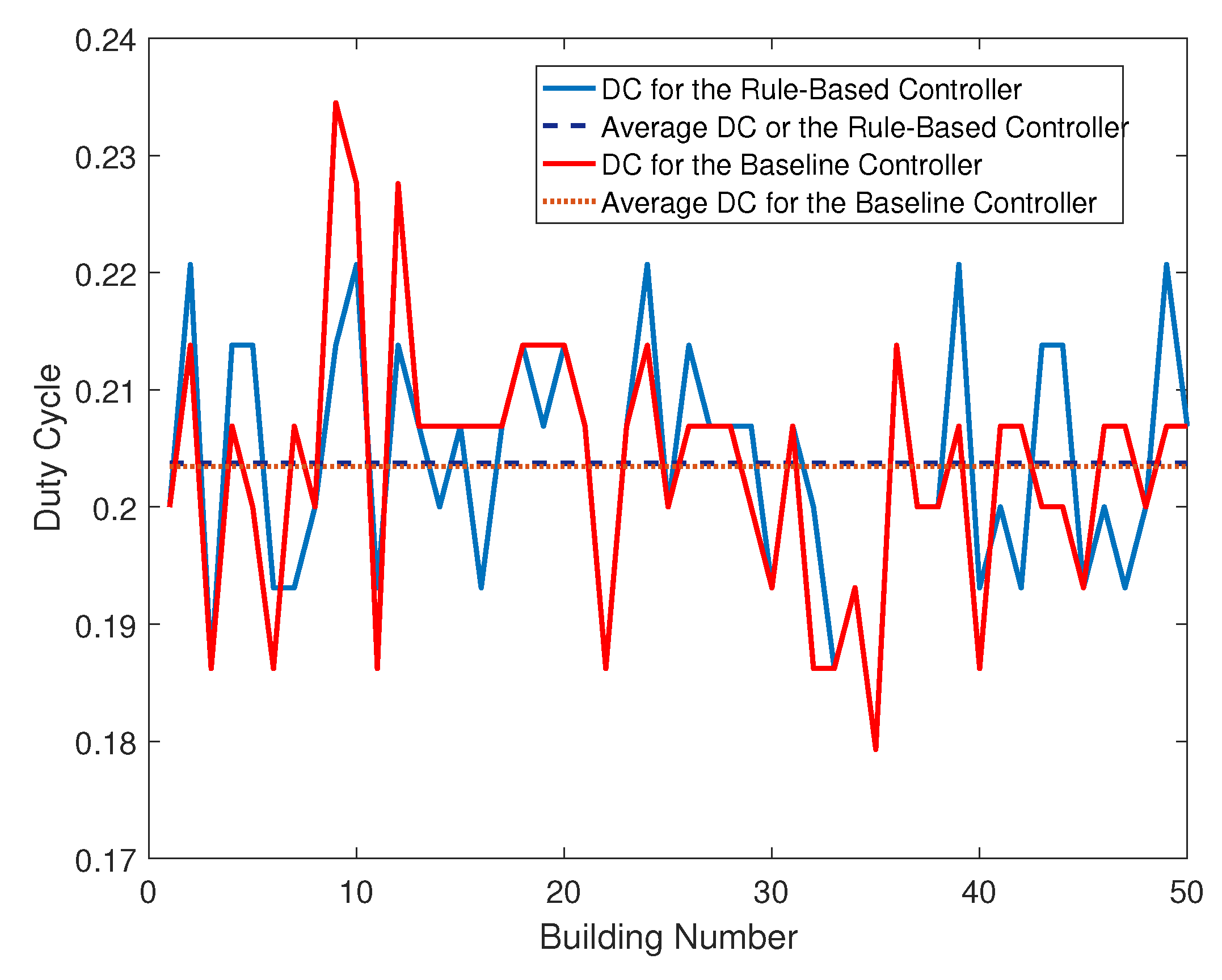
Figure 9 shows the HVAC duty cycles (DCs) for the 50 buildings using the rule-based and baseline controllers. Notice that about 20% duty cycle is typical for a hot summer day. It can be observed that nearly all buildings provide the same amount of ancillary service. The average duty cycles for all buildings for the designed rule-based and baseline controllers are 0.2037 and 0.2034, respectively. These duty cycles correspond to total energy consumption by all 50 buildings for 24-h interval of an amount 741.5 kWh and 737 kWh, respectively. Notice that nearly the same duty cycle (power consumption) took place for both scenarios. Assuming the utility pays 10 cents per kWh for building owners subscribed to provide ancillary service to the grid, the owners of the 50 buildings in this scenario will receive credit of $798 per month.
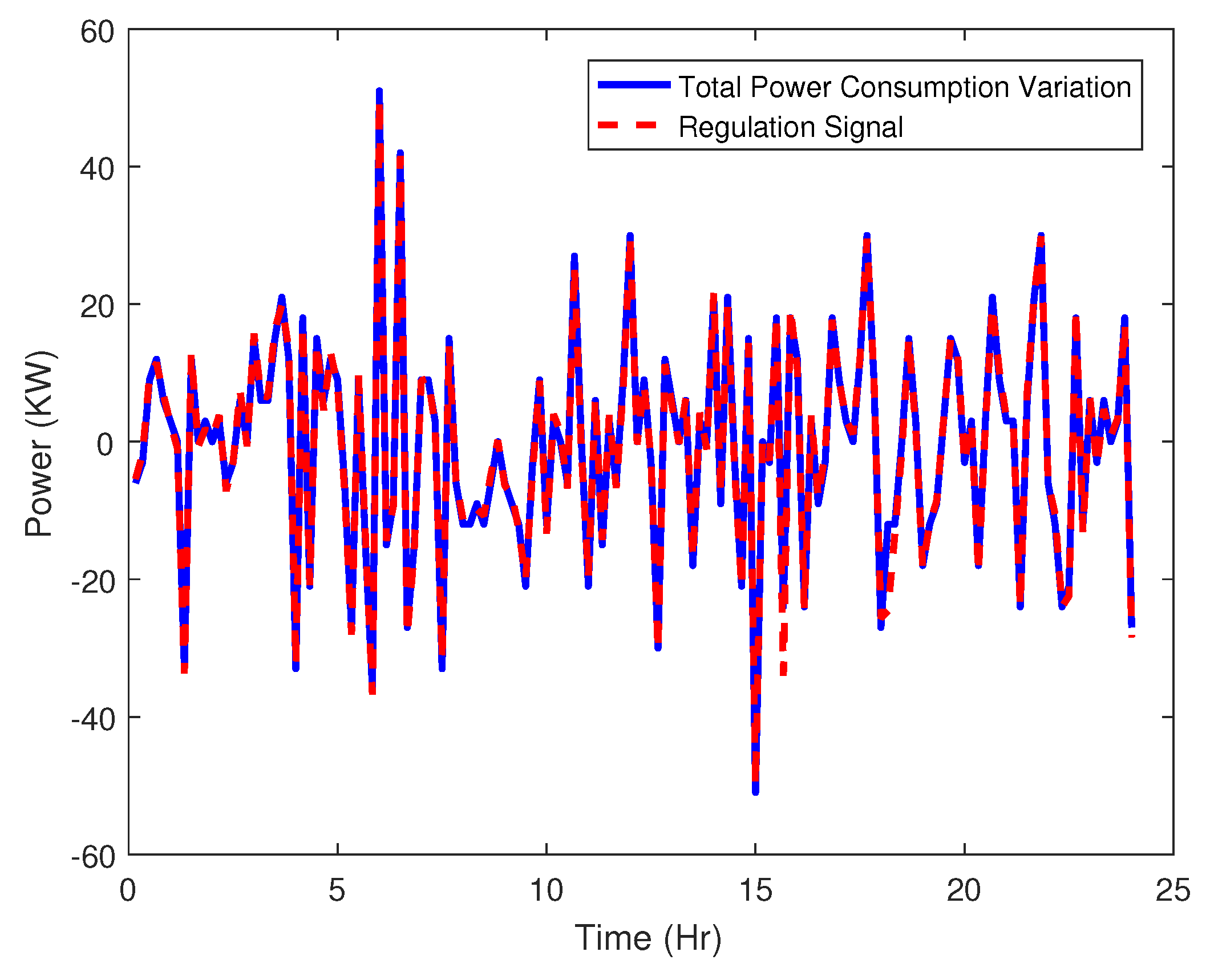
Figure 10 demonstrates that the total power consumed by all 50 buildings closely follows the regulation signal. This is due to the proper designed control strategy and the appropriate selection of the total number of buildings relative to the maximum regulation power.
Sensitivity analysis has been conducted for the designed rule-based controller under different buildings parameters ( and are within 20% tolerance from their nominal values) and outside air temperatures, where similar behaviors as in previous scenarios (Figure 6, Figure 7, Figure 8, Figure 9 and Figure 10) are observed. For example, when different building parameters and outside air temperatures are used (Profile 2 in Figure 3), numerical results show that the room temperatures for all 50 buildings are within C from their set points almost all of the time while satisfying the required regulation, as illustrated in Figure 11.
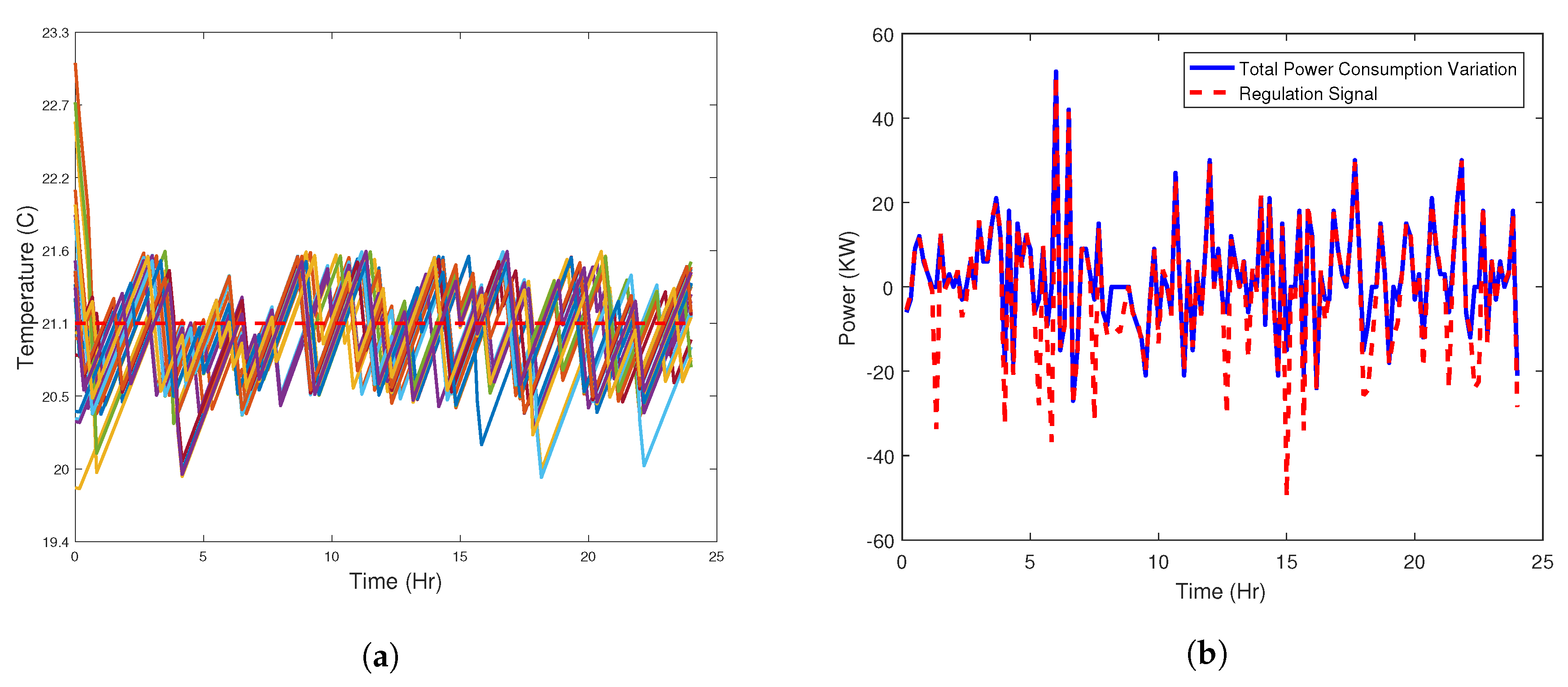
It is also interesting to investigate the impact of the total number of buildings on the performance of the rule-based control strategy. Figure 12 illustrates the room temperatures and aggregate power consumption variations when the total number of buildings is reduced to the half (25 buildings). We can observe that the performance in this scenario is not as good as the 50 buildings scenario; quite few room temperatures went out of the C band for some time and the aggregate power consumption variation for all building did not fully follow the regulation signal. This unsatisfactory performance is due to the fact that each HVAC unit contributed about 33% of its power capacity as an ancillary service to the grid, where our analysis for this particular example (in Section 3 and in this section as well) indicates that each HVAC unit should not contribute more than 17% of its power capacity as ancillary service to the grid to ensure satisfactory performance. It should be mentioned that we assume all the buildings have correct sizing of the HVAC system. In practice, it is also worth investigating the system sizing problem [26,27] before looking into the proposed control strategy.
Table 4 shows the maximum deviation and root-mean-square-error (RMSE) of the regulation signal and indoor temperature tracking for all buildings. Notice the improved performance with the increased number of recruited buildings, which provides additional flexibility for tracking the regulation signal and thus satisfying the grid requirements. Note that the 17% contribution limit of HVAC power capacity as ancillary service to the grid is specific to this particular example (specific to the assigned building parameters and disturbances) and should be verified/tested for different settings. Therefore, an initial testing/tuning is recommended before implementing the proposed rule-based controller to ensure satisfactory performance.
6. Conclusions and Future Directions
We have investigated two control strategies for HVAC units to provide ancillary services to the grid. In the first strategy, an optimal control based on MPC acting on a VAV HVAC unit is examined, while, in the second strategy, a rule-based control of a fleet of on/off HVAC units is examined. The presented analysis has validated our argument that coordination and control of a fleet of on/off HVAC units provide the required flexibility for ancillary services to the grid, with little impact on indoor environments. If we assume the regulation requirement of the United States is 1% of its peak load (similar to the one in PJM), the total regulation reserves that are potentially available from all residential/commercial buildings in the US are about three times of the total regulation capacity currently needed [28].
The novelty of the analysis is to use HVAC loads as ancillary service to the grid. In particular, the proposed controller should manipulate the total power consumption of available HVAC loads according to requested change in power from the grid side, represented by a regulation signal, to enhance the grid reliability and stability. The designed rule-based controller can be implemented in a centralized mode, where each building communicates its current state (room temperature, power consumption, and temperature set point) to a centralized aggregator that selects the next states of the HVAC units. Then, the selected strategies are communicated back to buildings (smart thermostats) to be applied. For large number of buildings, a cluster tree topology would be more feasible, as each building communicates its current state to a server node within its cluster, and the server nodes communicate their aggregate information to a centralized node where the control strategies are chosen and communicated back to the buildings through the cluster nodes. Another implementation option could be through the cloud, where the information is shared (via the Internet) and analyzed in utility or third-party data centers.
Future work is to conduct further studies to design a decentralized framework for the rule-based control strategy.
Author Contributions
Conceptualization, M.O., T.K. and J.N.; Methodology, M.O., T.K. and J.N.; Software, M.O. and J.D.; Validation, M.O. and J.D.; Formal Analysis, M.O. and T.K.; Investigation, M.O. and T.K.; Writing—Original Draft Preparation, M.O.; Writing—Review & Editing, J.N. and J.D.
Acknowledgments
This manuscript has been authored by UT-Battelle, LLC under Contract No. DE-AC05-00OR22725 with the U.S. Department of Energy. This material is based upon work supported by the U.S. Department of Energy, Office of Energy Efficiency and Renewable Energy. The United States Government retains and the publisher, by accepting the article for publication, acknowledges that the United States Government retains a non-exclusive, paid-up, irrevocable, world-wide license to publish or reproduce the published form of this manuscript, or allow others to do so, for United States Government purposes. The Department of Energy will provide public access to these results of federally sponsored research in accordance with the DOE Public Access Plan (http://energy.gov/downloads/doe-public-access-plan).
Conflicts of Interest
The authors declare no conflict of interest.
References
- Kirby, B.J. Frequency Regulation Basics and Trends; United States Department of Energy: Washington, DC, USA, 2005.
- Strbac, G. Demand side management: Benefits and challenges. Energy Policy 2008, 36, 4419–4426. [Google Scholar] [CrossRef]
- Kirby, B.J. Spinning Reserve from Responsive Loads; United States Department of Energy: Washington, DC, USA, 2003.
- Woo, C.K.; Kollman, E.; Orans, R.; Price, S.; Horii, B. Now that California has AMI, what can the state do with it? Energy Policy 2008, 36, 1366–1374. [Google Scholar] [CrossRef]
- Kelso, J.D. Buildings Energy Data Book; United States Department of Energy: Washington, DC, USA, 2017.
- Pavlak, G.S.; Henze, G.P.; Cushing, V.J. Optimizing commercial building participation in energy and ancillary service markets. Energy Build. 2014, 81, 115–126. [Google Scholar] [CrossRef]
- Zhao, P.; Henze, G.P.; Plamp, S.; Cushing, V.J. Evaluation of commercial building HVAC systems as frequency regulation providers. Energy Build. 2013, 67, 225–235. [Google Scholar] [CrossRef]
- Kiliccote, S.; Piette, M.A.; Hansen, D. Advanced Controls and Communications for Demand Response and Energy Efficiency in Commercial Buildings; Lawrence Berkeley National Laboratory: Berkeley, CA, USA, 2006. [Google Scholar]
- Maasoumy, M.; Sanandaji, B.M.; Sangiovanni-Vincentelli, A.; Poolla, K. Model predictive control of regulation services from commercial buildings to the smart grid. In Proceedings of the 2014 American Control Conference, Portland, OR, USA, 4–6 June 2014; pp. 2226–2233. [Google Scholar]
- Maasoumy, M.; Sangiovanni-Vincentelli, A. Total and peak energy consumption minimization of building hvac systems using model predictive control. IEEE Des. Test Comput. 2012, 29, 26–35. [Google Scholar] [CrossRef]
- Oldewurtel, F.; Ulbig, A.; Parisio, A.; Andersson, G.; Morari, M. Reducing peak electricity demand in building climate control using real-time pricing and model predictive control. In Proceedings of the 49th IEEE Conference on Decision and Control, Atlanta, GA, USA, 15–17 December 2010; pp. 1927–1932. [Google Scholar]
- Maasoumy, M.; Sangiovanni-Vincentelli, A. Optimal control of building hvac systems in the presence of imperfect predictions. In Proceedings of the Dynamics and Systems and Control Conference, Fort Lauderdale, FL, USA, 17–19 October 2012; pp. 257–266. [Google Scholar]
- Hao, H.; Lin, Y.; Kowli, A.S.; Barooah, P.; Meyn, S. Ancillary service to the grid through control of fans in commercial building HVAC systems. IEEE Trans. Smart Grid 2014, 5, 2066–2074. [Google Scholar] [CrossRef]
- Rui, X.; Liu, X.; Meng, J. Dynamic frequency regulation method based on thermostatically controlled appliances in the power system. Energy Procedia 2016, 88, 382–388. [Google Scholar] [CrossRef]
- Vrettos, E.; Oldewurtel, F.; Zhu, F.; Andersson, G. Robust provision of frequency reserves by office building aggregations. IFAC Proc. Vol. 2014, 47, 12068–12073. [Google Scholar] [CrossRef]
- Vrettos, E.; Kara, E.C.; MacDonald, J.; Andersson, G.; Callaway, D.S. Experimental demonstration of frequency regulation by commercial buildings—Part I: Modeling and hierarchical control design. IEEE Trans. Smart Grid 2016, 9. [Google Scholar] [CrossRef]
- Vrettos, E.; Kara, E.C.; MacDonald, J.; Andersson, G.; Callaway, D.S. Experimental demonstration of frequency regulation by commercial buildings—Part II: results and performance evaluation. IEEE Trans. Smart Grid 2016, 9. [Google Scholar] [CrossRef]
- Lin, Y.; Barooah, P.; Meyn, S.P. Low-frequency power-grid ancillary services from commercial building HVAC systems. In Proceedings of the IEEE International Conference on Smart Grid Communications, Vancouver, BC, Canada, 21–24 October 2013; pp. 169–174. [Google Scholar]
- Koch, S.; Mathieu, J.L.; Callaway, D.S. Modeling and control of aggregated heterogeneous thermostatically controlled loads for ancillary services. IEEE Trans. Power Syst. 2011, 31, 1–7. [Google Scholar]
- Short, J.A.; Infield, D.G.; Freris, L.L. Stabilization of grid frequency through dynamic demand control. IEEE Trans. Power Syst. 2007, 22, 1284–1293. [Google Scholar] [CrossRef] [Green Version]
- Gwerder, M.; Tödtli, J. Predictive control for integrated room automation. In Proceedings of the 8th REHVA World Congress Clima, Lausanne, Switzerland, 9–12 October 2005. [Google Scholar]
- Oldewurtel, F.; Parisio, A.; Jones, C.N.; Morari, M.; Gyalistras, D.; Gwerder, M.; Stauch, V.; Lehmann, B.; Wirth, K. Energy efficient building climate control using stochastic model predictive control and weather predictions. In Proceedings of the 2010 American Control Conference, Baltimore, MD, USA, 30 June–2 July 2010; pp. 5100–5105. [Google Scholar]
- Lu, N. An evaluation of the HVAC load potential for providing load balancing service. IEEE Trans. Smart Grid 2012, 3, 1263–1270. [Google Scholar] [CrossRef]
- Ma, X.; Dong, J.; Djouadi, S.M.; Nutaro, J.J.; Kuruganti, T. Stochastic control of energy efficient buildings: A semidefinite programming approach. In Proceedings of the IEEE International Conference on Smart Grid Communications, Miami, FL, USA, 2–5 November 2015; pp. 780–785. [Google Scholar]
- PJM. Ancillary Services; Technical Report; PJM: Norristown, PA, USA; Available online: http://www.pjm.com/markets-and-operations/ancillary-services.aspx (accessed on 11 June 2018).
- Zogou, O.; Stamatelos, A. Optimization of thermal performance of a building with ground source heat pump system. Energy Convers. and Manag. 2007, 48, 2853–2863. [Google Scholar] [CrossRef]
- Zogou, O.; Stamatelos, A. Application of Building Energy Simulation in Sizing and Design of an Office Building and Its HVAC Equipment (Chapter 11); Energy and Building Efficiency, Air Quality and Conservation; Nova Publishers, Inc.: Hauppauge, NY, USA, 2009; pp. 279–324. [Google Scholar]
- U.S. Energy Information Administration (EIA). How Much Electric Supply Capacity Is Needed to Keep U.S. Electricity Grids Reliable? Technical Report; U.S. Energy Information Administration: Washington, DC, USA, 2013.
Figure 1.
The proposed control architecture for a building with a VAV HVAC system.

Figure 2.
The normalized PJM dynamic regulation signal.

Figure 3.
Two outside air temperature profiles for typical summer days.

Figure 4.
Simulation results illustrating the performance of the designed MPC controller for a building with a VAV HVAC system and a 1 kW maximum regulation power.
Figure 4.
Simulation results illustrating the performance of the designed MPC controller for a building with a VAV HVAC system and a 1 kW maximum regulation power.

Figure 5.
The proposed rule-based control architecture for a fleet of on/off HVAC units.

Figure 6.
Simulation results showing room temperature and power consumption of Building 39 for the designed rule-based controller
Figure 6.
Simulation results showing room temperature and power consumption of Building 39 for the designed rule-based controller

Figure 7.
Simulation results showing room temperature and power consumption of Building 39 for the baseline controller (no regulation is considered).
Figure 7.
Simulation results showing room temperature and power consumption of Building 39 for the baseline controller (no regulation is considered).

Figure 8.
Simulation results showing room temperature deviations of all buildings from their set points for the designed rule-based controller.
Figure 8.
Simulation results showing room temperature deviations of all buildings from their set points for the designed rule-based controller.

Figure 9.
Simulation results showing the HVAC duty cycles for the 50 buildings for the designed rule-based and baseline controllers.
Figure 9.
Simulation results showing the HVAC duty cycles for the 50 buildings for the designed rule-based and baseline controllers.

Figure 10.
Simulation results showing the aggregate power consumption variation for all 50 buildings with on/off HVAC units and 50 kW maximum regulation power.
Figure 10.
Simulation results showing the aggregate power consumption variation for all 50 buildings with on/off HVAC units and 50 kW maximum regulation power.

Figure 11.
Simulation results showing the performance of the designed rule-based controller for 50 buildings with on/off HVAC units, 50 kW maximum regulation power, and outside air temperature profile 2: (a) room temperature deviations for all buildings from their set points; and (b) the aggregate power consumption variation and the regulation signal.

Figure 12.
Simulation results showing the performance of the designed rule-based controller for 25 buildings with on/off HVAC units and 50 kW maximum regulation power: (a) room temperature deviations of all 25 buildings from their set points; and (b) the aggregate power consumption variation and the regulation signal.


Table 1.
Building parameter definition.
| Variables | Definition |
|---|---|
| room air temperature (C) | |
| interior-wall surface temperature (C) | |
| exterior-wall core temperature (C) | |
| cooling power (≤0) (kW) | |
| heating power (≥0) (kW) | |
| outside air temperature (C ) | |
| solar radiation (kW/m) | |
| internal heat sources (kW) |
Table 2.
Building parameter values.
| kJ/C | kJ/C | ||
| kJ/C | kW/C | ||
| kW/C | kW/C | ||
| kW/C | kW/C |
Table 3.
The performance of the designed MPC controller for a building with a VAV HVAC system over different regulation power levels.
Table 3.
The performance of the designed MPC controller for a building with a VAV HVAC system over different regulation power levels.
| Max Regulation (kW) | Ratio of Max Reg. to Max Power Consumption (%) | Max Room Temp. Dev. from Set Point (C) | RMSE (C) |
|---|---|---|---|
| 0.3 | 5 | 0.17 | 0.08 |
| 0.6 | 10 | 0.32 | 0.11 |
| 0.9 | 15 | 0.47 | 0.14 |
| 1 | 17 | 0.51 | 0.15 |
| 1.2 | 20 | 0.62 | 0.18 |
| 1.5 | 25 | 0.76 | 0.21 |
| 1.8 | 30 | 0.91 | 0.25 |
Table 4.
The performance of the designed rule-based controller for a different number of buildings (HVAC units).
Table 4.
The performance of the designed rule-based controller for a different number of buildings (HVAC units).
| # of Buildings | Regulation Signal Tracking Error | Indoor Temperature Tracking Error | ||
|---|---|---|---|---|
| Max. Error (kW) | RMSE (kW) | Max. Error (C) | RMSE (C) | |
| 25 | 36.83 | 4.28 | 1.03 | 0.34 |
| 50 | 8.21 | 0.4 | 0.61 | 0.27 |
| 75 | 2.54 | 0.22 | 0.53 | 0.21 |
© 2018 by the authors. Licensee MDPI, Basel, Switzerland. This article is an open access article distributed under the terms and conditions of the Creative Commons Attribution (CC BY) license (http://creativecommons.org/licenses/by/4.0/).
Share and Cite
MDPI and ACS Style
Olama, M.M.; Kuruganti, T.; Nutaro, J.; Dong, J. Coordination and Control of Building HVAC Systems to Provide Frequency Regulation to the Electric Grid. Energies 2018, 11, 1852. https://doi.org/10.3390/en11071852
AMA Style
Olama MM, Kuruganti T, Nutaro J, Dong J. Coordination and Control of Building HVAC Systems to Provide Frequency Regulation to the Electric Grid. Energies. 2018; 11(7):1852. https://doi.org/10.3390/en11071852
Chicago/Turabian StyleOlama, Mohammed M., Teja Kuruganti, James Nutaro, and Jin Dong. 2018. "Coordination and Control of Building HVAC Systems to Provide Frequency Regulation to the Electric Grid" Energies 11, no. 7: 1852. https://doi.org/10.3390/en11071852
Note that from the first issue of 2016, this journal uses article numbers instead of page numbers. See further details here.