Implementation of Open Boundaries within a Two-Way Coupled SPH Model to Simulate Nonlinear Wave–Structure Interactions

Abstract

A two-way coupling between the Smoothed Particle Hydrodynamics (SPH) solver DualSPHysics and the Fully Nonlinear Potential Flow solver OceanWave3D is presented. At the coupling interfaces within the SPH numerical domain, an open boundary formulation is applied. An inlet and outlet zone are filled with buffer particles. At the inlet, horizontal orbital velocities and surface elevations calculated using OceanWave3D are imposed on the buffer particles. At the outlet, horizontal orbital velocities are imposed, but the surface elevation is extrapolated from the fluid domain. Velocity corrections are applied to avoid unwanted reflections in the SPH fluid domain. The SPH surface elevation is coupled back to OceanWave3D, where the originally calculated free surface is overwritten. The coupling methodology is validated using a 2D test case of a floating box. Additionally, a 3D proof of concept is shown where overtopping waves are acting on a heaving cylinder. The two-way coupled model (exchange of information in two directions between the coupled models) has proven to be capable of simulating wave propagation and wave–structure interaction problems with an acceptable accuracy with error values remaining below the smoothing length $h_{SPH}$.

1. Introduction

Smoothed Particle Hydrodynamics (SPH), a mesh-less method that describes the fluid as a set of discrete elements, named particles, is typically computationally very intensive. However, recent advances using High Performance Computing (HPC) and Graphical Processing Units (GPU) have strongly contributed to significant gains in computational effort [1]. Despite the use of HPC and GPUs, it is still challenging to model realistic engineering problems, which are usually multi-scale problems. This research tries to mitigate this problem statement by studying the possible reduction of the required SPH computational domain. This can be done by coupling SPH to a faster external numerical model which can deal easily with large computational domains. This requires accurate and stable boundary conditions. Both the development of accurate boundary conditions and the coupling of SPH to external models are part of the SPHERIC Grand Challenges [2], which list the key issues to be addressed in order to make SPH a mature method. In literature, there are several research examples where coupling was applied involving SPH methods. A general algorithm for one-way (exchange of information in only one direction) coupling of SPH with an external solution has been proposed in Bouscasse et al. [3]. The interaction between the SPH solver and the external solution is achieved through an interface region containing a so-called “ghost fluid”, used to impose any external boundary condition. In Fourtakas et al. [4], a hybrid Eulerian-Lagrangian incompressible SPH formulation is introduced, where two different SPH formulations are coupled, rather than two completely different solvers. The SPH solver DualSPHyics has been coupled in Altomare et al. [5] and Altomare et al. [6], where a one-way coupling was realized with the wave propagation model SWASH [7]. A numerical wave flume has been created to simulate wave impact and run-up on a breakwater. The first part of the used numerical flume is simulated using the faster SWASH model, while the wave impact and run-up are calculated using DualSPHysics. Here, a one-way coupling is sufficient, since there is only interest in the impact of waves on the breakwater. In Kassiotis et al. [8], a similar approach has been adopted, where a 1D Boussinesq-type model is applied for wave propagation in the largest part of the spatial domain, and SPH computations focus on the shoreline or close to off-shore structures, where a complex description of the free-surface is required. In Narayanaswamy et al. [9], the Boussinesq model FUNWAVE [10] was coupled to DualSPHysics, where the key development was the definition of boundary conditions for both models in the overlap zone. A wave generator in SPH moved according to the velocities from the adjacent Boussinesq nodes. Similarly, an incompressible SPH solver has been coupled to a nonlinear potential flow solver QALE-FEM [11] in Fourtakas et al. [12]. In Chicheportiche et al. [13], a one-way coupling between a potential Eulerian model and an SPH solver is realised, applying a non-overlapping method using the unsteady Bernoulli equation at the interface. These studies applied coupling to speed up the simulation time by minimizing the computationally intensive SPH domain. Other studies apply coupling to combine both the benefits of mesh-based and mesh-less Computational Fluid Dynamics (CFD) methods. In Didier et al. [14], the wave propagation model FLUINCO [15] is coupled to an SPH code, and validated with experimental data of wave impact on a porous breakwater. A hybrid multiphase OpenFOAM-SPH model is presented in Kumar et al. [16], where the SPH method is used on free surfaces or near deformable boundaries, whereas OpenFOAM is used for the larger fluid domain. A similar coupling is used, where breaking waves are modelled with SPH and the deeper wave kinematics are modelled with a Finite Volume (FV) method. This has been demonstrated in Marrone et al. [17] for a Weakly-Compressible SPH (WCSPH) solver and in Napoli et al. [18] for an Incompressible SPH (ISPH) solver. This research focuses on applying open boundaries in a two-way coupling methodology (exchange of information in two directions between the coupled models) between the Fully Nonlinear Potential Flow (FNPF) wave propagation solver OceanWave3D [19] and the WCSPH solver DualSPHysics [20]. A first version of this coupling has been introduced in Verbrugghe et al. [21]. However, instead of open boundaries, moving boundaries were applied to transfer the orbital velocities from the wave propagation model to the SPH solver.

Typically, the numerical domain for wave propagation modelling in DualSPHysics is at least 3–4 wavelengths long [5]. Combined with a required small particle size to accurately reproduce the surface elevation, this leads to computationally intensive simulations. This research is aimed at reducing the necessary fluid domain, and providing accurate boundary conditions capable of active wave generation and wave absorption by applying a coupling with a wave propagation model. In this manner, realistic open sea conditions can be simulated where waves enter on the left-hand-side of the fluid domain and exit freely on the right-hand-side of the fluid domain. The WCSPH solver DualSPHysics and the FNPF solver OceanWave3D are used here to demonstrate the coupling methodology, using the recently developed open boundaries [22,23,24]. The open boundary formulation applies so-called “buffer zones” containing layers of buffer particles, positioned adjacent to the fluid domain. Buffer particles are used to enforce certain conditions in the presence of fluid inlets and outlets. Particularly, the physical information of buffer particles can be imposed by the user a priori or can be extrapolated from the fluid domain with a procedure, which is first-order consistent.

Although these open boundaries are similar to what was presented by Ni et al. [25], there are some key differences making the formulation used here by Tafuni et al. [24] more flexible. Firstly, flow reversion problems can not be simulated with the method by Ni et al. [25]. Secondly, there is no possibility to extrapolate flow quantities using ghost nodes. Thirdly, the method to impose free surface elevation is different. Fourthly, the applied velocity profiles and corrections are depth-averaged. Lastly, only 2nd order wave generation is possible, where the method introduced here is compatible with up to 5th order generation.

Applying open boundaries for wave generation and wave absorption is meant to cover those cases where classical wave generation techniques can fail or are very computationally expensive, e.g., open sea states, simulating floating structures and energy devices, wave breaking conditions, etc. Additionally, the buffer zones in the open boundaries accept physical information from any source: e.g., linear wave theory, nonlinear wave theories, external numerical models such as CFD models, or even measurement data.

The presented two-way coupling methodology expands the current SPH state-of-the art with the following features:

• Accurate wave generation and wave absorption through coupling an SPH solver to an FNPF solver using the open boundary formulation by Tafuni et al. [24],
• Having an online exchange of information in two directions between the SPH solver and the FNPF solver.

This paper is structured as follows: in Section 2, the theoretical background of the SPH method is given, while Section 3 is focusing on the specific boundary conditions available in DualSPHysics which are applied in this research. Section 4 introduces the coupling methodology between the wave propagation model OceanWave3D and the SPH solver DualSPHysics. This methodology is demonstrated and validated in 2D in Section 5 and a proof-of-concept in 3D is demonstrated in Section 6. Finally, some concluding remarks are given in Section 7.

2. Smoothed Particle Hydrodynamics

The solver used for the detailed modelling of the wave–structure interactions is DualSPHysics [20]. DualSPHysics applies the SPH formulation, a mesh-less method that describes the fluid as a set of discrete elements, named particles. The following section explains the general SPH theory behind Dualsphysics, as reported in Crespo et al. [26].

2.1. SPH Fundamentals

The physical properties of a particle a, determined by the Navier–Stokes equations, can be calculated by interpolation of the values of the nearest neighbouring particles. The contribution of the neighbouring particles is weighted, based on their distance to particle a, using a kernel function W, and a smoothing length $h_{\mathrm{SPH}}$. When a particle is at a distance larger than $2h_{\mathrm{SPH}}$ away from particle a, the contribution can be neglected.

Fundamentally, any function $F(\mathbf{r})$, defined in the distance between two particles ${\mathbf{r}}^{\prime }$, is estimated by integral approximation:

$$\begin{array}{c}\hfill F(\mathbf{r})=\int F({\mathbf{r}}^{\prime })W(\mathbf{r}-{\mathbf{r}}^{\prime },h_{\mathrm{SPH}})d\mathbf{r}.\end{array}$$

(1)

In order to numerically solve Equation (1), discretization is necessary. In its discrete form, the integral approximation transforms into an interpolation at a given location (or particle a) and a summation over all the particles within the region defined by the kernel support:

$$\begin{array}{c}\hfill F({\mathbf{r}}_a)\approx \sum _{b}F({\mathbf{r}}_b)W({\mathbf{r}}_a-{\mathbf{r}}_b,h_{\mathrm{SPH}})\mathsf{\Delta }{V}_b.\end{array}$$

(2)

Here, $\mathsf{\Delta }{V}_b$ is the volume of the neighbouring particle b. If $\mathsf{\Delta }{V}_b=m_b/{\rho }_b$, with $m_b$ and ${\rho }_b$ being the mass and density of particle b, then Equation (2) becomes:

$$\begin{array}{c}\hfill F({\mathbf{r}}_a)\approx \sum _{b}F({\mathbf{r}}_b)\frac{m_b}{{\rho }_b}W({\mathbf{r}}_a-{\mathbf{r}}_b,h_{\mathrm{SPH}}).\end{array}$$

(3)

The choice of the kernel function has a large influence on the performance of the SPH method. The kernel is expressed as a function of the non-dimensional distance between particles $q=r/h_{\mathrm{SPH}}$. Here, r is the distance between a certain particle a and a particle b. The smoothing length $h_{\mathrm{SPH}}$ defines the area around particle a in which the contribution of neighbouring particles is considered. In this work, to ensure stability with a high number of particles, a Quintic kernel is applied [27] with an influence domain of $2h_{\mathrm{SPH}}$, defined as:

$$\begin{array}{c}\hfill W(q,h_{\mathrm{SPH}})={\alpha }_D{\left(1-\frac{q}{2}\right)}^4\left(2q+1\right)0\le q\le 2.\end{array}$$

(4)

In DualSPHyics, ${\alpha }_D$ is set to $7/4\pi h_{\mathrm{SPH}}^2$ (2D).

2.2. Governing Equations

The governing equations to model fluid dynamics are the Navier–Stokes equations. In their SPH formulation, the momentum conservation is expressed as:

$$\begin{array}{c}\hfill \frac{d{\mathbf{v}}_a}{dt}=-\sum _b{m}_b\left(\frac{P_b}{{\rho }_b^2}+\frac{P_a}{{\rho }_a^2}+{\mathsf{\Pi }}_{ab}\right){\nabla }_a{W}_{ab}+\mathbf{g}.\end{array}$$

(5)

In Equation (5), $P_a$ and $P_b$ is the pressure of the particle a and b respectively, while ${\rho }_a$ and ${\rho }_b$ are the density of the particle a and b, respectively. The viscosity term ${\mathsf{\Pi }}_{ab}$ is based on the artificial viscosity scheme, as proposed by Monaghan [28]. It is a common method used in SPH to introduce viscosity, mainly due to its simplicity. It is defined as:

$$\begin{array}{c}\hfill {\mathsf{\Pi }}_{ab}=\left\{\begin{array}{cc}\frac{-\alpha \overline{c_{ab}}{\mu }_{ab}}{\overline{{\rho }_{ab}}}\hfill & {\mathbf{v}}_{ab}·{\mathbf{r}}_{ab}<0,\hfill \\ 0\hfill & {\mathbf{v}}_{ab}·{\mathbf{r}}_{ab}>0.\hfill \end{array}\right.\end{array}$$

(6)

With the mean density $\overline{{\rho }_{ab}}=0.5({\rho }_a+{\rho }_b)$, the distance between particle a and b as $r_{ab}=r_a-r_b$ and the velocity difference as ${\mathbf{v}}_{ab}={\mathbf{v}}_a-{\mathbf{v}}_b$. The mean speed of sound is denoted $\overline{c_{ab}}$ and $\alpha$ is a coefficient that needs to be set by the user to ensure a proper dissipation of density fluctuations. In this work, the value of $\alpha$ is set to 0.01, based on Altomare et al. [29], where wave propagation and wave loadings on coastal structures were studied.

DualSPHysics applies a WCSPH formulation. This means that the mass m of every particle is kept constant, while only their density $\rho$ fluctuates. These fluctuations are calculated by solving the continuity equation, expressing the conservation of mass. In WCSPH formulation, this is defined by:

$$\begin{array}{c}\hfill \frac{d{\rho }_a}{dt}=\sum _b{m}_b{\mathbf{v}}_{ab}·{\nabla }_a{W}_{ab}.\end{array}$$

(7)

Using a weighted summation of the mass terms would result in a density decrease in the interface between fluids, near the free surface and close to the boundaries. For this reason, a time differential is used, as suggested in Monaghan [28].

One of the main reasons for large computation times in WCSPH is the necessity for a very small time step $\mathsf{\Delta }t$ due to the inclusion of the speed of sound c. However, the compressibility can be adapted by artificially setting the speed of sound c to a lower value, resulting in a reasonable $\mathsf{\Delta }t$. This enables the use of an equation of state to determine the pressure P of the fluid. This method is considerably faster than solving the Poisson’s equation, appearing in an incompressible SPH (ISPH) approach. Some ISPH benchmark cases can be found in Shao and Lo [30,31]. According to Monaghan [32] and Batchelor [33], the relationship between density $\rho$ and pressure P follows Tait’s equation of state; a small density oscillation will lead to large pressure variations:

$$\begin{array}{c}\hfill P=B\left[{\left(\frac{\rho }{{\rho }_0}\right)}^{\gamma }-1\right].\end{array}$$

(8)

Here, B is related to the compressibility of the fluid, while ${\rho }_0$ is the reference density of the fluid, which is set to 1000 kg/m³ in this work. The parameter $\gamma$ is the polytrophic constant, ranging between 1 and 7. The maximum limit for $\rho$ is set as $B=c^2{\rho }_0/\gamma$. Consequently, the choice of B is of high importance, since it determines the value of c. As mentioned before, c can be artificially lowered to ensure a reasonable time step [32]. However, in DualSPHysics, c is kept at least 10 times higher than the maximum expected flow velocity $\mathbf{v}$.

The time integration of Equations (5) and (7) can be performed using a Verlet scheme or a two-stage Symplectic method. The latter is time reversible in the absence of friction or viscous effects [34]. In this work, both schemes are applied, where the explicit second-order Symplectic scheme has an accuracy in time of $\mathcal{O}(\mathsf{\Delta }{t}^2)$ and involves a predictor and corrector stage. An explicit time integration scheme is applied, depending on the Courant–Friedrichs–Lewy (CFL) number, the force terms and the viscous diffusion term. This results in a variable time step $\mathsf{\Delta }t$, calculated according to Monaghan and Kos [35].

2.3. Delta-SPH Formulation

The state equation mentioned in Section 2.2 describes a very stiff fluid density field. Unfortunately, this can lead to high-frequency low-amplitude oscillations in the density scalar field [36]. This effect is enlarged by the natural disordering of the Lagrangian particles. In order to mitigate these pressure fluctuations, a delta-SPH formulation can be applied. This is performed by adding a diffusive term to the continuity Equation (7), which was originally introduced by Molteni and Colagrossi [36]:

$$\begin{array}{c}\hfill \frac{d{\rho }_a}{dt}=\sum _b{m}_b{\mathbf{v}}_{ab}·{\nabla }_a{W}_{ab}+2{\delta }_{\mathsf{\Phi }}h{c}_0\sum _b({\rho }_b-{\rho }_a)\frac{r_{ab}·{\nabla }_a{W}_{ab}}{r_{ab}^2}\frac{m_b}{{\rho }_b}.\end{array}$$

(9)

Here, ${\delta }_{\mathsf{\Phi }}$ is a coefficient that needs to be appropriately selected by the user. Physically, the delta-SPH formulation can be defined as adding the Laplacian of the density field ${\nabla }^2\rho$ to the continuity equation. The influence of this added term in the continuity equation has been carefully studied by Antuono et al. [37]. There, the convergence was analysed by decomposing the Laplacian operator, together with a linear stability analysis to investigate the influence of ${\delta }_{\mathsf{\Phi }}$. Within the fluid domain bulk, Equation (9) represents an exact diffusive term. However, close to open boundaries such as the free surface, the behaviour changes. There, the kernel is truncated (there are no particles sampled outside of an open boundary), which results in a net first-order contribution [37]. Consequently, a net force is applied to the particles. For non-hydrostatic situations, this force is not considered relevant, since the magnitude is negligible with respect to any other involved forces. Antuono et al. [37] did propose corrections to this effect, but they require a large computational cost since the correction involves the solution of a re-normalization problem for the fluid density gradient. Within this work, the recommended delta-SPH (${\delta }_{\mathsf{\Phi }}$) coefficient of 0.1 [20] is applied within DualSPHysics.

3. Boundary Conditions in DualSPHysics

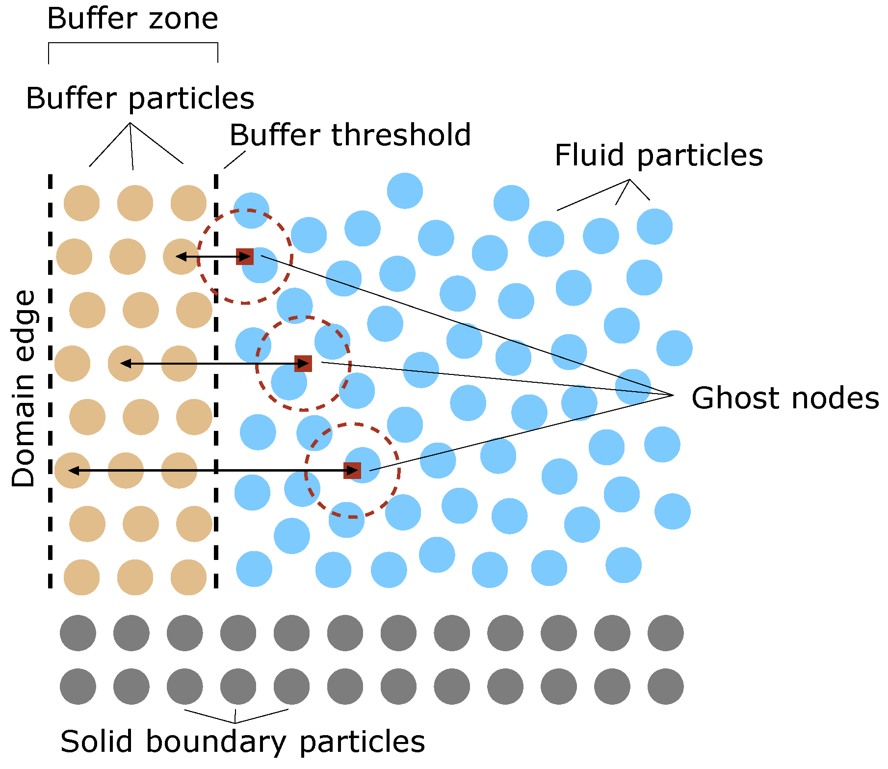
3.1. Open Boundary Conditions

The implementation of open boundaries in DualSPHysics is discussed in detail in Tafuni et al. [24]. Inflow and outflow buffer zones are defined near the inlets and outlets of the computational domain of DualSPHysics.

The implemented open boundary condition is illustrated in Figure 1, where a fluid is flowing near a buffer zone, implemented as an open boundary. The buffer zone is located in between the domain edge and the threshold boundary, which separates the fluid domain from the buffer zone. The buffer zone is filled with layers of SPH buffer particles on which boundary conditions can be imposed. The buffer size should be at least equal to or larger than the kernel radius. This is necessary to have full kernel support for the fluid particles close to the threshold boundary. In the present research, the buffer zone width is chosen as $8·d_p$ in the direction normal to the open boundary, where $d_p$ is the particle size adopted in DualSPHysics. There are two possibilities to provide physical information to the buffer particles: physical quantities are either imposed by the user or extrapolated from the fluid domain using so-called “ghost nodes”. As illustrated in Figure 1, the positions of the ghost nodes are calculated through mirroring of the buffer particle locations into the fluid domain, this along a direction which is perpendicular to the open boundary. When the fluid quantities are calculated at the ghost nodes, a standard SPH particle interpolation would not be consistent. Due to the proximity to an open boundary, the kernel would be truncated. Therefore, the method proposed by Liu and Liu [38] is applied to obtain first-order kernel and particle consistency. More specifically, a multi-dimensional, first-order Taylor series approximation of the field function $f(\mathbf{x})$ is multiplied by the kernel function evaluated at particle k, $W_k(\mathbf{x})$. The series approximation and its first order derivatives, $W_{k,\beta }(\mathbf{x})$, are given by:

$$\int f(\mathbf{x})W_k(\mathbf{x})d\mathbf{x}=f_k\int W_k(\mathbf{x})d\mathbf{x}+f_{k,\beta }\int (\mathbf{x}-{\mathbf{x}}_k)W_k(\mathbf{x})d\mathbf{x},$$

(10)

$$\int f(\mathbf{x})W_{k,\beta }(\mathbf{x})d\mathbf{x}=f_k\int W_{k,\beta }(\mathbf{x})d\mathbf{x}+f_{k,\beta }\int (\mathbf{x}-{\mathbf{x}}_{k,\beta })W_{k,\beta }(\mathbf{x})d\mathbf{x}.$$

(11)

Here, $\beta$ is an index ranging from 1 to $\delta$, the amount of dimensions. A system of $\delta +1$ equations in $\delta +1$ unknowns, $f_k$ and $f_{k,\beta }$ is formed. The solution to the system is given in particle notation:

$$f_k=\frac{\left|\begin{array}{cc}{\sum }_i{f}_i{W}_{ki}\mathsf{\Delta }{V}_i& {\sum }_i({\mathbf{x}}_i-{\mathbf{x}}_k)W_{ki}\mathsf{\Delta }{V}_i\\ {\sum }_i{f}_i{W}_{ki,\beta }\mathsf{\Delta }{V}_i& {\sum }_i({\mathbf{x}}_i-{\mathbf{x}}_k)W_{ki,\beta }\mathsf{\Delta }{V}_i\end{array}\right|}{\left|\begin{array}{cc}{\sum }_{i}f(\mathbf{x})W_{ki}\mathsf{\Delta }{V}_i& {\sum }_i({\mathbf{x}}_i-{\mathbf{x}}_k)W_{ki}\mathsf{\Delta }{V}_i\\ {\sum }_{i}f(\mathbf{x})W_{ki,\beta }\mathsf{\Delta }{V}_i& {\sum }_i({\mathbf{x}}_i-{\mathbf{x}}_k)W_{ki,\beta }\mathsf{\Delta }{V}_i\end{array}\right|},$$

(12)

$$f_{k,\beta }=\frac{\left|\begin{array}{cc}{\sum }_i{W}_{ki}\mathsf{\Delta }{V}_i& {\sum }_i{f}_i{W}_{ki}\mathsf{\Delta }{V}_i\\ {\sum }_i{W}_{ki,\beta }\mathsf{\Delta }{V}_i& {\sum }_i{f}_i{W}_{ki,\beta }\mathsf{\Delta }{V}_i\end{array}\right|}{\left|\begin{array}{cc}{\sum }_i{W}_{ki}\mathsf{\Delta }{V}_i& {\sum }_i({\mathbf{x}}_i-{\mathbf{x}}_k)W_{ki}\mathsf{\Delta }{V}_i\\ {\sum }_i{W}_{ki,\beta }\mathsf{\Delta }{V}_i& {\sum }_i({\mathbf{x}}_i-{\mathbf{x}}_k)W_{ki,\beta }\mathsf{\Delta }{V}_i\end{array}\right|}.$$

(13)

Next, the value of $f_o$ at the open boundary can then be found using the corrected values of $f_k$ and $f_{k,\beta }$ at the ghost nodes:

$$f_o=f_k+({\mathbf{r}}_o-{\mathbf{r}}_k)·\tilde{\nabla }{f}_k.$$

(14)

Here, $\tilde{\nabla }{f}_k$ is the corrected gradient at the ghost nodes.

The open boundary algorithm introduces several new features that make SPH more applicable to real engineering problems. The first one is the possibility of using buffer zones to impose time-varying velocity and pressure profiles, as well as pressure and velocity gradients along a specified direction. Next, a variable free-surface elevation can be imposed, which is an essential prerequisite in free-surface flow problems where waves can enter and exit the computational domain. Finally, the buffer zones are characterised by a dual behaviour, allowing both inward and outward flows, making flow reversion possible. Consequently, when flow velocities are extrapolated from the fluid domain, mixed velocity fields are possible where part of the buffer zone contains fluid particles entering the domain, and another part contains fluid particles leaving the domain. This can be specifically important in studying flow problems where modelling of strong rotations or oscillations is necessary. This flexibility is an important distinctive feature. The open boundary algorithm is available on both the parallel CPU and GPU versions of DualSPHysics. This results in considerable speed-ups when the code is running on powerful GPUs or large CPU clusters. This is particularly necessary when simulating real engineering problems. There, a large number of particles is required to simulate high-resolution flow problems with complex geometries, while maintaining a reasonable computation time.

3.2. Fixed Boundary Condition with Pressure Correction

Within DualSPHysics, fixed boundaries are normally realised using a set of particles called dynamic boundary particles [39]. These dynamic boundary conditions (DBC) have the advantage of being applicable to arbitrary 2D and 3D shapes, and provide good validation in many engineering problems. However, they are prone to unphysical fluid density and pressure values. Additionally, they exert high repulsive forces on the fluid particles, resulting in a separation distance. Within this work, a correction is applied to the dynamic boundary particles which resolves these issues. The DBC are here approached as a special case of an open boundary, more specifically one where the velocity of the buffer particles is zero, and the pressure is extrapolated from the fluid domain. This is similar to the approach by Marrone et al. [40]. The applied correction leads to less pressure oscillations in the fluid domain, and solves the occurrence of an unphysical gap between the boundary particles and the fluid. A downside of this method is the larger computation time, since both the continuity and momentum equations need to be solved for DBC and a unit vector, normal to the DBC, needs to be calculated for each boundary particle.

3.3. Comparison to the State-of-the-Art

A very similar implementation of the open boundaries presented in this work has been introduced by Ni et al. [25], as was already mentioned in the Introduction. This section explains the main differences to the open boundaries as implemented by Tafuni et al. [24] in more detail.

The main similarity between both methods is the use of buffer particles on which physical quantities such as velocity and surface elevation can be imposed. However, there are a few importance differences to be listed. Firstly, according to Ni et al. [25], the open boundaries are either an inlet or an outlet, while the implementation by Tafuni et al. [24] is more flexible and allows flow in both directions within one buffer zone. This makes it applicable to flow-reversion problems. Secondly, there are no ghost nodes to extrapolate physical quantities from the fluid domain to the buffer particles. Thirdly, the method to impose variable free surface in the buffer zone is different. Inter-particle distance is stretched out for fluctuations smaller than dp. When the necessary change is equal to or larger than dp, an extra row of particles is added. Here, the inter-particle distance in the vertical direction is kept constant, and a new row of particles is added when necessary. Fourthly, the applied active wave absorption at the inlet is similar to what is used in this work, but they impose a uniform incident velocity profile instead of correcting a variable profile with a uniform correction. Lastly, only first-order wave theory is used for the regular waves, as well as a simple solitary wave. The method presented here allows Stokes 5th order wave theory to be used as well as external input from OceanWave3D to produce accurate nonlinear waves.

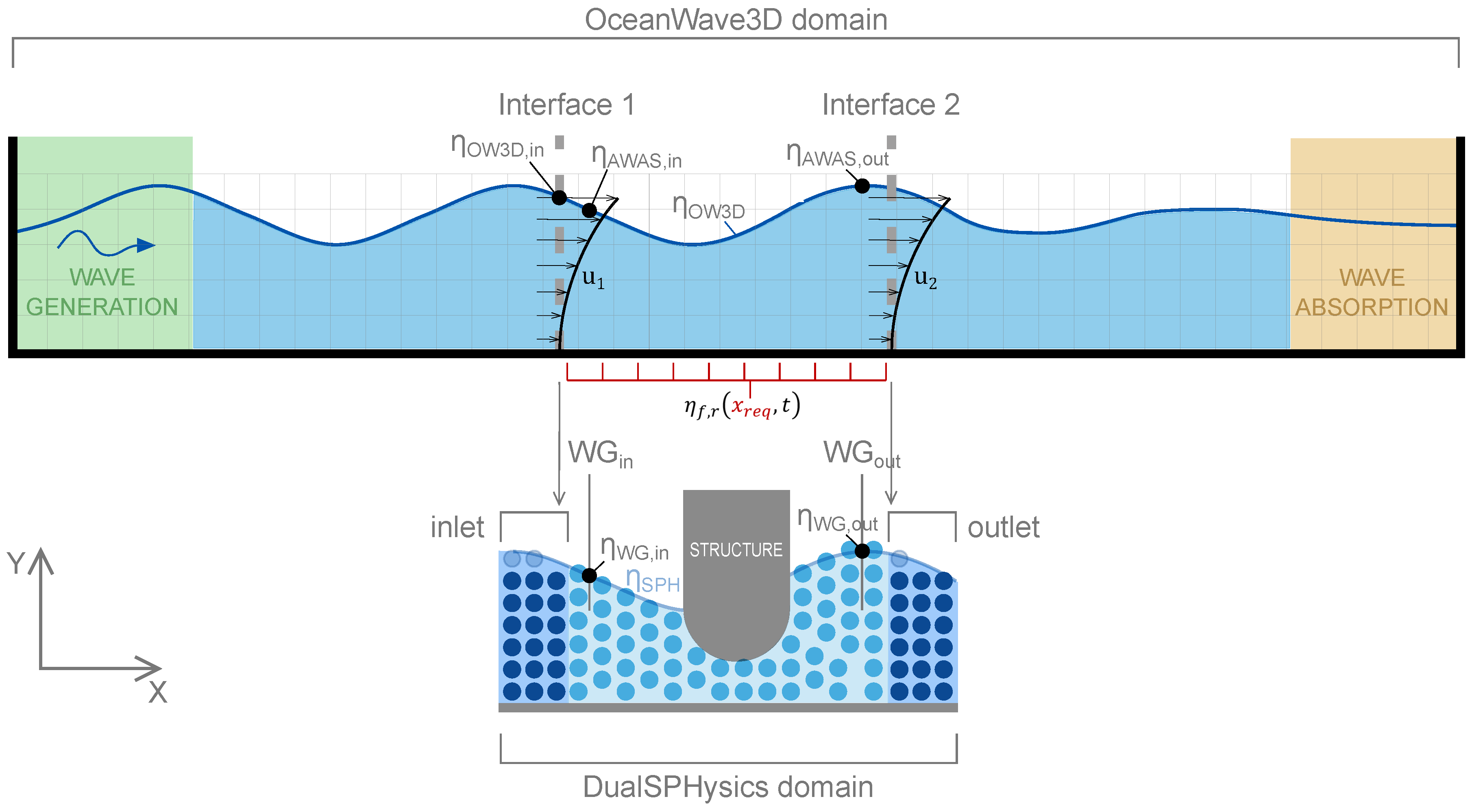
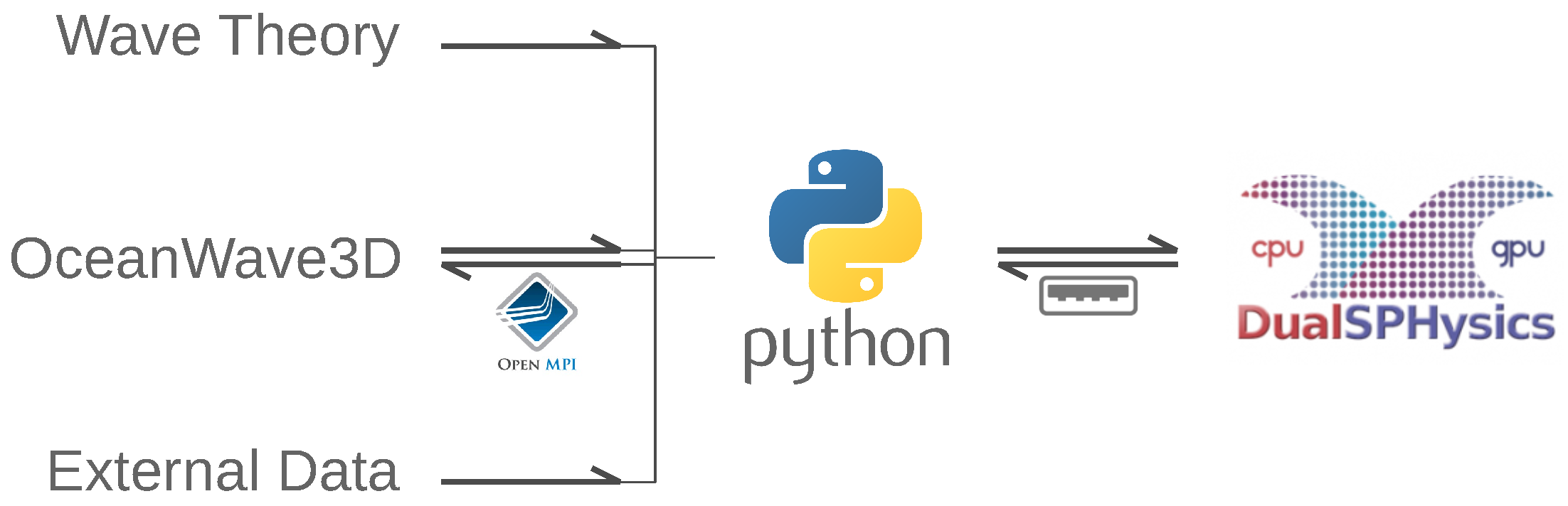
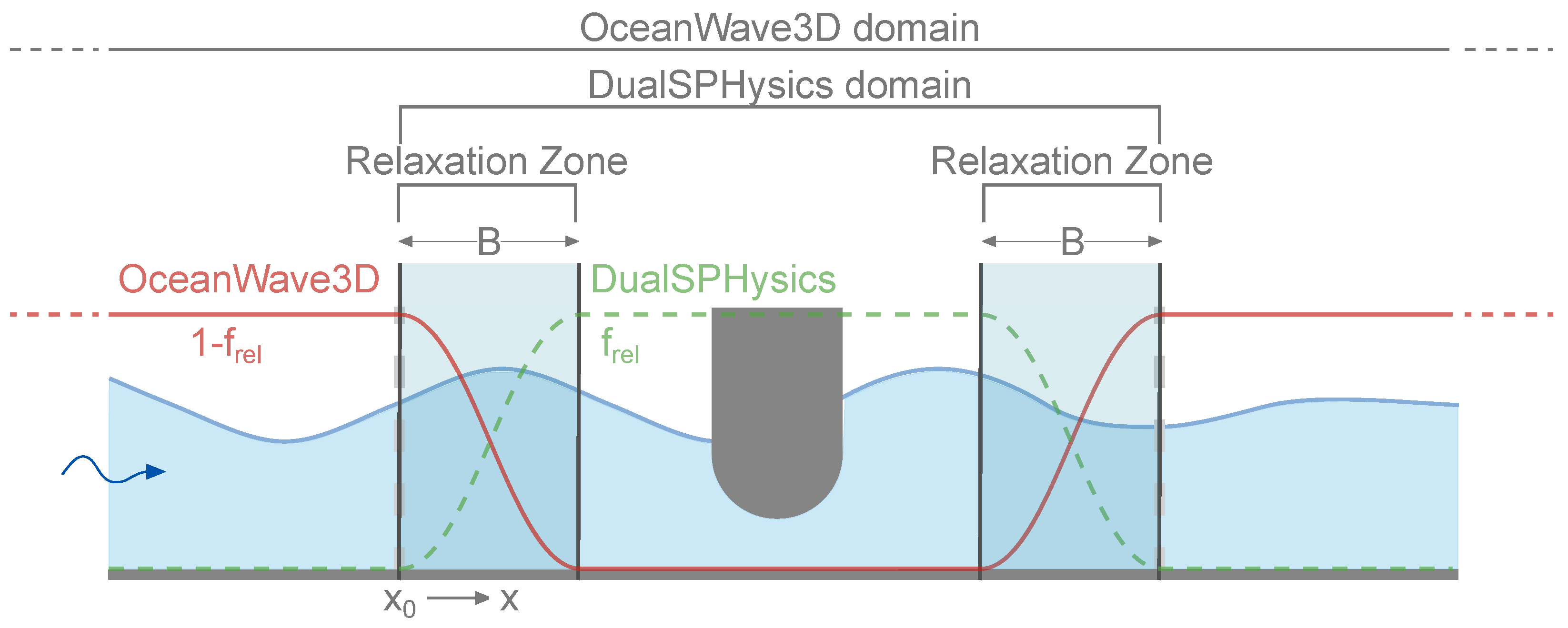
4. Coupling Methodology Using DualSPHysics and OceanWave3D

As mentioned before, SPH simulations are very computationally intensive. The flow and pressure fields required from a wave energy converter (WEC) SPH model are often limited to a zone closely spaced around the floating WEC. However, there is a spatial need to allow for proper wave generation and wave absorption, around 3–4 wavelengths long. This leads to a significant increase in water particles, and thus higher computation times. Moreover, wave generation techniques available in DualSPHysics are limited to first and second order wave generation by using piston-type or flap-type wave paddles. This generation type requires a certain propagation length before the full kinematics and surface elevation are developed. Within this research, the objective is to simulate higher-order (up to fifth-order) regular and irregular long-crested waves in a domain which is as small as possible. In an attempt to answer both the problem of computational performance and the problem of wave generation, a coupling methodology as illustrated in Figure 2 is developed.

Here, a DualSPHysics fluid domain with a length of one wave length $L_{wav}$ is chosen, with an inlet on the left-hand-side of the domain and an outlet on the right-hand-side of the domain (see Figure 2). Each buffer zone consists of eight layers of buffer particles. A sensitivity analysis illustrated in Figure 3 has shown that wave propagation results are accurate for buffer zones with at least eight layers. The dimensionless ratio $K_D=\frac{H_{measured}}{H_{imposed}}$, with H the wave height, is shown as a function of the normalized position $x/L_{wav}$ for a Stokes third-order wave. The number of buffer particle layers $n_l$ is varied from 1 to 16 and is doubled at each iteration.

The OceanWave3D domain is considerably larger and is often chosen as a multitude of wave lengths (e.g., 10). The wave generation zone measures around $2·L_{wav}$ while the wave absorption zone is taken as at least $3·L_{wav}$. The grid size $d_x$ is set as a multitude of the SPH inter-particle distance $d_x=n·d_p$. Here, n is set to be equal to 5. The physical quantities imposed on the SPH particle then originate from OceanWave3D. At the inlet, horizontal orbital velocities $u_1$ and surface elevation ${\eta }_{OW3D,in}$ originating from interface 1 are imposed on the buffer particles, while the pressure is set to be hydrostatic. At the outlet, only the horizontal orbital velocities $u_2$ originating from interface 2 are imposed, the surface elevation and pressure are extrapolated from the fluid domain (see

Table 1. Imposed and extrapolated quantities for inlet and outlet buffer particles (Imp = imposed, Ext = extrapolated, Hyd = hydrostatic).

Quantity	Horizontal Velocity u	Vertical Velocity w	Surface Elevation η	Pressure p
inlet	Imp	No	Imp	Hyd
outlet	Imp	No	Ext	Ext

). No vertical orbital velocities are applied, since there is no accuracy benefit by imposing vertical velocities, but there is a negative impact on stability, since the particle spacing increases vertically, leading to a reduced kernel support. To mitigate this problem, we managed to impose both horizontal and vertical velocities to the buffer particles, but only update the particle positions according to the horizontal velocities. However, no difference was noticed in the accuracy of the measured velocity fields and surface elevations. For this reason, only the horizontal orbital velocities were imposed.

By imposing horizontal velocities on both the inlet and outlet, the hydrodynamic problem becomes over-constrained, which can result in unwanted wave reflections in the fluid domain. Additionally, when a floating or fixed structure is positioned in the fluid domain, waves will reflect on the structure and transform around it. The open boundaries should be able to compensate for the reflected waves and the outlet needs to absorb the transformed wave effectively. In this research, this is done by applying velocity corrections at the inlet and the outlet, based on the measured free surface close to the buffer zones, specifically at a distance of $8·d_p$. This distance has been selected based on a sensitivity analysis, illustrated in Figure 4. The same Stokes third-order wave was simulated, each time varying the wave measurement distance $d_{WG}$ from $1·d_p$ to $16·d_p$. For a value of $d_{WG}$ equal to $8·d_p$, the wave measurement location is close enough to the buffer zone to have a minimal phase difference, but far enough to avoid inaccuracies due to transitional effects between the buffer zone and the fluid domain. In Figure 2, these measuring locations are denoted as $W{G}_{in}$ (Wave Gauge) and $W{G}_{out}$. The applied velocity correction is a shallow water wave correction based on the measured reflection [41], but is implemented differently depending on the inlet or the outlet.

4.1. Inlet Velocity Correction

At the inlet, the objective is to generate always the required incident wave. The surface elevation is measured directly outside of the inlet, and the velocity is corrected to ensure that the generated surface elevation matches the theoretical one. In case a higher surface elevation is measured than what was imposed, the corrected velocity should be lower than the originally imposed profile, in order to compensate the excess of velocity, since that profile leads to wave reflections in the fluid domain. Within the code, this correction is implemented as follows:

$$\begin{array}{c}\hfill u_{in}(z,t)=u_1(z,t)-\left[{\eta }_{WG,in}-{\eta }_{AWAS,in}\right]·\sqrt{\frac{g}{d}}.\end{array}$$

(15)

Here, $u_{in}$ is the horizontal velocity at the inlet, $u_1$ is the imposed horizontal velocity coming from OceanWave3D, ${\eta }_{WG,in}$ is the measured free surface elevation near the inlet, ${\eta }_{AWAS,in}$ is the OceanWave3D free surface measured at the location of $W{G}_{in}$, g is the earth’s acceleration and d is the water depth. This correction is similar to the active wave absorption applied in Altomare et al. [42], although there it was used to correct the displacement of a piston-type wave maker formed by moving boundary particles instead of buffer particles.

4.2. Outlet Velocity Correction

At the outlet, the objective is to absorb any wave propagating towards the outlet. Technically, the applied open boundaries do not absorb the waves, but rather try to match the velocity field present in the fluid domain as close as possible, creating an ’open door’ for the propagating wave. The surface elevation ${\eta }_{WG,out}$ is measured directly outside of the outlet, and compared to the calculated OceanWave3D free surface ${\eta }_{AWAS,out}$ at the location of $W{G}_{out}$. The velocity $u_{out}$ is then corrected to ensure that the imposed velocities $u_2$ match the measured ones. In case a higher surface elevation ${\eta }_{WG,out}$ is measured than what was imposed ${\eta }_{AWAS,out}$, the corrected velocity $u_{out}$ should be higher than the originally imposed velocity $u_2$. Otherwise, discontinuities in the velocity field would occur, which would induce unwanted reflected waves into the domain:

$$\begin{array}{c}\hfill u_{out}(z,t)=u_2(z,t)-\left[{\eta }_{AWAS,out}-{\eta }_{WG,out}\right]·\sqrt{\frac{g}{d}}.\end{array}$$

(16)

4.3. Coupling Algorithm

The implementation of the coupling is illustrated in Figure 5. The detailed wave–structure interactions are calculated with the latest version of DualSPHysics (v4.2.030). As mentioned in Section 4, velocity corrections need to be applied for accurate representation of the free-surface elevation and the wave kinematics. For this reason, a two-way coupling is realised between a Python [43] program and DualSPHysics. Rather than a direct coupling between OceanWave3D and DualSPHysics, Python is used as an intermediate communication step. This allows for the coupling to be more generic, and not exclusively applicable to OceanWave3D. Additionally, the use of Python allows the user to monitor the simulation and easily perform accuracy checks on the transferred data. The Transmission Control Protocol (TCP) is used for the data transfer. At the start of the simulation, a dedicated port (50007) is opened to allow communication. At the start of each time step, Python sends both the inlet and outlet velocities and the inlet surface elevation to DualSPHysics. At the end of the time step, DualSPHyics sends back the measured surface elevation near the inlet and outlet. In Python, the velocity corrections are calculated and applied to the originally imposed horizontal velocities. With this coupling methodology, any data can be used to impose horizontal velocities and surface elevation to the inlet and outlet buffer zones. For example, wave theory solutions are an excellent method to provide the model with accurate orbital velocities and surface elevations. Alternative to using wave theory, and as demonstrated in this paper, the wave propagation model OceanWave3D can be coupled to DualSPHysics using the MPI protocol for data transfer. Here, the use of a TCP port was not possible due to compatibility issues with the OceanWave3D Fortran code. Although the coupling methodology is here specifically introduced for ocean wave simulations, it can be generalised to a more generic application. Specifically, the implementation using Python as an intermediate communication process, and using TCP sockets and the MPI protocol to send data from one software package to another, can be applied to other research domains as well. For example, an open channel flow modelling tool can be coupled to SPH to simulate river flow dynamics, or a 1D pipe flow hydraulic model can be coupled to SPH to simulate pressurized flow problems. However, a detailed study of the applicability of the methodology falls outside the scope of this research.

Apart from the implementation, a schematic representation of the coupling algorithm is illustrated in Figure 6. The most complex coupling is discussed here, being the two-way coupling with OceanWave3D. The coupling communication occurs at the beginning and at the end of an OceanWave3D time step, which is referred to as the “communication time step”. Due to the larger grid size and simplified equations in OceanWave3D, the communication time step is considerably larger than the DualSPHysics time step. This means that DualSPHysics performs multiple smaller time steps during one communication time step. At the beginning of a communication time step, the horizontal orbital velocities at the inlet and outlet locations, $u_1$ and $u_2$, are calculated in OceanWave3D, as well as the surface elevation of the complete OceanWave3D domain ${\eta }_{OW3D}$, and sent to the Python programming using the MPI protocol. Simultaneously, Python receives the measured surface elevation from DualSPHysics near the inlet and outlet ${\eta }_{WG,in/out}$. The velocity correction is calculated using ${\eta }_{AWAS,in}$ and ${\eta }_{AWAS,out}$, resulting in the corrected orbital velocities $u_{in/out}$ which are sent back to DualSPHysics, together with the surface elevation at the inlet ${\eta }_{OW3D,in}$. The quantities are imposed within the inlet and outlet buffer zones and the DualSPHysics simulation calculates multiple time steps until the communication time step is reached. The surface elevation from DualSPHysics ${\eta }_{SPH}$ is sent to Python, where the signal is filtered and sent back to OceanWave3D as ${\eta }_{f,r}$ to overwrite the original result. To ensure a smooth transition between the DualSPHysics free surface and the OceanWave3D free surface, a relaxation functions $f_{rel}$ is applied (see Figure 7). The applied function $f_{rel}$ is the same as is applied within OceanWave3D’s generation and absorption relaxation zones. Within the relaxation zone, the filtered solution ${\eta }_{f,r}$ is then obtained as given in Equation (18), with B the length of the zone, x the location within the relaxation zone and $x_0$ the reference location of the relaxation zone:

$$\begin{array}{ccc}\hfill {\eta }_{f,r}& =& (1-f_{rel})·{\eta }_{OW3D}+f_{rel}·{\eta }_{SPH},\hfill \end{array}$$

(17)

$$\begin{array}{ccc}\hfill f_{rel}& =& {\left(\frac{x-x_0}{B}\right)}^{3.5}.\hfill \end{array}$$

(18)

5. 2D Coupled Model: Validation

First, the two-way coupling between DualSPHysics and OceanWave3D is validated in 2D. The coupling is applied to compare the response of a box, floating in three degrees of freedom (heave, surge and pitch) to experimental data, as described in Ren et al. [44]. The numerical test set-up is illustrated in Figure 8. The full OceanWave3D domain has a length of 20.0 m, while the DualSPHysics domain is 6.12 m long (three wave lengths) and starts at $x=4.0$ m. The floating box is positioned at $x=5.5$ m in a water depth of $d=0.4$ m and has the dimensions 0.3 m × 0.2 m (length × height) with a draft $q_{box}=0.1$ m. A regular wave with wave height $H=0.1$ m and wave period $T=1.2$ s is generated, characterised as a Stokes third-order wave. A particle size of $d_p=0.01$ m is used. The SPH domain is chosen to be larger than one wavelength $L_{wav}$, since the box is freely floating and will drift in the x-direction over time.

5.1. DualSPHysics Solver Options

The efficiency and accuracy of DualSPHysics was investigated in Altomare et al. [45] for wave propagation and absorption showing good agreement between numerical results and experimental data. Accordingly, similar DualSPHysics solver options used for that work will be used here to perform the numerical simulations. The solver options used in this section are summarized in

Table 2. SPH formulation and parameters.

Time Integration Scheme	Verlet
Time Step	Variable (including CFL and viscosity)
Kernel	Wendland
Smoothing Length	$2.0·d_p$
Viscosity Treatment	Artificial ($\alpha =0.01$)
Equation of State	Tait equation
Boundary Conditions	Open Boundary Conditions
$\delta$-SPH	Yes ($\delta$-SPH = 0.1)

. The time integration scheme is chosen to be the Verlet scheme, employing a variable time step based on the CFL number. The chosen kernel is the Wendland kernel with a smoothing length of $h_{SPH}=2.0·d_p$. The artificial viscosity is set to be $\alpha =0.01$. Tait’s equation of state is applied to calculate the fluid pressures. The boundary conditions are the open boundaries introduced by Tafuni et al. [24] and some numerical diffusivity is added by applying a $\delta$-SPH treatment with a coefficient of $\delta -SPH=0.1$. These parameters have been thoroughly studied in Verbrugghe [46] and have proven to lead to accurate wave propagation within DualSPHysics. There, a convergence analysis has proven a convergence rate in between first-order and second-order, and a thorough validation study of the wave dynamics was performed.

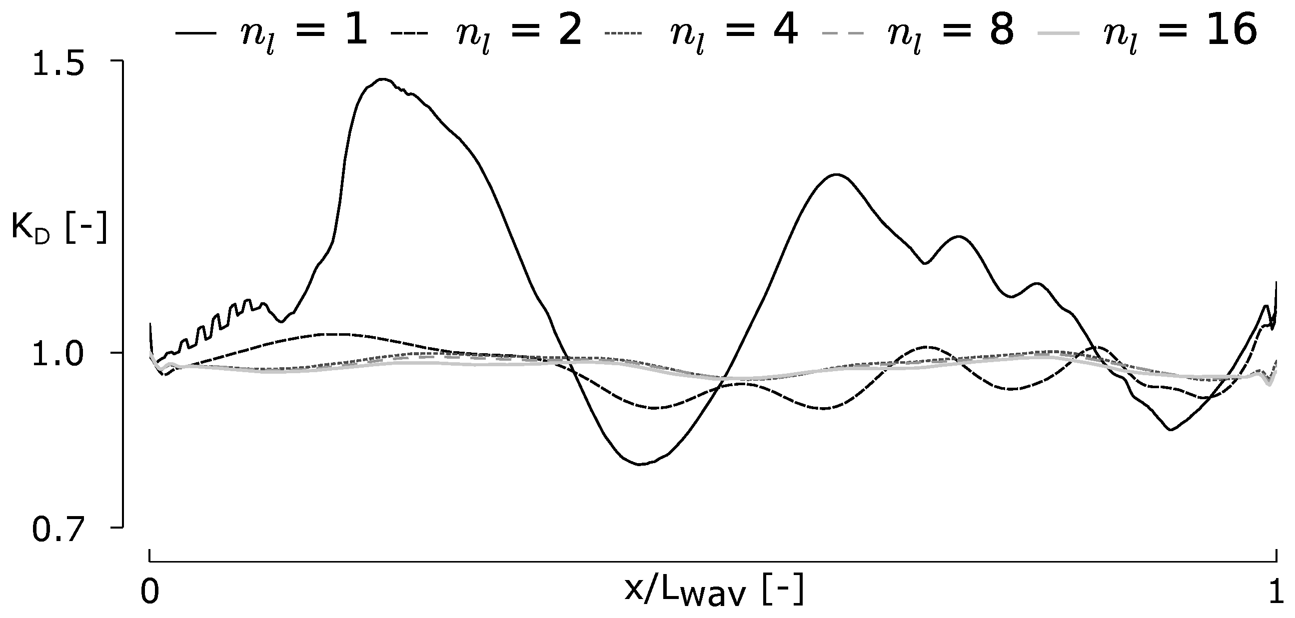
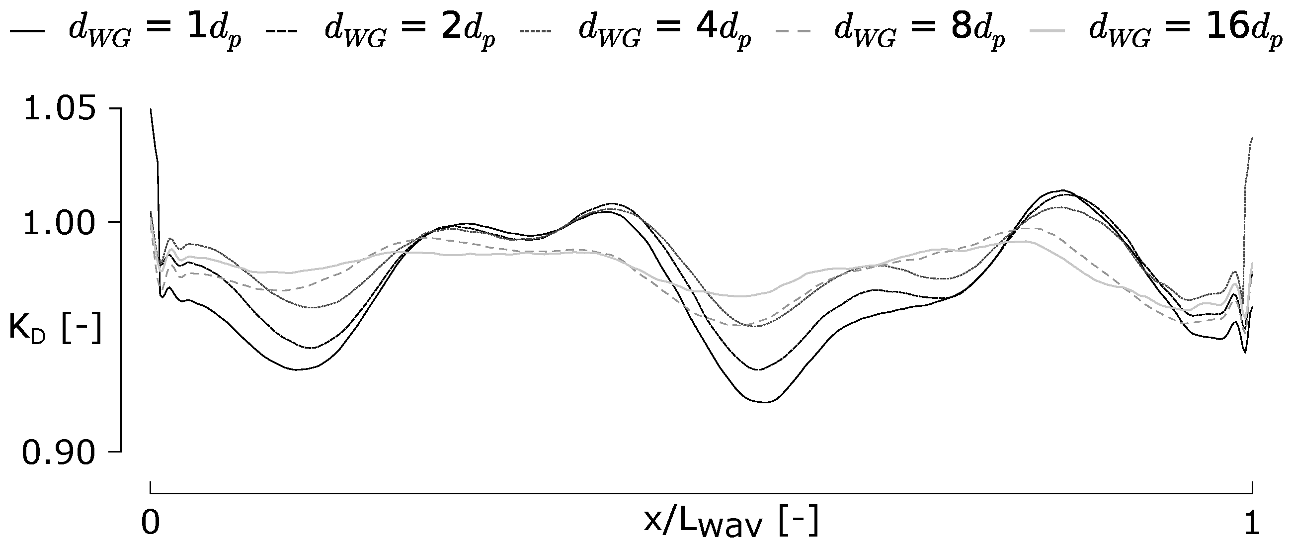
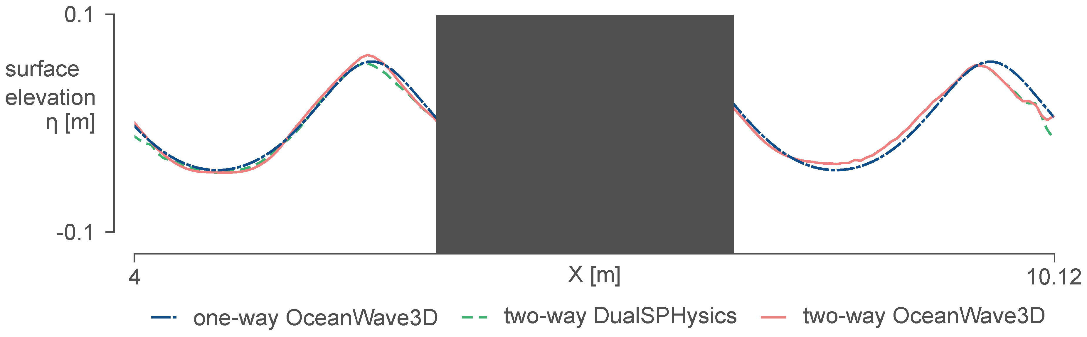
5.2. Results and Discussion

Both a one-way coupling and two-way coupling are compared to the experimental data, and the corresponding errors are illustrated in Figure 9. In the one-way coupling, OceanWave3D only provides the horizontal orbital velocities to the inlet and outlet zone, and the surface elevations for the inlet and the calculation of the velocity corrections. For the two-way coupling, the surface elevations from the DualSPHysics domain are transferred back to the OceanWave3D domain, where the original solution is overwritten. The part close around the floating box is not coupled back, since the ’measured’ SPH free surface elevations are not physical there. The top three graphs of Figure 9 show a direct comparison between the experimental and numerical results for the heave motion, the pitch motion and the surge motion, respectively. Qualitatively, a good correspondence between the numerical and experimental results is shown. Specifically, the heave and pitch motions are accurately reproduced. In order to quantify the accuracy of the results, the difference between the experimental and numerical results is calculated and illustrated in the bottom three graphs of Figure 9. The error on the heave motions remains well below the smoothing length $h=0.02$ m. Additionally, it can be noticed that the result from the two-way coupling has a lower error than the result from the one-way coupling. The pitch error stays below 3.5 degrees, which is around $10\%$ of the total pitch motion range, and there is no clear distinction in the error between the one-way coupling and the two-way coupling. The error on the surge motion is less satisfactory. Here, both the one-way coupling and two-way coupling are less capable of modelling the cyclic surge path, the net drift in the x-direction is even less accurate for the two-way coupling as for the one-way coupling. However, since the error on the surge motion logically becomes larger in time, the results are still acceptable.

Additionally, the instantaneous surface elevation profile at $t=15$ s of DualSPHysics and OceanWave3D is compared in Figure 10. Here, the part close to the floating box is masked out since there is no coupling performed there. Three surface elevation profiles are plotted. For the two-way coupling methodology, both the OceanWave3D and DualSPHysics profile are plotted. Normally, these lines are expected to be exactly the same, since the original OceanWave3D surface elevation is overwritten. However, relaxation functions are applied to ensure a smooth transition between the OceanWave3D solution and the DualSPHysics solution. In Figure 10, this can be noticed close to the masked out zone both solutions match perfectly. Behind the masked-out zone, both solutions remain the same until they slightly differ again at the boundary of the SPH zone ($x=10.12$ m). As a reference, the OceanWave3D solution for a one-way coupling is shown as well. Here, there is no influence from the DualSPHysics solution, and OceanWave3D propagates waves as if there is no floating box present. Nevertheless, this does not impact the accuracy of the results significantly, as proven in Figure 9. In general, it can be concluded that the one-way coupling is slightly more accurate than the two-way coupling. The advice is to only apply the two-way coupling methodology, when there is a significant wave transformation effect around the structure, which needs to be propagated further within the larger OceanWave3D domain. For example, modelling a WEC device that extracts a significant amount of energy from the waves will result in a significant reduction of wave height behind the device. When it is required to model the further propagation of that reduced wave within the larger OceanWave3D domain, a two-way coupling should be applied. Otherwise, when there is no interest in the wave field, far away from the DualSPHysics domain, the one-way coupling is advised.

6. 3D Coupled Model: Proof-of-Concept

In this section, the introduced coupling methodology is extended to a 3D domain. A one-way coupling with a fifth-order Stokes wave theory is applied. The buffer zones are stretched in the y-direction, perpendicular to the 2D plane of the 2D validation case, and the imposed quantities are constant in that y-direction. This means 3D simulations are restricted to long-crested waves. Consequently, the coupling methodology can be used to model wave flume type experiments where significant 3D effects are present. To demonstrate this, a heaving disk is simulated, impacted by steep nonlinear waves. This results in nonlinear wave surge forces and wave overtopping.

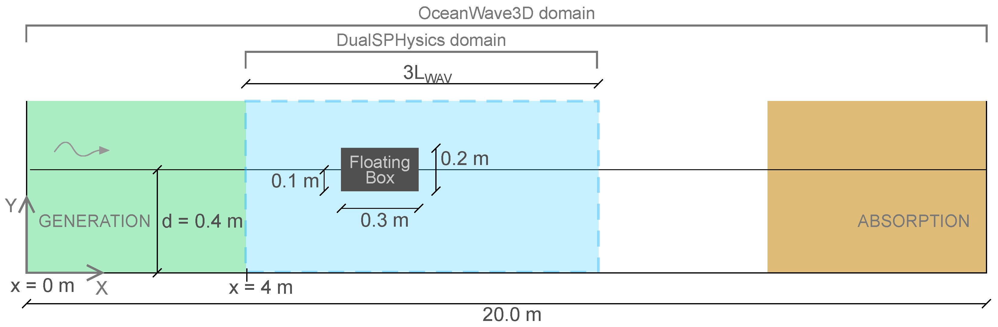
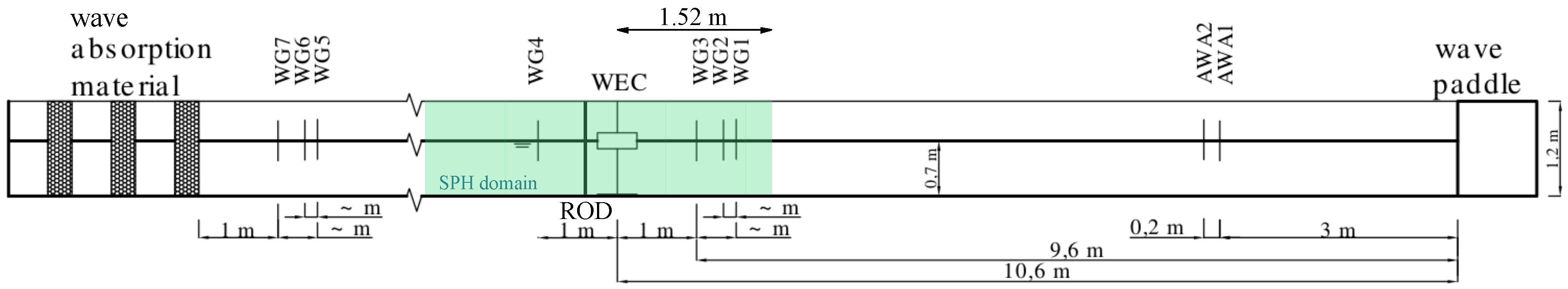
6.1. Experimental Set-up

Experiments have been performed in the large wave flume of Ghent University (see Figure 11). The flume is 30.0 m long and 1.0 m wide. A cylindrical WEC with a diameter of $D=0.5$ m is positioned at a distance of 10.6 m from the wave paddle. The WEC’s motion is restricted to heave by a vertical rod over which it is sliding. Friction losses are minimized by using two sets of PTFE bearings: one on the top and one on the bottom of the cylinder. The WEC consists of 10 glued plastic disks and is waterproofed with a black, silyl-modified (MS) polymer coating. Wave absorption material is installed at the left end of the wave flume to ensure minimal wave reflections. Active wave absorption is applied using two wave gauges about 3.0 m away from the wave paddle. Seven wave gauges (WG) are installed to measure the free surface elevation. The WEC has a draft of $q_{WEC}=0.113$ m. The motion of the WEC is captured by video tracking using a GoPro Hero 5 [47], filming in Full HD at 120 fps. The typical fisheye distortion is corrected using video processing software. The horizontal surge force $F_{x,WEC}$ is measured by 2 force transducers, installed in a rigid rod behind the WEC to which it is connected. The incident wave has a wave height of $H=0.12$ m, a wave period of $T=1.2$ s in a water depth of $d=0.7$ m. This results in a Stokes third-order wave with a wave length of $L_{wav}=2.17$ m.

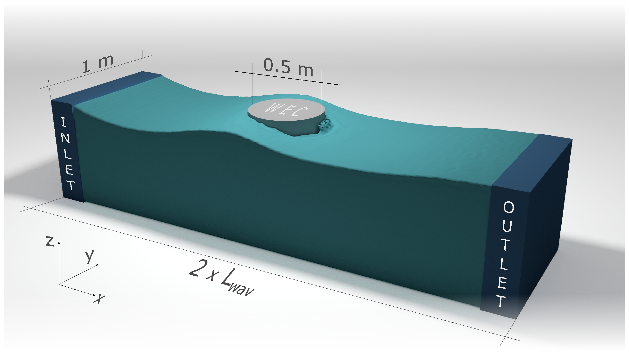
6.2. Numerical Set-up

The numerical set-up is illustrated in Figure 12 and summarized in

Table 3. Simulation parameters for 3D modelling of a heaving cylindrical WEC.

Wave Height H [m]	0.12
Wave Period T [s]	1.2
Water Depth d [m]	0.7
Wave Length L${}_{wav}$ [m]	2.17
Particle Size d${}_p$ [m]	0.01
Domain Length $L_{SPH}$ [m]	4.34
Domain Width W [m]	1.0
WEC Diameter D [m]	0.5
WEC Draft q${}_{WEC}$ [m]	0.113
Wave Theory	Stokes 5th
Time Step Algorithm	Verlet
Artificial Viscosity	0.01
$\delta$-SPH	0.1

. It is chosen to set the length of the fluid domain to twice the wave length $L_{SPH}=2·L_{wav}=4.34$ m. This is around $1/7$ of the total flume length. The particle size is chosen to be $d_p=0.01$ m. The Stokes fifth-order wave theory is applied. Since there is always a gap of 1.5 times the smoothing length $h_{SPH}$ between fluid particles and boundary particles, the top of the floating disk is lowered with a value of $1.5·h_{SPH}=1.5·2.0·d_p$, in order to get the correct wave overtopping height. A 3D inlet zone and outlet zone are configured, with each eight layers of buffer particles. All other boundaries are fixed boundary conditions with the option to extrapolate the pressure from the fluid domain, in order to avoid local pressure peaks (see Section 3.2). The WEC is positioned at a distance of 1.52 m from the inlet boundary of the numerical domain.

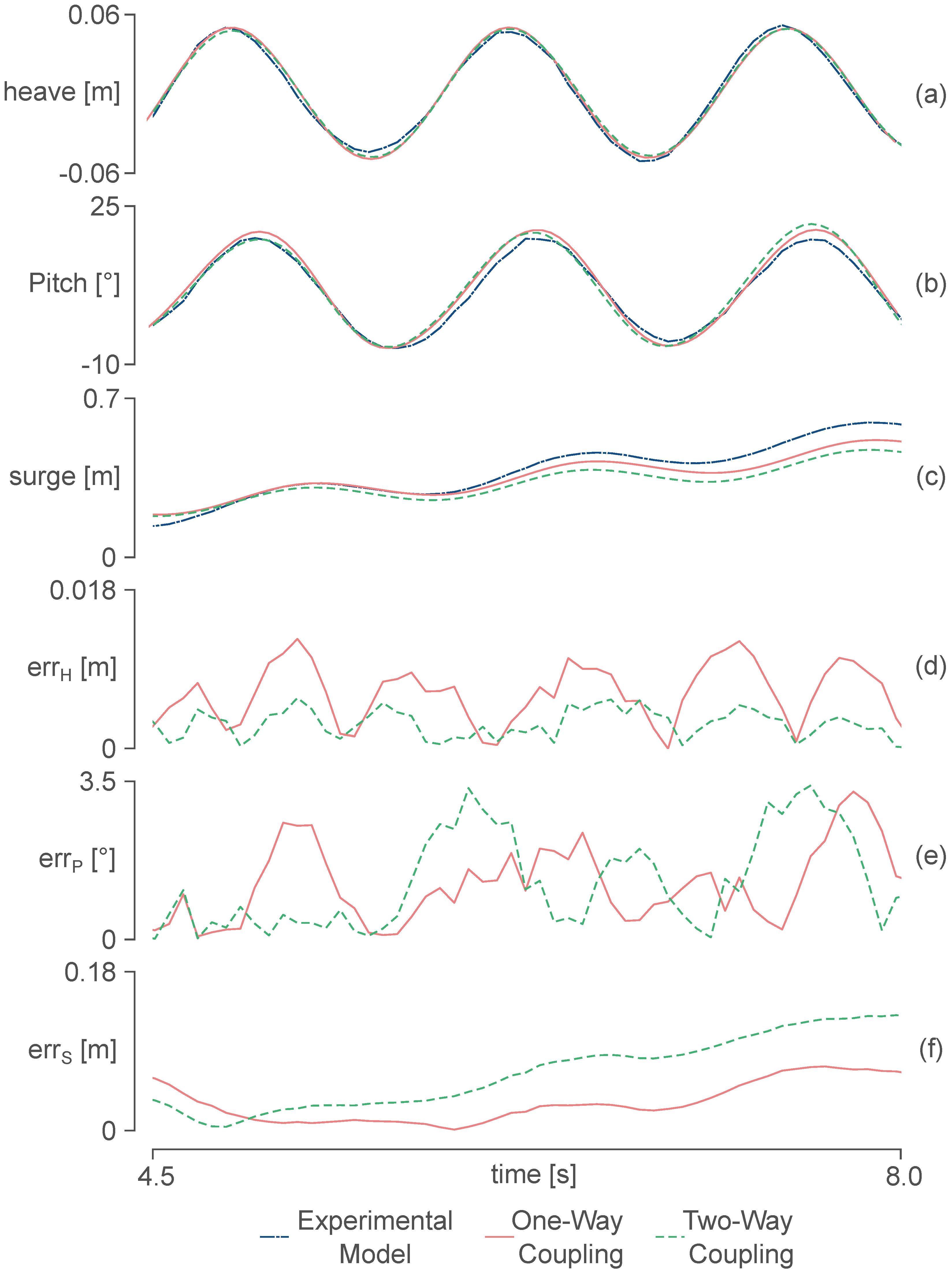
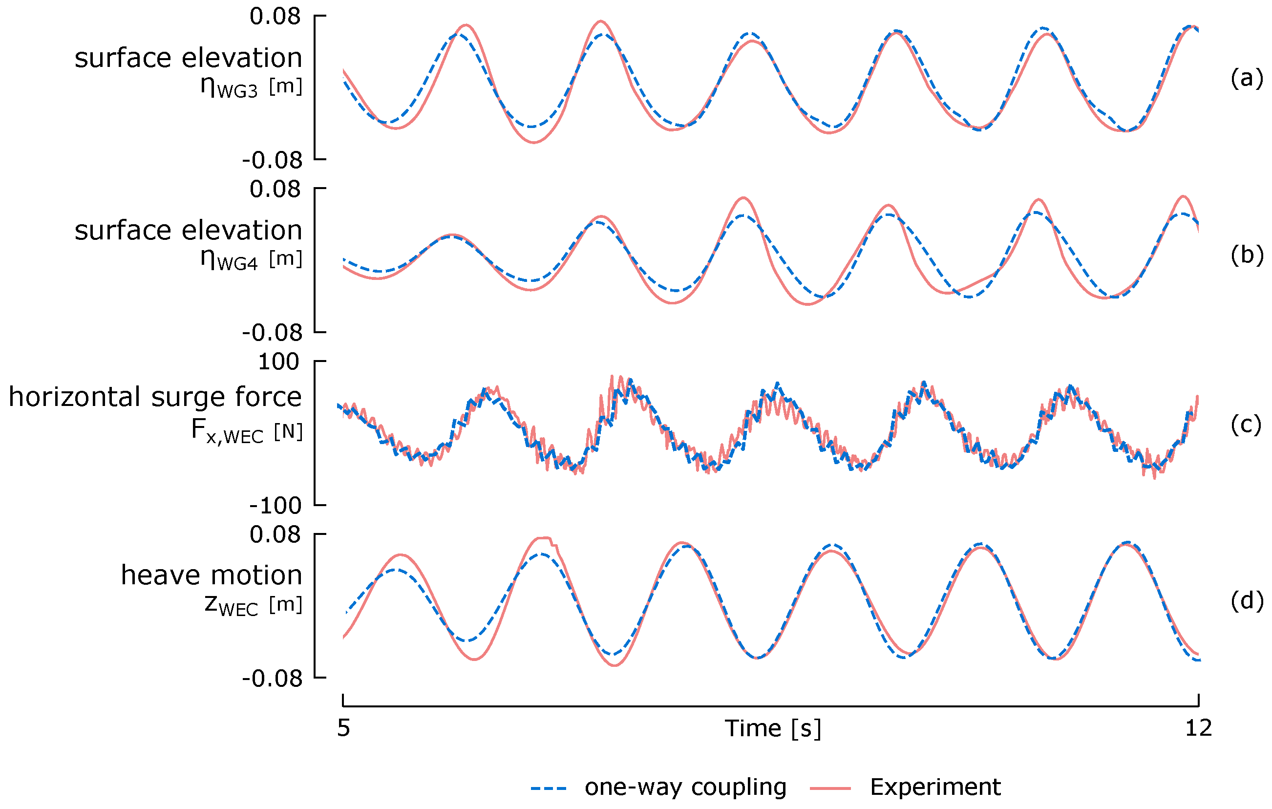
6.3. Results and Discussion

First, the numerical surface elevations from the one-way coupled model are compared with experimental results. The signals from WG3 and WG4 (see Figure 11) are compared to the numerical results. WG3 is positioned 1.0 m in front of the WEC, WG4 1.0 m behind the WEC. The comparison with the data from WG3 is shown in plot (a) of Figure 13, while plot (b) shows the comparison with the WG4 data. The surface elevation in front of the WEC is accurately reproduced. There is some initialisation time, but after a while the wave signal is steady and matches the experimental data very well. The error remains well below the smoothing length $h_{SPH}=0.02$ m. Behind the WEC, the numerical results are less accurate. The one-way coupled model calculates lower wave heights behind the WEC than what was registered in the experiments. The measured free surface also has a steeper nonlinear profile than what was calculated numerically. This could be due to the shortened SPH domain with respect to the full experimental wave flume length. However, the error on the surface elevation is still acceptable since the maximum error at the third wave crest measures 0.0196 m and is still smaller than the smoothing length $h_{SPH}$.

Second, the horizontal surge force is calculated and compared to the experimental data in plot (c) of Figure 3. Here, it is clear that there is a very good match between the numerical and experimental results. Although both signals have some noise, the overall trend of the data matches very well.

Third, the comparison of the heave motion of the WEC to the experimental data is shown in plot (d) of Figure 3. Again, after initialisation of the surface elevation in the wave flume, a steady regime is obtained in which the calculated WEC motion and measured motion show an excellent agreement, with a maximum error of $0.4h_{SPH}$.

6.4. Computational Speed-up

The coupling methodology with open boundaries leads to significant performance gains with respect to typical SPH simulations. In this section, an estimation of the computational speed-up is made, comparing the presented one-way coupled model with a stand-alone numerical model, describing the complete experimental set-up. The latter is thus an SPH simulation where the full wave flume is modelled, including the wave paddle motion and the floating disk, installed at $x=10.6$ m. The comparison is summarized in

Table 4. Computational speed-up for 3D proof-of-concept.

	One-Way Coupling	Full Model	Difference
# Particles	5,010,954	25,473,152	508%
# Fluid Particles	2,949,433	21,165,100	718%
GPU Memory [MB]	780	3941	505%
Estimated Runtime [hr]	35	144	411%
Real Runtime [hr]	91	375	411%

. In the one-way coupled model, the domain length was set at twice the wave length, resulting in a total length of 4.34 m. This is about 1/7 of the wave flume length, which explains the number of fluid particles in the full model, which is about 718% more than in the one-way coupled model. The difference in total number of particles is lower, at only 508%. This is due to the thickness of the bottom boundary in the coupled model, which is thicker to allow for accurate pressure extrapolation. The difference in GPU memory is similar at 505%, with an absolute value of 3941 MB for the full model. Although our GPU card has 8106 MB of memory available, this simulation is incredibly demanding. Computational performance is not only dependent on GPU memory, since the number of CUDA cores and their clock rate are much more indicative of simulation time. The estimated runtime, which is calculated at the start of the simulation, is significantly longer for the full model than for the coupled model. However, the difference of 411% is slightly lower than the difference in particles. The real runtime of the coupled model was 91 h. This remarkable difference in estimated runtime and real runtime can be explained by inaccurate estimations at the beginning of the simulation, in combination with performing other tasks on the computer, slowing down the simulation. It is chosen to not run the full model completely, since the computer becomes unusable during the simulation and it could take up to 375 h or almost 16 days to finish if the same performance as the coupled model is assumed. It is safe to assume that a speed-up of around 400% can be achieved, by applying the coupling methodology.

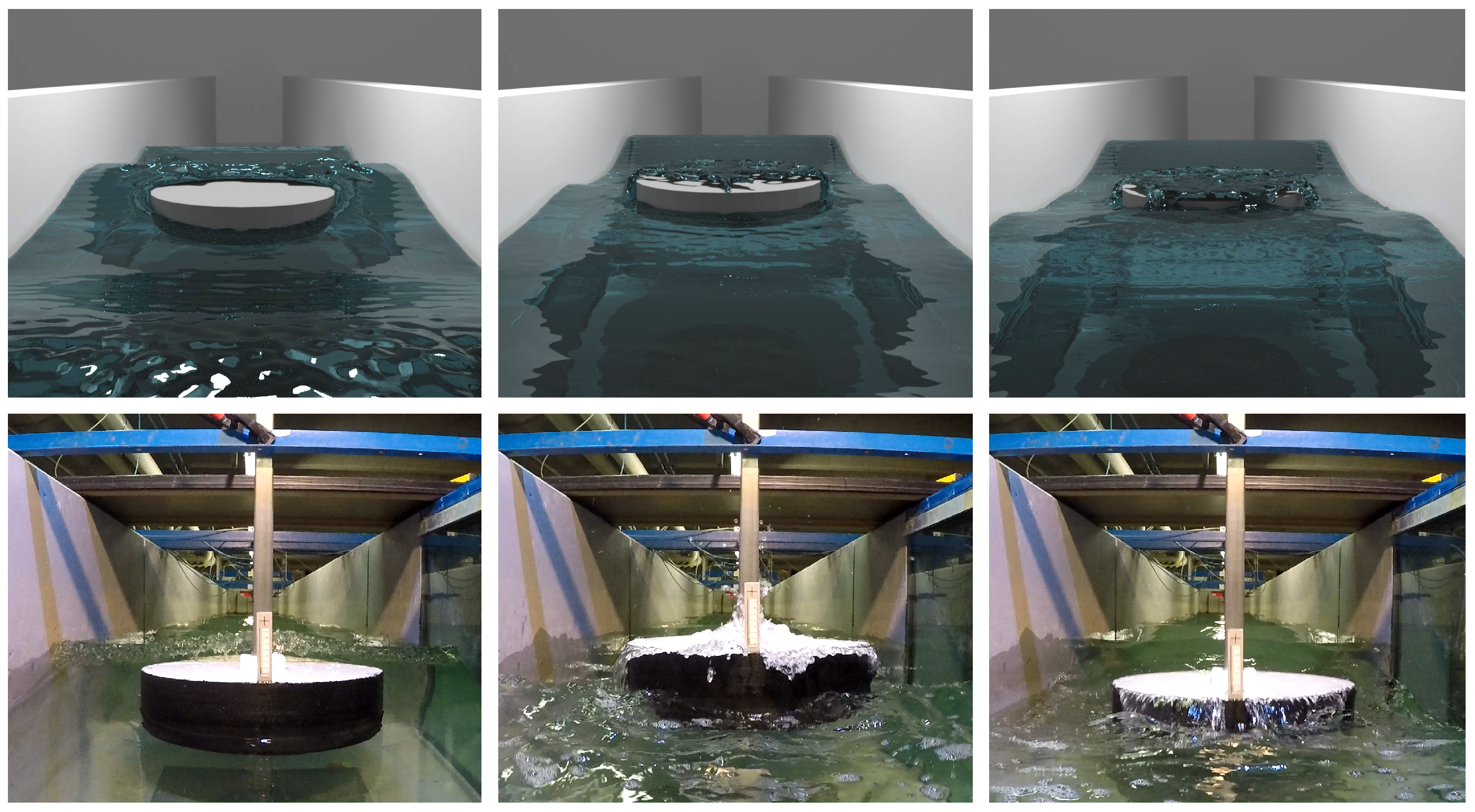
6.5. Visual Comparison of Overtopping

During the experiments, some of the steep nonlinear waves were overtopping the cylindrical WEC. However, no overtopping rates or thickness of the overtopping layer were measured, so a correct validation is not possible. For this reason, only a visual comparison of an overtopping event between the experiment and the numerical model is performed. In Figure 14, a time progression of an overtopping wave is shown. Here, the wave height was set at $H=0.15$ m and the wave period was $T=1.0$ s. This resulted in steep, highly nonlinear waves with significant overtopping. In addition, for this test case, video images were available to perform a visual comparison. In the left plot, the wave is just about to hit the cylindrical WEC. In the middle plot, 0.4 s later, the overtopping wave is on top of the WEC, and in the final plot, the overtopped volume is flowing from the top back into the flume. Visually, the correspondence between the numerical model and the experimental images is very good, apart from the interactions of the overtopped water with the vertical rod, since the rod was not included in the numerical model.

7. Conclusions

Development of accurate boundary conditions and the coupling of SPH solvers to external models are identified as key topics within the SPHERIC Grand Challenges to let SPH method attain a high level of maturity. The present work is a clear contribution to both issues, proposing a novel two-way coupling methodology that applies the open boundary formulation to accurately generate, propagate and absorb waves within a two-way coupled DualSPHysics-OceanWave3D model. A Python program was used as an intermediate process to calculate and apply the velocity corrections to the inlet and outlet buffer zones, to avoid reflections inside the DualSPHysics fluid domain. This coupling technique allows overcoming one of the main shortcomings of SPH-based solvers, related to computational cost. Despite the increase of HPC and GPU performance during the last years, a large number of particles (i.e., high model resolution) is still necessary, in order to simulate real engineering problems with sufficient accuracy. A coupling between a detailed but computationally expensive mesh-free model and a wave propagation model represents a trade-off between model accuracy and efficiency. This can be done by coupling SPH to a faster external numerical model which can deal easily with large computational domains. A proper two-way coupling scheme, however, requires accurate and stable boundary conditions. In fact, a reduced domain size is useless when the imposed quantities at the boundary are not accurate enough. Through coupling, other software packages (fast-calculating) can be applied to provide physical quantities to the boundary conditions, more accurately than what the built-in methods or analytical solutions can provide. The two-way coupling methodology with OceanWave3D was validated in 2D by comparing the surface elevations and the motions of a floating box to experimental data. Finally, a 3D proof-of-concept was introduced where steep nonlinear waves interact with and overtop a heaving cylindrical WEC. The results all show a good agreement with the experimental data. In the performed tests, the coupled model has at least two to four times less particles to simulate, which directly results into faster computation times. Alternatively, for the same computation time as a stand-alone SPH simulation, there is the possibility of simulating more particles for a higher accuracy. One of the main benefits of using open boundary conditions rather than moving boundaries or relaxation zone techniques is that there are no issues with Stokes drift, and the velocity and pressure field are significantly smoother than those calculated with the coupling methodology applying moving boundaries. However, there are still a number of limitations to this revised coupling methodology. Firstly, only quasi-3D simulations are possible. The buffer zones do not allow non-uniform velocities or surface elevations along the y-directions. This means the 3D simulations are limited to long-crested. waves. However, this can already be very meaningful to simulate typical wave flume experiments, or real engineering problems where there is not much variability in the y-direction. The numerical stability in 3D simulations needs to improve. The open boundaries still have some compatibility issues with the periodic boundary conditions within DualSPHysics and with the boundary pressure extrapolation algorithm. Although good results are obtained, there is a certain loss of particles during the simulations. This will, however, be solved within future releases of the source code.

References

1. Gotoh, H.; Khayyer, A. On the state-of-the-art of particle methods for coastal and ocean engineering. Coast. Eng. J. 2018, 60, 79–103. [Google Scholar] [CrossRef]
2. SPH Numerical Development Working Group. Available online: http://spheric-sph.org/grand-challenges (accessed on 20 February 2019).
3. Bouscasse, B.; Marrone, S.; Colagrossi, A.; Di Mascio, A. Multi-purpose interfaces for coupling SPH with other solvers. In Proceedings of the 8th International SPHERIC Workshop, Trondheim, Norway, 4–6 June 2013. [Google Scholar]
4. Fourtakas, G.; Stansby, P.; Rogers, B.; Lind, S. An Eulerian-Lagrangian incompressible SPH formulation (ELI-SPH) connected with a sharp interface. Comput. Methods Appl. Mech. Eng. Comput. Methods Appl. Mech. Eng. 2018, 329, 532–552. [Google Scholar] [CrossRef]
5. Altomare, C.; Domínguez, J.M.; Crespo, A.J.C.; Suzuki, T.; Caceres, I.; Gómez-Gesteira, M. Hybridisation of the wave propagation model SWASH and the meshfree particle method SPH for real coastal applications. Coast. Eng. J. 2016, 57, 1–34. [Google Scholar]
6. Altomare, C.; Tagliafierro, B.; Domínguez, J.; Suzuki, T.; Viccione, G. Improved relaxation zone method in SPH-based model for coastal engineering applications. Appl. Ocean Res. 2018, 81, 15–33. [Google Scholar] [CrossRef]
7. Zijlema, M.; Stelling, G.; Smit, P. SWASH: An operational public domain code for simulating wave fields and rapidly varied flows in coastal waters. Coast. Eng. 2011, 58, 992–1012. [Google Scholar] [CrossRef]
8. Kassiotis, C.; Ferrand, M.; Violeau, D.; Rogers, B.; Stansby, P.; Benoit, M.; Rogers, B.D.; Stansby, P.K. Coupling SPH with a 1D Boussinesq-type wave model. In Proceedings of the 6th International SPHERIC Workshop, Hamburg, Germany, 8–10 June 2011; pp. 241–247. [Google Scholar]
9. Narayanaswamy, M.; Crespo, A.J.C.; Gómez-Gesteira, M.; Dalrymple, R.A. SPHysics-FUNWAVE hybrid model for coastal wave propagation. J. Hydraul. Res. 2010, 48, 85–93. [Google Scholar] [CrossRef]
10. Kirby, J.T.; Wei, G.; Chen, Q.; Kennedy, A.B.; Dalrymple, R.A. FUNWAVE 1.0: Fully Nonlinear Boussinesq Wave Model-Documentation And User’s Manual; Research Report NO. CACR-98-06; University of Delaware: Delaware, NJ, USA, 1998. [Google Scholar]
11. Ma, Q.; Yan, S. QALE-FEM for numerical modelling of nonlinear interaction between 3D moored floating bodies and steep waves. Int. J. Numer. Methods Eng. 2009, 78, 713–756. [Google Scholar] [CrossRef]
12. Fourtakas, G.; Stansby, P.K.; Rogers, B.D.; Lind, S.J.; Yan, S.; Ma, Q.W. On the coupling of Incompressible SPH with a Finite Element potential flow solver for nonlinear free surface flows. In Proceedings of the 27th International Ocean and Polar Engineering Conference. International Society of Offshore and Polar Engineers, San Francisco, CA, USA, 25–30 June 2017. [Google Scholar]
13. Chicheportiche, J.; Hergault, V.; Yates, M.; Raoult, C.; Leroy, A.; Joly, A.; Violeau, D. Coupling SPH with a potential Eulerian model for wave propagation problems. In Proceedings of the 11th SPHERIC International Workshop, Munich, Germany, 14–16 June 2016; pp. 246–252. [Google Scholar]
14. Didier, E.; Neves, D.; Teixeira, P.R.F.; Neves, M.G.; Viegas, M.; Soares, H. Coupling of FLUINCO mesh-based and SPH mesh-free numerical codes for the modeling of wave overtopping over a porous breakwater. In Proceedings of the International Short Course on Applied Coastal Research, Lisbon, Portugal, 4–7 June 2013. [Google Scholar]
15. Teixeira, P.R.D.F.; Awruch, A.M. Numerical simulation of fluid–structure interaction using the finite element method. Comput. Fluids 2005, 34, 249–273. [Google Scholar] [CrossRef]
16. Kumar, P.; Yang, Q.; Jones, V.; Mccue-Weil, L. Coupled SPH-FVM simulation within the OpenFOAM framework. Procedia IUTAM 2015, 18, 76–84. [Google Scholar] [CrossRef]
17. Marrone, S.; Di Mascio, A.; Le Touzé, D. Coupling of Smoothed Particle Hydrodynamics with Finite Volume method for free-surface flows. J. Comput. Phys. 2016, 310, 161–180. [Google Scholar] [CrossRef]
18. Napoli, E.; De Marchis, M.; Gianguzzi, C.; Milici, B.; Monteleone, A. A coupled Finite Volume–Smoothed Particle Hydrodynamics method for incompressible flows. Comput. Methods Appl. Mech. Eng. 2016, 310, 674–693. [Google Scholar] [CrossRef] [Green Version]
19. Engsig-Karup, A.P.; Bingham, H.B.; Lindberg, O. An efficient flexible-order model for 3D nonlinear water waves. J. Comput. Phys. 2009, 228, 2100–2118. [Google Scholar] [CrossRef]
20. Crespo, A.; Domínguez, J.; Rogers, B.; Gómez-Gesteira, M.; Longshaw, S.; Canelas, R.; Vacondio, R.; Barreiro, A.; García-Feal, O. DualSPHysics: Open-source parallel CFD solver based on Smoothed Particle Hydrodynamics (SPH). Comput. Phys. Commun. 2015, 187, 204–216. [Google Scholar] [CrossRef]
21. Verbrugghe, T.; Domínguez, J.M.; Crespo, A.J.; Altomare, C.; Stratigaki, V.; Troch, P.; Kortenhaus, A. Coupling methodology for smoothed particle hydrodynamics modelling of nonlinear wave–structure interactions. Coast. Eng. 2018, 138, 184–198. [Google Scholar] [CrossRef]
22. Tafuni, A.; Domínguez, J.; Vacondio, R.; Sahin, I.; Crespo, A. Open boundary conditions for large-scale SPH simulations. In Proceedings of the 11th SPHERIC International Workshop, Munich, Germany, 14–16 June 2016. [Google Scholar]
23. Tafuni, A.; Domínguez, J.M.; Vacondio, R.; Crespo, A. Accurate and efficient SPH open boundary conditions for real 3D engineering problems. In Proceedings of the 12th International SPHERIC Workshop, Ourense, Spain, 13–15 June 2017; pp. 1–12. [Google Scholar]
24. Tafuni, A.; Domínguez, J.; Vacondio, R.; Crespo, A. A versatile algorithm for the treatment of open boundary conditions in Smoothed particle hydrodynamics GPU models. Comput. Methods Appl. Mech. Eng. 2018, 342, 604–624. [Google Scholar] [CrossRef]
25. Ni, X.; Feng, W.; Huang, S.; Zhang, Y.; Feng, X. A SPH numerical wave flume with non-reflective open boundary conditions. Ocean Eng. 2018, 163, 483–501. [Google Scholar] [CrossRef]
26. Crespo, A.; Domínguez, J.; Gómez-Gesteira, M.; Barreiro, A.; Rogers, B. User Guide for DualSPHysics Code; The University of Manchester and Johns Hopkins University, University of Vigo: Vigo, Spain, 2018. [Google Scholar]
27. Wendland, H. Piecewise polynomial, positive definite and compactly supported radial functions of minimal degree. Adv. Comput. Math. 1995, 4, 389–396. [Google Scholar] [CrossRef]
28. Monaghan, J.J. Smoothed particle hydrodynamics. Annu. Rev. Astron. Astrophys. 1992, 30, 543–574. [Google Scholar] [CrossRef]
29. Altomare, C.; Crespo, A.J.; Domínguez, J.M.; Gómez-Gesteira, M.; Suzuki, T.; Verwaest, T. Applicability of Smoothed Particle Hydrodynamics for estimation of sea wave impact on coastal structures. Coast. Eng. 2015, 96, 1–12. [Google Scholar] [CrossRef]
30. Shao, S.; Lo, E.Y. Incompressible SPH method for simulating Newtonian and non-Newtonian flows with a free surface. Adv. Water Resour. 2003, 26, 787–800. [Google Scholar] [CrossRef] [Green Version]
31. Lo, E.Y.; Shao, S. Simulation of near-shore solitary wave mechanics by an incompressible SPH method. Appl. Ocean Res. 2002, 24, 275–286. [Google Scholar]
32. Monaghan, J.J. Simulating free surface flows with SPH. J. Comput. Phys. 1994, 110, 399–406. [Google Scholar] [CrossRef]
33. Batchelor, G.K. An Introduction to Fluid Dynamics; Cambridge University Press: Cambridge, UK, 2000. [Google Scholar]
34. Leimkuhler, B.J.; Reich, S.; Skeel, R.D. Integration methods for molecular dynamics. IMA Vol. Math. Appl. 1996, 82, 161–186. [Google Scholar]
35. Monaghan, J.; Kos, A. Solitary waves on a Cretan beach. J. Waterw. Port Coast. Ocean Eng. 1999, 125, 145–155. [Google Scholar] [CrossRef]
36. Molteni, D.; Colagrossi, A. A simple procedure to improve the pressure evaluation in hydrodynamic context using the SPH. Comput. Phys. Commun. 2009, 180, 861–872. [Google Scholar] [CrossRef]
37. Antuono, M.; Colagrossi, A.; Marrone, S. Numerical diffusive terms in weakly-compressible SPH schemes. Comput. Phys. Commun. 2012, 183, 2570–2580. [Google Scholar] [CrossRef]
38. Liu, M.; Liu, G. Restoring particle consistency in smoothed particle hydrodynamics. Appl. Numer. Math. 2006, 56, 19–36. [Google Scholar] [CrossRef]
39. Crespo, A.; Gómez-Gesteira, M.; Dalrymple, R.A. Boundary Conditions Generated by Dynamic Particles in SPH Methods; CMC-Tech Science Press: Henderson, NV, USA, 2007; Volume 5, p. 173. [Google Scholar]
40. Marrone, S.; Antuono, M.; Colagrossi, A.; Colicchio, G.; Touzé, D.L.; Graziani, G. Delta-SPH model for simulating violent impact flows. Comput. Methods Appl. Mech. Eng. 2011, 200, 1526–1542. [Google Scholar] [CrossRef]
41. Dean, R.G.; Dalrymple, R.A. Wavemaker Theory. In Water Wave Mechanics for Engineers and Scientists; World Scientific: Singapore, 1991; pp. 170–186. [Google Scholar]
42. Altomare, C.; Domínguez, J.; Crespo, A.; González-Cao, J.; Suzuki, T.; Gómez-Gesteira, M.; Troch, P. Long-crested wave generation and absorption for SPH-based DualSPHysics model. Coast. Eng. 2017, 127, 37–54. [Google Scholar] [CrossRef]
43. Rossum, G. Python Reference Manual; Technical Report; CWI: Amsterdam, The Netherlands, 1995. [Google Scholar]
44. Ren, B.; He, M.; Dong, P.; Wen, H. Nonlinear simulations of wave-induced motions of a freely floating body using WCSPH method. Appl. Ocean Res. 2015, 50, 1–12. [Google Scholar] [CrossRef]
45. Altomare, C.; Suzuki, T.; Domínguez, J.; Barreiro, A.; Crespo, A.; Gómez-Gesteira, M. Numerical wave dynamics using Lagrangian approach: Wave generation and passive & active wave absorption. In Proceedings of the 10th SPHERIC International Workshop, Parma, Italy, 16–18 June 2015. [Google Scholar]
46. Verbrugghe, T. Coupling Methodologies for Numerical Modelling of Floating Wave Energy Converters. Ph.D. Thesis, Ghent University, Ghent, Belgium, 2018. [Google Scholar]
47. Learn About Your New HERO5 Black. Available online: https://gopro.com/yourhero5/black (accessed on 20 February 2019).
Figure 1. Sketch of the implemented open boundary model, adapted from Tafuni et al. [24].
Energies 12 00697 g001
Figure 2. General sketch of coupling methodology between the OceanWave3D domain (top) and the DualSPHysics domain (bottom).
Energies 12 00697 g002
Figure 3. Sensitivity analysis on the number of buffer particle layers n l necessary for accurate wave propagation, represented by the ratio K D along the fluid domain.
Energies 12 00697 g003
Figure 4. Sensitivity analysis on distance d W G from the wave measurement locations W G i n and W G o u t to the inlet/outlet buffer zone, necessary for accurate wave propagation, represented by the ratio K D along the fluid domain.
Energies 12 00697 g004
Figure 5. Coupling implementation scheme showing several options to generate and absorb waves within a two-way coupled model: wave theory solutions, the wave propagation model OceanWave3D or any external data.
Energies 12 00697 g005
Figure 6. Schematic representation of the coupling algorithm during one communication time step.
Energies 12 00697 g006
Figure 7. Sketch of ’relaxation zones’ providing a smooth transition between the OceanWave3D domain and the DualSPHysics domain.
Energies 12 00697 g007
Figure 8. Numerical test set-up for simulation of the response of a floating box to a custom wave signal. The DualSPHysics domain and OceanWave3D domain are indicated. L w a v is the wavelength.
Energies 12 00697 g008
Figure 9. Comparison of time series and error between numerical and experimental results of the three degrees of freedom of the box with heave, pitch and surge motions (top three graphs). The difference between the numerical results and the experimental results is expressed in the error values for heave err H , pitch err P and surge err S (bottom three graphs).
Energies 12 00697 g009
Figure 10. Comparison of the instantaneous surface elevation profile between one-way and two-way coupling results of OceanWave3D and DualSPHysics. The grey masked out zone is the region around the floating box, omitted from the coupling.
Energies 12 00697 g010
Figure 11. Experimental set-up for tests with a heaving disk type WEC in the large wave flume of Ghent University. The numerical DualSPHysics domain is indicated as a green zone.
Energies 12 00697 g011
Figure 12. Numerical set-up for 3D modelling of a heaving cylindrical WEC in a two-way coupled model.
Energies 12 00697 g012
Figure 13. Comparison of a one-way coupling 3D proof-of-concept with experimental data of a heaving cylinder in overtopping nonlinear waves. (a) shows the surface elevation 1 m in front of the WEC; (b) the surface elevation 1 m behind the WEC; (c) the horizontal surge force acting on the WEC and (d) the heave motion of the WEC.
Energies 12 00697 g013
Figure 14. Visual comparison of overtopping waves between the 3D proof-of-concept with experimental data of a heaving cylinder in overtopping nonlinear waves. The plot shows a time progression of the wave, from left to right with a time difference of 0.4 s between each frame.
Energies 12 00697 g014