Article

e4clim 1.0: The Energy for a Climate Integrated Model: Description and Application to Italy

1
LMD/IPSL, École Polytechnique, IP Paris, Sorbonne Université, ENS, PSL University, CNRS, 91128 Palaiseau, France
2
IRJI, Université de Tours, 37200 Tours, France
3
Energy and Prosperity Chair, 75002 Paris, France
4
Département d’Economie, École polytechnique, IP Paris, 91128 Palaiseau, France
5
Université Paris Dauphine, PSL, Leda-CGEMP, 75775 Paris, France
6
LIX, École polytechnique, IP Paris, CNRS, 91128 Palaiseau, France
7
CREST, ENSAE, École Polytechnique, IP Paris, 91128 Palaiseau, France
*
Author to whom correspondence should be addressed.
Energies 2019, 12(22), 4299; https://doi.org/10.3390/en12224299
Submission received: 22 August 2019 / Revised: 31 October 2019 / Accepted: 6 November 2019 / Published: 11 November 2019
(This article belongs to the Special Issue Modelling and Simulation of Smart Energy Management Systems)

Abstract

:
We develop an open-source Python software integrating flexibility needs from Variable Renewable Energies (VREs) in the development of regional energy mixes. It provides a flexible and extensible tool to researchers/engineers, and for education/outreach. It aims at evaluating and optimizing energy deployment strategies with higher shares of VRE, assessing the impact of new technologies and of climate variability and conducting sensitivity studies. Specifically, to limit the algorithm’s complexity, we avoid solving a full-mix cost-minimization problem by taking the mean and variance of the renewable production–demand ratio as proxies to balance services. Second, observations of VRE technologies being typically too short or nonexistent, the hourly demand and production are estimated from climate time series and fitted to available observations. We illustrate e4clim’s potential with an optimal recommissioning-study of the 2015 Italian PV-wind mix testing different climate data sources and strategies and assessing the impact of climate variability and the robustness of the results.

Graphical Abstract

1. Introduction

We present the e4clim open-source software for energy mix assessments. The world electricity generation is expected to increase by 66% between 2017 and 2040 (IEA [1]; the figures for 2017 are estimated, the figure for 2040 refers to the Current policy scenario). In view of climate change and energy security concerns, the renewable energies will inevitably play a major role in satisfying this growing demand. Solar photovoltaics (PV) and wind energy are the fastest-growing energy sources for new generation capacity and the share of their generation is expected to grow from 5.9% (6.8%) of total world generation (of final consumption) in 2017 to 16% (17.8%) in 2040, with more than half of this growth coming from the wind power [1]. Because wind and PV production varies in time and space with meteorological conditions and that most of it is non-dispatchable, we refer to PV and wind energy as Variable Renewable Energy (VRE) sources, and the aggregate production of a system of VRE units as the VRE production.
While the size of VRE projects varies greatly, the harvesting of wind and solar energy is necessarily spread in space. As they develop, VRE systems interact in a non-trivial way with a number of actors, such as citizens, ecosystems, markets and electricity networks [2]. Leaving aside critical social and political aspects of energy transitions, we focus on the integration of VRE to an existing interconnected system.
Major challenges from the integration of high shares of PV and wind energy in power systems are summarized by Ueckerdt et al. [3]. A key issue is the variable, uncertain and location-specific nature of the renewable energy production and the need for a constant balancing of the demand-supply. This results in “integration costs” that are not reflected by the marginal costs of VREs [4]. For systems historically dimensioned to face the variability of the demand only, variability in the renewable energy production may lead to local power shortages due to the low capacity credit [5] of VREs or to increased transmission congestion and over-produced generation leading to curtailment. Today, this must be compensated at all times via ancillary services [6] over a broad range of frequencies [7,8], e.g., by an increased flexibility of the conventional generation systems such as coal plants or combined cycle gas turbines [9,10]. On the other hand, this increased variability brings higher price instability along with a reduction of wholesale prices. In the long run falling prices associated with the low marginal costs of VREs may ‘erode’ the returns of both renewable and conventional producers, pushing the latter out of the market. The latter are, however, essential to smooth out the fluctuations of renewable-power output and ensure system stability, unless non-fossil flexibility solutions take over. Therefore, the possibilities for a future large-scale renewable penetration are still controversial [11,12,13]. The 1st objective of e4clim is to help designing and analysing mixes with high shares of VREs.
Cross-boarder transmission, demand flexibility and different types of storage are important options for the integration of high shares of VREs. To evaluate the needs for and the viability of such solutions, the variability of the renewable energy production is analyzed in a number of studies for different temporal and spatial scales, locations and VRE sources. Widén et al. [14] review studies on the assessment of variability and forecasting of solar, wind, wave and tidal energy. Graabak and Korpås [15] review works on the variability of the wind and solar resources in Europe. An essential point on which we build is that this variability may be partly smoothed out by aggregating the production from different units of a farm and from sites at different locations (spatial diversification), or by exploiting the complementarity between energy sources (technological diversification).
Spatial diversification is all the more effective if the different production sites are weakly or negatively correlated. In the midlatitudes, mesoscale (about 10–100 km) weather patterns are associated with a relatively quick decline in wind-speed correlations with distance, but synoptic weather systems and persistent atmospheric regimes are responsible for correlations at synoptic scales of about 1000 km or more [16,17]. The major part of the variability of the solar resource, on the other hand, is associated with the diurnal and the seasonal cycle and is thus highly correlated in space. However, a fraction of the solar-resource variability is associated with clouds and decorrelates quickly with distance [18].
Spatial diversification is thus only applicable at sufficiently large scales, whenever the renewable energy variability is sufficient. Holttinen [19] quantify the reduction of the variance of the production thanks to the distribution of the wind power in Nordic countries using generation data. Katzenstein et al. [20] show that the correlation between the power output of wind turbines in Texas 200 km away is half that of collocated turbines. Tarroja et al. [21] analyze the variability of wind generation in the US to quantify the imact of aggregation per frequency. Giebel [22] use meteorological data to model the whole generation system of Europe as a single node and analyze the benefits of distributed wind generation. Smoothing of offshore wind production in the US via large-scale interconnections is modeled in Kempton et al. [23]. The benefits of spatial diversification for solar energy is also assessed by a number of authors [14,15,24,25], while Buttler et al. [26] study the joint smoothing from the distribution of both wind and solar energy in Europe using measured generation data.
Technological complementarity may also help reduce the VRE-production variability. In Europe, for instance, wind and solar productions have negatively correlated seasonal cycles, the latter being maximal in summer, the former in winter [27]. The interaction between wind and demand in the four Nordic countries is studied by Holttinen [28] based on observed hourly wind-production and load data. Sinden [29], Bett and Thornton [30] and Coker et al. [31] respectively analyze the complementarity in the UK between wind and demand, wind and PV, and the wind, solar, tidal and demand. Widén [32] use eight years of hourly climate and generation data for Sweden to assess the correlations between wind units and between solar units at various time scales and the reduction of the total variability by combining wind and solar power. Miglietta et al. [33] focus on the local complementarity of wind and solar energy resources over Europe, while Santos-Alamillos et al. [34] use canonical component analysis to extract the most correlated spatial patterns of wind and solar resources in the Southern Iberian Peninsula. The 2nd objective of e4clim is to evaluate the benefits of distributing VRE capacities spatially and technologically.
Most studies mentioned so far are based on an existing or a uniform distribution of VRE capacities. Instead, this VRE mix may be optimized in order to leverage weaker correlations between production sites to minimize the variability of the production/production–demand mismatch once aggregated by an interconnection network. To this end, the distribution of VRE capacities may be optimized technologically, geographically or both. The integration of VREs in power systems do not only induce costs from the installation of new plants, but also integration costs for grids, balancing services, more flexible operation of thermal plants, and reduced utilization of the capital stock embodied in infrastructure [4]. For this reason, different VRE-mix-optimization approaches have been developed which rely on some measure of the variability of the renewable production in addition to its expectation.
As reviewed by Hirth [35,36], many economic studies explicitly or implicitly maximize welfare by determining an optimum from the intersection of long-term marginal costs and of the marginal value. For instance, in Shirizadeh et al. [37], an open-source dispatch and investment model is developed to study the dependence of optimal fully renewable power systems to technology cost uncertainty, in continental France. At the European scale, Heide et al. [38] optimize the wind-solar mix in a fully renewable future European power system (modeled as a single node) to reduce storage and balancing needs. Depending on the objectives to minimize storage capacity, annual balancing energy or balancing power, they find different optimal mixes, mainly due to intraday mismatch dynamics. In both cases, capacities for each VRE source are aggregated at the national or European level, so that the regional distribution is not optimized. Instead, Rodríguez et al. [39] distribute the wind share per country in a 100% wind-solar mix (on average) to minimize balancing needs and transmission flows between 30 European countries. Becker et al. [40] build on this work to investigate pathways to fully renewable scenarios and their sensitivity to transmission capacities. Becker et al. [41] optimize the wind-solar mix in the US to reduce storage needs using 32 years of weather data and Nelson et al. [42] simulate how a range of generation technologies, storage and transmission may meet the projected energy demand in the US at the least societal cost. Lund and Mathiesen [43] discuss energy-mix scenarios for a fully renewable electricity supply in Denmark. François et al. [44] analyse the complementary of run-of-the river hydropower (RoR) with PV in northern Italy, while Raynaud et al. [45] evaluate optimal RoR-PV-wind mixes in 12 independent Euro-Mediterranean regions. Finally, methodologies and softwares have been developed by Perera et al. [46] and Siraganyan et al. [47] to optimize urban and distributed energy systems. Other studies with less ambitious energy targets have been explored at continental and regional scale by repowering VRE capacities, i.e., by decommissioning and reallocating current capacities [48].
Instead of relying on the expected market value or balancing needs alone, approaches based on Markowitz’ mean-variance portfolio theory [49] introduce the notion of “risk” associated with the variability of indices such as the VRE production, generation costs or electricity prices. The advantage of this type of approach is that space is left for decision makers to find a trade-off between maximizing the expected renewable energy penetration or revenue and minimizing the risk. Depending on the application, the risk may be understood in different ways. First, Brazilian and Roques [50] provide an overview of the recent research applying mean-variance analysis to energy planning focusing on fossil-fuel prices. In this case, the financial risk is minimized in order to protect investments from price volatility. For instance, Beltran [51] applies the mean-variance optimization technique to infer the optimal energy mix with VREs in Mexico from levelized generation costs. However, they estimate the variance of yearly costs, so that critical balancing needs within a year are not resolved. Instead, the risk may be used as a proxy for the electricity system’s reliability or for integration costs due to the variable nature of renewable energy sources. In particular, reducing the risk as measured by the variance of the renewable energy penetration is done through geographical/technological diversification by leveraging weaker correlations between sites and sources. For instance, Roques et al. [52] (see also references therein) use a mean-variance analysis to determine optimal wind-power deployment among five European countries. They show that there is space for improving the European mix and that optimal mixes differ when the focus is on maximizing the wind-power variability or on maximizing the contribution of wind power during peak hours. Thomaidis et al. [53] assess the optimal wind and solar deployment and repowering actions in the southern Iberian Peninsula with a mean-variance analysis based on modeled daily mean capacity factors on a grid of 9 km resolution. This leads to high-resolution problem that they ingeniously solve using an implementation of the critical line method. Unfortunately, they do not validate the modeled capacity factors and use daily rather than hourly data over three years, thus ignoring intraday balancing needs and interannual variability. Santos-Alamillos et al. [54] instead apply mean-variance optimization to the full Spanish wind mix using ten years of hourly wind capacity factors estimated from a regional simulation of wind speed. However, the reliability of these capacity factors is not assessed. Note that these three studies evaluate the variance of a given renewable energy mix using production data only, whereas the reliability of the system depends on consumption as well. The 3rd and 4th objectives of e4clim are respectively to evaluate different optimization strategies taking the variability of both the generation and the demand into account, and to allow decision makers to arbiter between different mixes.
Before to present our approach, we discuss the impact of low-frequency climate variability on optimal mixes. Climate variability is not only relevant for the potential smoothing of the VRE penetration, but also because of year-to-year climatic changes affecting energy systems over their lifetime. Variability on time scales longer than a year may be decomposed into interannual fluctuations and long-term trends (whether due to artefacts from very-low-frequency intrinsic variability or to anthropogenic forcing). Interannual wind indices over Europe are known to change sign around 45° N [55], while significant interannual solar radiation changes are organized in regional to planetary-scale patterns [56]. Andresen et al. [57] and Zeyringer et al. [58] respectively stress the important impact of interannual variability in the wind and PV production in Denmark and the UK. Pozo-Vazquez et al. [59] reveal that interannual variability in the wind and solar resources in the Mediterranean associated with changes in the phase of the North Atlantic Oscillation (NAO, [60]) can reach values above 20 % . Thornton et al. [61] show how weather patterns affect the winter wind production and demand simultaneously in Great Britain. Combining a detailed continent-wide modeling of Europe’s future power system with 30 years of historical weather data, Collins et al. [62] assess the interannual variability of CO 2 emissions and total generation costs due to weather fluctuations. Bett et al. [63] study the long-term wind variability and trend in Europe over the last 140 years. In addition, Vautard et al. [64] and Bakker et al. [65] respectively show that trends in the wind resource may also be attributed to changes in the land surface and in energy-system operations. Finally, several studies demonstrate that climate change will have a significant impact on the European onshore/offshore wind and PV production, and on the demand [66,67,68,69,70]. However, many assessments of the optimal renewable energy mix are based on the statistical properties of the historical production and demand. Due to the only recent deployment and monitoring of wind and solar energy systems, the length of regional production and demand time series is often limited to a few years at best. This is not sufficient to take into account the effect of interannual climate fluctuations [71] on covariances between energy time series properly. In addition, relying on energy observations does not allow for considering new technologies (e.g., offshore wind energy), for which little or no observations exist. The 5th, 6th and 7th objectives of e4clim are respectively to assess the impact of variability on energy mixes on a broad range of time scales (from hours to decades), allow one to study the impact of climate change scenarios, and to help integrating new technologies.
To alleviate these issues, other studies (e.g., [72]), rely on weather observations or climate simulations (such as reanalyses or projections) to estimate the renewable production and the electricity demand (see [73,74], for an evaluation of the use of reanalysis and satellite data for the estimation of the wind and PV resource in Europe). Times series from observations are often still too short, however, to include contributions from all significant time scales to the variance. On the other hand, climate simulations are strongly biased at regional scale, so that multi-model approaches are essential to estimate errors in energy estimates due to the climate data, even when applying bias correction. Moreover, open-licensed datasets using different methodologies to estimate solar and wind generation data from climate data have been found to introduce significant additional biases [75]. The sensitivity of technical and economic model predictions to such differences in energy generation data is still controversial [57,58,76], thus calling for the possibility to develop and validate different generation modeling methods. The 8th objective of e4clim is to be able to assess the robustness of results to input data and modeling approach.
Weijermars et al. [77] review energy-mix optimization models at the macroscopic scale and calls for more transparancy and for approaches integrating theoretical optimizations in the broader political and social context. Here, we focus on the modeling of electricity systems integrating high shares of VREs. Ringkjøb et al. [78] extend previous works to review more than seventy modeling tools. The complexity of these models vary greatly so that not all are sufficiently tractable to perform sensitivity studies to parameters and modeling assumptions. The authors also show that challenges remain in the representation of variability; in the description of the interaction between sectors within and beyond the energy system; regarding validation and transparency; in representing forecast errors, uncertainty and the impact of climate change. Moreover, although some are, most of the modeling tools reviewed are not fully open-source softwares. By that, we mean that not only the source of the software itself is open, but also the data taken as input and the third-party programs (e.g., optimization solvers) on which it relies. Pfenninger et al. [79], on the other hand, call for promoting more open and reproducible science. The 9th, 10th and 11th objectives of e4clim are to provide a fully open-source modeling tool covering the download of input data to the representation of results, which is sufficiently simple to perform sensitivity analyses, and that can be easily adapted to different case studies and new research questions.
Specifications. 
e4climshould allow one to
1. 
Design and analyse mixes with high shares of VREs,
2. 
Evaluate the benefits of spatial and technological diversification,
3. 
Assess different optimization strategies taking the variability of both the generation and the demand into account,
4. 
Choose between optimal mixes representing different trade-offs,
5. 
Assess the impact of climate variability on energy mixes on a broad range of time scales (from hours to decades),
6. 
Take the impact of climate change into account,
7. 
Integrate new technologies for which little data is available,
8. 
Track uncertainties and evaluate the robustness of results to input data and modeling approaches using observations, statistical models and multiple input data sources,
9. 
Use a fully open-source tool available to the research, engineering and education communities, helping access and manage open-data, relying on free third-party libraries, and covering the whole chain of operations, from downloading input data to representing results,
10. 
Perform sensitivity analyses which are computationally tractable,
11. 
Easily configure and extend the model to new applications and research questions.
While each of these individual characteristics may be found in previous studies and existing tools, the originality of e4clim is to provide a versatile modeling platform satisfying these specifications and allowing one to select some of these features or to extend the model with new ones to study interdisciplinary research questions at the cross-road between energy, economy and climate science.
In this article, after presenting the general design of the software to show its potential for future works, we focus on the current concrete implementation of the software and demonstrate its application to a case study. We chose to work at the scale of regions of a country (e.g., Italy) or of a broader domain (e.g., Europe), for several reasons. First, the territory covered by the regions between which VRE capacities are optimized must be sufficiently large to allow for weaker correlations between regions to be exploited to reduce the variability of the renewable energy production with respect to the demand. Due to the large-scale character of wind and solar patterns, a higher level of granularity is not expected to allow one to optimize the VRE mix much further. Second, our approach relies on climate data and is thus limited by the scales resolved by observation systems and models. Regional climate models provide information at the scale of regions (50–100 km), but smaller scales are not sufficiently well resolved [80]. Third, operators in several countries, such as Italy and France, publicly provide energy data at the regional level allowing one to validate results obtained from climate data. Finally, the division into administrative regions may allow for the planning of the distribution of VRE capacities among regions.
To illustrate the present capabilities and the potential of this software and its methodology, we show an application to the recommissioning of the 2015 Italian PV-wind mix based on historical climate and energy data. The complementarity between the wind and the solar generation in Italy is studied by Monforti et al. [81] who show, using solar radiation and wind speed data for one sample year, that the Italian solar-wind mix offers a potential for both local complementarity between energy sources and geographical complementarity on monthly time-scales. Here, we provide new insights regarding the distribution of PV-wind capacities in Italy that minimize flexibility needs.
Let us finally note that we have designed the e4clim software as a framework allowing applications to satisfy some or all aforementioned objectives. The concrete application to Italy presented, here, however, depends on the available energy observations and relies on approximations which impose some limitations on the energy estimates. For instance, PV variability associated with intraday changes in the clearness index is not resolved when using the regional climate simulation instead of the reanalysis and the linear regression used to correct PV and wind capacity factors against observations may not be appropriate to resolve the nonlinear response of the production to climate change. Moreover, present or future network constraints are not considered, here, making the analysis of the benefits brought by spatial and technological diversification only partial. Future applications on these topics should tackle these issues.
The remainder of the paper is structured as follows. Section 2 outlines the methodology and the general software design. A concrete implementation of the complete chain of modules allowing to perform a climate-aware mean-variance analysis is presented in Section 3. In Section 4 we illustrate the capabilities of e4clim with an optimization of geographical distribution of wind and PV generation in Italy for historical climate conditions, with a comparison with the actual PV-wind mix. We also show how e4clim can be used to assess the impact of climate variability on the optimal mixes and the sensitivity of the results to the climate data. Conclusions are drawn in Section 5 and known limitations of the software and methodology made explicit in Section 6.
Furthermore, an extensive supplementary material is provided. Appendix A details the energy and climate datasets, the production and demand models. The mean-variance optimization problem, its mathematical formulation and the algorithm are presented in Appendix B. Finally, the e4clim source code is available online under GPL license at https://doi.org/10.14768/20191105001.1 (accessed on 10th of November 2019). This page also links to the e4clim documentation, which includes all cases from this study.

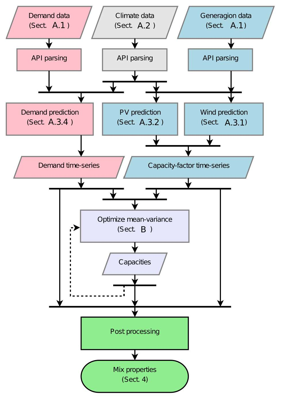
2. Methodology and Software Design

The purpose of this section is to outline the design of e4clim. To show its full potential, this description remains voluntarily abstract, while the next Section 3 gives the concrete implementation of the climate-aware mean-variance analysis.
Summarizing some of the methodology’s main objectives (Section 1), the e4clim software is a flexible tool allowing for the evaluation of energy mixes, taking into account the variability of the demand and production, from both mature and emerging technologies, on a broad range of time scales. An energy mix is defined here as a set of georeferenced capacities (e.g., at the scale of bidding zones, administrative regions or states) per energy source and may be prescribed, e.g., taking the actual mix of a given area, or optimized, e.g., with the mean-variance analysis detailed in the next Section 3. We are interested in properties of the energy mixes such as the mean penetration, the variance, the frequency of occurrence of critical situations, costs, GHG emissions, etc. These properties may provide the objectives of an optimization problem or may be computed ex post. They are computed from georeferenced energy data, such as demand and capacity factors per source and electrical region. The software’s stand-alone design is such that the whole chain of operations is covered, from downloading the data from its original sources to representing the results.
In e4clim, energy time series may be taken from observations directly. However, in order to consider new technologies and to resolve the impact of low-frequency variability on the production, it is also possible to estimate energy data by applying statistical models to climate time series, e.g., of temperature, wind speed or irradiance. To summarize, an e4clim project is divided in three phases:
  • Computing georeferenced energy time series from historic or climate data,
  • Distributing capacities spatially and technologically,
  • Post-processing and analyzing the resulting mixes.
A project thus takes as input energy, climate and geographic data to output mixes of georeferenced VRE capacities and properties that may be derived from this data.
Energy mixes are based on several components, i.e., loads or sources (wind, PV, etc.) for which georeferenced time series of relevant variables (demand, capacity factors, etc.) must be estimated or parsed, for a given area (e.g., a country or a macro region). The algorithms used to compute these variables are composed of statistical models made of sequences of blocks, and of data sources required by the models (see Appendix A for a description of the models and data sources used in the application of Section 4). Statistical models and data sources are, however, independent from each other and connected through a standard interface. New algorithms may thus be composed by assembling different sources and models. In particular, it is possible to either use energy observations provided by utilities directly, or to rely on statistical learning to fit existing or new demand/production models to observations and make predictions over a longer/future period from climate data.
These time series are then used in the optimization step and for the mix analysis together with installed capacities. In the future, controllable solutions (production, storage) could be dispatched in this post-processing stage to compute economic/carbon costs associated with the satisfaction of the mismatch between the demand and the VRE production.

3. A Concrete Implementation for Mean-Variance Analyses
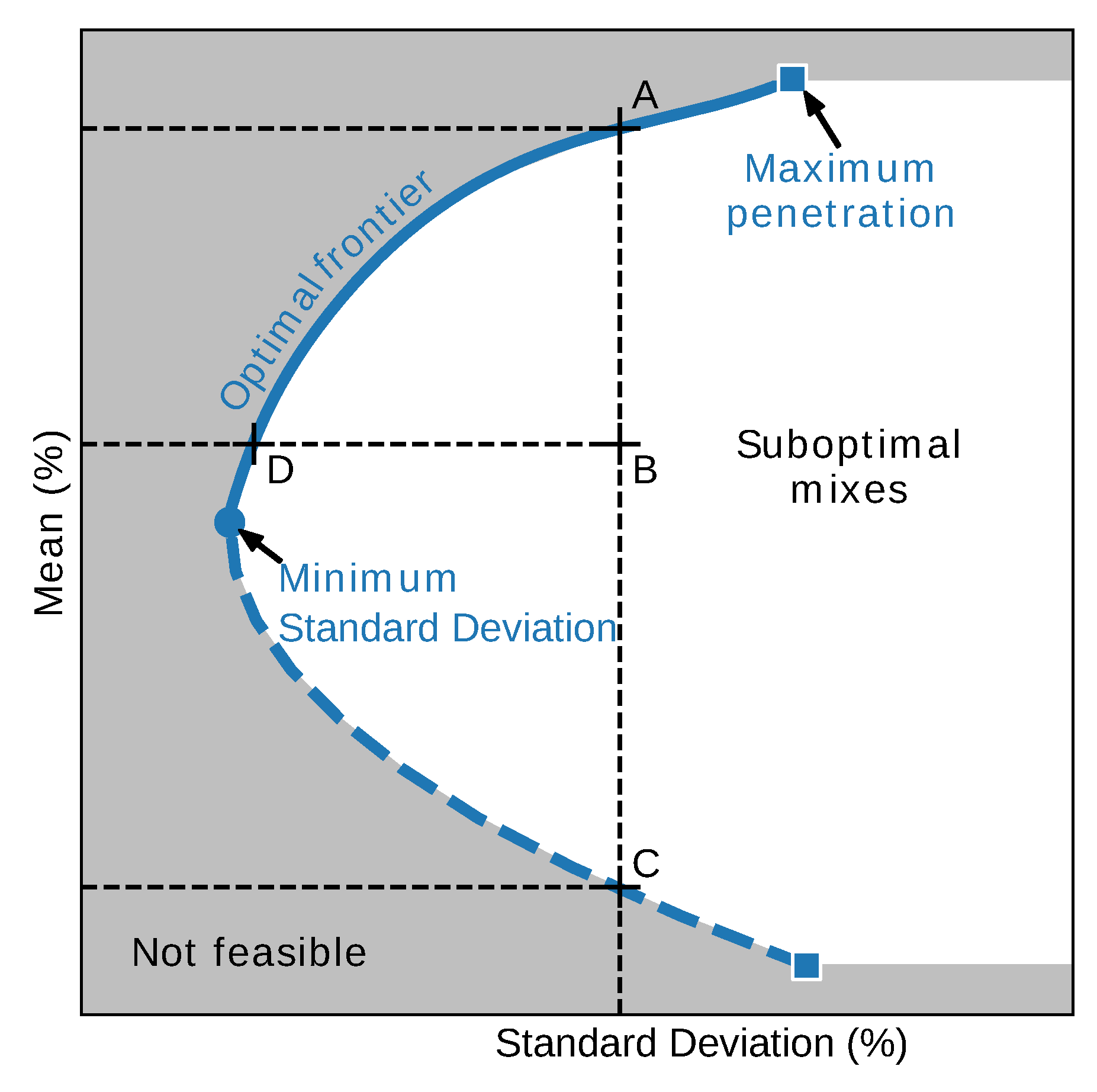
We now describe the implementation in e4clim of the mean-variance analysis applied in the next Section 4. The corresponding flow chart is given in Figure 1. Energy, climate and geographic data are used to compute optimal mixes and their properties. We base the computation of optimal mixes on a mean-variance analysis both to consider different optimal mixes and to limit the complexity of the program to the optimization of the VRE capacities. We assume that all installed VRE capacities are fully operational, that all the VRE production is injected to a copper plate network in which maximum transfer capacities are sufficiently high to prevent congestion (no constraints on the transmission) and that the mismatch between the actual demand and the VRE production is satisfied by conventional plants or other means. Assumptions about these plants are not needed at this stage since costs evaluation and more realistic constraints are left for future works.
We now proceed backward from the end of Figure 1 to describe this program.

3.1. Mix Analysis

The “post-processing” (quoted expressions refer to blocks in Figure 1) step translates capacities into mix properties such as the PV fraction and shortage and saturation occurrence frequencies (see plots for Italy in Section 4). This step may be further developed to compute economic costs and GHG emissions associated with a mix, etc.

3.2. Mix Optimization

In e4clim, a mix is either prescribed, or obtained as the solution of an optimization problem. In order to isolate the optimization of the VRE capacities from other energy systems, we use a “mean-variance” analysis of the VRE production with respect to the demand. The latter is based on two measures: the mean penetration,
μ ( w ) : = E k = ( i , j ) I × J w k η k ( · ) i I D i ( · ) = k = ( i , j ) I × J w k E η k ( · ) i I D i ( · ) ,
and what we refer to as the global version of the total variance,
σ global 2 ( w ) : = V k = ( i , j ) I × J w k η k ( · ) i I D i ( · ) .
(Here, k = ( i , j ) is the multi-index composed of an index i in the set I of zones, or electricity regions, and a technological index j in the set J of energy sources. The bold-faced symbol w denotes the vector with components w k giving the installed capacities for each region and technology. The η k ( t ) are the corresponding time-dependent zonal capacity factors and the D i ( t ) are the zonal demands (Appendix A.3). We refer to the ratios η k ( t ) / i I D i ( t ) as the normalized capacity factors. The symbol Σ denotes the sum over the index in subscript. The symbols E and V respectively denote the expectation and the variance of the random variable within brackets. In the following numerical applications, these statistics are replaced by sample estimates from the climate record [82].)
In other words, the mean penetration, μ ( w ) , and the global variance, σ global 2 ( w ) , are respectively given by the mean and the variance of the ratio between the total PV and wind production over the total demand. The variance serves as a proxy for flexibility services: minimizing the variance corresponds to maximizing the diversification of the renewable configuration, which in turn lowers the variability of renewable energy penetration and improves the flexibility of the system and its resistance to shocks. In particular, a lower variance in the renewable energy mix is less demanding in services from conventional production (for which start up and shutting down services have a cost) or demand management (see below).
Two alternate versions of the total variance are also considered. The technology variance,
σ technology 2 ( w ) : = i I V j J w ( i , j ) η ( i , j ) ( · ) i I D i ( · ) ,
is defined as the sum over zones of the variance of the total PV and wind production per zone over the total demand. The base variance,
σ base 2 ( w ) : = k = ( i , j ) I × J V w k η k i I D i ( · ) .
is defined as the sum over zones and technologies of the variance of the production per zone and technology over the demand (we discuss the implications of these alternative definitions regarding the optimization problem below) (Formally, these two measures do not correspond to a variance but to sums of variances).
Taking the mean penetration, μ , and a version of the total variance, σ 2 , as two objectives, the mean-variance analysis translates into an optimization problem distributing PV and wind capacities:
         min w   σ global|technology|base 2 ( w )
max w   μ ( w )
subject to   k w k = w total
       w k 0     k ,
Here, the Equations (5a) and (5b) are the two objective functions. Equations (5c) and (5d) are respectively an equality constraint fixing the total VRE capacity to some value, w total , and an inequality constraint preventing VRE capacities to be negative. In Section 4, we analyze results with and without the total VRE capacity constraint (5c).
Before to discuss the technical signification of this optimization problem, let us describe the mathematics. As a biobjective optimization problem [83], there exists a set of Pareto-optimal mixes, the optimal frontier. Each optimal mix may be represented in a mean-variance chart, as illustrated in Figure 2. A solution is said to be Pareto optimal if there exists no feasible solution with a better or equal value for each of the objective functions. The points under or to the right of the frontier are by definition suboptimal and will be discarded by a rational investor. The area above or to the left of the frontier cannot be reached. A detailed description of the mean-variance analysis procedure is given in Appendix B.
From a technical point of view, problem (5) is equivalent to minimizing the mean and the variance of the mismatch between the demand and the VRE production. Thus, assuming that this mismatch is satisfied by the conventional production (e.g., thermal and hydroelectric power plants), we expect that the mix minimizing economic costs from the conventional production and the mix minimizing GHG emissions are close to one of the mixes on the optimal frontier of (5). Before to discuss this heuristic further, let us mention that, although not a formal result, it allows one to limit the complexity of the optimization problem by reducing it to the optimization of VRE capacities, independently from conventional systems, thus making this methodology appropriate for sensitivity studies.
Quantifying the degree to which this heuristic is valid depends on the energy systems considered and is out of the scope of this study. However, let us remark the following. Overall, economic costs can be decomposed in: (i) fixed costs (e.g., capital expenditures, running costs); (ii) costs proportional to the megawatt-hours produced (e.g., operating expenses); and (iii) nonlinear costs (e.g., start up and shutting down costs during shortage or congestion situations). GHG emissions also include: (i) fixed life-cycle emissions associated with infrastructures; (ii) emissions due to fossil-fuel combustion in thermal power-plants at nominal power and proportional to the megawatt-hours produced; and (iii) nonlinear emissions, e.g., associated with generation regime changes. Maximizing the mean VRE penetration thus corresponds to minimizing costs or emissions proportional to the production needed to satisfy the mismatch between the demand and the VRE production. On the other hand, minimizing the variance accounts for part of the nonlinear costs and emissions resulting from satisfying the mismatch at each time step. Note, however, that costs are usually higher for shortage than for surplus situations, an asymmetry that is not reflected by the variance.
Finally, the three versions of the variance are based on aggregating the production and the demand, ignoring both network constraints and exchanges with other countries. By minimizing the global variance (2), weaker covariances between regions and technologies are leveraged. We refer to this case as the global strategy. Regarding the two other strategies considered, the technology variance (3) ignores covariances between different zones, while the base variance (4) ignores all covariances between different zones and technologies. Comparing mixes from these strategies thus allows us to assess the benefits from technological and geographical diversification.

3.3. Energy Models

We base the recommissioning study of Section 4 on historical data, so that resulting mixes are optimal for the historical period covered (1979–2012) (if the statistics are stationary and if the period covered is sufficiently long for sample means to converge, the mixes are also optimal for future periods). A proper estimation of the mean penetration and the variance is key to the mean-variance analysis. “Demand” and “capacity factor time series” are thus needed.
While computing the mean does not require data at a particular sampling frequency, the variance should be computed from long time series at a high sampling frequency to measure variability on a sufficiently wide range of time scales. Indeed, the variance of the renewable production, and, to some extent, of the demand, stems from climate variability and is distributed over a broad range of spatial and temporal scales [84]. VRE systems operating during several decades, they are impacted by year-to-year variability. On the other hand, several power markets operate with an hourly resolution (day-ahead) and several types of dispatchable power plants react on these time scales [22]. Moreover, Heide et al. [38] show that mismatch dynamics on intraday time scales have a large impact on optimal mixes. Here, we do not consider time scales smaller than an hour, that are essential when balancing the frequency using reserves [8].
In order to take time scales ranging from hours to decades into account and to be able to integrate additional capacities or new technologies for which no or little data is available, time series of the demands and capacity factors per zone are computed from climate data. On the other hand, energy estimates from climate data are prone to be biased compared to observations [73,74,85], so that they need to be adjusted statistically. To do so:
  • the “wind” production is “predicted” from wind data fed to a power curve at each grid point of the climate data (Appendix A.3.1), summed over each zone, and bias corrected against wind production observations (Appendix A.3.3),
  • the “PV” production is computed from surface irradiance and temperature data fed to an electric model (Appendix A.3.2), summed over each zone, and bias corrected against PV production observations (Appendix A.3.3),
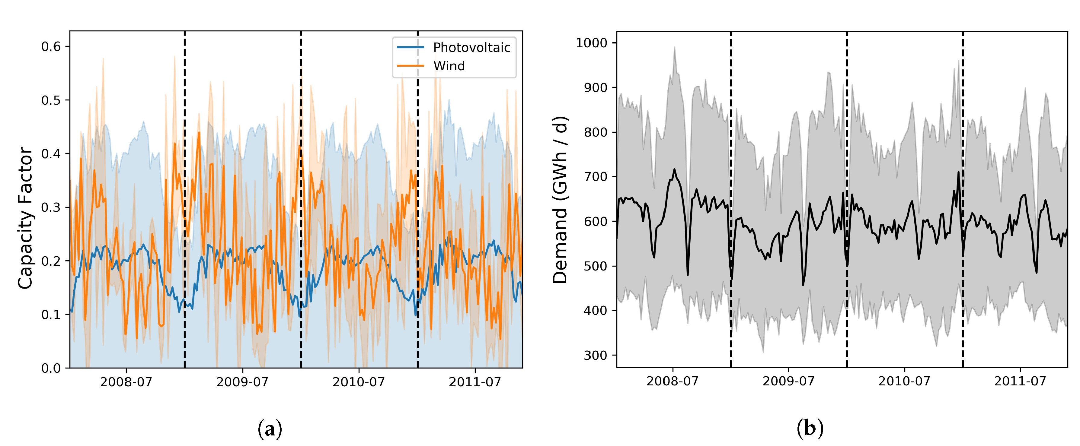
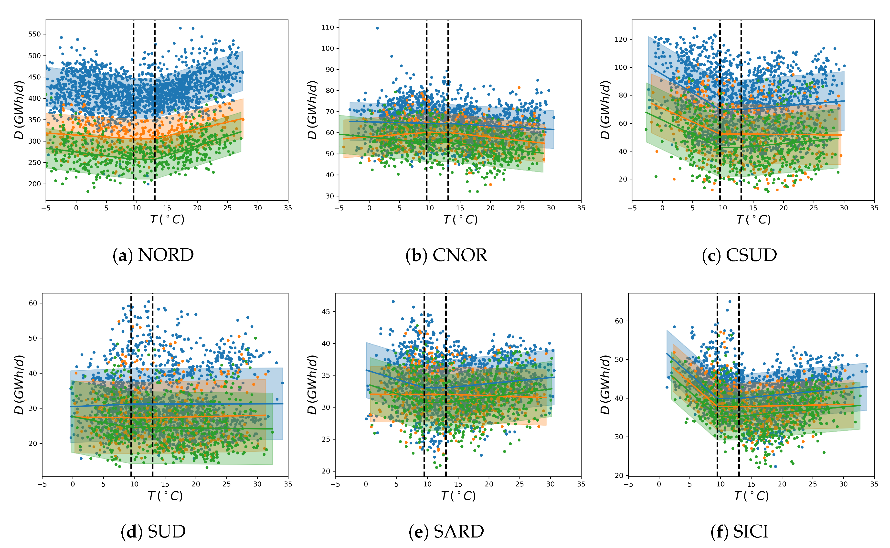
  • the “demand” is estimated via a linear Bayesian regression model taking as input warming and cooling degree days averaged over each zone and fitted to demand observations (Appendix A.3.4).
Although these models are key components of the concrete implementation of the software for the application of Section 4, we prefer to encourage the reader to learn more about them in Appendix A.3.
Importantly, when used with daily mean climate data, these models include a parametrization of intraday fluctuations. Results from the application are indeed derived from the daily mean climate data (Appendix A.2.1). We have made this choice to illustrate the possibility to use this software with daily mean climate data, more of such data being available than hourly climate data.

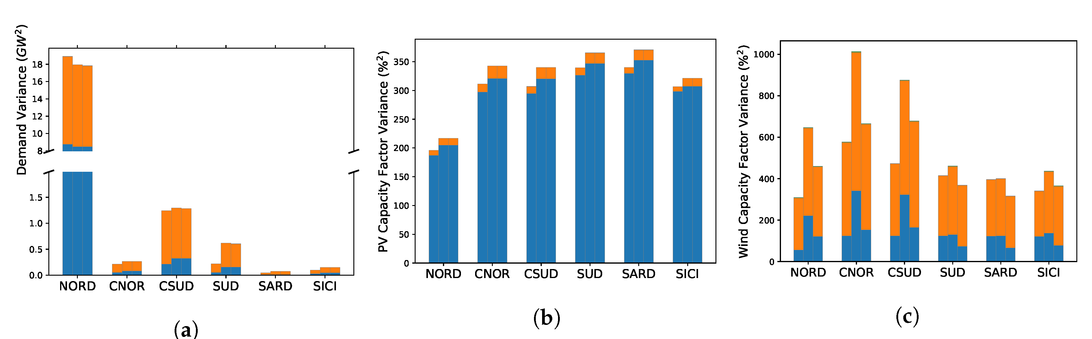
3.4. Energy, Climate and Geographic Data

The energy models rely on “demand”, “generation” and “climate data”. Application Programming Interfaces (APIs) are developed to download and format the required data (“API parsing”). Downstream, e4clim data management follows a standard format allowing one to use different data sources for the same function. In particular, several climate data sources may be used to assess biases stemming from the latter. The data sources used for the application of the next Section 4 are described in Appendix A.1 and Appendix A.2. We use hourly electricity-demand data per zone from the market operator, GME; yearly mean capacity-factors per zone from the TSO; daily mean regional climate data from CORDEX; and hourly global climate data from MERRA-2 (only for the intraday parametrization and the evaluation). Finally, the regional boundaries used to map grid points from the climate data to regions are obtained from GISCO (https://ec.europa.eu/eurostat/web/gisco).

4. Application: Italian PV-Wind Optimal Recommissioning

We now present the application to the Italian PV-wind mix illustrating the potential of the methodology and the software. We focus on Italy and its six bidding zones, or electrical regions, as shown in Figure 3a. Italy offers an interesting case study of a market with a high VRE penetration as it has reached its quota of 17% renewables in final energy consumption in 2014, therefore implementing the 2009 Climate Package six years ahead of the 2020 horizon [86]. Figure 3b represents the geographical distribution of the installed PV-wind capacities. The PV (wind) installed capacity is 18 . 9 GW ( 9 . 2 GW). The share of the renewable energy production in the electricity demand over the six zones was 19.4% in 2015.

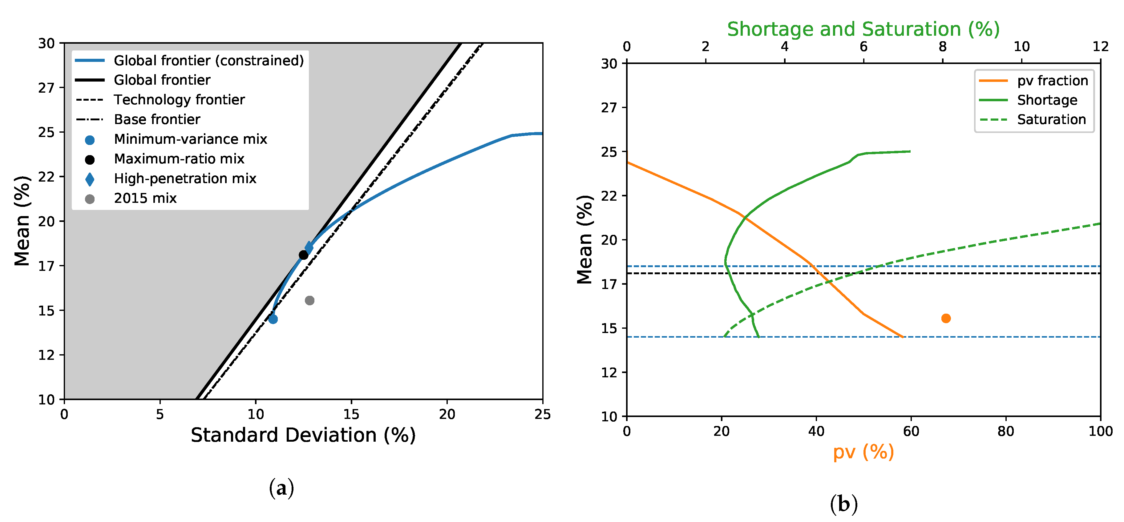
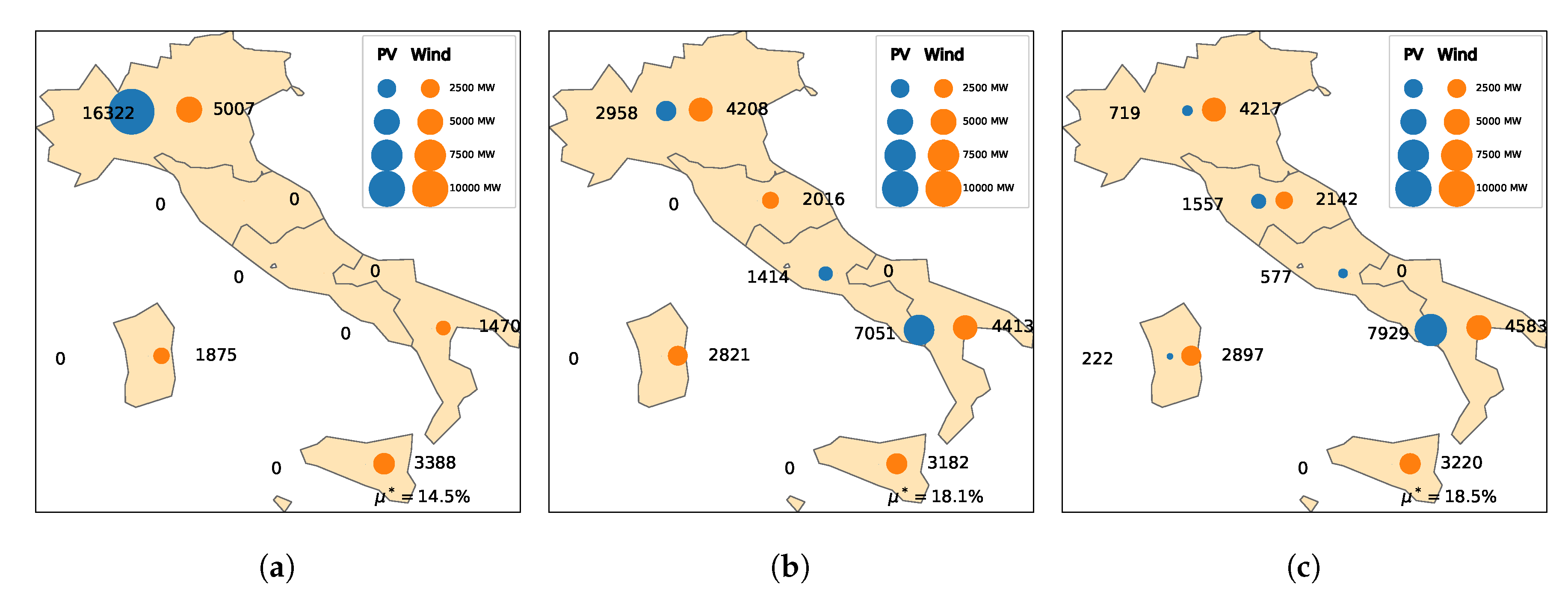
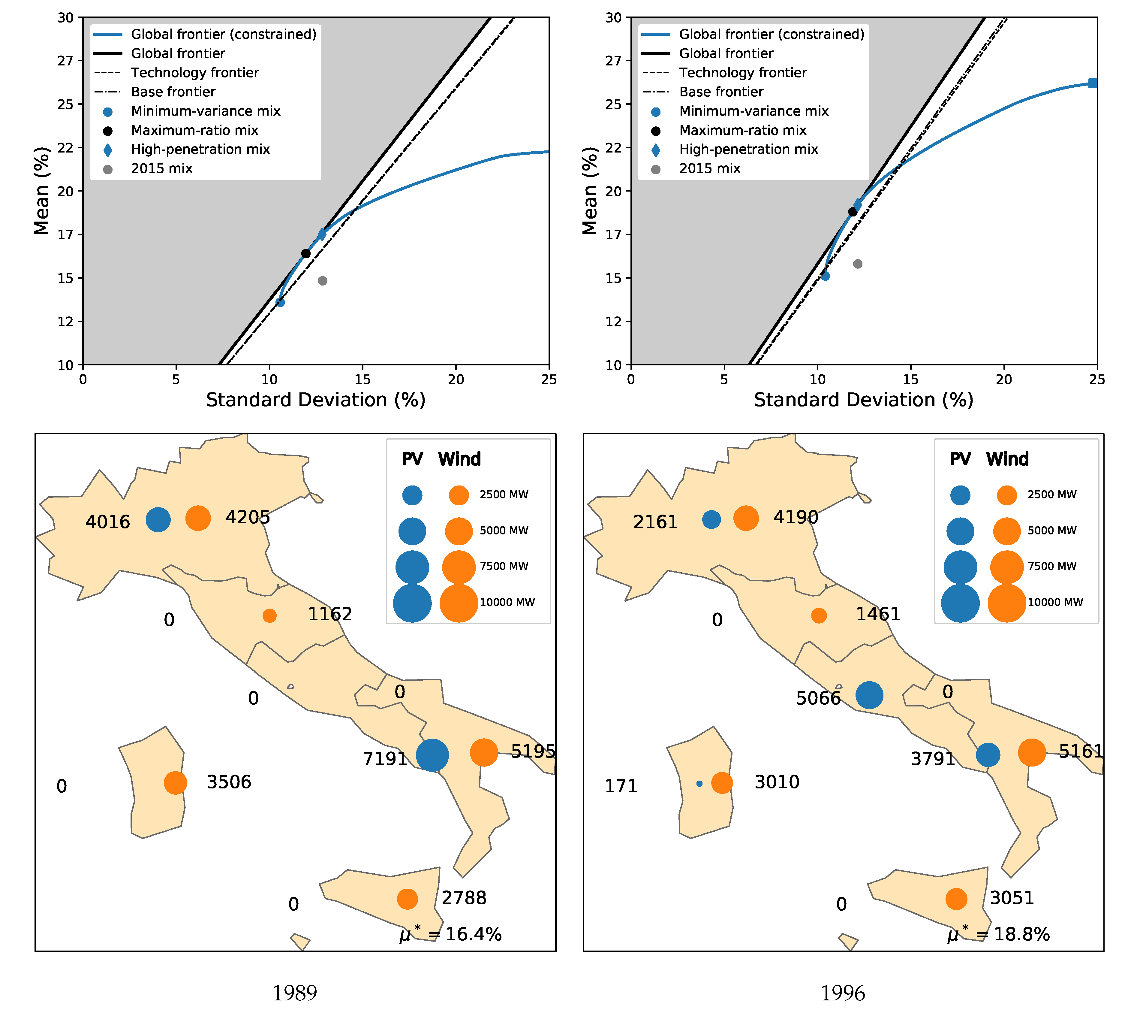
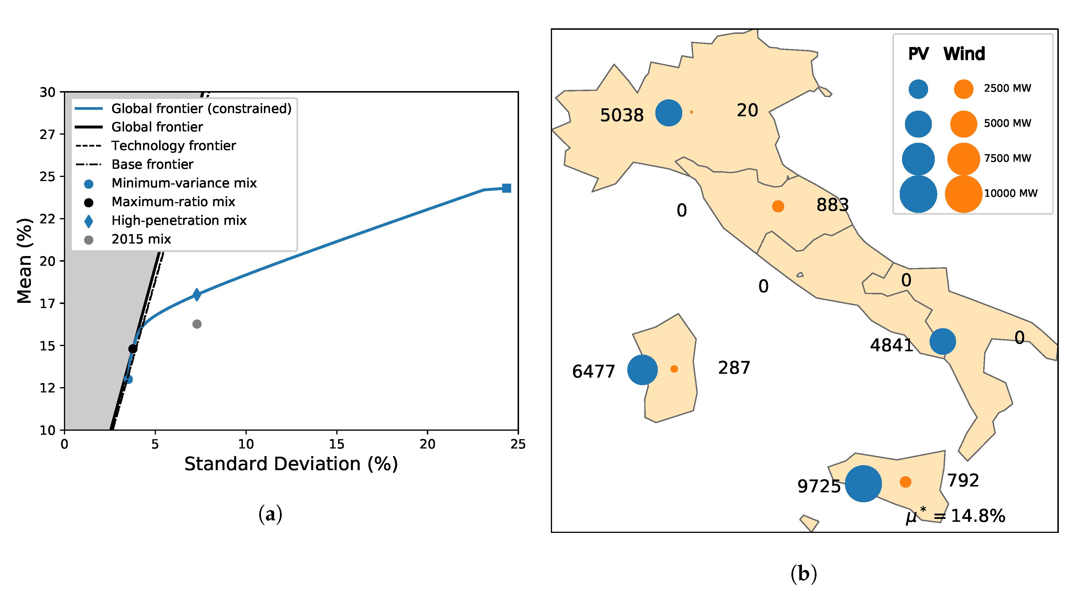
4.1. General Results

We represent the optimal frontiers obtained from the CORDEX data [87] with the intraday parametrizations over the 1989–2012 period (Appendix A) in Figure 4a. Four different frontiers are represented. Each point of a frontier represents an optimal distribution of the PV and wind capacities. Representing frontiers rather than single optimal mixes leaves more space for arbitrages between mixes with higher shares of VREs and mixes requiring less flexibility (low variance). The latter could in turn be guided by associated costs, GHG emissions, expert knowledge, values, etc.
Two variants are represented in Figure 4a: one in which the total capacity is constrained (plain blue curve), and one without such constraint (plain black curve). We can see that the optimal frontier without the total-capacity constraint (thick black line) is a straight line passing through the origin. Its slope, the mean-standard deviation ratio, is of 1.44 . In other words, letting the square root of the global variance increase by 1.00 % results in an increase of the mean penetration by 1.44 % , at best. Thus, this ratio gives a simple diagnostic to compare different unconstrained frontiers.
On the other hand, the frontier with the constraint allows us to consider the optimal recommissioning of the VRE capacities for the total capacity of 28.1 GW installed in 2015 in Italy. In this case, the frontier bends away from the unconstrained one to the right, as the additional constraint renders the minimization of the variance more difficult. The point in Figure 4a at which both curves intersect represents the mix for which the total-capacity constraint is inactive (satisfied without the need to force it). It is thus the optimal mix satisfying the total-capacity constraint that has the maximum mean-standard deviation ratio, the maximum-ratio mix. If no preference is put on maximizing the mean penetration or on minimizing the variance, this optimal mix is the most attractive mix satisfying the total-capacity constraint.
For a recommissioning, one may, however, be interested in allowing for the deterioration of the mean-standard deviation ratio in order to either decrease the variance or increase the mean penetration. The blue dot in Figure 4a corresponds to the optimal mix minimizing the variance while satisfying the total-capacity constraint, the minimum-variance mix. For comparison with the actual mix, the blue diamond in Figure 4a represents the optimal mix satisfying the same level of variance as the actual mix (gray dot, see Section 4.2) while maximizing the penetration rate, the high-penetration mix (The high-penetration mix corresponds to the EqRisk mix considered by Santos-Alamillos et al. [54]).
Benefits from interconnections between zones and synergies between technologies can be assessed by comparing the frontiers obtained for the global, technology and base strategies. The technology and base frontiers without the total-capacity constraints (respectively the dashed and point-dashed thin black lines in Figure 4a) roughly coincide. Therefore, taking local correlations between the normalized PV capacity factors and the normalized wind capacity factors into account do not significantly reduce the variance. The technological complementarity is weak. However, with a mean-standard deviation ratio of 1.37 and 1.38 , respectively, these frontiers lie to the right of the global frontier (plain black line). Thus, for a given level of mean penetration, taking correlations between zones into account allows one to reduce the standard deviation by about 4.9 % . A significant level of smoothing is achieved through geographical diversification.
Properties of the optimal mixes along a frontier may then be derived. To illustrate this, the fraction of PV capacity in mixes (orange) and the shortage (plain green) and saturation (dashed green) frequencies are represented in Figure 4b, for the global strategy with the total-capacity constraint. Shortage and saturation situations are examples of critical situations expected to become more problematic with increasing shares of VREs [3]. Here, it is assumed that conventional generation units are able to meet up to 80 % of the modeled-demand maximum. Shortage then occurs if the PV and wind generation is not able to meet the rest of the demand. The second critical situation corresponds to network saturation, when PV and wind production exceeds technical limits of renewable energy fraction in the mix. In this study, saturation is defined to occur if more than 40 % of the demand has to be met by PV and wind sources.
Because wind capacity factors are higher than PV ones, the PV ratio in Figure 4b is a decreasing function of the mean penetration. The shortage and the saturation curves (in green) have distinct global minima due to the increase of the probability of occurrence of extremes with the variance. The vertical lines in Figure 4b represent the level of mean penetration for the minimum-variance, maximum-ratio and high-penetration mixes. The minimum-variance, the maximum-ratio and the high-penetration mixes respectively include 58 % , 41 % and 39 % of PV capacity in the mix. Saturation situations occur less often for the minimum-variance mix, while the maximum mean-standard deviation ratio and the high-penetration mixes are close to the shortage-occurrence minimum. Together with costs and GHG emissions (not implemented yet) these properties and the analysis of their behavior along a frontier may guide the choice of mixes and help evaluate their sensitivity to changes in the target mean penetration or variance.
Finally, the geographic distribution PV-wind capacities of different mixes may be represented, as in Figure 5, to compare them. Significant differences exist between these mixes, showing that the optimal distribution is relatively sensitive to the objectives.
To summarize, optimal mixes and their properties strongly depend on the level of variance that is tolerated. As a consequence, capacities are not necessarily distributed where they would be expected based on the resource mean potential only.

4.2. Comparison with the 2015 Italian Mix

The 2015 (actual) Italian mix (Figure 3b), is composed of 67 % PV and 33 % wind energy capacity. For historic and economic reasons, the largest fraction of installed PV capacity is in the North of Italy, whereas most of wind capacity is located in the South.
To compare the optimal mixes discussed so far with the actual 2015 Italian mix, it is possible to provide the latter to the e4clim post-processing step directly (Figure 1). This mix is represented by the gray point in Figure 4a. It lies to the right of the optimal frontiers. The actual Italian mix thus appears to be suboptimal. For the global problem, this mix reaches a level of mean penetration comparable to that of the minimum-variance mix (larger by 1.0 % ), but its mean-standard deviation ratio is larger by 1.9 % and its PV ratio (orange point in Figure 4b) larger by 9.2 % .
By comparing the actual capacity distribution in Figure 3b with one of the optimal mixes in Figure 5, we can see that the actual mix has less wind capacity in the northern regions and more PV capacity everywhere.

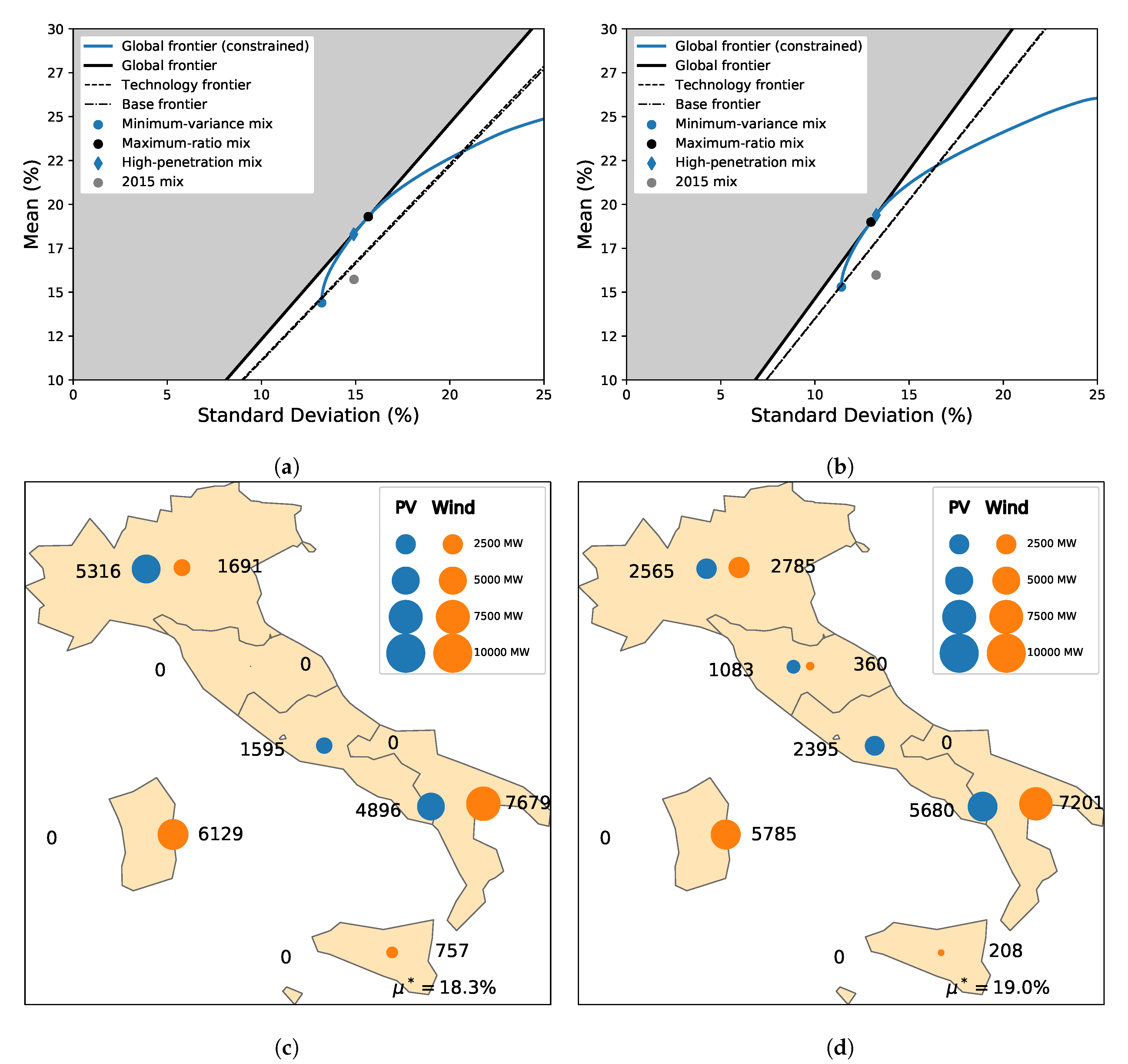
4.3. Choice of the Climate Data and Climate Variability

By estimating the energy production and demand from climate data with e4clim, we can discuss the impact of climate variability on mixes, change the distribution of capacities within a zone (which affects the zonal capacity factors) and study the impact of the introduction of new technologies. On the other hand, climate-data biases may also impact the quality of the results [73,85], thus calling for multi-model approaches. Both points are now discussed.

4.3.1. Dependence on the Climate Data

The robustness of the mean-variance analysis presented in Section 3 depends on the quality of the energy estimates from the climate data. The latter is in turn impacted by climate-model biases. With the e4clim software, it is possible to use different climate-data sources to test the sensitivity of the results to biases stemming from the climate data.
To illustrate this point, we compare the results of Section 4 obtained with the daily CORDEX data with the intraday parametrizations (Appendix A.3) with results obtained from hourly simulations from the MERRA-2 reanalysis (Appendix A.2.2), over the same period (1989–2012). With this dataset, no intraday parametrizations are needed. Divergence in the results may thus stem both from differences in the climate data and from these parametrizations. In summary, the MERRA-2 reanalysis presents the advantage to be hourly sampled and to cover a longer period (1980–present), while the CORDEX data presents the potential for using projections for the 21st century. Last, both the 10 m and the 50 m winds are provided in the MERRA-2 dataset. Comparing results using either winds is interesting because 10 m winds are expected to be more impacted by surface friction and because 50 m winds are closer to the hub height (101 m).
Figure 6 shows the approximated optimal frontiers (top) and the corresponding capacities for the mix maximizing the mean-standard deviation ratio of the global strategy (bottom) obtained by applying the hourly demand and capacity-factor models to the MERRA-2 data using 10 m winds (left) and 50 m winds (right). Overall, the qualitative picture of the frontiers remains unchanged (cf. Figure 4a), but important quantitative differences exist. First, the mean-standard deviation ratio for the MERRA-2 data with 50 m winds, with a value of 1.46, is close to that for the CORDEX data (1.44), but is larger for the MERRA-2 data with 10m-winds by about 15 % . This difference in the ratios is in fact larger that that of 4.9 % found between the global and the technology strategies with the CORDEX data. Differences between the capacity distributions also exist between all three cases, but perhaps less so between the MERRA-2 with 50 m winds maximum-ratio mix and the CORDEX high-penetration mix. This shows that differences between capacity distributions may exist even if the mean-standard deviation ratios are similar.
Differences between the mean-variance analyses using the CORDEX data and the MERRA-2 data may stem from discrepancies in the means of the estimated demand and capacity factors. However, the latter are practically indistinguishable (not shown here), due to the regressions against observations (see Appendix A.3). Differences may instead be due to the variances and covariances of the estimates. We compare in Figure 7, the variance of the electricity demand (left), PV capacity factor (middle) and wind capacity factor (right) explained by periods greater than a year (green), less than or equal to a year (orange) and greater than a day, and less than or equal to a day and greater than an hour (blue). These values are estimated (i) from the models applied to the daily CORDEX data (left bars); (ii) from the models applied to the MERRA-2 data with 10 m wind (middle bars) and 50 m wind (right bars) (the variance explained by each frequency band is calculated from the variance of the respectively low-pass, band-pass and high-pass filtered time series using rolling averages as filters).
In all cases, interannual variability is very week, although non-vanishing for the wind capacity factors. Differences between the MERRA-2 10 m and 50 m wind results only impact the wind capacity-factor estimates, although differences exist in the demand due to the stochastic nature of the Bayesian model. The electricity demand and PV capacity-factor estimates are relatively close between the CORDEX and the MERRA-2 data, although the CORDEX intraday variance of the PV capacity factors tends to be underestimated compared to the MERRA-2 estimates. This could be explained by the fact that the intraday parameterization used to estimate the hourly PV capacity factors from the daily CORDEX data neglects intraday variations of the clearness index (see Appendix A.3.2). Most differences between the CORDEX and the MERRA-2 estimates are for the wind capacity factors. Indeed, the intraday variance computed from the MERRA-2 10 m winds is larger than for the other two cases and the seasonal variance computed from the MERRA-2 10 m and 50 m winds is also larger that for the CORDEX winds. These differences are likely to be responsible for the changes in the mean-variance analysis results.
This shows that the sensitivity of the mean-variance results to the climate data can be large. Care should thus be taken to test this sensitivity, e.g., via multi-model approaches.

4.3.2. Interannual to Decadal Variability

To assess the impact of interannual climate variability (as found in the CORDEX data) on energy mixes, we repeat the mean-variance analysis successively using data blocks of one year, from 1989 to 2012, rather than using the full 1989–2012 block. In other words, each of the 23 optimal frontiers are optimized for the climatic conditions of a given year and low-frequency climate variability results in different optimal mixes for each year. The mean-standard deviation ratio for the unconstrained global frontier can be used as a synthetic observable of these changes. It is found to average to 1.43 and to range from 1.37 to 1.58 . Thus, even though the average of the yearly mean-standard deviation ratio is close to the one of 1.44 obtained using the full record in Section 4.1, interannual climate variability in the CORDEX data is responsible for year-to-year variations of the mean-standard deviation ratio of up to 11 % . As an example, we represent in Figure 8 the geographical and technological distributions of the mixes for the year 1989, with a particularly low mean-standard deviation ratio of 1.37 , and for the year 1996, with a particularly high mean-standard deviation ratio of 1.58 .
These preliminary results show (i) that e4clim is able to resolve some interannual variability associated with climate fluctuations and (ii) the importance of assessing VRE mixes over several years of data to take into account the impact of interannual variability on mixes. (We leave the validation of this variability against observations for future work. However, the representation of interannual climate variability in the CORDEX and MERRA-2 datasets has been studied in previous works. See Ruti et al. [87] and Long et al. [88].)

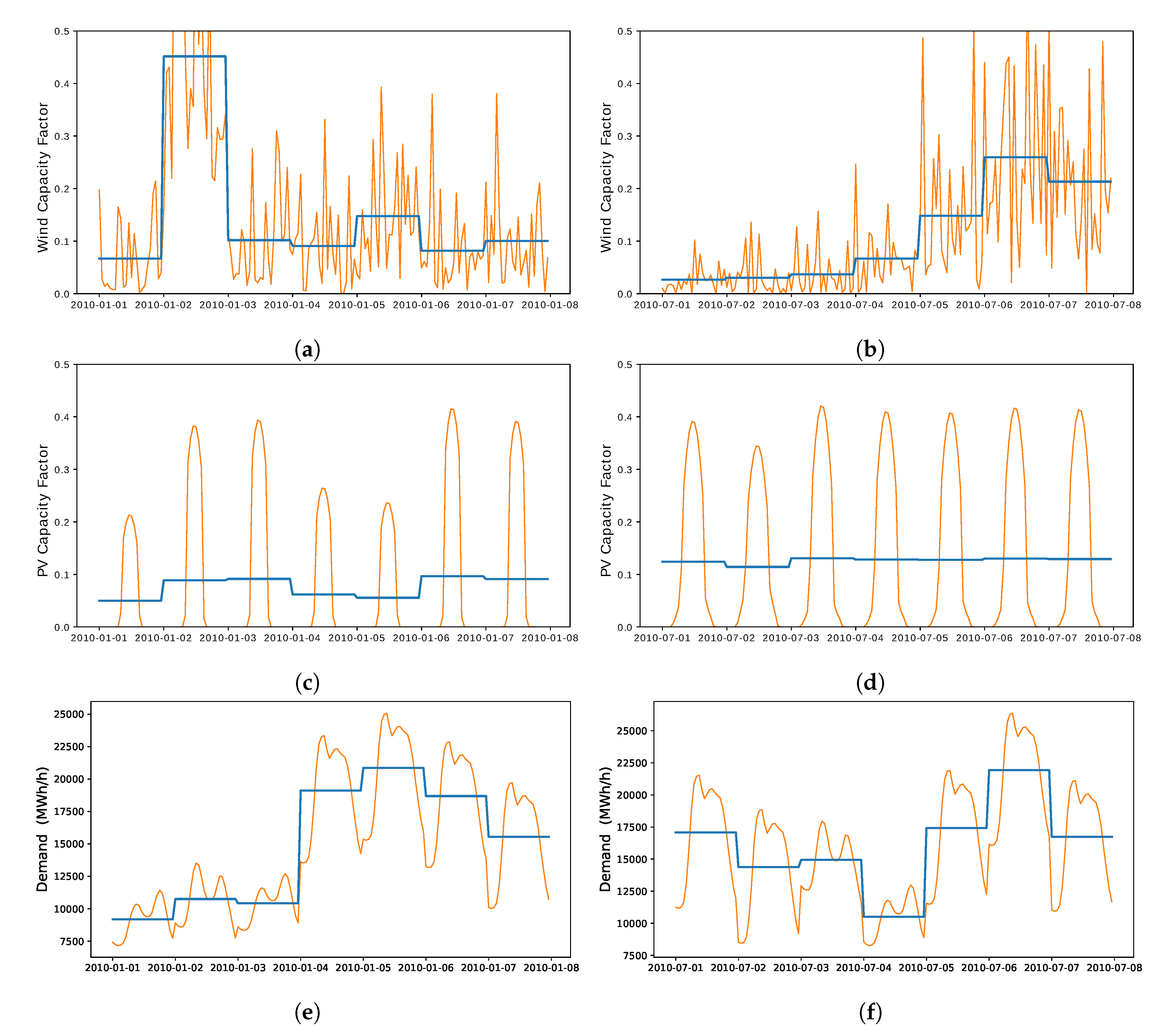
4.3.3. Intraday Variability

A large fraction of the PV, demand and wind variance is contained in the intraday range. Yet, climate data is not always available at an hourly sampling. This is for instance the case of the CORDEX data used here, for which intraday parametrizations are added to the energy models (Appendix A.3). To test the impact of ignoring such fluctuations on the optimal mixes, we represent in Figure 9 optimal frontiers (left) and the PV-wind distribution of the maximum-ratio mix (right) obtained directly from the daily CORDEX data without intraday parametrizations. It is clear that the standard deviation is underestimated by a factor two or more compared to the one obtained using hourly data (c.f. Figure 4 and Figure 5). This can be understood from the fact that, while the mean capacity factors remain unchanged, the variance in the modeled daily PV and wind capacity factors is dramatically underestimated (see Appendix A.3.3). Because the PV production is more variable during the day than the wind production, ignoring intraday fluctuations results in distributing more PV capacities. Here, we do not discuss the impact of variability on time scales shorter that an hour. The latter are, however, important when assessing the stability of the network.

5. Conclusions

This work is aimed at developing a modeling tool dedicated to the assessment and elaboration of optimal energy mixes taking into account flexibility needs associated with higher shares of VRE. It relies on mean-variance analysis to allow decision makers to arbiter between different strategies and mixes and offers the potential for low-frequency climate variability to be resolved and for new technologies to be integrated. This methodology is implemented as an extensible open-source Python software, e4clim. Its potential is demonstrated with an application to a recommissioning of the 2015 Italian PV-wind mix. However, this application is but one example of possible implementations within e4clim.
The software’s flow is divided in three steps: (i) energy time series are first estimated from climate data and fitted to observations; (ii) a VRE mix is then prescribed or optimized by, e.g., mean-variance analysis; (iii) the mix properties are finally analysed. The first step relies on climate data to take production and demand variability on a broad range of time scales into account and to allow for the integration of new technologies for which no or little observations are available. The current version of e4clim is also adapted to consider optimal strategies in a warming climate using 21st century regional projections provided by the CORDEX program (not shown here). We recommend using climate data from multiple independent sources to estimate errors stemming from these sources.
Different optimal scenarios are derived in the second step, ranging from maximizing the total renewable energy penetration to minimizing the variance, and so, flexibility requirements to meet the demand. Different strategies can quickly be tested, allowing one, for instance, to evaluate benefits from leveraging correlations between zones.
In addition to the mean and the standard deviation of the VRE penetration, we have illustrated the value of the ratio of these two metrics, the mean-standard deviation ratio, to compare different strategies. First, this ratio defines optimal frontiers for the unconstrained problems. Second, it provides a simple diagnostic to assess the extent to which leveraging weaker correlations between regions allows for the reduction of the variability of the aggregate production with respect to the demand. However, similar mean-standard deviation values for different cases do not preclude significant differences between the corresponding capacity distributions.
As opposed to cost-minimizing problems for full mixes, the mean-variance analysis allows us to focus on VRE capacities alone, thus limiting the complexity of the algorithm and making it a fast and flexible tool for sensitivity analyses. This leaves the estimation of associated economic costs and GHG emissions to the third (post-processing) step. For that purpose, the conventional production would have to be modeled with reserve, network and dispatch constraints. In addition, the application of this model to the Euro-Mediterranean region is a priority.

6. Known Limitations of the Software and Methodology

In order to facilitate further improvements and applications of the model, let us finish by mentioning some of the limitations of its current implementation (Section 3).
First, the domain of application of the software could be extended in several directions. For instance, it could include more renewable energy sources than PV and wind alone. To better evaluate the benefits from spatial and technological diversification, present or future network constraints could be added, for instance relying on a DC power-flow approximation with net transfer capacities (see e.g., Rodríguez et al. [39]). Flexibility services such as storage, demand management and imports/exports could also be added. Depending on the area considered, modeling such systems may be necessary to compute costs associated with energy mixes. An important question is whether these systems have to be part of the VRE-capacity optimization problem or whether they can be kept separate to limit the complexity of the model. Interfaces to other data sources may also be added to consider other areas than Italy.
Second, as discussed in Appendix A.3.3, the robustness of solutions to the mean-variance optimization problem depends on the accuracy of the inputs to this problem, namely, the vector of mean capacity factors and the covariance matrix entering the definition of the mean penetration (1) and of the variance (2). The latter being estimated from the climate data, they depend on the quality of the latter at regional scale. When observations of the yearly mean of the production and of the demand per zone are available, supervised learning can be used to correct for biases, as in this study. We have, however, directly corrected the capacity factors. Due to the nonlinear relationship between wind speeds and wind power, keeping expressing the loss function for the training in terms of capacity factors but correcting the wind speeds before to apply the power curve, as in Staffell and Pfenninger [73], could be more appropriate for climate change studies.
To further assess the accuracy of the estimates of the covariance matrix against observations, hourly observations per zone and technology are required. Such data is difficult to acquire. In the case of Italy, for instance, hourly data is provided by Terna and also available on the ENTSO-E Transparency Platform. However, the latter is not consolidated and the yearly means were not found to be consistent with yearly mean data provided by Terna separately.
A large source of error also stems from the assumption that VRE capacities are uniformly distributed within a zone and that the production is computed for an arbitrary technology. This ignores the fact that the most favorable sites within a zone may have been selected to install existing capacities. While the bias correction used here removes discrepancies in the zonal-mean capacity factors and demand, it does not correct for errors in the variance, nor does it take into account the fact that new VRE installations may not yield capacity factors as high as for existing installations, unless technologies improve.
Third, we have chosen the variance as a proxy for costs arising from the variability of the renewable production. This metric is symmetric, in the sense that negative and positive deviations from the variance are given the same weight. Yet, it is known that shortages in the production tend to cost more than excesses. The extent to which the mean and the variance are, together, good proxies for economic or GHG costs should be addressed. Other metrics such as the skewness could be considered and links to the micreconomic theory of energy markets made.

Author Contributions

Conceptualization, A.T., M.S., P.D., J.B., S.C., A.C. and P.T.; Data curation, S.C. and A.C.; Formal analysis, A.T., M.S. and P.D.; Funding acquisition, P.D. and P.T.; Investigation, A.T., M.S., P.D. and P.T.; Methodology, A.T., M.S., P.D., J.B., S.C., A.C., C.D. and D.T.; Project administration, P.D. and P.T.; Software, A.T., C.D. and D.T.; Supervision, P.D. and P.T.; Validation, P.D. and P.T.; Writing—original draft, A.T. and M.S.; Writing—review & editing, A.T.

Funding

This work was conducted in the framework of the TREND-X research program on energy transition at Ecole Polytechnique, which benefited from the support of the Ecole polytechnique fund raising—TREND-X Initiative. This research was also supported by the ANR project FOREWER (ANR-14-414 CE05-0028) and the HyMeX project (HYdrological cycle in The Mediterranean EXperiment) through the working group Renewable Energy, funded by INSU-MISTRALS program.

Acknowledgments

AT is grateful to Mathilde Mougeot and Jérôme Collet for insightful discussions on modeling the electricity demand. The authors would like to thank the reviewers for their careful reviews and suggestions which helped improve this article. The e4clim open-source software is available online under GPL license at https://doi.org/10.14768/20191105001.1 (accessed on 10th of November 2019). This page also links to the e4clim documentation, which includes all cases from this study.

Conflicts of Interest

The authors declare no conflict of interest. The founders had no role in the design of the study; in the collection, analyses, or interpretation of data; in the writing of the manuscript, or in the decision to publish the results.

Appendix A. Data and Model Description

An e4clim project relies on models to predict energy time series (demand and capacity factors) from climate data. These models depend on energy data to be fitted via regression or bias correction. The energy data, climate data and demand, PV and wind models are described here.

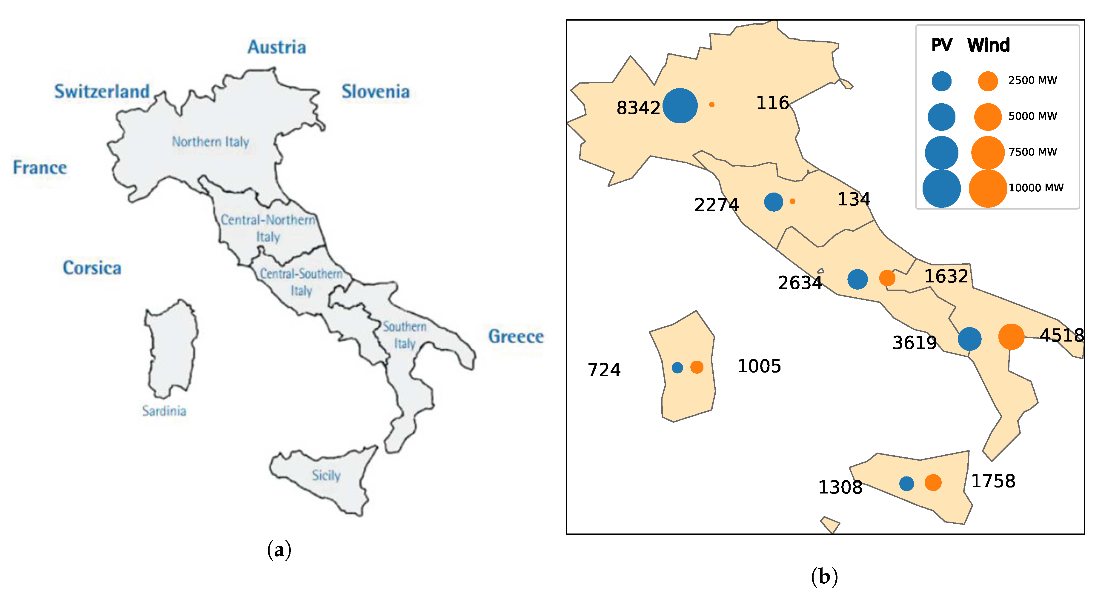
Appendix A.1. Energy Data: GME and Terna Databases

Time series of the hourly Italian zonal electricity demand and of the yearly zonal renewable capacity factors are used to train the demand and generation models. See the “demand” and “generation data” blocks at the top of Figure 1. These variables are extracted from three publicly available databases provided respectively by the market operator GME (Gestore del Mercato Elettrico: https://www.gse.it/dati-e-scenari/statistiche) and the Transmission System Operator (TSO) Terna (https://www.terna.it/en/electric-system/statistical-data-forecast/evolution-electricity-market). For this reason, we first briefly comment on the structure of the Italian electricity market and next describe the databases we use.
The Italian power market consists of 7 foreign virtual zones, 6 regional sub-markets, or bidding zones, and 5 poles of limited production. The 20 administrative regions composing the Italian territory are aggregated in the 6 bidding zones (Figure 3a): Northern Italy (NORD), Central-Northern Italy (CNOR), Central-Southern Italy (CSUD), Southern Italy (SUD), Sardinia (SARD) and Sicily (SICI). Each zone has its own generation mix determined by historical and geographic reasons and characterized by a given level of efficiency. For instance, the Northern regions have larger hydroelectric production due to the proximity to the Alps. Inter-zonal transmission capacities are not equally distributed either.
The Italian power exchange, which is managed by GME is composed of a spot market, a forward market and a platform for the physical delivery of contracts concluded on the financial derivatives segment of the Italian Stock Exchange. The spot market is composed of three submarkets: the day-ahead, the intraday and the ancillary services markets. We focus on the day-ahead submarket. The liquidity of the day-ahead market, calculated as the ratio of volumes traded on the day-ahead market to the total volumes (including bilateral contracts) of the Italian power system, has increased between 2010 to 2015, passing from 62.6% with 198 operators in 2010 to 67.8% with 259 operators in 2015. The peak liquidity has been reached in 2013 with a 71.6% liquidity and 214 operators (GME, 2017).
The GME database encompasses hourly bids and offers in the wholesale electricity market from 2005 to 2018; the offers are identified by supplier’s technology. The hourly electricity demand is appraised from this source. We select the demand data for the six aforementioned bidding zones only, accounting for about two third of the total demand including exports.
Terna’s statistical data contains information about the yearly electrical production and the associated installed capacity at the end of each year detailed by region and sources from the beginning of 2000 to the end of 2018. This corresponds to the longest dataset that we have found at the zonal scale. The time-mean capacity factors for PV and wind per zone are calculated from this source. At the beginning of the available period, the installation of VRE capacity shows a rapid increase. Moreover, PV capacity factors increase at a rate that cannot be explained by interannual climate variability until about 2010–2011 (not shown here). Since then, PV and wind capacity factors are relatively stable.
Note also that, although hourly wind and PV capacity factors may in principle be computed from the hourly generation and capacity provided by Terna over 2015–2018, the latter are not consolidated. Once averaged over each year, we have in fact found this data to be inconsistent with the corresponding consolidated yearly means provided by Terna separately. We thus do not have hourly data at our disposition to validate estimates at shorter time scales than a year against observations.
The demand and the PV and wind capacity factors per zone and averaged over the 2010–2018 period are presented in Table A1. Figure 3b summarizes the current installed capacity at the end of 2015.
Table A1. Yearly electrical demand (from GME) and yearly mean PV and wind capacity factors (from Terna) averaged over 2010–2018.
ZoneElectrical DemandCapacity Factor (%)
(TWh/y)(%)PVWind
NORD1215811.720.0
CNOR19.49.213.419.5
CSUD30.31413.918.9
SUD15.07.115.021.0
SARD10.85.114.418.5
SICI13.56.415.218.6

Appendix A.2. Climate Data

The mean-variance optimization problem (Appendix B) relies on electricity demand and PV and wind capacity-factor time series. Observed time series are only a few years long, too short to resolve low-frequency climate variability. The models described in Appendix A.3 are thus used to predict these energy time series from climate data. See the “climate data” block at the top of Figure 1. In this study, one particular CORDEX regional simulation is mainly used, that we refer to as the CORDEX data. This choice is motivated by the fact that, contrary to reanalysis products, CORDEX projections for the 21st century are also available, which could be used to apply the e4clim software to assess the impact of climate change on energy mixes in the future. Another climate dataset, the MERRA-2 reanalysis, is also used to (i) parametrize intraday wind-fluctuations not resolved by the CORDEX data (Appendix A.3.1) and (ii) test the dependence of the Italian-application results to the choice of the climate dataset in Section 4.3.1.

Appendix A.2.1. CORDEX Regional Simulations

The deployment of VREs being relatively recent (starting around 2008 in Italy), available time series of the observed VRE production are not sufficiently long to estimate statistics resolving low-frequency climate variability. To take it into account, the VRE production is instead computed using regional climate simulations covering a historical period (1989–2012).
We use the version 3.1.1 of the Weather Research and Forecasting Model (WRF). WRF is a limited area model, non-hydrostatic, with terrain following eta-coordinate mesoscale modeling system designed to serve both operational forecasting and atmospheric research needs [89]. The WRF simulation has been performed in the framework of HyMeX [90] and MED-CORDEX [87] programs with a 20 km horizontal resolution over the domain shown in Figure A1 between 1989 and 2012 with initial and boundary conditions provided by the ERA-interim reanalysis and updated every 6 h [91]. The WRF simulation has been relaxed towards the ERA-I large scale fields (wind, temperature and humidity) with a nudging time of 6 h [92,93,94]. A detailed description of the simulation configuration can be found in e.g., Flaounas et al. [95].
Figure A1. Domain of the HyMeX/MED-CORDEX simulation covering Europe and the Mediterranean region. The rectangle indicates the domain of investigation of this study.
Energies 12 04299 g0a1
The simulation has been evaluated against ECA&D gridded precipitation and precipitation at the Mediterranean basin scale [95], and have been used to study heatwaves [96,97], heavy precipitation [98,99,100,101,102] and offshore wind energy potential assessment [103] in a configuration coupled or not with a regional ocean model for the Mediterranean Sea [104]. The simulation, that we refer to as the CORDEX data, is available on the HyMex/MED-CORDEX database (ftp://www.medcordex.eu/MED-18/IPSL/ECMWF-ERAINT/evaluation/r1i1p1/IPSL-WRF311/v1/day/).

Appendix A.2.2. MERRA-2 Reanalysis

The MERRA-2 dataset, used in Section 4.3.1, is a state-of-the-art reanalysis providing, among other products, hourly time series of atmospheric variables from 1980 to present day. As a reanalysis it combines observation data from NASA’s GMAO with NASA’s GEOS modeling and analysis system. See Gelaro et al. [105] for a full description, and Fujiwara et al. [106], for a comparison of various reanalyses. The MERRA-2 product presents the advantage over the CORDEX data of being provided at an hourly sampling, of containing 50 m (in addition to 10 m) wind data and of overlapping with the electricity data over a large period. However, we have chosen to use the CORDEX data for the main results of the application to Italy, in order to be able to extend this study to climate change scenarios using CORDEX projections in future works.

Appendix A.3. Model Description

We describe here the wind-production, PV-production, and demand models that are fitted to the energy data and applied to the climate data to produce the energy time series taken as input to the optimization problem; see the “Wind”, “PV” and “Demand prediction” blocks at the top of Figure 1. These models aim at estimating the instantaneous demand or generation for a historical period from the climate data. To produce hourly time series these models include a parametrization of the intraday variability when used with daily mean climate data from CORDEX. Note that, although significant [14,107,108,109], sub-hourly variations are not modeled here, and neither are uncertainties stemming from forecasts used to sell VRE electricity on the spot market.

Appendix A.3.1. Wind Model

The wind and PV models are based on a feature-extraction step transforming climate data into capacity factors per climate-data grid-point (similarly to [27,57]). The latter are then aggregated per zone and regressed against yearly observations, as described in Appendix A.3.3.
To compute wind capacity factors from climate data (Appendix A.2.1), horizontal wind-speeds are first extrapolated at hub height (101 m) using an empirical power-law with exponent 1/7 [110]. The power-law method only provides a rough estimate of the wind at hub height. Using a log formula based on roughness-height data does not, however, help improve estimation biases (not shown here). In fact, Jourdier [71] gives evidence that more advanced methods to extrapolate the wind at heights do not allow one to universally improve estimates compared to the power-law method. We could let the power-law coefficient vary in space in order to reduce biases compared to observations. We prefer to rely on the bias correction presented in Appendix A.3.3 instead. It is assumed that the turbine is always facing the wind, so only the total speed is used. Thus, effects related to the wind direction such as wake losses are not captured.
A transfer function based on the power curve of a particular wind turbine, the relatively representative Siemens SWT-2.3 MW-101m, is applied to the wind speed to compute the electrical production at each climate-data grid-point [103] (note that due to the bias correction only the variability of the wind production may be sensitive to this choice of power curve, see Appendix A.3.3). Before applying the transfer function, the wind speed at hub height is multiplied by a factor ( ρ / ρ 0 ) ( 1 / 3 ) accounting for deviations of the daily mean air density ρ from the standard density ρ 0 for which the power curve has been obtained. The air density ρ is computed from the air temperature, pressure, and specific humidity at the surface using the ideal gas law for moist air (this correction is applied to the wind speed rather than directly to the wind production in order to shift the power curve horizontally rather than scale it vertically and hence preserve the cut-in and cut-out behavior of the turbine).
In addition, it is essential for the mean-variance analysis (Appendix B) to take intraday fluctuations of the wind production into account. However, the CORDEX data presented in Appendix A.2.1 is provided as daily means. To parametrize intraday wind fluctuations at all grid points from these daily means, one approach could be to draw independent and identically distributed realizations of some random process for each hour and at each grid point. Doing so, we would not, however, account for correlations between intraday wind fluctuations at nearby grid points. When averaging the wind production computed from these hourly estimates of the wind speed over a zone, the part of the variance explained by intraday fluctuations would thus be underestimated. To take these correlations into account, we instead assume that intraday wind speed fluctuations follow a multivariate Weibull distribution [111] with a mean vector given by the daily mean wind-speed at hub height. Such a distribution is defined by two vectors, with elements associating a scale parameter and a shape parameter to each grid point, and by a matrix of correlations between grid points. These parameters must be estimated from data. For each day and for a given vector of shape parameters and a correlation matrix, the scale parameter is taken so as for the mean of the distribution to coincide with the daily mean wind speed. This procedure allows for the daily variance to adapt to changes in the daily mean wind speed. The vector of shape parameters and the correlation matrix are assumed to be constant and are estimated from the MERRA-2 10 m-wind data (Appendix A.2.2). The validity of our parametrization thus relies on the following assumptions: (i) at each grid point, intraday fluctuations are identically Weibull-distributed and independent; (ii) the shape parameters and the correlation matrix are time-independent; (iii) these parameters are the same for the MERRA-2 and the CORDEX datasets, respectively.
Hourly realizations to be fed to the transfer function are then obtained by randomly drawing samples from the multivariate Weibull distribution. In order to estimate the parameters and to draw samples, we use a change of variable from a Weibull to a normal distribution, as described in Villanueva et al. [111]. The effect of this parametrization of intraday wind fluctuations on the wind capacity factor of the NORD zone is shown in Figure A2a,b, for a sample week in winter and another in summer 2010, respectively.
Figure A2. Hourly (orange) and daily mean (blue) wind capacity factor (a,b), PV capacity factor (c,d) and electricity demand (e,f) for the NORD zone, the first week of January (left) and of July (right) 2010. The data is predicted from the daily mean CORDEX data with the models and intra-day parametrizations described in Appendix A.3.
Energies 12 04299 g0a2

Appendix A.3.2. PV Model

Here, we describe how the PV production is computed from climate data; See Pfenninger and Staffell [74] for a discussion on the validation of the European PV output computed from reanalyses and satellite data.
We simulate the PV production for arrays at each gridpoint composed of multi-crystalline silicon PV cells. The crystalline silicon PV cell occupies about 90% of the PV market, among which multi-crystalline PV cells have the highest share at 53% and mono-crystalline PV cells have a 33% share [112]. Each module has a nominal power of 250 W for an area of 1 . 675 m2, resulting in a reference efficiency of about 15% (the nominal power itself is not important for this methodology, as only capacity factors are used). The real efficiency of the cell is, however, dependent on its temperature, which is itself dependent on the air temperature and the wind from the CORDEX data and on the global tilted irradiance (see below). This dependence is modeled using the thermal model described in (Chap. 23, [18]). The thermal model is configured for common parameter values for crystalline cells, i.e., for a temperature coefficient of 0 . 004 K−1, a reference temperature of 25 C and a cell temperature at nominal operatning cell temperature of 46 C [113]. The efficiency of the overall electrical installation behind the modules is assumed to be of 86 % . Note, however, that constant multiplicative factors such as the electrical efficiency do not play a role in this study, due to the bias correction of the capacity factors presented in Appendix A.3.3.
Solar radiation from CORDEX or MERRA-2 is partitioned into direct, diffuse and reflected components (Chap. 2.16, [18]) at every gridpoint. This partitioning depends on the clearness index K ¯ T and elevation angle of the sun at the gridpoint. The quantity K ¯ T ( d ) , for some day d, is defined as the ratio of the horizontal radiation at ground level, I ¯ ( d ) , to the corresponding radiation available at the top of the atmosphere, i.e., the extraterrestrial radiation I ¯ 0 ( d ) .
Contrary to the MERRA-2 data, only daily mean extraterrestrial and surface irradiances are available in the CORDEX data. Yet, the effect of the diurnal cycle on the tilted irradiance accounts for most of the variance of the PV production (see Appendix A.3.3). In order to take the diurnal cycle into account, the hourly extraterrestrial solar radiation, I 0 ( d , h ) , is instead computed for every hour h from the calendar data. The hourly horizontal radiation at the surface, I ( d , h ) , for the hour h of the day d is then computed by multiplying the hourly extraterrestrial radiation I 0 ( d , h ) by the clearness index K ¯ T ( d ) , assumed constant throughout the day. In other words,
I ( d , h ) = K ¯ T ( d ) I 0 ( d , h )
with K ¯ T ( d ) = I ¯ ( d ) I ¯ 0 ( d ) .
Fluctuations associated with intraday variations of the clearness index, e.g., associated with changes in the cloud cover, are, however, still ignored.
PV arrays are assumed to be tilted by an angle equal to the latitude of the array and to face due South. To separate the diffuse component from the direct component of the global horizontal irradiance, the model from Reindl et al. [114] is used. For solar elevations below 10° and when the sun is behind the array, the direct horizontal irradiance is set to zero. The diffuse component of the tilted irradiance is computed following the model of Reindl et al. [115]. The reflected component of the tilted irradiance depends on the zenith angle and follows the usual formula given by (Chap. 2.16, [18]) with an albedo of 0.2 (in our case, the global tilted irradiance tends to be dominated by its direct and diffuse components).
The effect of the diurnal cycle on the PV capacity factor of the NORD zone is shown in Figure A2c,d, for a sample week in winter and another in summer 2010, respectively.

Appendix A.3.3. Aggregation and Bias Correction

The wind and PV capacity factors per zone are obtained by dividing the computed production at each grid point of the climate data by its nominal value and then averaging it over the zone. In other words, it is assumed that the VRE capacities are uniformly spread over a zone—as discretized by the climate-data grid—rather than located at actual or most favorable locations within the zone. Moreover, the types of units that are installed within a zone today or that will be installed in the future are not known, so that productions are computed for a common, yet arbitrary, type of unit. Thus, our wind and PV estimates are expected to present a bias with respect to observations which must be corrected. See Boccard [85], for other potential factors explaining this discrepancy in the case of the wind production. In so doing, we assume that the bias between the simulations and the observations is stationary (this assumption may be violated, for instance, by operational and methodological factors in the energy sector [65]).
To estimate the bias between the capacity factors computed from the CORDEX or MERRA-2 data and the Terna capacity factors, we compute the mean difference between yearly averages over the 2010–2011 period for PV and over the 2001–2011 period for wind energy. These two different periods correspond to the largest periods covered by both datasets and over which the yearly capacity factors are non-zero and without obvious trends. Unfortunately this respectively leaves only 2 and 11 points from which to compute the bias. Biases up to 44 % and 37 % for PV and wind energy, respectively.
To correct these biases, we rescale the computed PV and wind capacity factors by linear regression with ridge regularization against the yearly Terna capacity factors over the 2010–2011 and 2001–2011 periods, respectively. The prediction error is estimated via cross-validation splitting the data per year, giving a coefficient of determination of 0.46 (0.38) and 0.38 (0.33) for PV and wind capacity factors, respectively, for the CORDEX data (the MERRA-2 data). Note that the absence of consolidated hourly observations (see Appendix A.1) prevents validating capacity-factor estimates against observations on time scales shorter than a year.
Figure A3a represents the weekly and regionally averaged PV (orange) and wind (blue) capacity factors for a few sample years. Seasonal cycles of PV and wind energy production are phase shifted, with wind energy production (PV) peak yield in winter (summer). Wind energy production is also characterized by a stronger sub-seasonal variability when compared to PV at large-scale. Both the mean and the variance of the capacity factors for the wind production tend to be larger than those of the photovoltaic production. Albeit complementary over a typical year the wind and PV production requires additional energy inputs from other sources to counterbalance some recurrent short term deficit between the demand and the wind and PV production.
Figure A3. Time evolution of weekly averaged PV (orange) and wind (blue) capacity factors (a) and demand (b). The shadings represent the standard deviation of the time series.
Energies 12 04299 g0a3
Let us insist that the present regression only corrects for differences in the yearly means of the capacity factors with the observed values, based on the few available years. For the analysis of Section 4.1, higher moments, in particular the variance and covariance, are also important. Although one expects the variance of the capacity factors to scale with their mean, discrepancies may persist, as seen in Figure 7.

Appendix A.3.4. Electricity-Demand Model

Several demand models have been developed for a variety of:
  • applications: assessments, forecasting [116],
  • areas: e.g., Europe [117,118], Italy [119,120,121,122],
  • and factors: economic ones [119], meteorological ones [120].
Here, we are primarily interested in the impact of climate variability on the hourly electricity demand per Italian zone over the period covered by the climate data. Our objective is thus to model the part of the hourly zonal Italian demand depending on climate variables while preserving the statistics associated with other factors. To our knowledge, there is no model available satisfying all of these requirements. We thus present the model that we have designed for the Italian application of Section 4.
We follow a statistical learning approach [123] whereby the model is trained against some climate variables. According to Apadula et al. [120], the surface air temperature is the main meteorological variable influencing the monthly Italian electricity-demand, while a heat index and the cloud cover may also be important factors some months of the year. Here, we use the average temperature per zone as input. Other variables, such as specific humidity, wind speed, or irradiance were not found to significantly affect the demand. We use the GME demand per zone as output, over the period intersecting with the climate data (2005–2012 with CORDEX, 2005–2018 with MERRA-2). Since other factors not related to the temperature may significantly affect the demand, we adopt a Bayesian approach (O’Hagan, 1994) allowing not only for the prediction of the mean of the demand conditioned on the temperature, but also of the conditional distribution around this mean.
Let the electricity demand D i n for the zone i at the time step n and for a particular type of day (see below) be given by
D i n ( T i ) = f i ( T i n ) + ϵ i n ( T i n ) .
where f i , 1 i N is some real-valued function of the daily mean temperature T i n in the zone i at the time step n ( T i n is constant within a day), and the residual ϵ accounts for other factors impacting the demand, such as changes in the population, the economy, tourism, individuals decisions, etc. [119].
It is known that the demand has a nonlinear dependence on the temperature. Electric heating is switched on only for lower temperatures, while air conditioning is switched on only for higher temperatures. This can be seen in Figure A3b for Italy. The demand has two main peaks per year, one during winter and one during summer, and lows in spring and fall and during holidays. In winter, the consumption peak is due to heating, especially in the northern part of Italy (see below). In summer, the consumption peak is due to tourism and air conditioning [124]. Figure A3 shows that, except in summer, the wind energy production is well correlated with the demand, whereas the PV production is negatively correlated with the latter.
Once an individual appliance is switched on, its electricity consumption is to a first approximation linear in the temperature. Assuming, that all consumers behave in the same way and that a consumer switches the heater (air conditioning) for a constant temperature threshold T H ( T C ), we define the functions f i as a piecewise-linear function of the temperature. The relationship between the demand and the ambient temperature in European countries is smoother than a piecewise-linear function [117], in part due to the non-homogeneous behaviour of the consumers. Here, however, we prefer to keep the model as simple as possible using the above linear basis. In addition, the behaviour of the consumers differs significantly for the week days, Saturdays, and Sundays and holidays (respectively marked work, sat and off, in the following) and the demand is known to depend on the hour of the day strongly (see Figure 7). We thus choose to modulate the daily demand by a composite cycle which only depends on the hour of the day and the day type. This cycle is computed from the GME data by averaging all 24 h daily cycles over the years for each day type. The resulting model is given by,
f i ( T i n ) = f i work ( T i n ) if the day at   n   is a working day f i sat ( T i n ) if the day at   n   is a Saturday f i off ( T i n ) if the day at   n   is a holiday , with f i work | sat | off ( T i n ) = ( a H work | sat | off Θ ( T H - T i n ) ( T H - T i n ) + a C work | sat | off Θ ( T i n - T C ) ( T i n - T C ) + a 0 work | sat | off ) g n work | sat | off
where Θ is the Heaviside step function and the coefficients g n work | sat | off are given by the average—over all days of the same day type and all hours of the same hour of the day—of the observed demand on which the model is trained. The model (A4) has a total of 9 parameters a H work | sat | off , a C work | sat | off and a 0 work | sat | off to be adjusted, for each zone.
The resulting linear model is fitted assuming that the thresholds T H and T C are constant over all zones and all day types. These thresholds constitute two hyperparameters that we select via a grid-search with a cross-validation [123] over seven blocks of one year.
The linear model is fitted using the Bayesian ridge regression method [125] both to avoid overfitting and to take into account the variance arising from factors that are not fully resolved by the deterministic part of the model. The implementation from scikit-learn [126] of the Bayesian ridge regression is used, whereby the residual and the weights are given zero-mean isotropic Gaussian priors. The variances of the latter are given as priors gamma distributions. A time series of the hourly zonal demand over 1989–2012 is predicted from the full length of the temperature record by randomly drawing samples from the posterior distribution of the model at each time step.
Snippets of this prediction for the NORD zone the first week of January and of July 2010 are represented as a time series in Figure A2. We also represent the daily means of the demand prediction for each zone in Figure A4 versus the input temperature from the CORDEX data. The overall coefficient of determination is 0.73. One can see that the temperature and type of day dependence of the demand is most clear for the economically most dynamic NORD zone. This is also true, yet to a lesser extent, for the central south zone. The shaded regions show that the part of the demand that is not explained by the temperature model is compensated by the Bayesian perturbations, although in a random fashion.
Figure A4. Daily mean electricity demand versus the surface temperature for each zone. Each point is an observed realization of temperature and demand. The lines represent the functions f i work | sat | off of the demand model, while the associated shaded regions represent the variance of the prediction. Blue, orange and green data points and functions correspond to working days, Saturdays, and Sundays and holidays, respectively. The two vertical dashed lines represent the temperature thresholds T H = 9.5 and T C = 13.0 .
Energies 12 04299 g0a4

Appendix B. Mean-Variance Analysis

Geographic and technological diversification of renewable power plants is based on a mean-variance analysis that is inspired by Markowitz’s modern portfolio theory (see Mencarelli and D’Ambrosio [127] for a survey on mathematical programming approaches for the portfolio selection problem). We now give further details on the optimization problem associated with the mean-variance analysis implemented in e4clim and applied in Section 4. See the “optimize mean-variance” block at the top of Figure 1.

Appendix B.1. Mean-Variance Optimization Problem

In our context, the mean-variance analysis refers to the process of finding optimal spatial and technological distributions of VRE capacities achieving a trade-off between the mean penetration and the variance of the renewable energy production. The mean VRE penetration μ is given by (1), while the global, technology and base variances are given by (2)–(4), respectively.
The classical method used in the following Section 4 to approximate the optimal frontier numerically is explained in Appendix B.2. In this study, we refer to the optimal frontier as the curve σ global ( w ^ ) , μ ( w ^ ) , where the w ^ are the optimal solutions for either of the three strategies (global, technology, base). Thus, independently of the version of the variance that is minimized, we represent the global standard deviation (the square root of (2)) on every plots. The numerical results of the following section suggest that the so-defined frontier of the biobjective problem (5) without the total capacity constraint (5c) is a half line with a positive slope that we refer to as the mean-standard deviation ratio α . In other words, the optimal mixes for this problem are such that
μ ( w ^ ) = α σ global ( w ^ ) .
In the following, we assume that this is indeed the case and we use the mean-standard deviation ratio α to diagnose the variants of the optimization problem. The proof of a rigorous mathematical result is left for future work.

Appendix B.2. Method to Find an Approximation of the Optimal Frontier

The results of the following sections are valid for all three strategies. First of all, let us define two single objective subproblems which represent a restriction of the biobjective problem we aim at solving. We follow the well-known method called ϵ -constraint, see, for example, (Chap. II.3, [83]).
The first subproblem ( P ) min is defined by
min w σ 2 ( w )
subject to k I × J w k = w total
      w k 0 k I × J
      μ ( w ) μ *
where μ * ranges from l o f 2 to u o f 2 where l o f 2 and u o f 2 are the lower and the upper bound on the value of the second objective function (A10) (see below), respectively.
The second subproblem ( P ) max is defined by
max w μ ( w )
subject to k I × J w k = w total
      w k 0 k I × J
       σ 2 ( w ) ( σ * ) 2
where ( σ * ) 2 is defined in [ l o f 1 , u o f 1 ] , where l o f 1 and u o f 1 are the lower and the upper bound on the value of the first objective function (A6), respectively.

Appendix B.2.1. The Biobjective Algorithm

The idea is to find the best value of (A6) by solving ( P ) min for each value of μ * (see Appendix B.2.3, for a description of the algorithm used to solve these single-objective problems). As μ * is continuously defined, it is, of course, impossible to solve it for each possible value of it. Thus, we discretize the possible values of μ * with a step of 0 . 1 % and find just a subset of the optimal frontier.
Note that solving ( P ) min for different values of μ * is not enough to guarantee that the solutions found are not dominated by any other solution. For this reason, it is necessary to alternate between solving ( P ) min for a given value of μ * , then solving ( P ) max by setting ( σ * ) 2 equal to the objective function value found by solving ( P ) min , then update μ * accordingly and solving ( P ) max again, and so on, until the values μ * and ( σ * ) 2 cannot be updated anymore.
If we do not perform this alternating update and solve the two subproblems it might happen that solving only ( P ) min or ( P ) max will produce a dominated solution. Take the case of Figure 2, for example: point C and A are both minimizing the variance for some value of the mean penetration, i.e., they are both solutions of ( P ) min with constraint (A9). However, point A dominates point C, since the value of the mean penetration it achieves is higher than that of point C, for a same value of the variance.

Appendix B.2.2. How to Find the Bound on the RHS of (A9) and (A13)

We aim at finding the lower and upper bound of the objective functions (A6) and (A10) so as to be able to define the interval over which we can vary the right-hand-side of constraints (A9) or (A13).
For the lower bound of (A6) (resp. the upper bound of (A10)) it is simple: we drop (A10) (resp. (A6)) and solve the corresponding single objective problem, which is a relaxation of original biobjective problem. To find the upper bound of (A6) (resp. the lower bound of (A10)) it is sufficient to drop (A10) (resp. (A6)), invert the direction of (A6) (resp. (A10)) and solve the corresponding single objective problem.

Appendix B.2.3. Algorithm to Solve the Single-Objective Problems

The first subproblem ( P ) min is a strictly convex quadratic program with linear equality and inequality constraints [128]. The strict convexity stems from the positive definiteness observed for all covariance matrices estimated in this study. Solutions of the first sub-problem for each value of the target mean-penetration thus exist and are unique. To solve it we use the quadprog (https://github.com/rmcgibbo/quadprog) implementation of the Goldfarb and Idnani [129] dual algorithm.
To solve the second subproblem ( P ) max , we leverage the strict convexity of the first sub-problem by simply removing from its solutions those which are dominated by other solutions.

References

  1. International Energy Agency (IEA). World Energy Outlook 2018; Technical Report; IEA: Paris, France, 2018. [Google Scholar]
  2. Labussière, O.; Nadaï, A. (Eds.) Energy Transitions: A Socio-Technical Inquiry; Palgrave Macmillan: London, UK, 2018. [Google Scholar] [CrossRef]
  3. Ueckerdt, F.; Brecha, R.; Luderer, G. Analyzing Major Challenges of Wind and Solar Variability in Power Systems. Renew. Energy 2015, 81, 1–10. [Google Scholar] [CrossRef]
  4. Hirth, L.; Ueckerdt, F.; Edenhofer, O. Integration Costs Revisited—An Economic Framework for Wind and Solar Variability. Renew. Energy 2015, 74, 925–939. [Google Scholar] [CrossRef]
  5. Giebel, G. Wind Power Has a Capacity Credit. A Catalogue of 50+ Supporting Studies. e-WINDENG J. 2005, 1, 13. [Google Scholar]
  6. Stoft, S. Power System Economics: Designing Markets for Electricity; Wiley-IEEE Press: Hoboken, NJ, USA, 2002. [Google Scholar]
  7. Apt, J. The Spectrum of Power from Wind Turbines. J. Power Sources 2007, 169, 369–374. [Google Scholar] [CrossRef]
  8. Frunt, J.; Kling, W.L.; van den Bosch, P.P.J. Classification and Quantification of Reserve Requirements for Balancing. Electr. Power Syst. Res. 2010, 80, 1528–1534. [Google Scholar] [CrossRef]
  9. Huber, M.; Dimkova, D.; Hamacher, T. Integration of Wind and Solar Power in Europe: Assessment of Flexibility Requirements. Energy 2014, 69, 236–246. [Google Scholar] [CrossRef]
  10. Van Stiphout, A.; Vos, K.D.; Deconinck, G. The Impact of Operating Reserves on Investment Planning of Renewable Power Systems. IEEE Trans. Power Syst. 2017, 32, 378–388. [Google Scholar] [CrossRef]
  11. Spiecker, S.; Weber, C. The Future of the European Electricity System and the Impact of Fluctuating Renewable Energy—A Scenario Analysis. Energy Policy 2014, 65, 185–197. [Google Scholar] [CrossRef]
  12. Heard, B.P.; Brook, B.W.; Wigley, T.M.L.; Bradshaw, C.J.A. Burden of Proof: A Comprehensive Review of the Feasibility of 100% Renewable-Electricity Systems. Renew. Sustain. Energy Rev. 2017, 76, 1122–1133. [Google Scholar] [CrossRef]
  13. Hansen, K.; Breyer, C.; Lund, H. Status and Perspectives on 100% Renewable Energy Systems. Energy 2019, 175, 471–480. [Google Scholar] [CrossRef]
  14. Widén, J.; Carpman, N.; Castellucci, V.; Lingfors, D.; Olauson, J.; Remouit, F.; Bergkvist, M.; Grabbe, M.; Waters, R. Variability Assessment and Forecasting of Renewables: A Review for Solar, Wind, Wave and Tidal Resources. Renew. Sustain. Energy Rev. 2015, 44, 356–375. [Google Scholar] [CrossRef]
  15. Graabak, I.; Korpås, M. Variability Characteristics of European Wind and Solar Power Resources—A Review. Energies 2016, 9, 449. [Google Scholar] [CrossRef]
  16. James, I.N. Introduction to Circulating Atmospheres; Cambridge University Press: Cambridge, UK, 1994. [Google Scholar]
  17. Holton, J.R. An Introduction to Dynamic Meteorology, 4th ed.; Elsevier: Amsterdam, The Netherlands, 2004. [Google Scholar]
  18. Duffie, J.; Beckman, W. Solar Engineering of Thermal Processes, 4th ed.; John Wiley & Sons: Hoboken, NJ, USA, 2013. [Google Scholar]
  19. Holttinen, H. Hourly Wind Power Variations in the Nordic Countries. Wind Energy 2005, 8, 173–195. [Google Scholar] [CrossRef]
  20. Katzenstein, W.; Fertig, E.; Apt, J. The Variability of Interconnected Wind Plants. Energy Policy 2010, 38, 4400–4410. [Google Scholar] [CrossRef]
  21. Tarroja, B.; Mueller, F.; Eichman, J.D.; Brouwer, J.; Samuelsen, S. Spatial and Temporal Analysis of Electric Wind Generation Intermittency and Dynamics. Renew. Energy 2011, 36, 3424–3432. [Google Scholar] [CrossRef]
  22. Giebel, G. A Variance Analysis of the Capacity Displaced by Wind Energy in Europe. Wind Energy 2007, 10, 69–79. [Google Scholar] [CrossRef]
  23. Kempton, W.; Pimenta, F.M.; Veron, D.E.; Colle, B.A. Electric Power from Offshore Wind via Synoptic-Scale Interconnection. Proc. Natl. Acad. Sci. USA 2010, 107, 7240–7245. [Google Scholar] [CrossRef] [PubMed]
  24. Gueymard, C.A.; Wilcox, S.M. Assessment of Spatial and Temporal Variability in the US Solar Resource from Radiometric Measurements and Predictions from Models Using Ground-Based or Satellite Data. Sol. Energy 2011, 85, 1068–1084. [Google Scholar] [CrossRef]
  25. Marcos, J.; Marroyo, L.; Lorenzo, E.; García, M. Smoothing of PV Power Fluctuations by Geographical Dispersion. Prog. Photovolt. Res. Appl. 2012, 20, 226–237. [Google Scholar] [CrossRef]
  26. Buttler, A.; Dinkel, F.; Franz, S.; Spliethoff, H. Variability of Wind and Solar Power—An Assessment of the Current Situation in the European Union Based on the Year 2014. Energy 2016, 106, 147–161. [Google Scholar] [CrossRef]
  27. Heide, D.; von Bremen, L.; Greiner, M.; Hoffmann, C.; Speckmann, M.; Bofinger, S. Seasonal Optimal Mix of Wind and Solar Power in a Future, Highly Renewable Europe. Renew. Energy 2010, 35, 2483–2489. [Google Scholar] [CrossRef]
  28. Holttinen, H. Impact of Hourly Wind Power Variations on the System Operation in the Nordic Countries. Wind Energy 2005, 8, 197–218. [Google Scholar] [CrossRef]
  29. Sinden, G. Characteristics of the UK Wind Resource: Long-Term Patterns and Relationship to Electricity Demand. Energy Policy 2007, 35, 112–127. [Google Scholar] [CrossRef]
  30. Bett, P.E.; Thornton, H.E. The Climatological Relationships between Wind and Solar Energy Supply in Britain. Renew. Energy 2016, 87, 96–110. [Google Scholar] [CrossRef]
  31. Coker, P.; Barlow, J.; Cockerill, T.; Shipworth, D. Measuring Significant Variability Characteristics: An Assessment of Three UK Renewables. Renew. Energy 2013, 53, 111–120. [Google Scholar] [CrossRef]
  32. Widén, J. Correlations between Large-Scale Solar and Wind Power in a Future Scenario for Sweden. IEEE Trans. Sustain. Energy 2011, 2, 177–184. [Google Scholar] [CrossRef]
  33. Miglietta, M.M.; Huld, T.; Monforti-Ferrario, F. Local Complementarity of Wind and Solar Energy Resources over Europe: An Assessment Study from a Meteorological Perspective. J. Appl. Meteorol. Climatol. 2016, 56, 217–234. [Google Scholar] [CrossRef]
  34. Santos-Alamillos, F.J.; Pozo-Vázquez, D.; Ruiz-Arias, J.A.; Lara-Fanego, V.; Tovar-Pescador, J. Analysis of Spatiotemporal Balancing between Wind and Solar Energy Resources in the Southern Iberian Peninsula. J. Appl. Meteorol. Climatol. 2012, 51, 2005–2024. [Google Scholar] [CrossRef]
  35. Hirth, L. The Market Value of Variable Renewables. The Effect of Solar Wind Power Variability on Their Relative Price. Energy Econ. 2013, 38, 218–236. [Google Scholar] [CrossRef]
  36. Hirth, L. The Optimal Share of Variable Renewables: How the Variability of Wind and Solar Power Affects Their Welfare-Optimal Deployment. Energy J. 2015, 36, 149–184. [Google Scholar] [CrossRef]
  37. Shirizadeh, B.; Perrier, Q.; Quirion, P. How Sensitive Are Optimal Fully Renewable Power Systems to Technology Cost Uncertainty? FAERE Policy Paper; CIRED: Paris, France, 2019. [Google Scholar]
  38. Heide, D.; Greiner, M.; von Bremen, L.; Hoffmann, C. Reduced Storage and Balancing Needs in a Fully Renewable European Power System with Excess Wind and Solar Power Generation. Renew. Energy 2011, 36, 2515–2523. [Google Scholar] [CrossRef] [Green Version]
  39. Rodríguez, R.A.; Becker, S.; Andresen, G.B.; Heide, D.; Greiner, M. Transmission Needs across a Fully Renewable European Power System. Renew. Energy 2014, 63, 467–476. [Google Scholar] [CrossRef] [Green Version]
  40. Becker, S.; Rodriguez, R.A.; Andresen, G.B.; Schramm, S.; Greiner, M. Transmission Grid Extensions during the Build-up of a Fully Renewable Pan-European Electricity Supply. Energy 2014, 64, 404–418. [Google Scholar] [CrossRef] [Green Version]
  41. Becker, S.; Frew, B.A.; Andresen, G.B.; Zeyer, T.; Schramm, S.; Greiner, M.; Jacobson, M.Z. Features of a Fully Renewable US Electricity System: Optimized Mixes of Wind and Solar PV and Transmission Grid Extensions. Energy 2014, 72, 443–458. [Google Scholar] [CrossRef] [Green Version]
  42. Nelson, J.; Johnston, J.; Mileva, A.; Fripp, M.; Hoffman, I.; Petros-Good, A.; Blanco, C.; Kammen, D.M. High-Resolution Modeling of the Western North American Power System Demonstrates Low-Cost and Low-Carbon Futures. Energy Policy 2012, 43, 436–447. [Google Scholar] [CrossRef]
  43. Lund, H.; Mathiesen, B.V. Energy System Analysis of 100% Renewable Energy Systems-The Case of Denmark in Years 2030 and 2050. Energy 2009, 34, 524–531. [Google Scholar] [CrossRef]
  44. François, B.; Borga, M.; Creutin, J.D.; Hingray, B.; Raynaud, D.; Sauterleute, J.F. Complementarity between Solar and Hydro Power: Sensitivity Study to Climate Characteristics in Northern-Italy. Renew. Energy 2016, 86, 543–553. [Google Scholar] [CrossRef]
  45. Raynaud, D.; Hingray, B.; François, B.; Creutin, J.D. Energy Droughts from Variable Renewable Energy Sources in European Climates. Renew. Energy 2018, 125, 578–589. [Google Scholar] [CrossRef]
  46. Perera, A.T.D.; Nik, V.M.; Wickramasinghe, P.U.; Scartezzini, J.L. Redefining Energy System Flexibility for Distributed Energy System Design. Appl. Energy 2019, 253, 113572. [Google Scholar] [CrossRef]
  47. Siraganyan, K.; Perera, A.T.D.; Scartezzini, J.L.; Mauree, D. Eco-Sim: A Parametric Tool to Evaluate the Environmental and Economic Feasibility of Decentralized Energy Systems. Energies 2019, 12, 776. [Google Scholar] [CrossRef] [Green Version]
  48. Del Río, P.; Calvo Silvosa, A.; Iglesias Gómez, G. Policies and Design Elements for the Repowering of Wind Farms: A Qualitative Analysis of Different Options. Energy Policy 2011, 39, 1897–1908. [Google Scholar] [CrossRef]
  49. Markowitz, H. Portfolio Selection. J. Financ. 1952, 7, 77–91. [Google Scholar]
  50. Brazilian, M.; Roques, F. Analytical Methods for Energy Diversity and Security: Portfolio Optimization in the Energy Sector: A Tribute to the Work of Dr. Shimon Awerbuch; Elsevier: Amsterdam, The Netherlands, 2008. [Google Scholar]
  51. Beltran, H. Modern Portfolio Theory Applied To Electricity Generation Planning. Ph.D. Thesis, University of Illinois at Urbana-Champaign, Champaign County, IL, USA, 2009. [Google Scholar]
  52. Roques, F.; Hiroux, C.; Saguan, M. Optimal Wind Power Deployment in Europe-A Portfolio Approach. Energy Policy 2010, 38, 3245–3256. [Google Scholar] [CrossRef] [Green Version]
  53. Thomaidis, N.S.; Santos-Alamillos, F.J.; Pozo-Vázquez, D.; Usaola-García, J. Optimal Management of Wind and Solar Energy Resources. Comput. Oper. Res. 2016, 66, 284–291. [Google Scholar] [CrossRef] [Green Version]
  54. Santos-Alamillos, F.J.; Thomaidis, N.S.; Usaola-García, J.; Ruiz-Arias, J.A.; Pozo-Vázquez, D. Exploring the Mean-Variance Portfolio Optimization Approach for Planning Wind Repowering Actions in Spain. Renew. Energy 2017, 106, 335–342. [Google Scholar] [CrossRef]
  55. Pryor, S.C.; Barthelmie, R.J.; Schoof, J.T. Inter-Annual Variability of Wind Indices across Europe. Wind Energy 2006, 9, 27–38. [Google Scholar] [CrossRef]
  56. Papadimas, C.D.; Fotiadi, A.K.; Hatzianastassiou, N.; Vardavas, I.; Bartzokas, A. Regional Co-Variability and Teleconnection Patterns in Surface Solar Radiation on a Planetary Scale. Int. J. Climatol. 2010, 30, 2314–2329. [Google Scholar] [CrossRef]
  57. Andresen, G.B.; Søndergaard, A.A.; Greiner, M. Validation of Danish Wind Time Series from a New Global Renewable Energy Atlas for Energy System Analysis. Energy 2015, 93, 1074–1088. [Google Scholar] [CrossRef] [Green Version]
  58. Zeyringer, M.; Price, J.; Fais, B.; Li, P.H.; Sharp, E. Designing Low-Carbon Power Systems for Great Britain in 2050 That Are Robust to the Spatiotemporal and Inter-Annual Variability of Weather. Nat. Energy 2018, 3, 395–403. [Google Scholar] [CrossRef]
  59. Pozo-Vazquez, D.; Santos-Alamillos, F.J.; Lara-Fanego, V.; Ruiz-Arias, J.A.; Tovar-Pescador, J. The Impact of the NAO on the Solar and Wind Energy Resources in the Mediterranean Area. In Hydrological, Socioeconomic and Ecological Impacts of the North Atlantic Oscillation in the Mediterranean Region; Vicente-Serrano, S.M., Trigo, R.M., Eds.; Advances in Global Change Research; Springer: Dordrecht, The Netherlands, 2011; pp. 213–231. [Google Scholar] [CrossRef]
  60. Hurrell, J.W.; Kushnir, Y.; Ottersen, G.; Visbeck, M. The North Atlantic Oscillation Climatic Significance and Environmental Impact; American Geophysical Union: Washington, DC, USA, 2003. [Google Scholar]
  61. Thornton, H.E.; Scaife, A.A.; Hoskins, B.J.; Brayshaw, D.J. The Relationship between Wind Power, Electricity Demand and Winter Weather Patterns in Great Britain. Environ. Res. Lett. 2017, 12, 064017. [Google Scholar] [CrossRef]
  62. Collins, S.; Deane, P.; Gallachóir, B.Ó.; Pfenninger, S.; Staffell, I. Impacts of Inter-Annual Wind and Solar Variations on the European Power System. Joule 2018, 2, 2076–2090. [Google Scholar] [CrossRef] [PubMed] [Green Version]
  63. Bett, P.E.; Thornton, H.E.; Clark, R.T. European Wind Variability over 140 Yr. Adv. Sci. Res. 2013, 10, 51–58. [Google Scholar] [CrossRef] [Green Version]
  64. Vautard, R.; Cattiaux, J.; Yiou, P.; Thépaut, J.N.; Ciais, P. Northern Hemisphere Atmospheric Stilling Partly Attributed to an Increase in Surface Roughness. Nat. Geosci. 2010, 3, 756–761. [Google Scholar] [CrossRef]
  65. Bakker, A.M.R.; den Hurk, B.J.J.M.V.; Coelingh, J.P. Decomposition of the Windiness Index in the Netherlands for the Assessment of Future Long-Term Wind Supply. Wind Energy 2013, 16, 927–938. [Google Scholar] [CrossRef]
  66. Tobin, I.; Vautard, R.; Balog, I.; Bréon, F.M.; Jerez, S.; Ruti, P.M.; Thais, F.; Vrac, M.; Yiou, P. Assessing Climate Change Impacts on European Wind Energy from ENSEMBLES High-Resolution Climate Projections. Clim. Chang. 2015, 128, 99–112. [Google Scholar] [CrossRef]
  67. Barstad, I.; Sorteberg, A.; dos Santos Mesquita, M. Present and Future Offshore Wind Power Potential in Northern Europe Based on Downscaled Global Climate Runs with Adjusted SST and Sea Ice Cover. Renew. Energy 2012, 44, 398–405. [Google Scholar] [CrossRef]
  68. Jerez, S.; Tobin, I.; Vautard, R.; Montávez, J.P.; López-Romero, J.M.; Thais, F.; Bartok, B.; Christensen, O.B.; Colette, A.; Déqué, M.; et al. The Impact of Climate Change on Photovoltaic Power Generation in Europe. Nat. Commun. 2015, 6, 1–8. [Google Scholar] [CrossRef] [PubMed] [Green Version]
  69. Isaac, M.; van Vuuren, D.P. Modeling Global Residential Sector Energy Demand for Heating and Air Conditioning in the Context of Climate Change. Energy Policy 2009, 37, 507–521. [Google Scholar] [CrossRef]
  70. Eskeland, G.S.; Mideksa, T.K. Electricity Demand in a Changing Climate. Mitig. Adapt. Strategies Glob. Chang. 2010, 15, 877–897. [Google Scholar] [CrossRef]
  71. Jourdier, B. Wind Resource in Metropolitan France: Assessment Methods, Variability and Trends. Ph.D. Thesis, Ecole Polytechnique, Palaiseau, France, 2015. [Google Scholar]
  72. Bremen, L.V. Large-Scale Variability of Weather Dependent Renewable Energy Sources. In Management of Weather and Climate Risk in the Energy Industry; Troccoli, A., Ed.; NATO Science for Peace and Security Series C: Environmental Security; Springer: Dordrecht, The Netherlands, 2010; pp. 189–206. [Google Scholar]
  73. Staffell, I.; Pfenninger, S. Using Bias-Corrected Reanalysis to Simulate Current and Future Wind Power Output. Energy 2016, 114, 1224–1239. [Google Scholar] [CrossRef] [Green Version]
  74. Pfenninger, S.; Staffell, I. Long-Term Patterns of European PV Output Using 30 Years of Validated Hourly Reanalysis and Satellite Data. Energy 2016, 114, 1251–1265. [Google Scholar] [CrossRef] [Green Version]
  75. Moraes, L.; Bussar, C.; Stoecker, P.; Jacqué, K.; Chang, M.; Sauer, D.U. Comparison of Long-Term Wind and Photovoltaic Power Capacity Factor Datasets with Open-License. Appl. Energy 2018, 225, 209–220. [Google Scholar] [CrossRef]
  76. Schlachtberger, D.P.; Brown, T.; Schäfer, M.; Schramm, S.; Greiner, M. Cost Optimal Scenarios of a Future Highly Renewable European Electricity System: Exploring the Influence of Weather Data, Cost Parameters and Policy Constraints. Energy 2018, 163, 100–114. [Google Scholar] [CrossRef] [Green Version]
  77. Weijermars, R.; Taylor, P.; Bahn, O.; Das, S.R.; Wei, Y.M. Review of Models and Actors in Energy Mix Optimization—Can Leader Visions and Decisions Align with Optimum Model Strategies for Our Future Energy Systems? Energy Strategy Rev. 2012, 1, 5–18. [Google Scholar] [CrossRef] [Green Version]
  78. Ringkjøb, H.K.; Haugan, P.M.; Solbrekke, I.M. A Review of Modelling Tools for Energy and Electricity Systems with Large Shares of Variable Renewables. Renew. Sustain. Energy Rev. 2018, 96, 440–459. [Google Scholar] [CrossRef]
  79. Pfenninger, S.; DeCarolis, J.; Hirth, L.; Quoilin, S.; Staffell, I. The Importance of Open Data and Software: Is Energy Research Lagging Behind? Energy Policy 2017, 101, 211–215. [Google Scholar] [CrossRef]
  80. Feser, F.; Rockel, B.; von Storch, H.; Winterfeldt, J.; Zahn, M. Regional Climate Models Add Value to Global Model Data: A Review and Selected Examples. Bull. Am. Meteorol. Soc. 2011, 92, 1181–1192. [Google Scholar] [CrossRef] [Green Version]
  81. Monforti, F.; Huld, T.; Bódis, K.; Vitali, L.; D’Isidoro, M.; Lacal-Arántegui, R. Assessing Complementarity of Wind and Solar Resources for Energy Production in Italy. A Monte Carlo Approach. Renew. Energy 2014, 63, 576–586. [Google Scholar] [CrossRef]
  82. Von Storch, H.; Zwiers, F.W. Statistical Analysis in Climate Research; Cambridge University Press: Cambridge, UK, 1999. [Google Scholar]
  83. Miettinen, K.M. Nonlinear Multiobjective Optimization; Springer: New York, NY, USA, 1999. [Google Scholar]
  84. Hartmann, D.L. Global Physical Climatology; Academic Press: San Diego, CA, USA, 1994. [Google Scholar] [CrossRef]
  85. Boccard, N. Capacity Factor of Wind Power Realized Values vs. Estimates. Energy Policy 2009, 37, 2679–2688. [Google Scholar] [CrossRef]
  86. GSE. Rapporto Statistico 2015: Energia Da Fonti Rinnovabili in Italia; Technical Report; GSE: Roma, Italy, 2015. [Google Scholar]
  87. Ruti, P.M.; Somot, S.; Giorgi, F.; Dubois, C.; Flaounas, E.; Obermann, A.; Dell’Aquila, A.; Pisacane, G.; Harzallah, A.; Lombardi, E.; et al. Med-CORDEX Initiative for Mediterranean Climate Studies. Bull. Am. Meteorol. Soc. 2016, 97, 1187–1208. [Google Scholar] [CrossRef] [Green Version]
  88. Long, C.S.; Fujiwara, M.; Davis, S.; Mitchell, D.M.; Wright, C.J. Climatology and Interannual Variability of Dynamic Variables in Multiple Reanalyses Evaluated by the SPARC Reanalysis Intercomparison Project (S-RIP). Atmos. Chem. Phys. 2017, 17, 14593–14629. [Google Scholar] [CrossRef] [Green Version]
  89. Skamarock, W.C.; Klemp, J.B.; Dudhia, J.; Gill, D.O.; Barker, D.M.; Wang, W.; Powers, J.G. A Description of the Advanced Research WRF Version 2; Technical Report NCAR/TN-468+STR; NCAR: Boulder, CO, USA, 2005. [Google Scholar]
  90. Drobinski, P.; Ducrocq, V.; Alpert, P.; Anagnostou, E.; Béranger, K.; Borga, M.; Braud, I.; Chanzy, A.; Davolio, S.; Delrieu, G.; et al. HyMeX A 10-Year Multidisciplinary Program on the Mediterranean Water Cycle. Bull. Am. Meteorol. Soc. 2014, 95, 1063–1082. [Google Scholar] [CrossRef]
  91. Dee, D.; Uppala, S.M.; Simmons, A.J.; Berrisford, P.; Poli, P.; Kobayashi, S.; Andrae, U.; Balmaseda, M.; Balsamo, G.; Bauer, P.; et al. The ERA-Interim Reanalysis: Configuration and Performance of the Data Assimilation System. Q. J. R. Meteorol. Soc. 2011, 137, 553–597. [Google Scholar] [CrossRef]
  92. Salameh, T.; Drobinski, P.; Dubos, T. The Effect of Indiscriminate Nudging Time on Large and Small Scales in Regional Climate Modelling: Application to the Mediterranean Basin. Q. J. R. Meteorol. Soc. 2010, 136, 170–182. [Google Scholar] [CrossRef]
  93. Omrani, H.; Drobinski, P.; Dubos, T. Optimal Nudging Strategies in Regional Climate Modelling: Investigation in a Big-Brother Experiment over the European and Mediterranean Regions. Clim. Dyn. 2013, 41, 2451–2470. [Google Scholar] [CrossRef]
  94. Omrani, H.; Drobinski, P.; Dubos, T. Using Nudging to Improve Global-Regional Dynamic Consistency in Limited-Area Climate Modeling: What Should We Nudge? Clim. Dyn. 2015, 44, 1627–1644. [Google Scholar] [CrossRef]
  95. Flaounas, E.; Drobinski, P.; Vrac, M.; Bastin, S.; Lebeaupin-Brossier, C.; Stéfanon, M.; Borga, M.; Calvet, J.C. Precipitation and Temperature Space–Time Variability and Extremes in the Mediterranean Region: Evaluation of Dynamical and Statistical Downscaling Methods. Clim. Dyn. 2013, 40, 2687–2705. [Google Scholar] [CrossRef]
  96. Stéfanon, M.; Drobinski, P.; D’Andrea, F.; Lebeaupin-Brossier, C.; Bastin, S. Soil Moisture-Temperature Feedbacks at Meso-Scale during Summer Heat Waves over Western Europe. Clim. Dyn. 2014, 42, 1309–1324. [Google Scholar] [CrossRef]
  97. Chiriaco, M.; Bastin, S.; Yiou, P.; Haeffelin, M.; Dupont, J.C.; Stéfanon, M. European Heatwave in July 2006: Observations and Modeling Showing How Local Processes Amplify Conducive Large-Scale Conditions. Geophys. Res. Lett. 2014, 41, 5644–5652. [Google Scholar] [CrossRef] [Green Version]
  98. Lebeaupin Brossier, C.L.; Drobinski, P.; Béranger, K.; Bastin, S.; Orain, F. Ocean Memory Effect on the Dynamics of Coastal Heavy Precipitation Preceded by a Mistral Event in the Northwestern Mediterranean. Q. J. R. Meteorol. Soc. 2013, 139, 1583–1597. [Google Scholar] [CrossRef]
  99. Lebeaupin Brossier, C.L.; Bastin, S.; Béranger, K.; Drobinski, P. Regional Mesoscale Air–Sea Coupling Impacts and Extreme Meteorological Events Role on the Mediterranean Sea Water Budget. Clim. Dyn. 2015, 44, 1029–1051. [Google Scholar] [CrossRef]
  100. Berthou, S.; Mailler, S.; Drobinski, P.; Arsouze, T.; Bastin, S.; Béranger, K.; Lebeaupin-Brossier, C. Prior History of Mistral and Tramontane Winds Modulates Heavy Precipitation Events in Southern France. Tellus A Dyn. Meteorol. Oceanogr. 2014, 66, 24064. [Google Scholar] [CrossRef] [Green Version]
  101. Berthou, S.; Mailler, S.; Drobinski, P.; Arsouze, T.; Bastin, S.; Béranger, K.; Lebeaupin-Brossier, C. Sensitivity of an Intense Rain Event between Atmosphere-Only and Atmosphere–Ocean Regional Coupled Models: 19 September 1996. Q. J. R. Meteorol. Soc. 2015, 141, 258–271. [Google Scholar] [CrossRef]
  102. Berthou, S.; Mailler, S.; Drobinski, P.; Arsouze, T.; Bastin, S.; Béranger, K.; Flaounas, E.; Brossier, C.L.; Somot, S.; Stéfanon, M. Influence of Submonthly Air–Sea Coupling on Heavy Precipitation Events in the Western Mediterranean Basin. Q. J. R. Meteorol. Soc. 2016, 142, 453–471. [Google Scholar] [CrossRef] [Green Version]
  103. Omrani, H.; Drobinski, P.; Arsouze, T.; Bastin, S.; Lebeaupin-Brossier, C.; Mailler, S. Spatial and Temporal Variability of Wind Energy Resource and Production over the North Western Mediterranean Sea: Sensitivity to Air-Sea Interactions. Renew. Energy 2017, 101, 680–689. [Google Scholar] [CrossRef]
  104. Drobinski, P.; Anav, A.; Lebeaupin Brossier, C.; Samson, G.; Stéfanon, M.; Bastin, S.; Baklouti, M.; Béranger, K.; Beuvier, J.; Bourdallé-Badie, R.; et al. Model of the Regional Coupled Earth System (MORCE): Application to Process and Climate Studies in Vulnerable Regions. Environ. Model. Softw. 2012, 35, 1–18. [Google Scholar] [CrossRef]
  105. Gelaro, R.; McCarty, W.; Suárez, M.J.; Todling, R.; Molod, A.; Takacs, L.; Randles, C.A.; Darmenov, A.; Bosilovich, M.G.; Reichle, R.; et al. The Modern-Era Retrospective Analysis for Research and Applications, Version 2 (MERRA-2). J. Clim. 2017, 30, 5419–5454. [Google Scholar] [CrossRef]
  106. Fujiwara, M.; Wright, J.S.; Manney, G.L.; Gray, L.J.; Anstey, J.; Birner, T.; Davis, S.; Gerber, E.P.; Harvey, V.L.; Hegglin, M.I.; et al. Introduction to the SPARC Reanalysis Intercomparison Project (S-RIP) and Overview of the Reanalysis Systems. Atmos. Chem. Phys. 2017, 17, 1417–1452. [Google Scholar] [CrossRef] [Green Version]
  107. Jurado, M.; Caridad, J.M.; Ruiz, V. Statistical Distribution of the Clearness Index with Radiation Data Integrated over Five Minute Intervals. Sol. Energy 1995, 55, 469–473. [Google Scholar] [CrossRef]
  108. Tovar, J.; Olmo, F.J.; Alados-Arboledas, L. One-Minute Global Irradiance Probability Density Distributions Conditioned to the Optical Air Mass. Sol. Energy 1998, 62, 387–393. [Google Scholar] [CrossRef]
  109. Holttinen, H.; Meibom, P.; Orths, A.; Lange, B.; O’Malley, M.; Tande, J.O.; Estanqueiro, A.; Gomez, E.; Söder, L.; Strbac, G.; et al. Impacts of Large Amounts of Wind Power on Design and Operation of Power Systems, Results of IEA Collaboration. Wind Energy 2011, 14, 179–192. [Google Scholar] [CrossRef]
  110. Justus, C.G.; Mikhail, A. Height Variation of Wind Speed and Wind Distributions Statistics. Geophys. Res. Lett. 1976, 3, 261–264. [Google Scholar] [CrossRef]
  111. Villanueva, D.; Feijóo, A.; Pazos, J.L. Multivariate Weibull Distribution for Wind Speed and Wind Power Behavior Assessment. Resources 2013, 2, 370–384. [Google Scholar] [CrossRef] [Green Version]
  112. Hosenuzzaman, M.; Rahim, N.A.; Selvaraj, J.; Hasanuzzaman, M.; Malek, A.B.M.A.; Nahar, A. Global Prospects, Progress, Policies, and Environmental Impact of Solar Photovoltaic Power Generation. Renew. Sustain. Energy Rev. 2015, 41, 284–297. [Google Scholar] [CrossRef]
  113. Skoplaki, E.; Palyvos, J.A. On the Temperature Dependence of Photovoltaic Module Electrical Performance: A Review of Efficiency/Power Correlations. Sol. Energy 2009, 83, 614–624. [Google Scholar] [CrossRef]
  114. Reindl, D.T.; Beckman, W.A.; Duffie, J.A. Diffuse Fraction Correlations. Sol. Energy 1990, 45, 1–7. [Google Scholar] [CrossRef]
  115. Reindl, D.T.; Beckman, W.A.; Duffie, J.A. Evaluation of Hourly Tilted Surface Radiation Models. Sol. Energy 1990, 45, 9–17. [Google Scholar] [CrossRef]
  116. Weron, R. Modeling and Forecasting Electricity Loads and Prices; John Wiley & Sons: Chichester, UK, 2006. [Google Scholar]
  117. Bessec, M.; Fouquau, J. The Non-Linear Link between Electricity Consumption and Temperature in Europe: A Threshold Panel Approach. Energy Econ. 2008, 30, 2705–2721. [Google Scholar] [CrossRef] [Green Version]
  118. Damm, A.; Köberl, J.; Prettenthaler, F.; Rogler, N.; Töglhofer, C. Impacts of +2 Degree C Global Warming on Electricity Demand in Europe. Clim. Services 2017, 7, 12–30. [Google Scholar] [CrossRef] [Green Version]
  119. Bianco, V.; Manca, O.; Nardini, S. Electricity Consumption Forecasting in Italy Using Linear Regression Models. Energy 2009, 34, 1413–1421. [Google Scholar] [CrossRef]
  120. Apadula, F.; Bassini, A.; Elli, A.; Scapin, S. Relationships between Meteorological Variables and Monthly Electricity Demand. Appl. Energy 2012, 98, 346–356. [Google Scholar] [CrossRef]
  121. Bianco, V.; Manca, O.; Nardini, S. Linear Regression Models to Forecast Electricity Consumption in Italy. Energy Sources Part B Econ. Plan. Policy 2013, 8, 86–93. [Google Scholar] [CrossRef]
  122. De Felice, M.; Alessandri, A.; Ruti, P.M. Electricity Demand Forecasting over Italy: Potential Benefits Using Numerical Weather Prediction Models. Electr. Power Syst. Res. 2013, 104, 71–79. [Google Scholar] [CrossRef]
  123. Hastie, T.; Tibshirani, R.; Friedman, J. The Elements of Statistical Learning, 2nd ed.; Springer: New York, NY, USA, 2009. [Google Scholar] [CrossRef]
  124. Terna. Sustainability Report 2016; Technical Report; Terna: Rome, Italy, 2016. [Google Scholar]
  125. MacKay, D.J.C. Bayesian Interpolation. Neural Comput. 1992, 4, 415–447. [Google Scholar] [CrossRef]
  126. Buitinck, L.; Louppe, G.; Blondel, M.; Pedregosa, F.; Müller, A.C.; Grisel, O.; Niculae, V.; Prettenhofer, P.; Gramfort, A.; Grobler, J.; et al. API Design for Machine Learning Software: Experiences from the Scikit-Learn Project. arXiv 2013, arXiv:1309.0238. [Google Scholar]
  127. Mencarelli, L.; D’Ambrosio, C. Complex Portfolio Selection via Convex Mixed-Integer Quadratic Programming: A Survey. Int. Trans. Oper. Res. 2018, 26, 389–414. [Google Scholar] [CrossRef]
  128. Nocedal, J.; Wright, S. Numerical Optimization, 2nd ed.; Springer: New York, NY, USA, 2006. [Google Scholar]
  129. Goldfarb, D.; Idnani, A. A Numerically Stable Dual Method for Solving Strictly Convex Quadratic Programs. Math. Programm. 1983, 27, 1–33. [Google Scholar] [CrossRef]
Figure 1. Flow chart of the concrete implementation of the mean-variance analysis for the Italian PV-wind mix.
Energies 12 04299 g001
Figure 2. Example of the optimal frontier of a mean-variance biobjective optimization problem. The optimal frontier is one-dimensional and represented by a plain blue line. Mixes in the white region to the right of the frontier are suboptimal. Points in the gray region to the left of the frontier are not feasible. In this example, the optimal frontier is bounded below by a minimum-variance optimal mix (blue dot) below which the variance may only increase. The optimal frontier is bounded above by a maximum-penetration optimal mix above which higher penetration mixes are not feasible due to the constraints of the problem. The point B is an example of suboptimal mix, since a higher mean penetration is achievable for the same variance (point A) and a lower variance is achievable for the same mean penetration (point D). The dashed blue line is obtained by minimizing the variance for a range of target mean penetration values. These solutions are, however, not Pareto optimal. For instance, point C yields the same variance as point A but achieves a lower mean penetration. Thus, A “dominates” C.
Energies 12 04299 g002
Figure 3. (a) Italian bidding zones. (b) PV and wind capacities installed by the end of 2015 in Italy (from Terna, see Appendix A.1). Capacities are graphically represented by the size of the disks and the corresponding legend and explicitly given in megawatts by the text boxes to the left and to the right of the disks.
Energies 12 04299 g003
Figure 4. (a) Approximations of the optimal frontiers from the CORDEX hourly data with the global standard deviation σglobal (2) in abscissa and the mean penetration μ (1) in ordinate. The thick plain curves represent numerical approximations of the frontiers for the global strategy with (plain blue line) and without (plain black curve) the total-capacity constraint (5c). The dashed and point-dashed black lines represent the optimal frontier for the technology and the base strategies without the total-capacity constraint. The black dot, blue dot and blue diamond represent the maximum-ratio mix, the minimum-variance mix and the high-penetration mix, respectively. (b) Fraction of PV capacity in the mix (plain orange line); shortage frequency (plain green line); saturation frequency (dashed green line) (x axis); versus the mean penetration, for the global strategy with the total-capacity constraint (y axis). The blue and black dashed horizontal lines mark the mean-penetration values corresponding to the blue and black dots and the blue diamond on the left panels. The orange dot represents the PV ratio for the actual capacities installed in Italy in 2015.
Energies 12 04299 g004
Figure 5. PV-wind capacity distributions obtained from the CORDEX hourly data for the global strategy with the total-capacity constraint. The left, middle and right panels represent the optimal mixes for the minimum-variance (a), maximum mean-standard deviation-ratio (b) and high-penetration mixes (c), respectively (blue dot, black dot and blue diamond in Figure 4a).
Energies 12 04299 g005
Figure 6. Optimal frontiers approximations (a,b) and PV-wind capacity distributions (c,d) for the global strategy computed using hourly MERRA-2 data with 10 m-winds (a,c) and with 50 m-winds (b,d). To be compared with Figure 4a and Figure 5b).
Energies 12 04299 g006
Figure 7. Decomposition of the variance over 1989–2011 of the demand (a), PV capacity factors (b) and wind capacity factors (c) into intraday (blue), seasonal (orange) and interannual (green) frequency bands for CORDEX (left bars), MERRA-2 with 10 m winds (middle bars) and MERRA-2 with 50 m winds (right bars).
Energies 12 04299 g007
Figure 8. Optimal frontiers approximations (up) and PV-wind capacity distributions (down) for the global optimization problem obtained from the CORDEX hourly data over the years 1989 (left) and 1996 (right). To be compared with Figure 4a and Figure 5b.
Energies 12 04299 g008
Figure 9. Optimal frontiers approximations (a) and PV-wind distribution for the maximum-ratio mix (b) computed using daily CORDEX data without the intraday parametrizations. To be compared with Figure 4a and Figure 5b.
Energies 12 04299 g009

