A Hybrid Methodology to Study Stakeholder Cooperation in Circular Economy Waste Management of Cities

Abstract

Successful transitioning to a circular economy city requires a holistic and inclusive approach that involves bringing together diverse actors and disciplines who may not have shared aims and objectives. It is desirable that stakeholders work together to create jointly-held perceptions of value, and yet cooperation in such an environment is likely to prove difficult in practice. The contribution of this paper is to show how collaboration can be engendered, or discord made transparent, in resource decision-making using a hybrid Game Theory approach that combines its inherent strengths with those of scenario analysis and multi-criteria decision analysis. Such a methodology consists of six steps: (1) define stakeholders and objectives; (2) construct future scenarios for Municipal Solid Waste Management; (3) survey stakeholders to rank the evaluation indicators; (4) determine the weights for the scenarios criteria; (5) reveal the preference order of the scenarios; and (6) analyse the preferences to reveal the cooperation and competitive opportunities. To demonstrate the workability of the method, a case study is presented: The Tyseley Energy Park, a major Energy-from-Waste facility that treats over two-thirds of the Municipal Solid Waste of Birmingham in the UK. The first phase of its decision-making involved working with the five most influential actors, resulting in recommendations on how to reach the most preferred and jointly chosen sustainable scenario for the site. The paper suggests a supporting decision-making tool so that cooperation is embedded in circular economy adoption and decisions are made optimally (as a collective) and are acceptable to all the stakeholders, although limited by bounded rationality.

1. Introduction

A growing body of research suggests that a Circular Economy (CE) approach results in more efficient use of materials and better waste management processes in which resources are continually fed back into the consumption process, rather than reaching end-of-life. CE principles involve resources and waste being reintroduced into the process (indefinitely) rather than effectively becoming lost [1]. As such, it is considered as the opposite of the current linear consumption system. Adoption of a CE approach is fraught with a plethora of associated barriers that need to be overcome [2], not least the ability to:

• Capture multiple value perceptions [3];
• Facilitate cooperation between stakeholders [4];
• Ensure stakeholders are proactive and cooperative in terms of considering and adopting new supply chains [5];
• Raise awareness and provide regulations that support CE [6];
• Achieve an outcome that satisfies (i.e., is welcomed or tolerated by) all participants.

In essence, it is about facilitating a decision-making process that acts as a CE enabler by overcoming the barriers previously highlighted. Multiple methodologies have been reviewed that facilitate decision-making processes for topics such as Municipal Solid Waste (MSW), bioenergy and Industrial Symbiosis (IS)—all relevant aspects of waste management (e.g., [2,7,8,9]).

The method presented in this paper embraces the advantages of three diverse methodologies into a hybrid approach, namely:

• Scenario Analysis (SA);
• Multi-Criteria Decision Analysis (MCDA); and
• Game Theory (GT).

SA has been commonly used to make future predictions, for example: to identify optimisation measures in the waste household appliance recovery industry [10]; to predict the total greenhouse gas emissions of multiple MSW scenarios [11]; to analyse the influencing factors in MSW scenarios, thereby improving opportunities and identifying key problems [12]; and to compare the economic and environmental impact, and review the energy efficiency, of traditional technologies with mechanical-biological MSW treatment [13]. Additionally, SA and MCDA were used complementarily to find the best solutions of MSW strategies for future scenarios [14].

MCDA techniques have been widely applied to CE studies, a few relevant examples being: a weighting method was introduced to involve stakeholders in the selection process of a MSW facility [15]; MSW studies which focused on the perceptions of stakeholders have been reviewed [16]; subjective preferences of stakeholders and objective performance of eco-industrial thermal power plants were integrated to determine criteria rankings [17]; the disassembly of aircraft at their end-of-life were studied as a MCDA issue [18]; the preferences of alternatives to new uses for waste in mining sites were assessed [19]; and alternatives to import liquefied natural gas whilst satisfying CE-related logistics criteria were optimised [20].

On the other hand, GT elements are less commonly applied, although examples of CE and solid waste studies do exist. For example, the trade-offs between disposable and refillable bottles were studied [21], in which consumers and bottles were incorporated as the stakeholders; the characteristics of Cost-Benefit Analysis (CBA), Life-Cycle Assessment (LCA) and MCDA were contrasted to further introduce a decision support framework based on GT [22]; the optimal alternative from multiple waste-to-energy solutions was selected [9]; and cooperative costs and legislation constraints were included in a study of MSW separation mechanisms [23].

MCDA is used to model the preferences of stakeholder groups in decision-making by introducing ‘compensation’, meaning to agree on a set of trade-offs which settle for fewer features of the most preferable scenario and more of the less preferable ones, without decreasing the general satisfaction of stakeholders [16]. Whilst GT is able to analyse trade-offs by considering potential cooperation and conflict between stakeholders, MCDA techniques do not consider stakeholders’ preferences and their influence when negotiating and attempting to reach consensus [9]. This is a shortfall and, therefore, the potential of combining SA with MCDA and GT offers significant advantages, particularly in the case of the CE. For a more detailed discussion of these, refer to [2].

Additionally, GT elements were used to study group decision-making for landfill and Energy-from-Waste (EfW) technology alternatives [9], whereas this paper has included other CE principles such as reducing MSW generation, recycling and carbon emissions mitigation. In addition, a two-player game was introduced in this study, whilst the framework reported herein considers an expanded n-player game where five stakeholders are considered for the case study provided. The proposed methodology aims to deliver recommendations on how to reach a ‘most optimal’ scenario. (That is, each stakeholder might have an ‘optimal scenario’, but for the stakeholders as a whole, there will be a ‘combined optimal’, which will (at least for some) be ‘sub-optimal’, yet acceptable, to individual stakeholders). Thus, the scope is oriented to stakeholder groups, and is meant to help decision-makers, particularly in conflicting CE situations, where participants have clashing objectives; an aspect that has not been yet addressed previously in the CE literature.

The aim of this paper is to present a methodology whose underlying philosophy is to encourage cooperation between stakeholders within the decision-making process and, where cooperation of all is not possible, to demonstrate where decision-making is vulnerable to discordant views. Its starting point is the adoption of two underlying, well-evidenced principles: to be capable of realising the aspirational futures of a city (in this case, creating an effective CE), all urban stakeholders should ideally work jointly and collaborate effectively [24]; and to truly transform an urban area, a transdisciplinary approach must provide the foundation to solve city problems [25]. It also assumes a priori that stakeholders: are individually rational (are able to define objectives and appropriate actions that meet their own needs), have complete information, are willing to engage in a discourse with other actors, and are potentially willing to compromise on and accept compensation for their satisfaction levels (as long as their needs are sufficiently met); these assumptions being in accordance with GT principles. Finally, it assumes that it is possible to define a comprehensive stakeholder directory—those who have a vested interest and should be included as ‘actors’ in the GT process—that this set of actors remains comprehensive (i.e., no new actors will be introduced) and that all actors will continue to comply with GT principles (continue to engage in discourse and be willing to compromise, unless one or more wishes to withdraw from the process) during all later stages of the decision-making process.

This activity forms part of a larger decision-making process around a substantive change to (or an intervention in) the complex system-of-systems that make up cities and underpin civilised life. Citizens and those who govern them (city leaders) have aspirations for their place (visions, mission statements and suchlike), representing bottom-up and top-down perspectives, and these will almost certainly include many aspects of a CE, whether for economic, social, environmental or political reasons [24]. These need to be identified, articulated and disseminated to all stakeholders. The current operational paradigm (the systems that currently operate, e.g., often in accordance with a linear economy) needs to be understood and mapped, its current performance (in CE terms) established and a rigorous diagnosis of the problems of transformation to a CE carried out [25]. Only then can an engineered solution—a revised system operating in accordance with CE principles—be proposed [3]. This would inevitably attempt to take all relevant stakeholders’ views into account while delivering a suite of benefits that meets the combined aspirations of the citizens and city leaders, while addressing national and global priorities [24]. It will equally explore how well the intervention is likely to function if the future context changes (to build in resilience), formulate alternative business models to secure the investment necessary to implement the intervention, and identify all of the forms of governance—formal (legislation, regulations, codes and standards) and informal (individual and societal attitudes and behaviours, social norms)—that would determine whether the intended benefits of the intervention would be likely to be delivered [3]. While this overarching set of methodologies is straightforward to define, one crucial question remains: will all of the actors involved—the individuals who will determine whether the intervention will work as intended—either positively enable it to work or allow it to work?

In addition to addressing this question, a crucial gap in knowledge addressed by this paper is that even though several researchers have studied CE implementation (e.g., [26,27,28]), and despite others recognising its relevance to the successful adoption of CE principles (e.g., [4,5,6]), cooperation between stakeholders (and its satisfactory achievement) has not yet been researched in terms of it being a key element for the CE transition. In dealing with these two primary goals, we illustrate and trial our thinking by considering adoption of CE principles in the waste management of Birmingham, UK’s second city. The paper is organised as follows: Section 2 presents a six-step hybrid approach that integrates three existing methodologies, namely, SA, MCDA and GT; Section 3 describes the case study to which the proposed hybrid approach is applied (the first phase of decision-making, involving the five most influential actors); Section 4 discusses the results of its application; and Section 5 highlights the conclusions and potential future areas for research.

2. Methods and Materials

The hybrid approach consists of the six steps shown in Figure 1. Further details are provided in Section 2.1, Section 2.2, Section 2.3, Section 2.4, Section 2.5 and Section 2.6.

2.1. STEP 1: Establish Scope of the Study and Stakeholder Groups

To define and classify the stakeholder groups for consideration in the decision-making process of Municipal Solid Waste Management (MSWM), four steps are adapted from the ‘Stakeholder Analysis Module’ tool [29]:

• Define the problem to study (Step 1a);
• State the important elements that caused the problem (Step 1a);
• List all stakeholders with an interest in the elements of the issue (Step 1b);
• Remove any duplicated stakeholders (Step 1b).

2.1.1. Step 1a: Define Scope of Study

The scope of the study (i.e., problem to be solved) needs to be clearly stated and any influencing factors that caused the problem need to be considered. The objectives refer to specifying what is intended to be drawn out of the study, e.g., compare MSWM or EfW alternatives [9]. The case study application of this step is shown in Section 3.2.

2.1.2. Step 1b: Determine Stakeholder Groups

A stakeholder is defined as a group or an individual who is influencing or being influenced by (or both influencing and being influenced by) a set of decisions regarding a specific issue [16]. If the stakeholders are highly unlikely to cooperate, it might be thought that the possibilities of their being included in the decision-making process, or the effectiveness of the decision-making process itself, would be significantly reduced [30]. However, the proposed framework aims to encourage cooperation—it makes transparent to all actors the benefits of cooperation and the adverse consequences of failing to cooperate—and as such, advocates the inclusion of the opposing actors in order to shed light on their contradictory and/or contentious views. The methodology has been devised to increase the overall levels of satisfaction of all involved, and therefore has the potential to change the views of stakeholders (or actors in the decision-making process) who might initially adopt a contradictory stance in relation to the proposed (CE) intervention. This would, of course, be a rational response; irrational actors, who would disrupt any decision-making process, would be exposed as such as the methodology progresses and would find themselves isolated, and their views potentially excluded, as a result of the openness and transparency being brought to the decision-making. This might then result in them deciding to withdraw, or being asked by the collective to withdraw, and this would then become a matter of record when the final decision-making outcomes are disseminated.

2.2. STEP 2: Formulate Future Scenarios

It is now necessary to build future scenarios, of which their performance will be evaluated. Scenarios are usually constructed from the participant stakeholders, the available MSWM alternatives and the indicators to assess them [9]. Case study application of this step is shown in Section 3.3.

2.2.1. Step 2a: Indicators selection

Indicators must have characteristics considered to be appropriate to measuring the performance of CE scenarios. A good indicator should identify where you are and provide a pathway to where you want to be [31]; therefore, a unit of measure is required. The process of correctly identifying indicators relevant for CE assessment is based on:

• Valenzuela-Venegas et al. [32], which describes the process of selecting a range of sustainability indicators relevant to evaluating the sustainable performance of Eco-Industrial Parks (EIPs);
• Saidani et al. [33], which reviewed literature relevant to CE indicators; and
• Valenzuela-Venegas et al. [32] and Leach et al. [34] in which that the desirable properties for selecting indicators accurately are reported as:
  • Understanding: be understood easily;
  • Pragmatism: be easily measurable and data easily obtained;
  • Relevance: be aligned with the goals and future of EIPs and businesses;
  • Representative: enable the comparison of EIPs and allow for progress to be identified; and
  • Multi-dimensional: evaluate one or more sustainability dimensions.

2.2.2. Step 2b: Construct Possible Scenarios

The objective of utilising MCDA is to evaluate—according to stakeholders’ preferences—which is the best from a set of hypothetically built, by the researcher, future CE scenarios of MSWM in cities. While there are many ways to develop scenarios, the four Urban Futures scenario archetypes, which are themselves based on four of the six scenarios developed by the Global Scenario Group (their two scenarios involving societal breakdown were considered irrelevant to this exercise), are used because of their ability to provide diverse stakeholder engagement in futures; for more details refer to [35,36,37]. They have been re-interpreted to show the thinking for MSWM:

Scenario 1. Market Forces (MF). An extreme extension of the business-as-usual scenario, yet one in which social and environmental concerns are ignored completely. In terms of MSWM, this would likely mean that sustainability does not feature high up the agenda and waste is considered as a burden and typically something that costs rather than makes money and hence CE receives little investment or attention.

Scenario 2. Policy Reform (PR). This is based on strict enforcement of policy to achieve sustainability goals. In terms of MSWM, sustainability is likely to feature high on the agenda and strict policies for ever increasing charges for landfill and fines for waste production are likely to ensue.

Scenario 3. New Sustainability Paradigm (NSP). This scenario is shaped by widely accepted sustainable citizen values and behaviour. For MSWM, it is likely that citizens readily embrace CE principles and the governance systems support such implementation.

Scenario 4. Fortress World (FW). This scenario is characterised by highly polarised wealth distribution and wellbeing. In terms of MSWM, there are likely to be significant disparities in the way this issue is considered. The wealthy inside the fortress take care of their waste by pushing it out of the fortress causing negative consequences for those who lie outside—a “not in my backyard-ism” mentality ensues.

2.3. STEP 3: Obtain Subjective Weight Vectors

In this step, stakeholders are asked, through the use of a questionnaire, to rank the selected indicators (Step 3a). The researcher then pairwise compares their scores (Step 3b) in order that a subjective weighting is found (Step 3c). Case study application of this step is shown in Section 3.4.

2.3.1. Step 3a: Stakeholders Assign Scores to Indicators

The first part of the ranking process is to utilise a ‘priority scale’ [15] where stakeholders assign ‘priority scores’ to the indicators based on how important the indicators were based on a well-recognised 9-point ‘Saaty scale’(9 being most relevant and 1 being least relevant). This technique was selected due to its ease of understanding to all stakeholders, but most importantly because it helps avoid any inconsistencies and facilitates pairwise comparisons.

2.3.2. Step 3b: Pairwise Comparison of Stakeholder Scores

Using the output of Step 3a, the pairwise comparison of stakeholder scores is performed. The matrix of pairwise comparisons consists of one plus the differences in the ranking values (${\mathrm{DV}}_{\mathrm{i},\mathrm{j}}$) of each indicator assigned by each stakeholder, and they are calculated as follows. However, if the comparison results in a negative number, the value of ${\mathrm{DV}}_{\mathrm{i},\mathrm{j}}$ will be given by the reciprocal of one plus the absolute value of the differences:

$${\mathrm{DV}}_{\mathrm{i},\mathrm{j}}=1+({\mathrm{R}}_{\mathrm{i}}-{\mathrm{C}}_{\mathrm{j}}),$$

(1)

$${\mathrm{DV}}_{\mathrm{i},\mathrm{j}}=\raisebox{1ex}{$1$}\!\left/ \!\raisebox{-1ex}{$(1+\left|{\mathrm{R}}_{\mathrm{i}}-{\mathrm{C}}_{\mathrm{j}}\right|)$}\right.,$$

(2)

The matrix of pairwise comparisons should look like the following:

		Difference Values (DVi,j)
		Cj
		1	2	…	j
Ri	1	${\mathrm{DV}}_{1,1}$	${\mathrm{DV}}_{1,2}$	…	${\mathrm{DV}}_{1,\mathrm{j}}$
	2	${\mathrm{DV}}_{2,1}$	${\mathrm{DV}}_{2,2}$	…	${\mathrm{DV}}_{2,\mathrm{j}}$
	…	…	…	…	…
	i	${\mathrm{DV}}_{\mathrm{i},1}$	${\mathrm{DV}}_{\mathrm{i},2}$	…	${\mathrm{DV}}_{\mathrm{i},\mathrm{j}}$
	Σ	Σ ${\mathrm{C}}_1$	Σ ${\mathrm{C}}_2$	…	Σ Cj

where, ${\mathrm{DV}}_{\mathrm{i},\mathrm{j}}$ is the difference between the values of the indicator in the row (${\mathrm{R}}_{\mathrm{i}}$) minus the indicator in the column (${\mathrm{C}}_{\mathrm{j}}$). The $\mathrm{i}$ and $\mathrm{j}$ subscripts are the row and column indicators, respectively. The sum of the columns in the bottom row (Σ${\mathrm{C}}_{\mathrm{j}}$) is then used in the following Step 3c.

2.3.3. Step 3c: Determine Subjective Weights from Stakeholders

The calculations of the subjective indicator weights are to be performed using the well-known Analytical Hierarchy Process (AHP) technique. The method aims to produce weights for criteria, based on qualitative ranking data from decision-makers [38]. Using the output of Step 3b, to calculate the values of the normalised matrix, the following formula is used:

$${\mathrm{NV}}_{\mathrm{i},\mathrm{j}}=\frac{{\mathrm{DV}}_{\mathrm{i},\mathrm{j}}}{\Sigma {\mathrm{C}}_{\mathrm{j}}},$$

(3)

The indicator weight is calculated using the arithmetic mean of the normalised values for each row ($\overline{{\mathrm{NV}}_{\mathrm{i}}}$):

$${\mathrm{I}}_{\mathrm{i}}=\overline{{\mathrm{NV}}_{\mathrm{i}}}=\frac{1}{\mathrm{n}}{\sum }_{\mathrm{i}=1}^{\mathrm{n}}{\mathrm{NV}}_{\mathrm{i}}$$

(4)

To obtain the exact weights, iterations must be performed until the new weights obtained do not change significantly from the value previously calculated. To do so, the set of weights must be multiplied by the original matrix of pairwise comparisons:

$${\mathrm{RV}}_{\mathrm{i}}=\left[\begin{array}{c}{\mathrm{I}}_1\\ {\mathrm{I}}_2\\ ⋮\\ {\mathrm{I}}_{\mathrm{i}}\end{array}\right]\left[\begin{array}{cccc}{\mathrm{DV}}_{1,1}& {\mathrm{DV}}_{1,2}& \dots & {\mathrm{DV}}_{1,\mathrm{j}}\\ {\mathrm{DV}}_{2,1}& {\mathrm{DV}}_{2,2}& \dots & {\mathrm{DV}}_{2,\mathrm{j}}\\ ⋮& ⋮& \dots & ⋮\\ {\mathrm{DV}}_{\mathrm{i},1}& {\mathrm{DV}}_{\mathrm{i},2}& \dots & {\mathrm{DV}}_{\mathrm{i},\mathrm{j}}\end{array}\right],$$

(5)

$${\check{\mathrm{I}}}_{\mathrm{i}}=\frac{{\mathrm{RV}}_{\mathrm{i}}}{\sum {\mathrm{RV}}_{\mathrm{i}}},$$

(6)

The normalised matrix of pairwise comparisons should look like the following:

		Normalised Values (NVi,j)				1st Weights	Iterations	Final Weights
		${\widehat{\mathbf{C}}}_{\mathbf{j}}$
		1	2	…	j	${\mathbf{I}}_{\mathbf{i}}\mathbf{=}\overline{{\mathbf{NV}}_{\mathbf{i}}}$	${\mathbf{RV}}_{\mathbf{i}}$	${\stackrel{\mathbf{ˇ}}{\mathbf{I}}}_{\mathbf{i}}$
${\widehat{\mathbf{R}}}_{\mathbf{i}}$	1	${\mathrm{NV}}_{1,1}$	${\mathrm{NV}}_{1,2}$	…	${\mathrm{NV}}_{1,\mathrm{j}}$	${\mathrm{I}}_1$	${\mathrm{RV}}_1$	${\check{\mathrm{I}}}_1$
	2	${\mathrm{NV}}_{2,1}$	${\mathrm{NV}}_{2,2}$	…	${\mathrm{NV}}_{2,\mathrm{j}}$	${\mathrm{I}}_2$	${\mathrm{RV}}_2$	${\check{\mathrm{I}}}_2$
	…	…	…	…	…	…	…	…
	i	${\mathrm{NV}}_{\mathrm{i},1}$	${\mathrm{NV}}_{\mathrm{i},2}$	…	${\mathrm{NV}}_{\mathrm{i},\mathrm{j}}$	${\mathrm{I}}_{\mathrm{i}}$	${\mathrm{RV}}_{\mathrm{i}}$	${\check{\mathrm{I}}}_{\mathrm{i}}$
	Σ	Σ ${\widehat{\mathrm{C}}}_1$	Σ ${\widehat{\mathrm{C}}}_2$	…	Σ ${\widehat{\mathrm{C}}}_{\mathrm{j}}$	Σ ${\mathrm{I}}_{\mathrm{i}}$ = 1	Σ ${\mathrm{RV}}_{\mathrm{i}}$	Σ ${\check{\mathrm{I}}}_{\mathrm{i}}$ = 1

where, ${\mathrm{NV}}_{\mathrm{i},\mathrm{j}}$, calculated using Equation (3), is the normalised value of the indicator in the row (${\widehat{\mathrm{R}}}_{\mathrm{i}}$) and the column (${\widehat{\mathrm{C}}}_{\mathrm{j}}$). The sum of the normalised columns (${\widehat{\mathrm{C}}}_{\mathrm{j}}$) must be equal to one. ${\mathrm{I}}_{\mathrm{i}}$ is the (subjective) weight for indicator $\mathrm{i}$, obtained through Equation (4). ${\mathrm{RV}}_{\mathrm{i}}$ is the revised (weight) value for indicator $\mathrm{i}$, calculated using Equation (5). ${\check{\mathrm{I}}}_{\mathrm{i}}$ is the final weight for indicator $\mathrm{i}$, calculated using Equation (6).

2.4. STEP 4: Construct Objective Weight Vectors

As opposed to the subjective weight which refers to the stakeholders’ ranking of indicators, the objective weight vectors refer to the CE scenarios weights, the rankings being built by the researcher. Case study application of this step is shown in Section 3.5.

2.4.1. Step 4a: Rescale Scenarios Performance

In order to prevent significant differences in the pairwise comparisons resulting in disproportional weights and the ranking of CE scenarios, the data needs to be rescaled. To do this, the ‘priority scale’ is considered again. However, the ranking of the CE scenarios is based on their expected performance for each CE indicator. The number of levels to use needs to be determined by setting a maximum allowed weight for a single scenario and by using Equation (7) ([15], p.2376).

$$\begin{array}{c}1=\mathrm{y}+(\mathrm{y}/\mathrm{c})\times (\mathrm{x}-1),\\ \mathrm{c}=(\mathrm{x}-1)/((1/\mathrm{y})-1),\end{array}$$

(7)

where y is the maximum allowed weight (i.e., the worst case where all scenarios are ranked in the lowest level except one, which is ranked as the topmost), x is the number of scenarios being compared, and c is the number of levels in the new scale. The data from the CE built scenarios must now be linearly rescaled using the following equations, depending whether the indicator’s aim is to be maximised or minimised, respectively:

$${\mathrm{m}}^{\prime }=\frac{\mathrm{m}-{\mathrm{a}}_{\min }}{{\mathrm{a}}_{\max }-{\mathrm{a}}_{\min }}\times ({\mathrm{d}}_{\max }-{\mathrm{d}}_{\min })+{\mathrm{d}}_{\min },$$

(8)

$${\mathrm{m}}^{\prime }=\frac{{\mathrm{a}}_{\min }-\mathrm{m}}{{\mathrm{a}}_{\min }-{\mathrm{a}}_{\max }}\times ({\mathrm{d}}_{\min }-{\mathrm{d}}_{\max })+{\mathrm{d}}_{\max },$$

(9)

where ${\mathrm{a}}_{\min }$ and ${\mathrm{a}}_{\max }$ are the minimum and maximum range of the measurements, ${\mathrm{d}}_{\min }$ and ${\mathrm{d}}_{\max }$ are the minimum and maximum range of the intended target rescaling, $\mathrm{m}\mathsf{ϵ}[{\mathrm{a}}_{\min },{\mathrm{a}}_{\max }]$ is the measurement to be rescaled, and ${\mathrm{m}}^{\prime }$ is the rescaled measurement to the desired $[{\mathrm{d}}_{\min },{\mathrm{d}}_{\max }]$ range values.

2.4.2. Step 4b: Pairwise Comparison of Scenarios

To continue using the AHP technique, it is necessary to now pairwise compare the CE scenarios in terms of their importance to each indicator [39]. This is done using Equations (1) and (2) according to the explanation provided in Section 2.3.2. However, the only difference is that a matrix of pairwise comparisons for all scenarios must now be elaborated for each indicator.

2.4.3. Step 4c: Determine objective weights for scenarios

Similarly to calculating the subjective weights of stakeholders, the objective weights for scenarios are calculated using the AHP technique (described in Section 2.3.3). Using again the outputs from the previous steps—rescaling and pairwise comparing scenarios based on their performance for each indicator—the utilisation of the ‘priority scale’ should facilitate its ranking and avoid inconsistencies. The main difference is that since multiple matrices of pairwise comparisons were elaborated (one for each indicator) in the previous step, the result will be a matrix of (objective) weights for scenarios, rather than a vector.

2.5. STEP 5: Evaluation and Ranking

After both the subjective and objective weights are calculated, it must be ensured that they are consistent. Thereafter, it is possible to determine the preferred order of the CE scenarios by the stakeholders. Case study application of this step is shown in Section 3.6.

2.5.1. Step 5a: Calculate Inconsistency Ratios

There must be consistency in the preference judgements of both indicators and CE scenarios. Having used the ‘priority scale’ [15], any inconsistency should have been avoided; however, this must be verified by calculating the Inconsistency Ratio (IR). Its maximum value must be below 10% for the judgements to be considered acceptable, otherwise they are considered to be purely random and unreliable. The IR is given by the following formulas [15,38,40]:

$$\mathrm{CI}=\frac{\sum {\mathrm{RV}}_{\mathrm{i}}-\mathrm{k}}{\mathrm{k}-1},$$

(10)

$$\mathrm{IR}=\frac{\mathrm{CI}}{\mathrm{RI}},$$

(11)

where, $\mathrm{CI}$ is the consistency index; Σ${\mathrm{RV}}_{\mathrm{i}}$ is the sum of the revised (weight) values for indicator $\mathrm{i}$ (also known as the maximum Eigenvalue of the matrix) calculated using Equation (5); $\mathrm{k}$ is the matrix dimension; and $\mathrm{RI}$ is the random index based on a mean $\mathrm{CI}$ value for purely random matrices, given in Saaty ([41], p.966).

2.5.2. Step 5b: Determine Preference Order of Scenarios

To determine the preference order of CE scenarios, a preferability index is determined using the previously obtained weighting vectors for stakeholders and for CE scenarios. The preferability index is calculated by multiplying the (stakeholders) subjective vector weights (Step 3c) and the (scenarios) objective matrix weights (Step 4c), producing the preferability index vectors:

$${\mathrm{PI}}_{\mathrm{x}}=\left[\begin{array}{c}{\mathrm{I}}_{\mathrm{x},1}\\ {\mathrm{I}}_{\mathrm{x},2}\\ ⋮\\ {\mathrm{I}}_{\mathrm{x},\mathrm{i}}\end{array}\right]\left[\begin{array}{cccc}{\mathrm{S}}_{1,1}& {\mathrm{S}}_{1,2}& \cdots & {\mathrm{S}}_{1,\mathrm{i}}\\ {\mathrm{S}}_{2,1}& {\mathrm{S}}_{2,2}& \cdots & {\mathrm{S}}_{2,\mathrm{i}}\\ ⋮& ⋮& \cdots & ⋮\\ {\mathrm{S}}_{\mathrm{m},1}& {\mathrm{S}}_{\mathrm{m},2}& \cdots & {\mathrm{S}}_{\mathrm{m},\mathrm{i}}\end{array}\right]=\left[\begin{array}{ccccc}{\mathrm{S}}_{1,1}{\mathrm{I}}_{\mathrm{x},1}& +& {\mathrm{S}}_{1,2}{\mathrm{I}}_{\mathrm{x},2}& +\dots +& {\mathrm{S}}_{1,\mathrm{n}}{\mathrm{I}}_{\mathrm{x},\mathrm{i}}\\ {\mathrm{S}}_{2,1}{\mathrm{I}}_{\mathrm{x},1}& +& {\mathrm{S}}_{2,2}{\mathrm{I}}_{\mathrm{x},2}& +\dots +& {\mathrm{S}}_{1,\mathrm{n}}{\mathrm{I}}_{\mathrm{x},\mathrm{i}}\\ ⋮& +& ⋮& +\dots +& ⋮\\ {\mathrm{S}}_{\mathrm{m},1}{\mathrm{I}}_{\mathrm{x},1}& +& {\mathrm{S}}_{\mathrm{m},2}{\mathrm{I}}_{\mathrm{x},2}& +\dots +& {\mathrm{S}}_{\mathrm{m},\mathrm{i}}{\mathrm{I}}_{\mathrm{x},\mathrm{i}}\end{array}\right]$$

(12)

where ${\mathrm{PI}}_{\mathrm{x}}$ is the preferability indexes of stakeholder $\mathrm{x}$, ${\mathrm{I}}_{\mathrm{x},\mathrm{i}}\mathsf{ϵ}(0\le {\mathrm{I}}_{\mathrm{x},\mathrm{i}}\le 1)$ is the stakeholder $\mathrm{x}$ subjective weight for indicator $\mathrm{i}$, and ${\mathrm{S}}_{\mathrm{m},\mathrm{i}}\mathsf{ϵ}(0\le {\mathrm{S}}_{\mathrm{m},\mathrm{i}}\le 1)$ is the objective weight for CE scenario $\mathrm{m}$ and indicator $\mathrm{i}$. These indexes show, on a scale from 0 to 1, how preferable the CE scenarios are to each stakeholder; their total when summed must be equal to 1.

2.6. STEP 6: Competitive and Cooperative Analysis

Once the preferred order of scenarios has been determined, a competitive and cooperative analysis is performed to enhance the possibilities of stakeholders cooperating (and continue cooperating) towards achieving their combined most preferred CE scenario. Case study application of this step is shown in Section 3.7.

2.6.1. Step 6a: Use Equilibrium Methods

Non-Cooperative Game Theory (NCGT) uses equilibrium methods to facilitate the most probable outcomes in interactive decision-making, in which the behaviour of stakeholders can be predicted since they prioritise their own objectives. The preferability indexes obtained from the last step are now utilised to construct the payoffs of each stakeholder; these represent the levels of satisfaction obtained from the combined preference selection of all stakeholders. The combined preferences are calculated as follows:

$${\mathsf{\phi }}_{\mathrm{s}}={\sum }_{\mathrm{x}=1}^{\mathrm{s}}({\mathrm{PI}}_{\mathrm{x},\mathrm{m}}),$$

(13)

where ${\mathsf{\phi }}_{\mathrm{s}}$ is the combined preference of the CE scenarios (s) for stakeholders $\mathrm{x}$, respectively, and ${\mathrm{PI}}_{\mathrm{x},\mathrm{m}}$ is the preferability index of stakeholder $\mathrm{x}$ for CE scenario $\mathrm{m}$. In other words, ${\mathsf{\phi }}_{\mathrm{s}}$ is the sum of one preferability index on any CE scenario for each of the five stakeholders. The objective of calculating the preferences of stakeholders is to analyse them using GT techniques. In order to do so, the payoffs for the NCGT analysis need to be constructed:

$${\prod }_{\mathrm{s}}^{\mathrm{x},\mathrm{m}}={\mathsf{\phi }}_{\mathrm{s}}\times {\mathrm{PI}}_{\mathrm{x},\mathrm{m}},$$

(14)

where ${\prod }_{\mathrm{s}}^{\mathrm{x},\mathrm{m}}$ is the payoff for stakeholder $\mathrm{x}$ if scenario $\mathrm{m}$ is their chosen alternative and given the combined preferences ${\mathsf{\phi }}_{\mathrm{s}}$ as calculated from Equation (13). Thus, $\mathrm{m}$ must coincide with the scenario in the combined preference for stakeholder $\mathrm{x}$.

A Nash equilibrium [42] finds the combination of stakeholder preferences to scenarios which gives the highest possible level of satisfaction to each stakeholder. It also helps understand how stakeholders would not be motivated to change their scenario selection, i.e., such action would result in decreasing their (and other stakeholders) obtained satisfaction. If a state is stable under several equilibrium methods, it is highly likely to be the final resolution of a game [43]. Four different methods are used in the software to compute the Nash equilibrium. For the detailed methods, refer to the literature as follows:

• Pure strategy equilibria [44,45];
• Minimising Lyapunov function [46];
• Global Newton tracing [47];
• Solving systems of polynomial equations [48].

2.6.2. Step 6b: Apply Allocation Method

Once the equilibriums are obtained, applying allocation methods can help in preventing the potentially formed coalitions from being abandoned by the stakeholders in the future. To do so, the benefits of the participants must be assigned adequately. In this framework, the proportional gains of stakeholders from the payoffs of the selection of the combined preferences of CE scenarios above are called benefits. These are constructed as follows:

$${\mathsf{\beta }}_{\mathrm{s}}^{\mathrm{x},\mathrm{m}}={{\displaystyle \overline{\prod }}}_{\mathrm{s}}\times {\prod }_{\mathrm{s}}^{\mathrm{x},\mathrm{m}},$$

(15)

where the arithmetic mean of the payoffs for all stakeholders in the selected coalition (${{\displaystyle \overline{\prod }}}_{\mathrm{s}}$) multiplied by the respective payoff of stakeholder $x$ (${\prod }_{\mathrm{s}}^{\mathrm{x},\mathrm{m}}$) is the benefit for stakeholder $x$ (${\mathsf{\beta }}_{\mathrm{s}}^{\mathrm{x},\mathrm{m}}$). In other words, the benefit is the proportional gain of each stakeholder from the payoffs obtained for the combined preference of scenarios.

Cooperative Game Theory (CGT) is able to efficiently and equitably assign benefits and costs to a set of stakeholders (called coalitions) instead of optimising each of them separately [49]. The CGT allocation method used is the well-known Shapley value [50], which assumes participants agree to behave cooperatively and assigns each of them their marginal contribution to the coalition they join.

For the benefit allocation method, the data to use as input is the sum of benefits for each possible coalition (${\sum }_{\mathrm{x}=1}^{\mathrm{s}}{\mathsf{\beta }}_{\mathrm{s}}^{\mathrm{x},\mathrm{m}}$). The application of this method is performed using the R programming package ‘GameTheory’ to solve cooperative games [51]. The results for the Shapley value are obtained with R version 3.5.1 on Windows 10 version 1903. For a detailed description of the Shapley value method, refer to [50,51]. The Shapley value results are then compared with the original coalition total worth to reach the fairest distribution of the computed benefits. This final step yields a best allocation of “levels of satisfaction”, and by tracing back the indicators which resulted as the highest weighted, focusing on increasing their performance would increase further the respondents’ satisfaction. This provides the necessary evidence to increase the participants’ satisfaction and encourage cooperation.

3. Case Study

3.1. General Overview

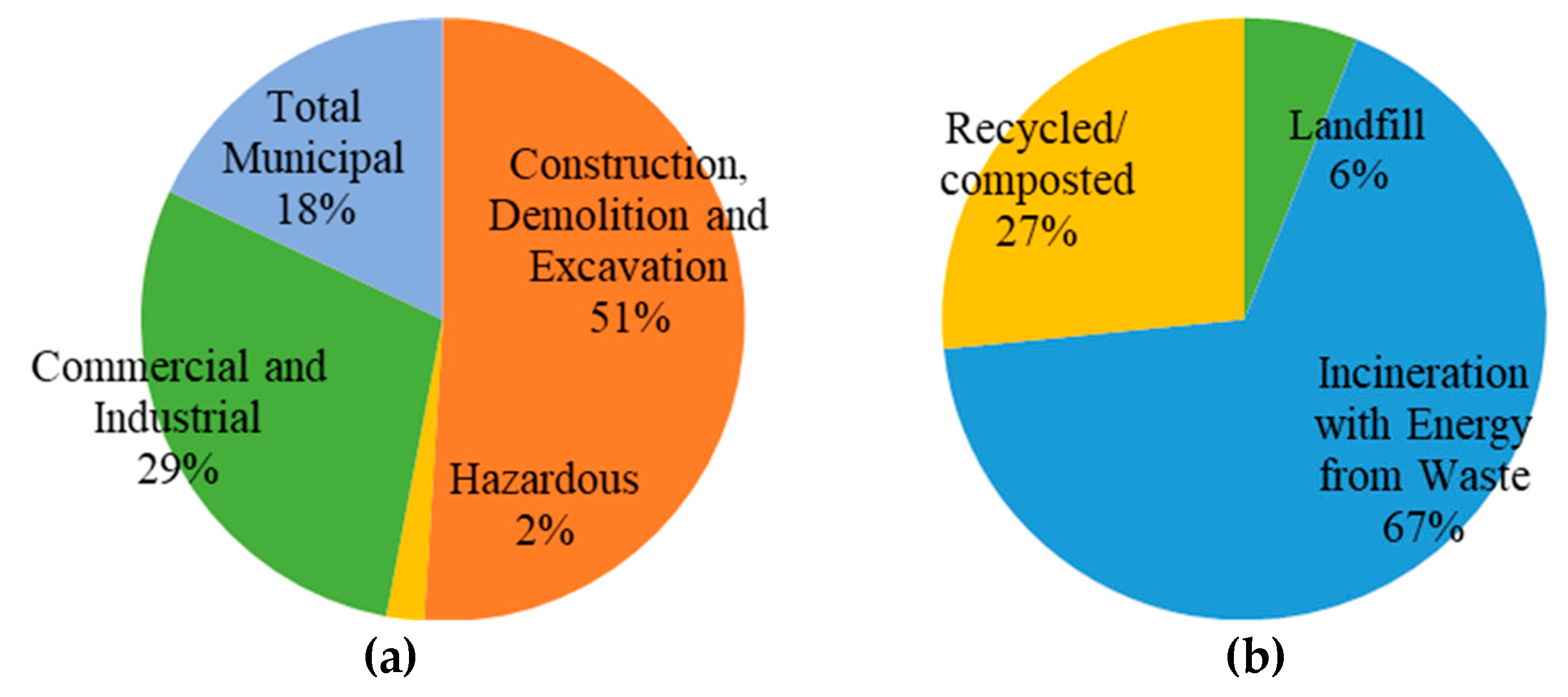
Tyseley Energy Park (TEP) in Birmingham, UK, is a renowned project aiming to adopt and develop sustainable energy generation technologies for the city at a time when its current EfW MSWM contract was due to expire (in 2019). Opportunities to embrace CE arise from such vast amounts of waste being at risk of remaining untreated. The land where the project is to be developed is privately owned and many business tenants are currently settled at the site. Other companies have private interests on settling businesses therein with IS potential and universities are interested in the research opportunities arising around renewable energies. The local government owns the incineration facilities and has a contract with a waste management operator to recover energy from a large portion of the MSW collected in the city, yet there exist general environmental and societal concerns by local inhabitants. Therefore, the local government and related companies have requested the help of consultancy services. This provides an opportunity for embedding CE principles in the development of TEP and there is no reason why this could not materialise if cooperation between stakeholders is achieved. Recent data on the city’s MSWM [52] as depicted in Figure 2 shows that, even though Birmingham has one of the lowest landfill rates in the UK, two-thirds of the MSW is still treated via incineration with energy recovery. Despite annually producing 217 GWh of energy each year, this amount is equivalent to just over 1% of the city’s total energy demand [52]. This casts doubt on the true circularity of the current treatment, and suggests that opportunities for improving the city’s MSWM to be more aligned to CE principles could be generated and should be embraced.

3.2. STEP 1: Scope of study and stakeholders for TEP, Birmingham

3.2.1. Step 1a: Scope of the Study

Drawing on the description in the previous section, the scope of this study is to compare CE MSWM future scenarios for TEP, Birmingham. The primary influencing factor is that the current EfW plant in Tyseley is due to close, and CE opportunities arising from this have been widely discussed in meetings with the city stakeholders. The Birmingham case study is an academic exercise using a sub-set of real decision-makers from an ongoing process. The authors have performed solely as external observers, although the outcomes are being shared with the wider set of decision-makers.

3.2.2. Step 1b: Stakeholder Selection

The respondents in this study included a consultant in ISs, a university researcher on CE SMEs, a Tyseley ward local (community) representative, a steel sector company landowner in TEP, and a representative of Birmingham and Solihull Local Enterprise Partnership (representing local government). Drawing on the previous description of the problem and its elements, the respondents’ identities and any information that could enable them to be traced back is not revealed and they were thus categorised in stakeholder groups as follows:

• Companies—energy sector businesses in the TEP
• Academic institutions
• Local government
• General public
• Consultants—externals to the previous stakeholders who provide consultation services

3.3. STEP 2: Indicators selection and formulation of CE MSWM Scenarios

3.3.1. Step 2a: Indicators Selection

Applying Step 2 of the methodology (Section 2.2), the selected indicators for the case study are shown in

Table 1. Indicators adopted for the evaluation of Circular Economy (CE) waste management scenarios.

No.	Indicator	Unit	Description	Objective
1	Investment cost	£M/yr	It is the £million invested in a project.	Minimise
2	GVA 1 impact	£M/yr	It measures the total annual added production value at the end of the year.	Maximise
3	Payback	months	It indicates the time required for a project to recover the investment.	Minimise
4	Carbon emissions mitigation	CO2 kt/yr	It reflects the amount of CO2 emissions in kilotonnes that are reduced/saved yearly.	Maximise
5	MSW generation reduction	%	It measures the MSW generated in comparison to a previous year.	Maximise
6	Recycling rate of MSW	%	It measures the recycling rate of MSW, and the level of materials re-used and recycled in the city.	Maximise
7	Landfill rate of MSW	%	It measures the rate of MSW that is not diverted from disposal in the city.	Minimise
8	Jobs creation	#	It measures new jobs created per annum.	Maximise
9	Public awareness and satisfaction	%	It expresses the overview of opinions related to the MSWM system by the local population.	Maximise

¹ GVA—Gross Value Added.

. They have been selected through an extensive and thorough literature review. Their choice was based on being understandable, pragmatic, relevant, representative and able to assess a sustainability dimension (i.e., they all comply with the five recommended properties, see Section 2.2.1) and are deemed appropriate to the scale (i.e., city and eco-industrial park levels). In order to study the three acknowledged dimensions of CE and sustainability, three main indicator categories were selected (i.e., economic (indicators 1 to 3), environmental (indicators 4 to 7) and social (indicators 8 and 9). The appropriate units of measure and underpinning objective of the indicator (i.e., to minimise versus maximise the quantity) are shown. For example, indicator 1, Investment cost, is one of the most commonly used economic indicators [53]. It was set to be minimised, in line with Behera et al.’s [54] framework arguing that research performed in EIPs (as in TEP) is meant to be developed into a business (profit-led activities), thus aiming to reduce costs.

3.3.2. Step 2b: Construct Possible Scenarios

The indicators are used to set performance levels within the future scenarios as shown in

Table 2. Future CE scenarios matrix for Municipal Solid Waste Management (MSWM) in Birmingham, UK.

Type	No.	Indicator	Scenarios				Unit
			MF	PR	NSP	FW
Economic	1	Investment cost	46.4	53.8	60.6	43.1	£M/yr
	2	GVA impact	12.5	15.0	17.0	12.0	£M/yr
	3	Payback	180.0	300.0	360.0	240.0	months
Environmental	4	Carbon emissions mitigation	45.0	55.0	65.0	35.0	CO2 kt/yr
	5	MSW generation reduction	7.0	8.5	10.0	3.0	%
	6	Recycling rate of MSW	31.5	40.0	50.0	30.0	%
	7	Landfill rate of MSW	6.0	2.5	1.0	5.0	%
Social	8	Jobs creation	1157.0	1469.0	1836.0	1101.0	#
	9	Public awareness and satisfaction	44.0	56.0	70.0	42.0	%

. (Note, the user could use more indicators than those shown here; an abridged set is used herein to aid understanding of the method). These values are not predictions but merely suggestions of likely future performance for the year 2030 drawn from data [55,56]. The supporting narrative for these values within each scenario has once again been removed for clarity.

3.4. STEP 3: Subjective Weights for Indicators

3.4.1. Step 3a: Stakeholders Rank Indicators

In this step, the five critical stakeholder groups (shown as A to E in

Table 3. The indicators key on the left and stakeholders’ responses on the right.

Type	No.	Indicator	Rank Value	Stakeholders’ Responses
				A	B	C	D	E
Economic	1	Investment cost	9	1, 3	5	2	1,3	2
	2	GVA impact	8	8	6, 7	8	4, 9	1
	3	Payback	7	9	3	1		3
Environmental	4	Carbon emissions mitigation	6	2	4	4
	5	MSW generation reduction	5	4, 5, 6, 7	1	9		8, 9
	6	Recycling rate of MSW	4		8	3		4
	7	Landfill rate of MSW	3		9	5, 6, 7	2, 5, 6, 7	5, 6, 7
Social	8	Jobs creation	2		2		8
	9	Public awareness and satisfaction	1

) were asked to rank the selected nine indicators (using a priority scale, see Section 2.2.1). Stakeholders were told not to use the same ranking number more than once; however, they were allowed to have more than one indicator with the same level of relevance. For example, stakeholder A and D gave indicators 1 and 3 the highest ranking of 9, likewise stakeholder C and E gave indicators 5, 6 and 7 an equal ranking of 3. None of the stakeholders deemed any indicator to be irrelevant.

3.4.2. Step 3b: Pairwise Comparison of Stakeholder Scores

The priority scale helped the stakeholders to simplify the process of pairwise comparing the selected indicators

Table 4. Example matrix of pairwise comparisons for stakeholder B.

			Column indicators
			Cj
			Investment cost	GVA impact	Payback	Carbon emissions mitigation	MSW generation reduction	Recycling rate of MSW	Landfill rate of MSW	Jobs creation	Public awareness and satisfaction
Row Indicators			C1	C2	C3	C4	C5	C6	C7	C8	C9
Ri	Investment Cost	R1	1	4	1/3	1/2	1/5	1/4	1/4	2	3
	GVA Impact	R2	1/4	1	1/6	1/5	1/8	1/7	1/7	1/3	1/2
	Payback	R3	3	6	1	2	1/3	1/2	1/2	4	5
	Carbon Emissions Mitigation	R4	2	5	1/2	1	1/4	1/3	1/3	3	4
	MSW Generation Reduction	R5	5	8	3	4	1	2	2	6	7
	Recycling Rate of MSW	R6	4	7	2	3	1/2	1	1	5	6
	Landfill Rate of MSW	R7	4	7	2	3	1/2	1	1	5	6
	Jobs Creation	R8	1/2	3	1/4	1/3	1/6	1/5	1/5	1	2
	Public Awareness and Satisfaction	R9	1/3	2	1/5	1/4	1/7	1/6	1/6	1/2	1
ΣCj			20	43	9 4/9	14 2/7	3 2/9	5 3/5	5 3/5	26 5/6	34 1/2

. A pairwise comparison matrix was produced from the filled-in priority scales Table 3 and by applying Equations (1) and (2). It is not possible to show the calculations for all pairwise comparisons of all 9 indicators and all 5 stakeholders, as there would need to be a total of n × (n − 1)/2 comparisons made. Hence, the set of pairwise comparisons for stakeholder B are shown in Table 4. For illustration, calculations associated with indicator 1 (i.e., Investment cost) are shown. For the first calculation, it can be seen from Table 3 (shaded in light grey) that stakeholder B gave Investment cost (${\mathrm{R}}_1$) a value of 5, and again Investment cost (${\mathrm{C}}_1$) a value of 5, hence the value of ${\mathrm{DV}}_{1,1}=1+({\mathrm{R}}_1-{\mathrm{C}}_1)=1+(5-5)=1$, likewise:

$${\mathrm{DV}}_{2,1}=\raisebox{1ex}{$1$}\!\left/ \!\raisebox{-1ex}{$(1+\left|{\mathrm{R}}_2-{\mathrm{C}}_1\right|)$}\right.=\raisebox{1ex}{$1$}\!\left/ \!\raisebox{-1ex}{$(1+\left|2-5\right|)$}\right.=1/4$$

$${\mathrm{DV}}_{3,1}=1+({\mathrm{R}}_3-{\mathrm{C}}_1)=1+(7-5)=3$$

$${\mathrm{DV}}_{4,1}=1+({\mathrm{R}}_4-{\mathrm{C}}_1)=1+(6-5)=2$$

$${\mathrm{DV}}_{5,1}=1+({\mathrm{R}}_5-{\mathrm{C}}_1)=1+(9-5)=5$$

$${\mathrm{DV}}_{6,1}=1+({\mathrm{R}}_6-{\mathrm{C}}_1)=1+(8-5)=4$$

$${\mathrm{DV}}_{7,1}=1+({\mathrm{R}}_7-{\mathrm{C}}_1)=1+(8-5)=4$$

$${\mathrm{DV}}_{8,1}=\raisebox{1ex}{$1$}\!\left/ \!\raisebox{-1ex}{$(1+\left|{\mathrm{R}}_8-{\mathrm{C}}_1\right|)$}\right.=\raisebox{1ex}{$1$}\!\left/ \!\raisebox{-1ex}{$(1+\left|4-5\right|)$}\right.=1/2$$

$${\mathrm{DV}}_{9,1}=\raisebox{1ex}{$1$}\!\left/ \!\raisebox{-1ex}{$(1+\left|{\mathrm{R}}_9-{\mathrm{C}}_1\right|)$}\right.=\raisebox{1ex}{$1$}\!\left/ \!\raisebox{-1ex}{$(1+\left|3-5\right|)$}\right.=1/3$$

It must be noted that the ${\mathrm{DV}}_{\mathrm{i},\mathrm{j}}$ values in the diagonal should be ones, because the comparisons between the indicator in the column minus the indicator in the row results in a subtraction of the exact same indicator plus one. Also, the values below the diagonal (shaded in dark grey) must mirror reciprocally those above it, because these comparisons are between the same indicators, but oppositely.

3.4.3. Step 3c: Determine Subjective Weights from Stakeholders

Using the outputs from Step 3b, the AHP technique is now applied. For illustration, the examples to be used are the shaded cells in

Table 5. Example normalised matrix of pairwise comparisons for stakeholder B.

Row Indicators		${\widehat{\mathbf{C}}}_{\mathbf{j}}$									1st Weights	Iteration 1	2nd Weights
		${\widehat{\mathbf{C}}}_{\mathbf{1}}$	${\widehat{\mathbf{C}}}_{\mathbf{2}}$	${\widehat{\mathbf{C}}}_{\mathbf{3}}$	${\widehat{\mathbf{C}}}_{\mathbf{4}}$	${\widehat{\mathbf{C}}}_{\mathbf{5}}$	${\widehat{\mathbf{C}}}_{\mathbf{6}}$	${\widehat{\mathbf{C}}}_{\mathbf{7}}$	${\widehat{\mathbf{C}}}_{\mathbf{8}}$	${\widehat{\mathbf{C}}}_{\mathbf{9}}$
${\widehat{\mathbf{R}}}_{\mathbf{i}}$	${\widehat{\mathbf{R}}}_{\mathbf{1}}$	0.050	0.093	0.035	0.035	0.062	0.045	0.045	0.075	0.087	0.0585	0.5363	0.0568
	${\widehat{\mathbf{R}}}_{\mathbf{2}}$	0.012	0.023	0.018	0.014	0.039	0.026	0.026	0.012	0.014	0.0205	0.1873	0.0198
	${\widehat{\mathbf{R}}}_{\mathbf{3}}$	0.149	0.140	0.106	0.140	0.104	0.089	0.089	0.149	0.145	0.1235	1.1695	0.1240
	${\widehat{\mathbf{R}}}_{\mathbf{4}}$	0.100	0.116	0.053	0.070	0.078	0.060	0.060	0.112	0.116	0.0848	0.7912	0.0839
	${\widehat{\mathbf{R}}}_{\mathbf{5}}$	0.249	0.186	0.317	0.280	0.311	0.358	0.358	0.224	0.203	0.2761	2.6173	0.2774
	${\widehat{\mathbf{R}}}_{\mathbf{6}}$	0.199	0.163	0.212	0.210	0.155	0.179	0.179	0.186	0.174	0.1841	1.7553	0.1861
	${\widehat{\mathbf{R}}}_{\mathbf{7}}$	0.199	0.163	0.212	0.210	0.155	0.179	0.179	0.186	0.174	0.1841	1.7553	0.1861
	${\widehat{\mathbf{R}}}_{\mathbf{8}}$	0.025	0.070	0.026	0.023	0.052	0.036	0.036	0.037	0.058	0.0403	0.3661	0.0388
	${\widehat{\mathbf{R}}}_{\mathbf{9}}$	0.017	0.047	0.021	0.018	0.044	0.030	0.030	0.019	0.029	0.0282	0.2554	0.0271
Σ${\widehat{\mathbf{C}}}_{\mathbf{j}}$		1.000	1.000	1.000	1.000	1.000	1.000	1.000	1.000	1.000	1.0000	9.4337	1.0000

. First, the normalised matrix of pairwise comparisons is calculated using Equation (3) and data from Table 4, the normalised value of the comparison between indicator 1 and indicator 1 is: ${\mathrm{NV}}_{1,1,}=\frac{{\mathrm{DV}}_{1,1}}{{\mathrm{C}}_1}=\frac{1}{20}=0.050$. The process is repeated to fill in the table. Second, the first weight for indicator 1 can be obtained using Equation (4), being the arithmetic mean of the row of indicator 1 (${\widehat{\mathrm{R}}}_{\mathrm{i}}$):

$${\mathrm{I}}_1=\frac{1}{9}{\sum }_{\mathrm{i}=1}^9{\mathrm{NV}}_{\mathrm{i}}=\frac{1}{9}(0.500+0.93+0.035+0.035+0.062+0.045+0.075+0.087)=0.0585$$

This 0.0585 value represents, on a scale from zero to one, how much stakeholder B considers indicator 1 to be worth in comparison with the rest of the indicators. To find the exact weights, several iterations must be performed. For illustration, only the first iteration is performed. Equation (5) is applied to multiply the 1^st weight’s vector by the original matrix of pairwise comparisons (Table 4). Thus, the revised (weight) value for indicator 1 (${\mathrm{RV}}_1$) is given by: ${\mathrm{RV}}_1={\sum }_{\mathrm{i}=1}^9({\mathrm{I}}_{\mathrm{i}}\times {\mathrm{DV}}_{1,\mathrm{j}})={\mathrm{I}}_1\times {\mathrm{DV}}_{1,1}+{\mathrm{I}}_2\times {\mathrm{DV}}_{1,2}+{\mathrm{I}}_3\times {\mathrm{DV}}_{1,3}+{\mathrm{I}}_4\times {\mathrm{DV}}_{1,4}+{\mathrm{I}}_5\times {\mathrm{DV}}_{1,5}+{\mathrm{I}}_6\times {\mathrm{DV}}_{1,6}+{\mathrm{I}}_7\times {\mathrm{DV}}_{1,7}+{\mathrm{I}}_8\times {\mathrm{DV}}_{1,8}+{\mathrm{I}}_9\times {\mathrm{DV}}_{1,9}$:

$$\begin{array}{c}{\mathrm{RV}}_1=0.0585\times 1+0.0205\times 4+0.1235\times \frac{1}{3}+0.0848\times \frac{1}{2}+0.2761\times \frac{1}{5}+0.1841\times \frac{1}{4}+0.1841\times \frac{1}{4}\\ +0.0403\times 2+0.0282\times 3=0.5363\end{array}$$

With the revised values, they must be normalised using Equation (6). Thus, this gives the second weight value for indicator 1: ${\check{\mathrm{I}}}_1=\frac{{\mathrm{RV}}_1}{{\mathrm{RV}}_{\mathrm{i}}}=\frac{0.5363}{9.4337}=0.0568$.

Note that the sum of the indicator weights must be equal to one. The process iterates until the newly calculated weights are not significantly different to those previously computed. The final subjective weight vectors for all five stakeholders are shown in

Table 6. Subjective weight vectors for stakeholders.

Type	No.	Indicator	Stakeholders
			A	B	C	D	E
Economic	1	Investment cost	0.2465	0.0564	0.1540	0.2518	0.2282
	2	GVA impact	0.0694	0.0200	0.3132	0.0335	0.3194
	3	Payback	0.2465	0.1232	0.0465	0.2518	0.1614
Environmental	4	Carbon emissions mitigation	0.0412	0.0832	0.1052	0.1701	0.0483
	5	MSW generation reduction	0.0412	0.2799	0.0296	0.0335	0.0304
	6	Recycling rate of MSW	0.0412	0.1858	0.0296	0.0335	0.0304
	7	Landfill rate of MSW	0.0412	0.1858	0.0296	0.0335	0.0304
Social	8	Jobs creation	0.1642	0.0386	0.2217	0.0220	0.0756
	9	Public awareness and satisfaction	0.1087	0.0271	0.0707	0.1701	0.0756
IR			1.1717%	2.4673%	2.6644%	1.3273%	2.5760%

. The bottom row is the IR calculated for the final weights; this will be explained in Section 3.6.1. The calculations were performed with the aid of an adapted Excel template [57].

3.5. STEP 4: Objective Weights for CE MSWM Scenarios

3.5.1. Step 4a: Rescale Scenarios Performance

Before being able to pairwise compare the scenarios, their suggested performances need to be rescaled into the ‘priority scale’ range. However, first, the maximum number of rankings needs to be determined. By substituting in Equation (7): four being the number of scenarios (“x”), and 0.5 the maximum allowed weight for a single scenario (“y”). Thus, three is the maximum times that a scenario is allowed to be more important than another. The number of levels to use (“c”) is three (the top 9 to 7 from the ‘priority scale’):

$$\mathrm{c}=(4-1)/((1/0.5)-1)=3$$

Using Equations (8) and (9), the data for CE scenarios in Table 2 are rescaled and shown in

Table 7. Rescaled suggested performance of CE scenarios.

	Indicators
	Investment Cost	GVA impact	Payback	Carbon Emissions Mitigation	MSW Generation Reduction	Recycling Rate of MSW	Landfill Rate of MSW	Jobs Creation	Public Awareness and Satisfaction
Scenarios	C1	C2	C3	C4	C5	C6	C7	C8	C9
MF	8.6	7.2	9.0	7.7	8.1	7.2	7.0	7.2	7.1
PR	7.8	8.2	7.7	8.3	8.6	8.0	8.4	8.0	8.0
NSP	7.0	9.0	7.0	9.0	9.0	9.0	9.0	9.0	9.0
FW	9.0	7.0	8.3	7.0	7.0	7.0	7.4	7.0	7.0

. For example, for indicator 1, Investment cost, to rescale the scenario values in Table 2 the formula to use is Equation (9) because the objective of the indicator is to be minimised as follows:

$${{\mathrm{MF}}^{\prime }}_1=\frac{43.1-46.4}{43.1-60.6}\times (7-9)+9=8.6$$

$${{\mathrm{PR}}^{\prime }}_1=\frac{43.1-53.8}{43.1-60.6}\times (7-9)+9=7.8$$

$${{\mathrm{NSP}}^{\prime }}_1=\frac{43.1-60.6}{43.1-60.6}\times (7-9)+9=7.0$$

$${{\mathrm{FW}}^{\prime }}_1=\frac{43.1-43.1}{43.1-60.6}\times (7-9)+9=7.0$$

Values in between the levels (top 9 to 7 from the ‘priority scale’) are used, thus the first decimal rounded figure is used for further AHP calculations.

3.5.2. Step 4b: Pairwise Comparison of Scenarios

Similar to pairwise comparison of the stakeholders rankings, the scenarios rescaled performances are pairwise compared using the ‘priority scale’ according to each indicator individually. This process used the output from the previous step

Table 8. Example matrix of pairwise comparisons of scenarios for indicator 1, Investment cost.

Indicator 1: Investment Cost		Column Scenarios
		Cj
Row scenarios		MF	PR	NSP	FW
Ri	MF	1.000	1.800	2.600	0.714
	PR	0.556	1.000	1.800	0.455
	NSP	0.385	0.556	1.000	0.333
	FW	1.400	2.200	3.000	1.000
	ΣCj	3.340	5.556	8.400	2.502

to create the matrices for each indicator. For illustration purposes, only the matrix for indicator 1, Investment cost, is presented in Table 8. The rest of the indicators have their own matrix of pairwise comparisons; while they are not presented in this paper, they follow the same calculating procedure. For the first calculation in Table 8, it can be seen from Table 7 (shaded in light grey) that for indicator 1, Investment cost (C₁) and scenario MF, the rescaled value of the MF scenario is 8.6, and again the rescaled value of the MF scenario is 8.6, hence the difference value is:

$${\mathrm{DV}}_{\mathrm{MF},\mathrm{MF}}=1+({\mathrm{MF}}_1-{\mathrm{MF}}_1)=1+(8.6-8.6)=1.000,\mathrm{likewise}:$$

$${\mathrm{DV}}_{\mathrm{PR},\mathrm{MF}}=\raisebox{1ex}{$1$}\!\left/ \!\raisebox{-1ex}{$(1+\left|{\mathrm{PR}}_1-{\mathrm{MF}}_1\right|)$}\right.=\raisebox{1ex}{$1$}\!\left/ \!\raisebox{-1ex}{$(1+\left|7.8-8.6\right|)$}\right.=0.556$$

$${\mathrm{DV}}_{\mathrm{NSP},\mathrm{MF}}=\raisebox{1ex}{$1$}\!\left/ \!\raisebox{-1ex}{$(1+\left|{\mathrm{NSP}}_1-{\mathrm{MF}}_1\right|)$}\right.=\raisebox{1ex}{$1$}\!\left/ \!\raisebox{-1ex}{$(1+\left|7.0-8.6\right|)$}\right.=0.385$$

$${\mathrm{DV}}_{\mathrm{FW},\mathrm{MF}}=1+({\mathrm{FW}}_1-{\mathrm{MF}}_1)=1+(9.0-8.6)=1.400$$

3.5.3. Step 4c: Determine Objective Weights for Scenarios

The AHP technique is similarly applied to determine the objective weights of scenarios. For illustration, the examples to be used are the shaded cells in

Table 9. Example normalised matrix of pairwise comparisons of CE scenarios for indicator 1.

Row Scenarios		${\widehat{\mathbf{C}}}_{\mathbf{j}}$				1st Weights	Iteration 1	2nd Weights
		${\widehat{\mathbf{C}}}_{\mathbf{MF}}$	${\widehat{\mathbf{C}}}_{\mathbf{PR}}$	${\widehat{\mathbf{C}}}_{\mathbf{NSP}}$	${\widehat{\mathbf{C}}}_{\mathbf{FW}}$
${\widehat{\mathbf{R}}}_{\mathbf{i}}$	${\widehat{\mathbf{R}}}_{\mathbf{MF}}$	0.299	0.324	0.310	0.285	0.3046	1.2231	0.3048
	${\widehat{\mathbf{R}}}_{\mathbf{PR}}$	0.166	0.180	0.214	0.182	0.1856	0.7438	0.1853
	${\widehat{\mathbf{R}}}_{\mathbf{NSP}}$	0.115	0.100	0.119	0.133	0.1169	0.4681	0.1166
	${\widehat{\mathbf{R}}}_{\mathbf{FW}}$	0.419	0.396	0.357	0.400	0.3930	1.5782	0.3933
Σ${\widehat{\mathbf{C}}}_{\mathbf{j}}$		1.000	1.000	1.000	1.000	1.0000	4.0132	1.0000

. First, the normalised matrix of pairwise comparisons is calculated using Equation (3) and data from Table 8. The normalised value of the comparison for indicator 1 between scenario MF and scenario MF is: ${\mathrm{NV}}_{\mathrm{MF},\mathrm{MF}}=\frac{{\mathrm{DV}}_{\mathrm{MF},\mathrm{MF}}}{\sum {\mathrm{C}}_{\mathrm{MF}}}=\frac{1}{3.340}=0.299$. The process is repeated to fill in the table. Second, the first weight for indicator 1 and scenario MF can be obtained using Equation (4), being the arithmetic mean of the row of scenario MF:

$${\mathrm{S}}_{\mathrm{MF},1}=\frac{1}{4}{\displaystyle \sum _{\mathrm{i}=1}^4}{\mathrm{NV}}_{\mathrm{MF},\mathrm{i}}=\frac{1}{4}(0.299+0.324+0.310+0.285)=0.3046$$

To find the exact weights, several iterations must be performed. For illustration, only the first iteration is presented. Equation (5) is applied to multiply the 1^st weight’s vector by the original matrix of pairwise comparisons (Table 8). Thus, the revised weight value for scenario MF and indicator 1 is:

$${\mathrm{RV}}_{\mathrm{MF},1}={\displaystyle \sum _{\mathrm{i}=4}^4}({\mathrm{S}}_{\mathrm{i},1}\times {\mathrm{DV}}_{\mathrm{MF},\mathrm{i}})={\mathrm{S}}_{\mathrm{MF},1}\times {\mathrm{DV}}_{\mathrm{MF},\mathrm{MF}}+{\mathrm{S}}_{\mathrm{PR},1}\times {\mathrm{DV}}_{\mathrm{MF},\mathrm{PR}}+{\mathrm{S}}_{\mathrm{NSP},1}\times {\mathrm{DV}}_{\mathrm{MF},\mathrm{NSP}}+{\mathrm{S}}_{\mathrm{FW},1}\times {\mathrm{DV}}_{\mathrm{MF},\mathrm{FW}}$$

$${\mathrm{RV}}_{\mathrm{MF},1}=0.3046\times 1.000+0.1856\times 1.800+0.1169\times 2.600+0.3930\times 0.714=1.2231$$

The revised values must be normalised using Equation (6). Thus, this gives the second weight value for scenario MF and indicator 1: ${\check{\mathrm{S}}}_{\mathrm{MF},1}=\frac{{\mathrm{RV}}_{\mathrm{MF},1}}{\sum {\mathrm{RV}}_{\mathrm{i}}}=\frac{1.2231}{4.0132}=0.3048$.

Table 10. Objective weight matrix for the CE scenarios.

		Scenarios
Indicators 1		MF	PR	NSP	FW	IR
1	Investment Cost	0.3047	0.1853	0.1167	0.3933	0.3859%
2	GVA Impact	0.1509	0.2781	0.4387	0.1323	0.4302%
3	Payback	0.4182	0.1860	0.1221	0.2736	0.4564%
4	Carbon Emissions Mitigation	0.1860	0.2736	0.4182	0.1221	0.4564%
5	MSW Generation Reduction	0.2108	0.2934	0.3825	0.1132	0.3526%
6	Recycling Rate of MSW	0.1552	0.2580	0.4511	0.1357	0.4420%
7	Landfill Rate of MSW	0.1253	0.2939	0.4200	0.1607	0.4018%
8	Jobs Creation	0.1552	0.2580	0.4511	0.1357	0.4420%
9	Public Awareness and Satisfaction	0.1479	0.2606	0.4534	0.1381	0.4466%
	Total	1.8542	2.2871	3.2539	1.6049

¹ Note that the columns and rows of the matrix have been transposed for presentation purposes.

presents the final objective weight matrix for all four CE scenarios and all nine indicators after the necessary iterations. Each weight represents the performance of the scenario in comparison to the rest of the scenarios for each indicator individually. The rightmost column is the IR calculated for the final weights (this is addressed in Section 3.6.1).

3.6. STEP 5: Ranking Order of the CE Scenarios

3.6.1. Step 5a: Calculate Inconsistency Ratios

The use of the ‘priority scale’ has ensured that there are no inconsistencies in the rankings. However, this must be verified using Equations (10) and (11). For illustration, the IR of the scenarios’ comparison for indicator 1 (${\mathrm{IR}}_1$) will be explained. The final iteration resulted in the maximum Eigenvector or sum of revised values being $\sum {\mathrm{RV}}_1=4.0104$ (very similar to that in the first iteration in Table 9; the matrix dimension is 4; and the RI for a matrix of such dimension is 0.89 (obtained from [41]). Thus, the ${\mathrm{IR}}_1$ is as follows:

$${\mathrm{CI}}_1=\frac{\sum {\mathrm{RV}}_1-\mathrm{k}}{\mathrm{k}-1}=\frac{4.0104-4}{4-1}$$

$${\mathrm{IR}}_1=\frac{{\mathrm{CI}}_1}{{\mathrm{RI}}_4}=\frac{0.0035}{0.89}=0.3859\%$$

All the IR values for both the final subjective and objective weights were presented above in the lowest row and the rightmost column in Table 6 and Table 10, respectively. The IR values are well below the maximum acceptable value (IR < 10%).

3.6.2. Step 5b: Determine preference order of scenarios

To reveal the preference order of the CE scenarios for each stakeholder, the preferability indexes are calculated. Using Equation (12), the indexes for each stakeholder are shown in

Table 11. Preferability indexes and ranking for the CE scenarios for each stakeholder.

Scenarios	Stakeholders
	A	B	C	D	E
MF	0.258	0.208	0.193	0.264	0.232
	(2nd)	(3rd)	(3rd)	(2nd)	(3rd)
PR	0.228	0.263	0.254	0.228	0.239
	(4th)	(2nd)	(2nd)	(4th)	(2nd)
NSP	0.281	0.364	0.374	0.275	0.313
	(1st)	(1st)	(1st)	(1st)	(1st)
FW	0.233	0.164	0.180	0.233	0.215
	(3rd)	(4th)	(4th)	(3rd)	(4th)

, and below them, their ranking order. The sum of the preferability indexes must be 1 for each stakeholder. For example, the preferability index for stakeholder B for the MF scenario (${\mathrm{PI}}_{\mathrm{B},\mathrm{MF}})$ (shaded in light grey in Table 11) is the sum of all the products of each subjective weight $({\mathrm{I}}_{\mathrm{x},\mathrm{n}})$ (shaded in Table 6 multiplied by the objective weight ${\mathrm{S}}_{\mathrm{MF},\mathrm{n}}$ (shaded in Table 10) for the MF scenario and indicator $\mathrm{n}$:

$${\mathrm{PI}}_{\mathrm{B},\mathrm{MF}}={\sum }_{\mathrm{n}=1}^9({\mathrm{I}}_{\mathrm{B},\mathrm{n}}\times {\mathrm{S}}_{\mathrm{MF},\mathrm{n}}),$$

$$\begin{array}{c}{\mathrm{PI}}_{\mathrm{B},\mathrm{MF}}={\mathrm{I}}_{\mathrm{B},1}\times {\mathrm{S}}_{\mathrm{MF},1}+{\mathrm{I}}_{\mathrm{B},2}\times {\mathrm{S}}_{\mathrm{MF},2}+{\mathrm{I}}_{\mathrm{B},3}\times {\mathrm{S}}_{\mathrm{MF},3}+{\mathrm{I}}_{\mathrm{B},4}\times {\mathrm{S}}_{\mathrm{MF},4}+{\mathrm{I}}_{\mathrm{B},5}\times {\mathrm{S}}_{\mathrm{MF},5}+{\mathrm{I}}_{\mathrm{B},6}\times {\mathrm{S}}_{\mathrm{MF},6}\\ +{\mathrm{I}}_{\mathrm{B},7}\times {\mathrm{S}}_{\mathrm{MF},7}+{\mathrm{I}}_{\mathrm{B},8}\times {\mathrm{S}}_{\mathrm{MF},8}+{\mathrm{I}}_{\mathrm{B},9}\times {\mathrm{S}}_{\mathrm{MF},9}\end{array}$$

PI_B,MF = 0.0564 × 0.3047 + 0.0200 × 0.1509 + 0.1232 × 0.4182 + 0.0832 × 0.1860 +
0.2799 × 0.2108 + 0.1858 × 0.1552 + 0.1858 × 0.1253 + 0.0386 × 0.1552 +
0.0271 × 0.1479 = 0.208

3.7. STEP 6: GT Analysis

3.7.1. Step 6a: Use equilibrium Methods

Using the preferences of scenarios above, all their possible combinations for the four CE scenarios and the five stakeholders are calculated (4⁵ = 1024 combinations). For example, using Equation (13) and data from Table 11, the combined preference of stakeholder A to MF, B to FW, C to NSP, D to FW and E to PR is given by:

$${\mathsf{\phi }}_{\mathrm{MF},\mathrm{FW},\mathrm{NSP},\mathrm{FW},\mathrm{PR}}=\sum {\mathrm{PI}}_{\mathrm{A},\mathrm{MF}}+{\mathrm{PI}}_{\mathrm{B},\mathrm{FW}}+{\mathrm{PI}}_{\mathrm{C},\mathrm{NSP}}+{\mathrm{PI}}_{\mathrm{D},\mathrm{FW}}+{\mathrm{PI}}_{\mathrm{E},\mathrm{PR}}$$

$${\mathsf{\phi }}_{\mathrm{MF},\mathrm{FW},\mathrm{NSP},\mathrm{FW},\mathrm{PR}}=\sum 0.258+0.164+0.374+0.233+0.239=1.270$$

The total number of payoffs to be calculated are five (one for each stakeholder) per combined preference (i.e., 1,024 × 5 = 5120 payoffs). For example, from Equation (14), the payoffs vector for the combined preference in the example above is:

$${\prod }_{\mathrm{MF},\mathrm{FW},\mathrm{NSP},\mathrm{FW},\mathrm{PR}}^{\mathrm{A},\mathrm{MF}}={\mathsf{\phi }}_{\mathrm{MF},\mathrm{FW},\mathrm{NSP},\mathrm{FW},\mathrm{PR}}\times {\mathrm{PI}}_{\mathrm{A},\mathrm{MF}}=1.270\times 0.258=0.328$$

$${\prod }_{\mathrm{MF},\mathrm{FW},\mathrm{NSP},\mathrm{FW},\mathrm{PR}}^{\mathrm{B},\mathrm{FW}}={\mathsf{\phi }}_{\mathrm{MF},\mathrm{FW},\mathrm{NSP},\mathrm{FW},\mathrm{PR}}\times {\mathrm{PI}}_{\mathrm{B},\mathrm{FW}}=1.270\times 0.164=0.209$$

$${\prod }_{\mathrm{MF},\mathrm{FW},\mathrm{NSP},\mathrm{FW},\mathrm{PR}}^{\mathrm{C},\mathrm{NSP}}={\mathsf{\phi }}_{\mathrm{MF},\mathrm{FW},\mathrm{NSP},\mathrm{FW},\mathrm{PR}}\times {\mathrm{PI}}_{\mathrm{C},\mathrm{NSP}}=1.270\times 0.374=0.475$$

$${\prod }_{\mathrm{MF},\mathrm{FW},\mathrm{NSP},\mathrm{FW},\mathrm{PR}}^{\mathrm{D},\mathrm{FW}}={\mathsf{\phi }}_{\mathrm{MF},\mathrm{FW},\mathrm{NSP},\mathrm{FW},\mathrm{PR}}\times {\mathrm{PI}}_{\mathrm{D},\mathrm{FW}}=1.270\times 0.233=0.296$$

$${\prod }_{\mathrm{MF},\mathrm{FW},\mathrm{NSP},\mathrm{FW},\mathrm{PR}}^{\mathrm{E},\mathrm{PR}}={\mathsf{\phi }}_{\mathrm{MF},\mathrm{FW},\mathrm{NSP},\mathrm{FW},\mathrm{PR}}\times {\mathrm{PI}}_{\mathrm{E},\mathrm{PR}}=1.270\times 0.239=0.304$$

$${\prod }_{\mathrm{MF},\mathrm{FW},\mathrm{NSP},\mathrm{FW},\mathrm{PR}}=[0.328,0.209,0.475,0.296,0.304],$$

The NCGT equilibrium analysis of payoffs for the stakeholders is performed using the open-access software Gambit (Version 15.1.1, The Gambit Project, Norwich, UK). These payoffs are a representation of the level of satisfaction obtained by each stakeholder for that specific combination of alternative scenarios. Thus, it is of great relevance to uncover the set or the single combination of scenarios which brings an equilibrium to the interactive decision-making. This means finding the highest possible satisfaction to each stakeholder without decreasing that obtained by others. The results in

Table 12. Nash Equilibriums for the combined preferences of stakeholders.

Equilibrium Methods	Nash Equilibriums Found	Stakeholders
		A	B	C	D	E
Pure strategy Equilibria	1	NSP	NSP	NSP	NSP	NSP
		0.453	0.585	0.602	0.442	0.504
Minimising Lyapunov Function	0	-	-	-	-	-
		-	-	-	-	-
Global Newton Tracing	1	NSP	NSP	NSP	NSP	NSP
		0.453	0.585	0.602	0.442	0.504
Solving Systems of Polynomial Equations	1	NSP	NSP	NSP	NSP	NSP
		0.453	0.585	0.602	0.442	0.504

show that, as initially expected, the calculated Nash equilibrium for the majority of the methods is when all stakeholders select the same NSP scenario (${\prod }_{\mathrm{NSP},\mathrm{NSP}.\mathrm{NSP},\mathrm{NSP},\mathrm{NSP}}$). The payoffs are shown in the row below the scenarios.

3.7.2. Step 6b: Apply Allocation Method

Once the Nash equilibrium is identified, the next step is to analyse how stakeholders should arrange their satisfaction levels to prevent them from abandoning their (presumably) cooperative behaviour. This is done by applying CGT allocation methods, which aim to distribute benefits fairly to stakeholders in pre-emptive coalitions to protect cooperation.

For example, using Equation (15), the benefits of coalition ABCDE (where all stakeholders cooperate and are allocated benefits) for the equilibrium result where all stakeholders select the NSP scenario (${\prod }_{\mathrm{NSP},\mathrm{NSP}.\mathrm{NSP},\mathrm{NSP},\mathrm{NSP}}$) is as follows:

$${\prod }_{\mathrm{NSP},\mathrm{NSP},\mathrm{NSP},\mathrm{NSP},\mathrm{NSP}}=[0.453,0.585,0.602,0.442,0.504]$$

$${{\displaystyle \overline{\prod }}}_{\mathrm{NSP},\mathrm{NSP},\mathrm{NSP},\mathrm{NSP},\mathrm{NSP}}=0.517$$

$${\mathsf{\beta }}_{\mathrm{NSP},\mathrm{NSP},\mathrm{NSP},\mathrm{NSP},\mathrm{NSP}}^{\mathrm{A},\mathrm{NSP}}=\sum {{\displaystyle \overline{\prod }}}_{\mathrm{NSP},\mathrm{NSP},\mathrm{NSP},\mathrm{NSP},\mathrm{NSP}}\times {\prod }_{\mathrm{NSP},\mathrm{NSP},\mathrm{NSP},\mathrm{NSP},\mathrm{NSP},\mathrm{NSP}}^{\mathrm{A},\mathrm{NSP}}=0.517\times 0.453=0.234$$

$${\mathsf{\beta }}_{\mathrm{NSP},\mathrm{NSP},\mathrm{NSP},\mathrm{NSP},\mathrm{NSP}}^{\mathrm{B},\mathrm{NSP}}=\sum {{\displaystyle \overline{\prod }}}_{\mathrm{NSP},\mathrm{NSP},\mathrm{NSP},\mathrm{NSP},\mathrm{NSP}}\times {\prod }_{\mathrm{NSP},\mathrm{NSP},\mathrm{NSP},\mathrm{NSP},\mathrm{NSP},\mathrm{NSP}}^{\mathrm{B},\mathrm{NSP}}=0.517\times 0.585=0.302$$

$${\mathsf{\beta }}_{\mathrm{NSP},\mathrm{NSP},\mathrm{NSP},\mathrm{NSP},\mathrm{NSP}}^{\mathrm{C},\mathrm{NSP}}=\sum {{\displaystyle \overline{\prod }}}_{\mathrm{NSP},\mathrm{NSP},\mathrm{NSP},\mathrm{NSP},\mathrm{NSP}}\times {\prod }_{\mathrm{NSP},\mathrm{NSP},\mathrm{NSP},\mathrm{NSP},\mathrm{NSP},\mathrm{NSP}}^{\mathrm{C},\mathrm{NSP}}=0.517\times 0.602=0.311$$

$${\mathsf{\beta }}_{\mathrm{NSP},\mathrm{NSP},\mathrm{NSP},\mathrm{NSP},\mathrm{NSP}}^{\mathrm{D},\mathrm{NSP}}=\sum {{\displaystyle \overline{\prod }}}_{\mathrm{NSP},\mathrm{NSP},\mathrm{NSP},\mathrm{NSP},\mathrm{NSP}}\times {\prod }_{\mathrm{NSP},\mathrm{NSP},\mathrm{NSP},\mathrm{NSP},\mathrm{NSP},\mathrm{NSP}}^{\mathrm{D},\mathrm{NSP}}=0.517\times 0.442=0.229$$

$${\mathsf{\beta }}_{\mathrm{NSP},\mathrm{NSP},\mathrm{NSP},\mathrm{NSP},\mathrm{NSP}}^{\mathrm{E},\mathrm{NSP}}=\sum {{\displaystyle \overline{\prod }}}_{\mathrm{NSP},\mathrm{NSP},\mathrm{NSP},\mathrm{NSP},\mathrm{NSP}}\times {\prod }_{\mathrm{NSP},\mathrm{NSP},\mathrm{NSP},\mathrm{NSP},\mathrm{NSP},\mathrm{NSP}}^{\mathrm{E},\mathrm{NSP}}=0.517\times 0.504=0.260$$

$${\mathsf{\beta }}_{\mathrm{NSP},\mathrm{NSP},\mathrm{NSP},\mathrm{NSP},\mathrm{NSP}}=[0.234,0.302,0.311,0.229,0.260]$$

The rightmost column in

Table 13. Coalitions of stakeholders for obtained Nash equilibrium.

	Payoffs ∏NSP,NSP,NSP,NSP,NSP						Benefits βNSP,NSP,NSP,NSP,NSP
Coalition Name	A	B	C	D	E	${\displaystyle \overline{\mathbf{\prod }}}$	A	B	C	D	E	Σβ
	NSP	NSP	NSP	NSP	NSP		NSP	NSP	NSP	NSP	NSP
A	0.453	0	0	0	0	0.453	0.205	0	0	0	0	0.205
B	0	0.585	0	0	0	0.585	0	0.342	0	0	0	0.342
C	0	0	0.602	0	0	0.602	0	0	0.362	0	0	0.362
D	0	0	0	0.442	0	0.442	0	0	0	0.196	0	0.196
E	0	0	0	0	0.504	0.504	0	0	0	0	0.254	0.254
AB	0.453	0.585	0	0	0	0.519	0.235	0.303	0	0	0	0.538
AC	0.453	0	0.602	0	0	0.527	0.239	0	0.317	0	0	0.556
AD	0.453	0	0	0.442	0	0.447	0.202	0	0	0.198	0	0.400
AE	0.453	0	0	0	0.504	0.478	0.216	0	0	0	0.241	0.457
BC	0	0.585	0.602	0	0	0.593	0	0.347	0.357	0	0	0.704
BD	0	0.585	0	0.442	0	0.514	0	0.300	0	0.227	0	0.527
BE	0	0.585	0	0	0.504	0.544	0	0.318	0	0	0.274	0.592
CD	0	0	0.602	0.442	0	0.522	0	0	0.314	0.231	0	0.545
CE	0	0	0.602	0	0.504	0.553	0	0	0.332	0	0.278	0.610
DE	0	0	0	0.442	0.504	0.473	0	0	0	0.209	0.238	0.447
ABC	0.453	0.585	0.602	0	0	0.546	0.247	0.320	0.329	0	0	0.896
ABD	0.453	0.585	0	0.442	0	0.493	0.223	0.289	0	0.218	0	0.730
ABE	0.453	0.585	0	0	0.504	0.514	0.232	0.300	0	0	0.259	0.791
ACD	0.453	0	0.602	0.442	0	0.499	0.226	0	0.300	0.221	0	0.747
ACE	0.453	0	0.602	0	0.504	0.519	0.235	0	0.312	0	0.262	0.809
ADE	0.453	0	0	0.442	0.504	0.466	0.211	0	0	0.206	0.235	0.652
BCD	0	0.585	0.602	0.442	0	0.543	0	0.318	0.327	0.240	0	0.885
BCE	0	0.585	0.602	0	0.504	0.563	0	0.330	0.339	0	0.284	0.953
BDE	0	0.585	0	0.442	0.504	0.510	0	0.298	0	0.226	0.257	0.781
CDE	0	0	0.602	0.442	0.504	0.516	0	0	0.310	0.228	0.260	0.798
ABCD	0.453	0.585	0.602	0.442	0	0.520	0.235	0.304	0.313	0.230	0	1.082
ABCE	0.453	0.585	0.602	0	0.504	0.536	0.242	0.313	0.322	0	0.270	1.147
ABDE	0.453	0.585	0	0.442	0.504	0.496	0.224	0.290	0	0.219	0.250	0.983
ACDE	0.453	0	0.602	0.442	0.504	0.500	0.226	0	0.301	0.221	0.252	1.000
BCDE	0	0.585	0.602	0.442	0.504	0.533	0	0.312	0.321	0.236	0.269	1.138
ABCDE	0.453	0.585	0.602	0.442	0.504	0.517	0.234	0.302	0.311	0.229	0.260	1.336

shows the sum of the benefits for each coalition, or the total worth of the coalition. It is essential to analyse every possible coalition that can be formed, i.e., from stakeholders working individually to the case where all of them behave cooperatively. Table 13 presents all the possible coalitions to be formed and their ${\mathsf{\beta }}_{\mathrm{NSP},\mathrm{NSP},\mathrm{NSP},\mathrm{NSP},\mathrm{NSP}}$ benefits.

The Shapley value results are shown in

Table 14. Shapley value results for the benefits of stakeholders.

	Benefits βNSP,NSP,NSP,NSP,NSP
Allocation Method	Stakeholders					Σβ
	A	B	C	D	E
Shapley value	0.200	0.337	0.355	0.191	0.253	1.336
	(D)	(I)	(I)	(D)	(D)

. The fairest allocation of benefits corresponds to the five-stakeholder coalition, in other words, when they decide to cooperate and remain in the previously agreed alliance. The letter below each allocated benefit in Table 14 indicates whether it should stay the same (S), increase (I) or decrease (D) compared to the originally claimed benefits in the coalition in Table 13. The sum of the newly proposed distribution must be equal to the total worth of the original coalition. The implications of these results are discussed in Section 4.

4. Discussion

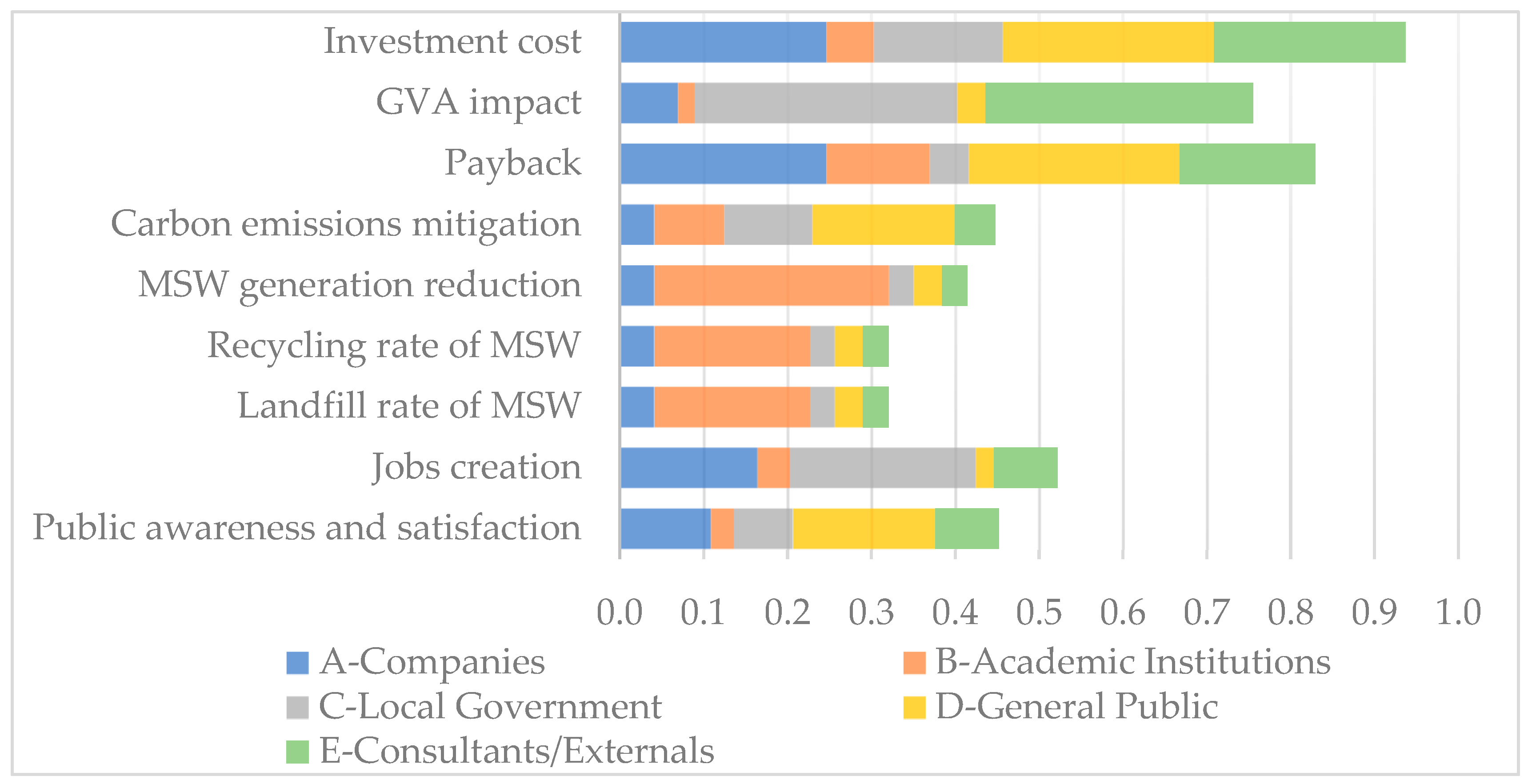
The total subjective weights for the indicators is depicted in Figure 3, in which it can be seen that the environmental indicators have resulted as of the least concern. Previous findings [9] indicate that industry stakeholders prefer economic indicators, whilst municipalities consider environmental indicators as being more important. For this case study, recycling and landfill rates of MSW have yielded the lowest weighted values, whereas the economic indicators resulted in the highest weight values. Academic institutions are the most concerned with environmental indicators. The slightly higher value for the reduction of carbon emissions might be related to the fact that Birmingham is committed to reduce its carbon footprint by 60% by 2027 [55,58,59].

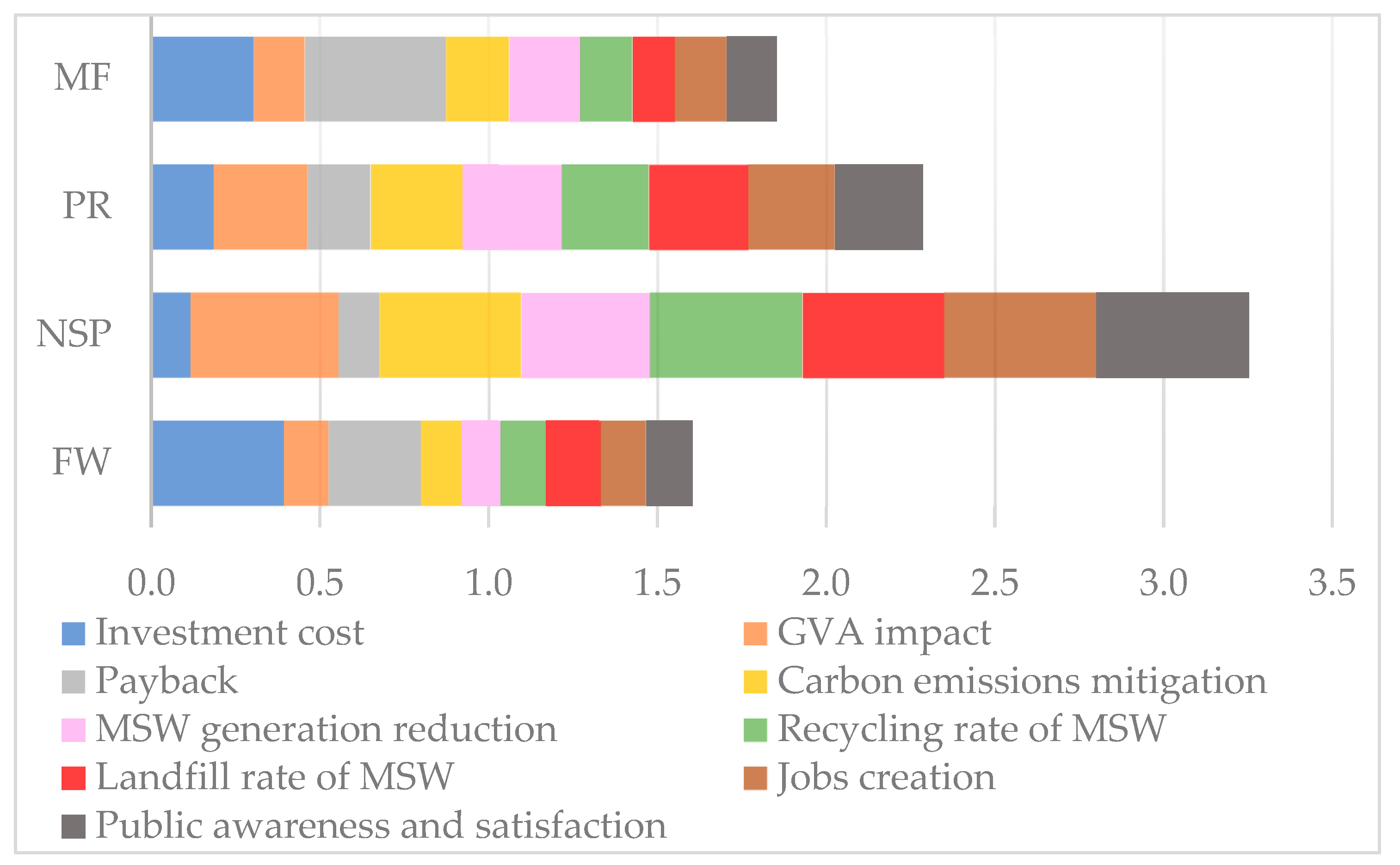
An unexpected finding is the low subjective weight for the Jobs creation indicator for the General Public stakeholder (D). As mentioned by them during the interview: ‘(…) it’s not just about jobs creation, we need skilled jobs in the area, not simple jobs (…)’. Conversely, the most important indicators for the rest of the stakeholders were Investment cost and Payback. This reinforces the initial expectations that the stakeholders’ conflicting viewpoints might be a barrier to cooperate and thus reach the optimal scenario. The scenario that scored highest was NSP, followed by PR; MF was ranked third and the FW scenario resulted as the lowest ranked of all (Figure 4).

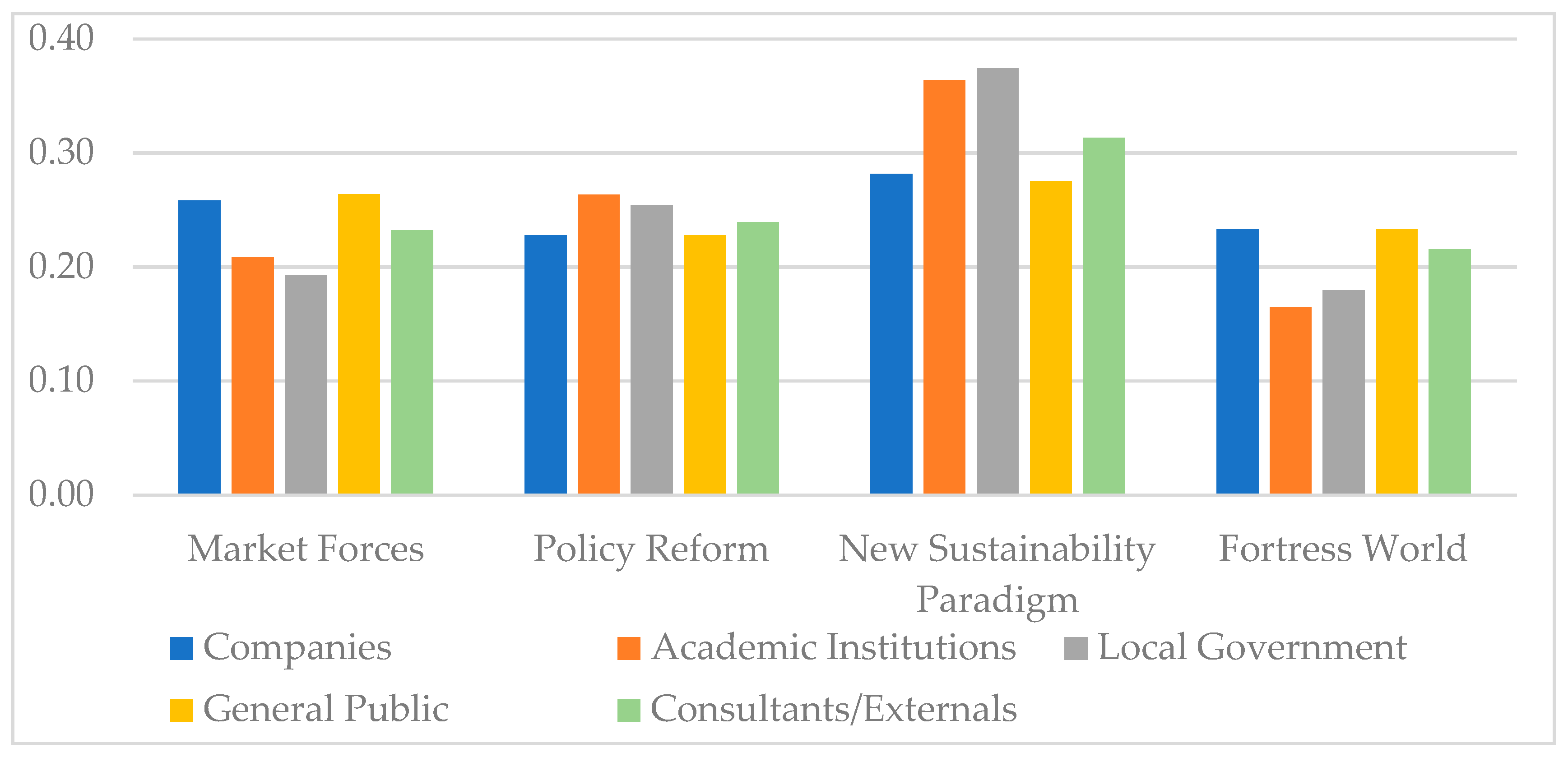
NSP also resulted as the most preferred scenario for all stakeholders (Figure 5). This is in line with previous observations where 70% or their interviewed stakeholders ranked highest the most sustainable performing composting plant site alternative [15]. However, the second most preferred scenario varied between stakeholders. For example: stakeholders A (Companies) and D (General Public) ranked MF, FW and PR in second, third and fourth places, respectively. This means that they prefer a business-as-usual and a breakdown scenario over a strong policy implementation. In contrast, stakeholders B, C and E ranked PR, MF and FW in decreasing order. This suggested, before the GT analysis, that stakeholders having NSP as their most preferred scenario would be willing to work jointly towards it. However, it does not necessarily mean that their priorities are aligned, and that cooperation would occur naturally.

After the preferences of the stakeholders to the CE scenarios were revealed, the NCGT analysis reported that, as expected, stakeholders achieve their maximum levels of satisfaction (payoff) when all four of them select the NSP scenario, meaning this is a Nash equilibrium. If any of the participants were to deviate from this selection unilaterally, not only would that result in a decrease for them, but it would also result in a decrease to the rest of the stakeholders. This combined set of preferences (∏_{NSP,NSP,NSP,NSP,NSP}) was then used to calculate the benefits system for the stakeholders (β_{NSP,NSP,NSP,NSP,NSP}) to enable the CGT analysis to be carried out.

The first row in

Table 15. Coalition distributions of benefits for stakeholders.

	Benefits βNSP,NSP,NSP,NSP,NSP
Coalition	Stakeholders					Σβ
	A	B	C	D	E
Independently	0.205	0.342	0.362	0.196	0.254
ABCDE	0.234	0.302	0.311	0.229	0.260	1.336
	(I)	(D)	(D)	(I)	(I)
Shapley value	0.200	0.337	0.355	0.191	0.253	1.336
	(D)	(I)	(I)	(D)	(D)

indicates the benefits each stakeholder would obtain separately. This implies there is no cooperation, and thus why there is no addition in the rightmost column. The second row shows the benefits obtained by each stakeholder if they all join a coalition and cooperate, with the letters below each entry showing how the benefits obtained compared to the previous benefits—some stakeholders (A, D and E) can increase their benefits whilst the rest (B and C) exhibit a decrease. In the bottom row, the Shapley value assigns benefits differently, with the letters below indicating how this new allocation compares with the previous case in which all stakeholders cooperate (ABCDE).

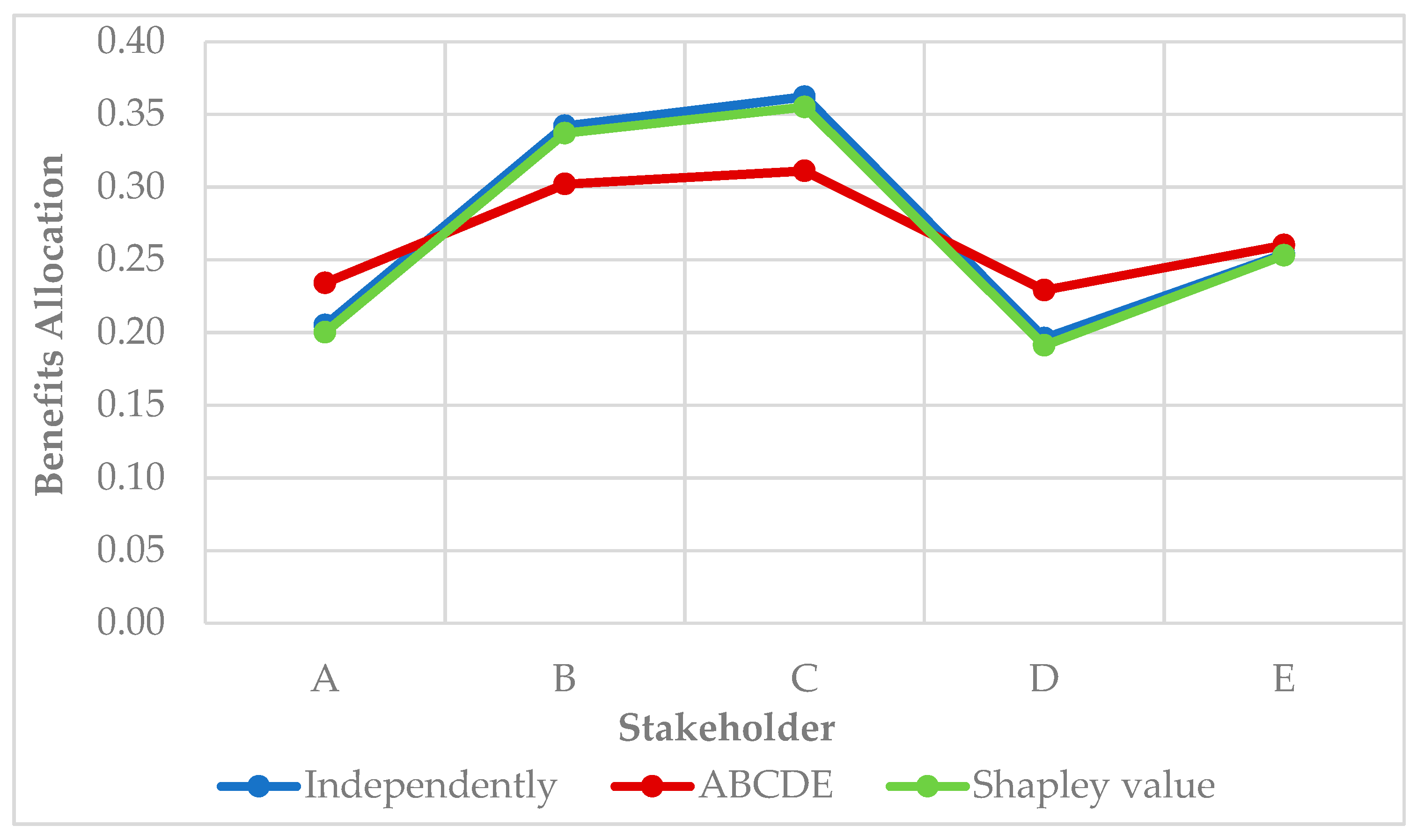
The Shapley value results in lower assignations to all stakeholders than if they work on their own (i.e., when a single stakeholder is considered in five different coalitions, shown in the first row in Table 15). Compared to the values for the ABCDE coalition, the benefit allocation for stakeholders B and C is suggested to increase, because according to the Shapley value definition, their allocation is influenced by their contribution to the coalition. In other words, it is a representation of their bargaining power and, as shown in their independent and ABCDE values, their contributions are the highest. Likewise, Figure 6 helps to visualise these comparisons and shows how the Shapley value is assigning the minimum satisfaction to prevent them from abandoning the coalition.

This is an ideal recommended distribution that would give all stakeholders benefits; otherwise the benefits would only be distributed amongst those who entered a coalition. Some participants (A, D and E) are suggested to decrease their degree of benefit in order to maintain the coalition, since otherwise the other stakeholders might be too unsatisfied with the outcome (their share of the benefits) and believe that their benefits might increase by working on their own (which would not be possible because the entire payoffs model would disintegrate). Thus, some stakeholders are expected to forego a part of their benefits in order that the benefits would be allocated more fairly, while those who contribute more to the coalition can expect to receive higher benefits. This expected increase and decrease of benefits is consistent with previously reported research [60], which show a fair sharing of savings in energy from intercompany heating and cooling integration.

Finally, these results mean that increasing the satisfaction of stakeholders B and C could ensure successful cooperation. To do that it is recommended to trace back those indicators which these stakeholders find more important and work on maximising their performance depending on their objective. For example, by focusing on increasing the GVA impact, despite having little effect on the satisfaction of stakeholder B, it will significantly increase that of stakeholder C. Likewise, reducing further MSW generation increases the satisfaction levels of stakeholder B. It should be noted that these actions do not negatively affect other stakeholders, but will continue contributing to improve their satisfaction levels and thus encourage cooperation towards the NSP scenario [49]. As suggested elsewhere [22], creating equitable benefit and cost distribution to stakeholders in MSWM can increase cooperation and ultimately, the system’s sustainability.

5. Conclusions

Even when stakeholders share a common goal, e.g., adopting Circular Economy (CE), conflicting objectives and priorities between different stakeholders are expected to arise. By providing evidence on stable (equilibrium) and optimal decisions, this paper contributes to the decision-making process by proposing a hybrid methodology that attempts to encourage cooperation between stakeholders to adopt CE principles in Municipal Solid Waste Management (MSWM) in cities. This method facilitates the incorporation of all stakeholders’ views by considering their multiple and sometimes conflicting priorities. It balances the overall decision-making process by harmonising government technical knowledge, private sector profit-led activities and general public needs.

The efficacy of the proposed framework has been demonstrated with a case study of hypothetically built CE scenarios in Tyseley, Birmingham, UK. The five most influential stakeholder groups were identified and asked to rank nine selected CE indicators that measured the performance of four constructed future scenarios. The subjective and objective weights were calculated for the stakeholders and scenarios, respectively, and these were then used to obtain the stakeholders’ preferability indexes and rank their scenarios preferences. The most preferred (or optimal) selection of scenarios was determined using a Nash equilibrium, and the analysis of possible coalitions and the most efficient allocation of benefits was performed using the Shapley value methodology. Thus, the scope of application is to support group decision-making in CE scenarios evaluation, and so it is aimed at the MSWM of cities when multiple stakeholders have different priorities towards future urban scenarios based on CE indicators.

The utilisation of AHP for both the subjective and objective weights not only considers the views and understanding of the stakeholders, but also uses the impartial data of the constructed CE scenarios. The Shapley value allocation of benefits yields a result where all stakeholders share a portion of the benefits; in other words, no coalition where a stakeholder is missing produced an optimal result. However, Cooperative Game Theory (CGT) assumes participants are willing to cooperate and agree on forming coalitions. If stakeholders desert the agreement, the coalition and its benefits model breaks down and jeopardises the possibility of reaching the most preferred, or optimal, scenario.

There are certain factors in decision-making that are extremely difficult to identify and measure; for example, the subjective views on employment in the particular area of Tyseley as briefly presented in the discussions section. In rationality there is no room for human emotions or subjective views. This is a limitation of the proposed method and of Game Theory (GT), as they are both based on the assumptions that actors are intelligent and rational; they have the same information and can make inferences about it, and they will always seek to maximise their utility, respectively. However, in practice, most actors have limited rationality [61] as ”rational decision making” and the “rational planning process” assure; meaning that their decisions are bounded by their limited cognitive capacity, restricted time for decision-making and/or by incomplete information [62]. Whilst the proposed method complies with these GT assumptions, it is acknowledged that they also agree with the criticism from rational decision making because it has been widely debated that decision-making is not always rational [63]. However, rational decision making is widely applied in other social and economic disciplines that fall beyond the scope of this study, and that is why it is not explored in more depth.

The study involved the five most influential actors in the particular TEP site; the results were able to come to a most optimal combined scenario for all participants. While it is relatively uncomplicated to define a comprehensive stakeholder directory, it is difficult to predict whether all actors will continue to comply with GT principles (regarding cooperation and willingness to compromise) later in the decision-making process. In this respect, the proposed framework does not consider multiple stages in the decision-making process or the possibility that new stakeholders might be introduced at later stages of the decision-making process. It is also recommended that future research should attempt to measure the awareness of stakeholders towards CE, their willingness to cooperate (accept/pay) to achieve such a CE transition, their level of trust towards other stakeholders, and their perceptions on their counterparts (e.g., more or less powerful and willing or not to forego benefits to bring fairer distributions).

The proposed methodological framework attempts to provide evidence of how the joint selection of the most sustainable scenario could lead to its realisation, and consequently, formulate recommendations to successfully achieve it. It certainly is not the solution to complicated decision-making processes; however, it facilitates them by making the difficult decisions more transparent. In essence, the method represents a single stage of the decision-making process, where it is necessary to converge on a preferred scenario by adjusting the stakeholder satisfaction levels whilst enhancing indicator performance and without damaging the overall decision-making process. However, negotiations might still be fruitless without extensive communication and the development of a common understanding between stakeholders. It is, therefore, recommended that such an investment of prior effort and meticulous preparation through adoption of this methodology is likely to lead to the CE outcomes to which we all already do, or should, aspire.

References

- Palafox-Alcantar, P.G.; Lee, S.E.; Bouch, C.; Hunt, D.V.L.; Rogers, C.D.F. The Little Book of Circular Economy in Cities; Imagination Lancaster: Lancaster, UK, 2017; ISBN 978-0-70442-950-5. [Google Scholar]
- Palafox-Alcantar, P.G.; Hunt, D.V.L.; Rogers, C.D.F. The complementary use of game theory for the circular economy: A review of waste management decision-making methods in civil engineering. Waste Manag. 2020, 102, 598–612. [Google Scholar] [CrossRef] [PubMed]
- Rogers, C.D.F. Engineering Future Liveable, Resilient, Sustainable Cities Using Foresight. Proc. Inst. Civ. Eng. Eng. 2018, 171, 3–9. [Google Scholar] [CrossRef] [Green Version]
- Circle Economy. The Circularity Gap Report; European Union: Amsterdam, Netherlands, 2018. [Google Scholar]
- Kirchherr, J.; Piscicelli, L.; Bour, R.; Kostense-Smit, E.; Muller, J.; Huibrechtse-Truijens, A.; Hekkert, M. Barriers to the Circular Economy: Evidence from the European Union (EU). Ecol. Econ. 2018, 150, 264–272. [Google Scholar] [CrossRef] [Green Version]
- Veleva, V.; Bodkin, G. Corporate-entrepreneur collaborations to advance a circular economy. J. Clean. Prod. 2018, 188, 20–37. [Google Scholar] [CrossRef]
- Lee, D.H. Econometric assessment of bioenergy development. Int. J. Hydrogen Energy 2017, 42, 27701–27717. [Google Scholar] [CrossRef]
- Kastner, C.A.; Lau, R.; Kraft, M. Quantitative tools for cultivating symbiosis in industrial parks: A literature review. Appl. Energy 2015, 155, 599–612. [Google Scholar] [CrossRef]
- Soltani, A.; Sadiq, R.; Hewage, K. Selecting sustainable waste-to-energy technologies for municipal solid waste treatment: A game theory approach for group decision-making. J. Clean. Prod. 2016, 113, 388–399. [Google Scholar] [CrossRef]
- Luo, M.; Song, X.; Hu, S.; Chen, D. Towards the sustainable development of waste household appliance recovery systems in China: An agent-based modeling approach. J. Clean. Prod. 2019, 220, 431–444. [Google Scholar] [CrossRef]
- Friedrich, E.; Trois, C. Current and future greenhouse gas (GHG) emissions from the management of municipal solid waste in the eThekwini Municipality—South Africa. J. Clean. Prod. 2016, 112, 4071–4083. [Google Scholar] [CrossRef]
- Ripa, M.; Fiorentino, G.; Vacca, V.; Ulgiati, S. The relevance of site-specific data in Life Cycle Assessment (LCA). The case of the municipal solid waste management in the metropolitan city of Naples (Italy). J. Clean. Prod. 2017, 142, 445–460. [Google Scholar] [CrossRef]
- Fei, F.; Wen, Z.; Huang, S.; De Clercq, D. Mechanical biological treatment of municipal solid waste: Energy efficiency, environmental impact and economic feasibility analysis. J. Clean. Prod. 2018, 178, 731–739. [Google Scholar] [CrossRef]
- Estay-Ossandon, C.; Mena-Nieto, A.; Harsch, N. Using a fuzzy TOPSIS-based scenario analysis to improve municipal solid waste planning and forecasting: A case study of Canary archipelago (1999–2030). J. Clean. Prod. 2018, 176, 1198–1212. [Google Scholar] [CrossRef]
- De Feo, G.; De Gisi, S. Using an innovative criteria weighting tool for stakeholders involvement to rank MSW facility sites with the AHP. Waste Manag. 2010, 30, 2370–2382. [Google Scholar] [CrossRef] [PubMed]
- Soltani, A.; Hewage, K.; Reza, B.; Sadiq, R. Multiple stakeholders in multi-criteria decision-making in the context of Municipal Solid Waste Management: A review. Waste Manag. 2015, 35, 318–328. [Google Scholar] [CrossRef] [PubMed]
- Li, N.; Zhao, H. Performance evaluation of eco-industrial thermal power plants by using fuzzy GRA-VIKOR and combination weighting techniques. J. Clean. Prod. 2016, 135, 169–183. [Google Scholar] [CrossRef]
- Sabaghi, M.; Mascle, C.; Baptiste, P. Evaluation of products at design phase for an efficient disassembly at end-of-life. J. Clean. Prod. 2016, 116, 177–186. [Google Scholar] [CrossRef]
- Kaźmierczak, U.; Blachowski, J.; Górniak-Zimroz, J. Multi-Criteria Analysis of Potential Applications of Waste from Rock Minerals Mining. Appl. Sci. 2019, 9, 441. [Google Scholar] [CrossRef] [Green Version]
- Strantzali, E.; Aravossis, K.; Livanos, G.A.; Nikoloudis, C. A decision support approach for evaluating liquefied natural gas supply options: Implementation on Greek case study. J. Clean. Prod. 2019, 222, 414–423. [Google Scholar] [CrossRef]
- Grimes-Casey, H.G.; Seager, T.P.; Theis, T.L.; Powers, S.E. A game theory framework for cooperative management of refillable and disposable bottle lifecycles. J. Clean. Prod. 2007, 15, 1618–1627. [Google Scholar] [CrossRef]
- Karmperis, A.C.; Aravossis, K.; Tatsiopoulos, I.P.; Sotirchos, A. Decision support models for solid waste management: Review and game-theoretic approaches. Waste Manag. 2013, 33, 1290–1301. [Google Scholar] [CrossRef]
- Chen, F.; Chen, H.; Guo, D.; Han, S.; Long, R. How to achieve a cooperative mechanism of MSW source separation among individuals—An analysis based on evolutionary game theory. J. Clean. Prod. 2018, 195, 521–531. [Google Scholar] [CrossRef]
- Rogers, C.D.F.; Hunt, D.V.L. Realising visions for future cities: An aspirational futures methodology. Proc. Inst. Civ. Eng. Urban Des. Plan. 2019, 172, 125–140. [Google Scholar] [CrossRef] [Green Version]
- UKCRIC. Evidence Base and Portfolio of Tools and Techniques Underpinning UKCRIC’s Research Capability in Cities; Collaboratorium for Research on Infrastructure and Cities: London, UK, 2019; Available online: www.ukcric.com (accessed on 27 March 2020).
- Bocken, N.; de Pauw, I.; Bakker, C.; van der Grinten, B. Product design and business model strategies for a circular economy. J. Ind. Prod. Eng. 2016, 33, 308–320. [Google Scholar] [CrossRef] [Green Version]
- Rizos, V.; Behrens, A.; van der Gaast, W.; Hofman, E.; Ioannou, A.; Kafyeke, T.; Flamos, A.; Rinaldi, R.; Papadelis, S.; Hirschnitz-Garbers, M.; et al. Implementation of Circular Economy Business Models by Small and Medium-Sized Enterprises (SMEs): Barriers and Enablers. Sustainability 2016, 8, 1212. [Google Scholar] [CrossRef] [Green Version]
- Witjes, S.; Lozano, R. Towards a more Circular Economy: Proposing a framework linking sustainable public procurement and sustainable business models. Resour. Conserv. Recycl. 2016, 112, 37–44. [Google Scholar] [CrossRef] [Green Version]
- Weiner, E.; Brown, A. Stakeholder Analysis for Effective Issues Management. Plan. Rev. 1986, 14, 27–31. [Google Scholar] [CrossRef]
- Macharis, C.; Turcksin, L.; Lebeau, K. Multi actor multi criteria analysis (MAMCA) as a tool to support sustainable decisions: State of use. Decis. Support Syst. 2012, 54, 610–620. [Google Scholar] [CrossRef]
- Hunt, D.V.L.; Lombardi, D.R.; Rogers, C.D.F.; Jefferson, I. Application of sustainability indicators in decision-making processes for urban regeneration projects. Proc. Inst. Civ. Eng. Eng. Sustain. 2008, 161, 77–91. [Google Scholar] [CrossRef]
- Valenzuela-Venegas, G.; Salgado, J.C.; Díaz-Alvarado, F.A. Sustainability indicators for the assessment of eco-industrial parks: Classification and criteria for selection. J. Clean. Prod. 2016, 133, 99–116. [Google Scholar] [CrossRef]
- Saidani, M.; Yannou, B.; Leroy, Y.; Cluzel, F.; Kendall, A. A taxonomy of circular economy indicators. J. Clean. Prod. 2019, 207, 542–559. [Google Scholar] [CrossRef] [Green Version]
- Leach, J.M.; Braithwaite, P.A.; Lee, S.E.; Bouch, C.J.; Hunt, D.V.L.; Rogers, C.D.F. Measuring urban sustainability and liveability performance: The City Analysis Methodology. Int. J. Complex. Appl. Sci. Technol. 2016, 1, 86. [Google Scholar] [CrossRef]
- Lombardi, D.; Leach, J.; Rogers, C.; Aston, R.; Barber, A.; Boyko, C.; Brown, J.; Bryson, J.; Butler, D.; Caputo, S.; et al. Designing Resilient Cities: A Guide to Good Practice; IHS BRE Press: Bracknell, UK, 2012; ISBN 9781848062535. [Google Scholar]
- Hunt, D.V.L.; Lombardi, D.R.; Atkinson, S.; Barber, A.R.G.; Barnes, M.; Boyko, C.T.; Brown, J.; Bryson, J.; Butler, D.; Caputo, S.; et al. Scenario Archetypes: Converging Rather than Diverging Themes. Sustainability 2012, 4, 740–772. [Google Scholar] [CrossRef] [Green Version]
- Hunt, D.V.L.; Jefferson, I.; Rogers, C.D.F. Assessing the Sustainability of Underground Space Usage—A Toolkit for Testing Possible Urban Futures. J. Mt. Sci. 2011, 8, 211–222. [Google Scholar] [CrossRef]
- Saaty, T.L. The Analytic Hierarchy Process; McGraw-Hill: New York, NY, USA, 1980. [Google Scholar]
- Feyzi, S.; Khanmohammadi, M.; Abedinzadeh, N.; Aalipour, M. Multi- criteria decision analysis FANP based on GIS for siting municipal solid waste incineration power plant in the north of Iran. Sustain. Cities Soc. 2019, 47. [Google Scholar] [CrossRef]
- Doloi, H. Application of AHP in improving construction productivity from a management perspective. Constr. Manag. Econ. 2008, 26, 839–852. [Google Scholar] [CrossRef]
- Saaty, T.L.; Tran, L.T. On the invalidity of fuzzifying numerical judgments in the Analytic Hierarchy Process. Math. Comput. Model. 2007, 46, 962–975. [Google Scholar] [CrossRef]
- Nash, J. Non-Cooperative Games. Ann. Math. 1951, 54, 286–295. [Google Scholar] [CrossRef]
- Madani, K.; Hipel, K.W. Non-Cooperative Stability Definitions for Strategic Analysis of Generic Water Resources Conflicts. Water Resour. Manag. 2011, 25, 1949–1977. [Google Scholar] [CrossRef]
- Porter, R.; Nudelman, E.; Shoham, Y. Simple search methods for finding a Nash equilibrium. Games Econ. Behav. 2008, 63, 642–662. [Google Scholar] [CrossRef]
- McKelvey, R.; McLennan, A. No Computation of equilibria in finite games. Handb. Comput. Econ. 1996, 1, 87–142. [Google Scholar] [CrossRef]
- McKelvey, R. A Liapunov Function for Hash Equilibria; California Institute of Technology: Pasadena, CA, USA, 1998. [Google Scholar]
- Govindan, S.; Wilson, R. A global Newton method to compute Nash equilibria. J. Econ. Theory 2003, 110, 65–86. [Google Scholar] [CrossRef]
- Govindan, S.; Wilson, R. Computing Nash equilibria by iterated polymatrix approximation. J. Econ. Dyn. Control 2004, 28, 1229–1241. [Google Scholar] [CrossRef]
- Asgari, S.; Afshar, A.; Madani, K. Cooperative Game Theoretic Framework for Joint Resource Management in Construction. J. Constr. Eng. Manag. 2014, 140. [Google Scholar] [CrossRef]
- Shapley, L.S. A value for n-Person games. In Contributions to the Theory of Games II; Kuhn, H.W., Tucker, A.W., Eds.; Princeton University Press: Princeton, NJ, USA, 1953; pp. 307–317. [Google Scholar]
- Cano-Berlanga, S.; Giménez-Gómez, J.M.; Vilella, C. Enjoying cooperative games: The R package GameTheory. Appl. Math. Comput. 2017, 305, 381–393. [Google Scholar] [CrossRef] [Green Version]
- Lee, S.E.; Quinn, A.D.; Rogers, C.D.F. Advancing City Sustainability via its Systems of Flows: The Urban Metabolism of Birmingham and its Hinterland. Sustainability 2016, 8, 220. [Google Scholar] [CrossRef] [Green Version]
- Wang, J.J.; Jing, Y.Y.; Zhang, C.F.; Zhao, J.H. Review on multi-criteria decision analysis aid in sustainable energy decision-making. Renew. Sustain. Energy Rev. 2009, 13, 2263–2278. [Google Scholar] [CrossRef]
- Behera, S.K.; Kim, J.H.; Lee, S.Y.; Suh, S.; Park, H.S. Evolution of “designed” industrial symbiosis networks in the Ulsan Eco-industrial Park: “research and development into business” as the enabling framework. J. Clean. Prod. 2012, 29–30, 103–112. [Google Scholar] [CrossRef]
- Birmingham City Council. From Waste to Resource: A Sustainable Strategy for 2019; A Report from Overview & Scrutiny: Birmingham, UK, 2014. [Google Scholar]
- International Synergies. Industrial Symbiosis Study for the Tyseley Environmental Enterprise Zone; International Synergies Ltd.: Birmingham, UK, 2013. [Google Scholar]
- Goepel, K.D. Implementing the Analytic Hierarchy Process as a Standard Method for Multi-Criteria Decision Making in Corporate Enterprises—A New AHP Excel Template with Multiple Inputs. In Proceedings of the International Symposium on the Analytic Hierarchy Process, Kuala Lumpur, Malaysia, 23–26 June 2013. [Google Scholar]
- Rogers, C.D.F. Chapter 11: Cities; Government Office for Science: London, UK, 2017.
- Gouldson, A.; Kerr, N.; Kuylenstierna, J.; Topi, C.; Dawkins, E.; Pearce, R. The Economics of Low Carbon Cities: A Mini-Stern Review for Birmingham and the Wider Urban Area; Centre for Low Carbon Futures: Leeds, UK, 2013. [Google Scholar]
- Hiete, M.; Ludwig, J.; Schultmann, F. Intercompany Energy Integration: Adaptation of Thermal Pinch Analysis and Allocation of Savings. J. Ind. Ecol. 2012, 16, 689–698. [Google Scholar] [CrossRef]
- Li, J.S.; Fan, H.M. Symbiotic Cooperative Game Analysis on Manufacturers in Recycling of Industrial Wastes. Appl. Mech. Mater. 2013, 295–298, 1784–1788. [Google Scholar] [CrossRef]
- Lee, C. Bounded rationality and the emergence of simplicity amidst complexity. J. Econ. Surv. 2011, 25, 507–526. [Google Scholar] [CrossRef] [Green Version]
- Simon, H.A. Game Theory and the Concept of Rationality. In Herbert Simon Collection; Carnegie Mellon University: Pittsburgh, PA, USA, 1999. [Google Scholar]
Figure 1.
Flowchart summarising the methodology.
Figure 2.
(a) Types of waste distribution for Birmingham; (b) Municipal Solid Waste (MSW) treatment (2013/14) for Birmingham (percentage amounts by weight).
Figure 3.
Subjective weight values for stakeholders.
Figure 4.
Objective weight values for scenarios.
Figure 5.
Preferability indexes for the CE scenarios for each stakeholder.
Figure 6.
Comparison of coalition distributions.