Smart Energy Management of Residential Microgrid System by a Novel Hybrid MGWOSCACSA Algorithm

Abstract

Optimal scheduling of distributed energy resources (DERs) of a low-voltage utility-connected microgrid system is studied in this paper. DERs include both dispatchable fossil-fueled generators and non-dispatchable renewable energy resources. Various real constraints associated with adjustable loads, charging/discharging limitations of battery, and the start-up/shut-down time of the dispatchable DERs are considered during the scheduling process. Adjustable loads are assumed to the residential loads which either operates throughout the day or for a particular period during the day. The impact of these loads on the generation cost of the microgrid system is studied. A novel hybrid approach considers the grey wolf optimizer (GWO), sine cosine algorithm (SCA), and crow search algorithm (CSA) to minimize the overall generation cost of the microgrid system. It has been found that the generation costs rise 50% when the residential loads were included along with the fixed loads. Active participation of the utility incurred 9–17% savings in the system generation cost compared to the cases when the microgrid was operating in islanded mode. Finally, statistical analysis has been employed to validate the proposed hybrid Modified Grey Wolf Optimization-Sine Cosine Algorithm-Crow Search Algorithm (MGWOSCACSA) over other algorithms used.

1. Introduction

Maximum output with minimum capital spent has always been a significant objective for all production processes including power generation. Therefore, minimization of production cost has been provided with a great deal of attention from researchers. It can be achieved by ensuring the least dispatching cost for the given amount of load generation. This optimality is a complex process and could be handled by subdividing the process by active power dispatch problem and optimal dispatch of reactive power. Dispatch of real (active) power is commonly known as Economic Load Dispatch (ELD). There are two types of ELD problems: one with fixed load demand, i.e., static ELD or Static Economic Load Dispatch (SELD); ELD with varying load demand throughout a scheduling period, i.e., dynamic ELD or Dynamic Economic Load Dispatch (DELD), the scheduling period being 6-8-12-24 h. SELD has some fixed and simple constraints, e.g., operating range of generating units, unit commitment, supply–demand balance, ramp rates of the generating units, prohibited operating zones of the generating units, etc. [1]. On the other hand, DELD has other complex constraints apart from those associated with SELD. Each of the distributed energy resources (DERs) engaged to solve the DELD problem have also their own set of complex constraints [2]. Economic dispatch, or minimization of generation cost of a microgrid system, is a type of DELD problem [3].

A set of distributed energy resources (DERs) confined in a limited geographical area can be considered as a microgrid (MG) system. DERs of an MG system include renewable energy sources (RES), fossil-fueled generators, fuel cells, micro-turbines and energy storage systems (ESS), etc. There are two modes in which a microgrid operates: The first mode is called the isolated or stand-alone mode of microgrid operation, where the DERs satisfy the load demand by themselves; Grid connected, or utility connected mode, is a type of microgrid operation where the local grid, or utility, is considered as a transaction medium in buying and selling power from the MG system. It has been demonstrated that the grid connected mode is more reliable and economical than the stand-alone mode. Chen et al. [4] studied the smart energy management of ESS with power forecasting using Matrix Real-Coded Genetic Algorithm (MRC-GA). Jiang et al. [5] analyzed a typical structure of microgrid by using a double-layer coordination control method in both grid-connected mode and stand-alone mode. Dynamic Economic Dispatch problem was considered by Wibowo et al. [6], for a hybrid microgrid with energy storage implementing classical quadratic programming. Memory-based GA (MGA) and Modified Personal Best Particle Swarm Optimization (PSO) (MPBPSO) have been used by Askarzadeh [7] and Gholami and Dehnavi [8], respectively, to minimize the generation cost of an islanded microgrid system having 3 wind turbines (WTs), 2 photo voltaic (PV) systems, and a combined heat and power (CHP) system connected to IEEE 37-node feeder. Ramli et al. [9] studied two more scenarios for the aforementioned islanded microgrid test system with 10% increase in the load demand, including an ESS and connecting the microgrid to utility for unilateral power flow, where Enhanced Most Valuable Player Algorithm (EMVPA) is an accuracy optimization approach in this problem.

Optimal power scheduling for the cooperative operation of multiple coupled microgrid has been done in references [10,11,12], where a provision of power exchanges between the microgrid through a contribution-based scheme was considered. The expected profits of MGs were maximized by stimulating the energy transfer among them. A worst-case transaction cost also has been considered by Lahon and Gupta [13] to consider the intermittency in renewable energy sources. Energy management of a grid-connected and renewable energy-based microgrid has been done to minimize both generation cost and worst-case transaction cost, that arose due to the stochastic nature of renewable energy: Differential Evolution (DE) outperformed Genetic Algorithm (GA) and PSO in providing the least generation cost [14], and quality of service provisioning on network operating systems (QOSOS) [15] delivered the best and least generation cost, providing better results than DE and Symbiotic Organisms Search (SOS) [16]. Trivedi et al. [17] implemented an interior search algorithm (ISA) to perform the penalty-factor based combined economic emission dispatch (CEED) on a 3 unit microgrid system supported by wind turbine and PV. These results were again outperformed by Elattar [18], where the modified harmony search algorithm (MHSA) was used to improve CEED on the same test system. However, no concrete formulation and validation of price penalty factors were emphasized in [17,18]. It was solved by Dey et al. [19], where they formulated and calculated all the 6 types of price-penalty factors for the three units, and justified for choosing the min-max penalty factor. Furthermore, a whale optimization algorithm (WOA) was used to perform CEED, and better accuracies were obtained.

Energy management of microgrid has been studied with the main objective of reducing the Total Cost Per Day (TCPD) and increasing the lifetime of the battery for the taxable grid. Improved Bat Algorithm (IBA) was used as the optimization tool to reduce the TCPD [20], which was later outperformed by Oppositional Swine Influenza Model-Based Optimization with Quarantine (QOSIMBO-Q) [21] and grey wolf optimizer (GWO) [22]. For the same test systems, Sharma et al. [23] incorporated the probabilistic 2m point estimate method (PEM) to evaluate the uncertainties in RES and load demand and thereafter employed WOA to minimize TCPD.

Khodaei [24] introduced the concept of provisional microgrid and developed an optimal scheduling model to demonstrate the merits of this new class of microgrid. The significance of this novel concept was further utilized to progress towards the planning of the next generation of intelligent and sustainable integrated power grids [25]. Dey and Bhattacharyya [26] presented a model for the optimal microgrid scheduling with multi-period islanding constraints. The main objective was to minimize the total cost, which consists of the generation cost of local resources and purchasing cost of energy from the main grid. Artificial Fish Swarm Algorithm (AFSA) has been used by Kumar Saravanan [27] to minimize the operation cost of power generation with microgrid for 24 h considering two scenarios to estimate the uncertainty in power availability of renewable sources and load demand. The scenarios differed in terms of load demands and power output from RES. Koltsaklis et al. [28] presented a generic optimization framework to minimize the total cost of microgrid using Mixed Integer Linear Programming (MILP) model, where the microgrid have been divided into a certain number of zones. Optimal scheduling for integrated microgrid using the Lagrangian Relaxation (LR) method has been developed by Albaker et al. [29] to obtain a solution for minimizing data sharing amongst microgrids.

The energy management of a residential microgrid system differs from those discussed above. This is because of the different types of residential loads which consumes electrical energy during different time periods of the day. Talapur et al. [30] introduced a robust microgrid for residential communities with modified control techniques to get better operational solutions during grid-connected, islanded, as well as resynchronization mode. The proposed controller compensates the reactive power demand, current harmonics and load imbalance through local DERs. Lee et al. [31] proposed a novel electricity scheduling architecture for smart residential microgrid based on energy cloud (EC) to tie diverse end-users and promote coordination. Interval multi-objective optimal scheduling with a virtual ESS for a redundant residential microgrid was studied by Liu et al. [32], where two different optimization scheduling models, with and without grid, were taken into consideration. Sattarpour et al. [33] proposed a three-stage mathematical programming framework to address an interactive energy scheduling model that was developed between the distribution system and a residential microgrid. Wen et al. [34] established an optimal load dispatch model under three different scheduling scenarios for grid-connected community microgrid considering residential load, PV arrays, electric vehicles (EVs) and ESS. A bilateral transaction mechanism between a residential combined cooling, heating, and power (CCHP) system and a load aggregator (LA) was proposed by Gu et al. [35]. An energy pricing strategy for the CCHP system based on variable energy cost of the CCHP system was analyzed. Set of Sequential Uninterruptible Energy Phases (SSUEP) was used by Mohseni et al. [36] to analyze household appliances for energy consumption with accuracy in day-to-day energy management framework of a residential microgrid to activate time-based demand response programs. A multi-objective mixed-integer nonlinear programming model was developed by Anvari-Moghaddam [37] considering a meaningful balance between the energy savings and a comfortable lifestyle to reduce the domestic energy usage and utility bills, and also ensured an optimal task scheduling as well as a thermal comfort zone for the inhabitants.

Load demands are largely inconsistent and are liable to change throughout the day for the low voltage (LV) microgrid systems which consider residential areas. Residential loads are adjustable and consume power either throughout the day or for a particular period of the day. The impact of these residential loads in raising the generation cost of the microgrid system is studied in this paper. The active and passive role of the utility is also studied in fulfilling the above-mentioned objective.

With the aim to perform Energy Management Strategy (EMS) on microgrid systems, the choice of an efficient and least time-consuming optimization technique has been designed and developed. The state of the art shows that the use of hybrid optimization techniques is not that enough used to perform EMS on microgrid systems. Some recently developed algorithms, e.g., GWO, Sine cosine algorithm (SCA), and Crow Search Algorithm (CSA), have already proved their accuracy and robustness in problems of larger dimensions and complex constraints for optimization. GWO is known for a rigorous search within its large search space. SCA switches between sine and cosine functions to maintain a proper balance between exploration and exploitation. CSA can handle large population size and delivers better results with low computational cost. Therefore, the proposed hybrid optimization technique is employed to reduce the generation cost of an LV residential microgrid involving practical constraints.

The paper is presented as: Section 2 formulates the fitness function to be minimized, including equality and inequality constraint. The optimization algorithms used are elaborated in Section 3. Section 4 deals with the case studies of the subject microgrid test system performing the statistical analysis and solution quality check of the results obtained. Finally, Section 5 presents the main conclusions.

2. Energy Management Formulation

The minimization of generation cost of a grid-connected microgrid can be mathematically expressed by Equation (1):

$$Min{\displaystyle \sum _t}{\displaystyle \sum _g}[F_g(P_g^t)I_g^t+S{U}_g^t+S{D}_g^t]+{\displaystyle \sum _t{c}_{grid}^t{P}_{grid}^t},$$

(1)

where indices g and t represent generator and time, respectively; F is the cost coefficients of the generators; P denotes the power output of the generators; I_gt denotes the status of the generator g at time t; I_gt is 1 if the generator is ON, and 0 if OFF; SU and SD are the start-up and shut down charges of the generators; c_grid and P_Grid denote the electricity market price and power delivered/consumed by the grid, respectively. The objective function, given by Equation (2), is subject to generating unit, energy storage system, and load constraints.

$${\displaystyle \sum _t}{\displaystyle \sum _g}{P}_g^t+P_{grid}^t=F{L}^t+{\displaystyle \sum _d{\displaystyle \sum _t{L}_d^t}},$$

(2)

Constraints for the grid:

$$-P_{grid}^{\max }\le P_{grid}^t\le P_{grid}^{\max },$$

(3)

Constraints for generators:

$$P_g^{\min }\le P_g^t\le P_g^{\max },$$

(4)

$$T_g^{on,t}\ge ON{T}_g(I_g^t-I_g^{t-1}),$$

(5)

$$T_g^{off,t}\ge OFF{T}_g(I_g^{t-1}-I_g^t),$$

(6)

Constraints for energy storage system:

$$P_g^t\le P_g^{t,dch,\max }{u}_g^t-P_g^{t,ch,\min }{v}_g^t,$$

(7)

$$P_g^t\ge P_g^{t,dch,\min }{u}_g^t-P_g^{t,ch,\max }{v}_g^t,$$

(8)

$$u_g^t+v_g^t\le 1,$$

(9)

$$T_g^{t,ch}\ge C{T}_g(u_g^t-u_g^{t-1}),$$

(10)

$$T_g^{t,dch}\ge D{T}_g(v_g^t-v_g^{t-1}),$$

(11)

Constraints for the adjustable loads:

$$A{L}^{\min }{z}_d^t\le AL\le A{L}^{\max }{z}_d^t,$$

(12)

$${\displaystyle \sum _{t\in [\mathrm{ST}d,\mathrm{ET}d]}}A{L}_d^t=AL{E}_d,$$

(13)

$$T_d^{on}\ge O{T}_d(z_d^t-z_d^{t-1}),$$

(14)

$$UP=\frac{{\displaystyle \sum _{t=1}^{24}{P}_{g,grid}^t}}{24*P_{g,grid}^{\max }},$$

(15)

The power balance, given by Equation (2), affirms that the power from the main grid and the sum of power generated dispatchable DER, non-dispatchable DERs, and energy storage systems matches the hourly loads, both fixed and adjustable. Equations (3) and (4) ensure that the generators and grids deliver power within their maximum and minimum permissible limits. Equations (5) and (6) mark the unit commitment strategy of the generators. T^on and T^off are the numbers of successive on and off time of the generator g. ONT and OFFT are designated ‘o’ and ‘off’ time for the generators. Equations (7) to (11) are the constraints for the energy storage system i.e., the battery. u and v mark the discharging and charging state of the battery: u = 1 means battery is discharging, and u = 0 means not discharging. Similarly, the battery is charging if v = 1, and not charging if v = 0. It must be noted that, like the grid, a battery may not deliver power (discharge) or consume power (charge) at a particular time. A battery cannot both charge and discharge at the same time. This is represented by Equation (9). A battery can charge or discharge at a stretch for a fixed period of time, represented by Equations (10) and (11). Practical constraints are the constraints for the adjustable loads, given by Equations (12) to (14). z denotes the operating status of the loads: z = 1 means load is consuming power, and z = 0 otherwise. The adjustable loads are allowed to consume power within their permissible designated limits. Additionally, the amount of energy required by the adjustable loads AL from starting time ST to end time ET is fixed for the loads as ALE. The number of successive on time of the adjustable loads are maintained by Equation (14). Equation (15) calculates the utilization percentage of the generators and grid according to the reference [27]. A pictorial description of the residential microgrid system studied in this article is shown in Figure 1.

3. Hybrid Grey Wolf Optimizers

This paper implements GWO, modified GWO (MGWO), hybrid MGWO-SCA, hybrid MGWO-CSA, and hybrid MGWO-SCA-CSA for performing EMS on microgrid systems. The mathematical modeling of these algorithms is detailed in this section.

3.1. Grey Wolf Optimizer (GWO)

GWO mimics the hunting behaviour of the wolves while devouring its prey [38]. A pack of 10–12 wolves maintains a hierarchy among themselves. The leader wolf is said to be alpha (α). It guides the pack but might not be the strongest in the pack. Next in rank is beta (β), whose prime duty is maintaining discipline in the pack and assisting alpha in reaching the prey. Delta (δ) comes third in rank and may be considered as a scapegoat. All the rest of wolves fall in the omega (Ω) category and come last in the pack. In the GWO algorithm, the best three solutions are α, β, and δ. The rest of the solutions are Ω. The hunting procedure of the wolves can be mathematically given by Equation (16):

$$\begin{array}{l}{\overrightarrow{D}}_{\alpha }=\left|{\overrightarrow{C}}_1.{\overrightarrow{X}}_{\alpha }-\overrightarrow{X}\right|\\ {\overrightarrow{D}}_{\beta }=\left|{\overrightarrow{C}}_2.{\overrightarrow{X}}_{\beta }-\overrightarrow{X}\right|\\ {\overrightarrow{D}}_{\delta }=\left|{\overrightarrow{C}}_3.{\overrightarrow{X}}_{\delta }-\overrightarrow{X}\right|\end{array}\},$$

(16)

and the position updating procedure of the wolves is given by Equations (17) and (18):

$$\begin{array}{l}{\overrightarrow{X}}_1={\overrightarrow{X}}_{\alpha }-{\overrightarrow{A}}_1.({\overrightarrow{D}}_{\alpha })\\ {\overrightarrow{X}}_2={\overrightarrow{X}}_{\beta }-{\overrightarrow{A}}_2.({\overrightarrow{D}}_{\beta })\\ {\overrightarrow{X}}_3={\overrightarrow{X}}_{\delta }-{\overrightarrow{A}}_3.({\overrightarrow{D}}_{\delta })\end{array}\},$$

(17)

$${\overrightarrow{X}}_{(iter+1)}=\frac{{\overrightarrow{X}}_1+{\overrightarrow{X}}_2+{\overrightarrow{X}}_3}{3},$$

(18)

The value of vectors A and C can be calculated by Equation (19):

$$\begin{array}{l}\overrightarrow{A}=2.\overrightarrow{a}.{\overrightarrow{r}}_1-\overrightarrow{a}\\ \overrightarrow{C}=2.{\overrightarrow{r}}_2\end{array}$$

(19)

Wolves move away from the current prey if the absolute value of vector A is more than 1 and are forcefully pulled towards the prey when the absolute value of vector A is less than 1. ‘a’ decreases linearly from 2 to 0 iteration-wise by Equation (20).

$$a=2\times \left(1-\frac{iter}{Max\_iter}\right),$$

(20)

3.2. Modified GWO

Khandelwal et al. [39] proposed that a few numbers of Ω wolves also take part in the hunting procedure along with the δ wolves to eliminate the possibility of the solution getting trapped within the position of the Ω wolves. The hunting Equation (16) differs from the earlier GWO algorithm by Equation (21).

$$\begin{array}{l}{\overrightarrow{D}}_{\alpha }=\left|{\overrightarrow{C}}_1.{\overrightarrow{X}}_{\alpha }-\overrightarrow{X}\right|\\ {\overrightarrow{D}}_{\beta }=\left|{\overrightarrow{C}}_2.{\overrightarrow{X}}_{\beta }-\overrightarrow{X}\right|\\ {\overrightarrow{D}}_{\delta }=\left|{\overrightarrow{C}}_3.{\overrightarrow{X}}_{\delta }-\overrightarrow{X}\right|\\ {\overrightarrow{D}}_{\mathrm{\Omega }}=\left|{\overrightarrow{C}}_4.{\overrightarrow{X}}_{\mathrm{\Omega }}-\overrightarrow{X}\right|\end{array}\},$$

(21)

The position updating procedure will be performed, including the δ in the family of wolves, according to Equation (22).

$$\begin{array}{l}{\overrightarrow{X}}_1={\overrightarrow{X}}_{\alpha }-{\overrightarrow{A}}_1.({\overrightarrow{D}}_{\alpha })\\ {\overrightarrow{X}}_2={\overrightarrow{X}}_{\beta }-{\overrightarrow{A}}_2.({\overrightarrow{D}}_{\beta })\\ {\overrightarrow{X}}_3={\overrightarrow{X}}_{\delta }-{\overrightarrow{A}}_3.({\overrightarrow{D}}_{\delta })\\ {\overrightarrow{X}}_4={\overrightarrow{X}}_{\mathrm{\Omega }}-{\overrightarrow{A}}_4.({\overrightarrow{D}}_{\mathrm{\Omega }})\end{array}\},$$

(22)

$$\begin{array}{l}{\overrightarrow{X}}_3^{″}=\frac{{\overrightarrow{X}}_3+{\overrightarrow{X}}_4}{2}\\ {\overrightarrow{X}}_{(iter+1)}=\frac{{\overrightarrow{X}}_1+{\overrightarrow{X}}_2+{\overrightarrow{X}}_3^{″}}{3}\end{array}\},$$

(23)

Hereafter, the hybridization will be done with MGWO because of the results were better than the results found by GWO.

3.3. Modified GWO-SCA

SCA presents a faster convergence process in providing superior quality global optimum solutions regarding to GWO [40]. Population-based SCA is free from the demerit of getting stuck in local minima and maintains a smooth transition between exploration and exploitation using adaptability criteria within the sine and cosine functions. Hybrid MGWO-SCA considers MGWO and SCA in which the mathematical implications of SCA is done in the hunting method of grey wolves according to Equation (24).

$$\begin{array}{l}{\overrightarrow{D}}_{\alpha }=rand\times \sin (rand)\times \left|{\overrightarrow{C}}_{\alpha }.{\overrightarrow{X}}_{\alpha }-\overrightarrow{X}\right|ifrand>0.5\\ {\overrightarrow{D}}_{\alpha }=rand\times \cos (rand)\times \left|{\overrightarrow{C}}_{\alpha }.{\overrightarrow{X}}_{\alpha }-\overrightarrow{X}\right|otherwise\end{array}\},$$

(24)

Similarly, the hunting vectors D_β, D_δ, and D_Ω are calculated. Henceforth, the position update of the wolves remains the same as in MGWO represented by Equations (22) and (23).

3.4. Modified GWO-CSA

CSA is based on the memory-based illusory nature of the crows to hide their food from other crows and steal food from others, being a recently developed optimization technique [41]. The flight length (fl) of the crow broadens or concises the search space, while the awareness probability (AP) helps in the transition from exploration to exploitation stage. The iteration updating step of MGWO, i.e., Equation (17), is changed to Equation (25).

$$\begin{array}{l}{\overrightarrow{X}}_{(iter+1)}=\overrightarrow{X}+fl\times rand\times \left\{({\overrightarrow{X}}_1-\overrightarrow{X})+({\overrightarrow{X}}_2-\overrightarrow{X})+({\overrightarrow{X}}_3^{″}-\overrightarrow{X})\right\}/3ifAP>rand\\ {\overrightarrow{X}}_{(iter+1)}=\overrightarrow{X}+fl\times rand\times ({\overrightarrow{X}}_1-\overrightarrow{X})otherwise\end{array}\},$$

(25)

α, β, δ and Ω wolves are set by AP for the updating process, or to rely on the α (leader) wolf only. To reduce the cumbersome task of tuning a parameter, AP, which is a probabilistic value change in every used Equation (26).

$$AP=1-\left(\frac{1.01\times ite{r}^3}{Max\_ite{r}^3}\right),$$

(26)

3.5. Modified GWO-SCA-CSA

The Modified GWO-SCA-CSA is obtained by compiling the hunting equation from MGWO-SCA and the position cumulative iteration updating equation from MGWO-CSA. MGWO-SCA-CSA adapts the advantages of all the three algorithms. The parameter ‘a’ of MGWO, which decreases linearly from 2 to 0, and AP of CSA, provides a rigorous amount of exploration and exploitation in the algorithm. Parameters ‘A’ of MGWO and ‘fl’ of CSA are responsible for converging the algorithm towards the best position within the search space. The hunting equation amalgamated with sine and cosine functions avoids local minima and enables the algorithm to tackle significant dimensional problems. The pseudo-code of MGWO-SCA-CSA is summarized in Algorithm 1.

Algorithm 1 Pseudo-code of MGWO-SCA-CSA
1:	Initialize the grey wolves population Xi (i = 1, 2, 3, …. N)
2:	Initialize a, A and C
3:	Define Maxiter = maximum number of iterations
4:	Calculate hunting positions Dα, Dβ, Dδ, DΩ using Equation (24)
5:	Evaluate the objective function for each search agent
6:	Xα = best search agent
7:	Xβ = second-best search agent
8:	Xδ = third best search agent
9:	XΩ = remaining search agents
10:	while t < Maxiter do
11:	for each search agent do
12:	Perform position updating of the existing search agent by Equation (25)
13:	end for
14:	Update a, A and C
15:	Evaluate the objective function for all search agents
16:	Update Xα, Xβ, Xδ, and XΩ
17:	t = t + 1
18:	end while
19:	return Xα

3.6. Implementation of GWO, Hybrid Modified Grey Wolf Optimization-Sine Cosine Algorithm (MGWOSCA), Modified Grey Wolf Optimization-Crow Search Algorithm (MGWOCSA), and Modified Grey Wolf Optimization-Sine Cosine Algorithm-Crow Search Algorithm (MGWOSCACSA) for the Residential Microgrid Problem

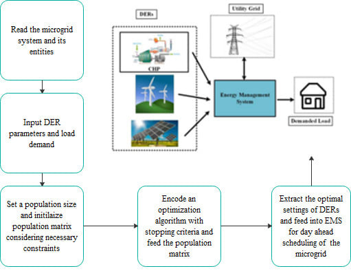
The following steps are the guidelines to implement the four algorithms for solving the concerned residential microgrid problem:

Step 1: For T hours of optimal scheduling, D numbers of DERs and N particles of the population, initialize the population matrix as stated in Equation (27). Each particle of the population consists of D DERs for T hours of scheduling. Hence, the size of every particle is (D*T), which is also the dimension of the problem. It is to be noted that every particle of the population must abide by the constraints mentioned in Equations (2)–(14).

$$S=\left[\begin{array}{l}{S}_{1,DER1}^1,S_{1,DER1}^2,\dots S_{1,DER1}^T,S_{1,DER2}^1,S_{1,DER2}^2,\dots S_{1,DER2}^T\dots S_{1,DERD}^1,S_{1,DERD}^2,\dots S_{1,DERD}^T\\ S_{2,DER1}^1,S_{2,DER1}^2,\dots S_{2,DER1}^T,S_{2,DER2}^1,S_{2,DER2}^2,\dots S_{2,DER2}^T\dots S_{2,DERD}^1,S_{2,DERD}^2,\dots S_{2,DERD}^T\\ S_{3,DER1}^1,S_{3,DER1}^2,\dots S_{3,DER1}^T,S_{3,DER2}^1,S_{3,DER2}^2,\dots S_{3,DER2}^T\dots S_{3,DERD}^1,S_{3,DERD}^2,\dots S_{3,DERD}^T\\ \dots \dots \dots \dots .\\ \dots \dots \dots \dots .\\ S_{N,DER1}^1,S_{N,DER1}^2,\dots S_{N,DER1}^T,S_{N,DER2}^1,S_{N,DER2}^2,\dots S_{N,DER2}^T\dots S_{N,DERD}^1,S_{N,DERD}^2,\dots S_{N,DERD}^T\end{array}\right],$$

(27)

Numerous initial solution sets are generated depending upon the population size N. Each particle of the population matrix S represents the position of different search agents (grey wolves) and is a potential and reasonable solution set (control variables).

Step 2: Calculate the fitness function for every particle of the population. Each fitness value represents the distance of the individual wolf from the prey.

Step 3: Initialize the parameters a, A, and C using Equation (19).

Step 4: Sort the population from best to worst. The best, second best, third best, and fourth best particles of the population are ranked as X_α, X_β, X_δ, and X_Ω. Since it is a minimization problem, the position of a search agent with least value of fitness function is the best position among all the search agents and is termed as X_α. The rest of the position is termed gradually as mentioned.

Step 5: Evaluate the parameters D_α, D_β, D_δ, and D_Ω using Equations (16), (21), or (24) as per the choice of the algorithm.

Step 6: Update the position of the particles using Equations (17) and (18) or (22) and (23) as per the choice of the algorithm.

Step 7: Check if all the particles abide by the constraints listed in Equations (2)–(14).

Step 8: Go to Step 2 until the maximum number of iterations is reached.

4. Results and Discussions

4.1. System Description

A LV utility connected microgrid system has been considered in this paper, both dispatchable and non-dispatchable distributed generators supply power to the system. Dispatchable generators include the conventional fossil-fueled generators, whereas the non-dispatchable generators denote the renewable energy sources whose power output cannot be controlled or scheduled. The aim is to optimally schedule the dispatchable generators using the proposed Modified Grey Wolf Optimization-Sine Cosine Algorithm-Crow Search Algorithm (MGWOSCACSA) algorithm. Two strategies (S1 and S2) and three cases (C0, C1, and C2) per strategy were studied for optimally scheduling the DGs of the test system. The description of the strategies and cases are displayed in

Table 1. Description of strategies.

Parameters	Strategy 1	Strategy 2
Fixed loads	Yes	Yes
Adjustable variable loads	No	Yes
Maintaining up/down time	No	Yes

and

Table 2. Description of Cases.

Cases	Description
C0	No Grid support
C1	Passive Grid support means grid can only sell power
C2	Active Grid support means grid can both buy and sell power

, respectively. Variable loads are those types of loads that consume power only for a particular period of the day: Water pump, air conditioners, and TVs fall in the category of variable loads. The characteristic features of the dispatchable generators are shown in

Table 3. Generator features [24].

DG Unit	Price Bids ($/kWh)	Operating Range (kW)	Min Up/Down Time (h)
G1	27.7	1/5	3
G2	39.1	1/5	3
G3	61.1	0.8/3	1
G4	65.6	0.8/3	1

. The power output from non-dispatchable (ND) generators, including the amount of fixed load (FL), is shown in Figure 2.

The features of the variable loads are displayed in

Table 4. Features of adjustable loads [24].

Load	Operating Range (kW)	Total Energy (kWh)	Operating Time (h)	Min Up Time (h)
L1	0/0.4	1.6	11–15	1
L2	0/0.4	1.6	15–19	1
L3	0.02/0.8	2.4	16–18	1
L4	0.02/0.8	2.4	14–22	1
L5	1.8/2	47	1–24	24

. Figure 3 shows the electricity market price. A battery is connected to the system with a maximum charging/discharging power of +4/−4 kW. The battery can charge or discharge for a maximum of six hours at a stretch. The algorithms GWO, Modified Grey Wolf Optimization-Crow Search Algorithm (MGWOCSA), Modified Grey Wolf Optimization-Sine Cosine Algorithm (MGWOSCA), and MGWOSCACSA are implemented to reduce the generation cost of the microgrid system operating in all six modes. To carry on an unbiased comparative analysis, all of these algorithms are executed with a population size of 80 and for 1000 iterations. The value of ‘fl’ for MGWOCSA and proposed MGWOSCACSA is fixed at 2.

4.2. Analysis of Results Obtained

After executing each of the four algorithms for 30 experiments, the generation cost of the microgrid system and their statistical characteristics are displayed in

Table 5. Statistical records of fitness function evaluated using various optimization techniques.

Algorithm	Best	Worst	Average	SD
	($)	($)	($)
S1C0
GWO	9953.1365	10,005.1523	9956.6042	13.20
MGWOSCA	9942.5534	9962.5412	9943.8859	5.07
MGWOCSA	9945.1286	9951.2356	9945.3322	1.11
MGWOSCACSA	9936.9188	9939.1254	9936.9924	0.40
S1C1
GWO	9315.007	9321.1528	9316.2362	2.50
MGWOSCA	9210.1591	9211.7845	9210.3758	0.56
MGWOCSA	9222.411	9232.1247	9223.7062	3.36
MGWOSCACSA	9208.4772	9209.2351	9208.5025	0.14
S1C2
GWO	8325.6346	8330.2212	8326.7048	1.97
MGWOSCA	8256.7778	8266.7812	8258.4450	3.79
MGWOCSA	8319.8155	8321.1095	8319.9880	0.45
MGWOSCACSA	8246.6734	8246.9885	8246.7049	0.10
S2C0
GWO	13,798.7739	13,802.2023	13,799.3453	1.30
MGWOSCA	13,763.2827	13,763.5023	13,763.2900	0.04
MGWOCSA	13,763.5064	13,763.9457	13,763.5210	0.08
MGWOSCACSA	13,763.2430	13,763.2605	13,763.2436	0.003
S2C1
GWO	12,761.2474	12,781.4577	12,766.3000	8.91
MGWOSCA	12,571.8116	12,573.4125	12,571.9183	0.41
MGWOCSA	12,566.7490	12,569.7714	12,567.2527	1.15
MGWOSCACSA	12,565.8610	12,566.9119	12,565.8960	0.19
S2C2
GWO	12,703.2581	12,710.3524	12,704.2040	2.45
MGWOSCA	12,502.0434	12,507.4524	12,502.5843	1.65
MGWOCSA	12,470.1601	12,473.5511	12,470.3862	0.86
MGWOSCACSA	12,460.9970	12,462.2785	12,461.0824	0.33

S = Strategy; C = Case, Bold indicates best-attained value.

. The four basic inferences obtained from the results are:

i.

The generation costs of strategy 1 are lower than those of strategy 2. This is because of the inclusion of the high-end variable loads in the second strategy.

ii.

The generation costs are C0 > C1 > C2. This is due to the active participation of the grid in Case 2 compared to its absence in Case 0 and partial participation in Case 1. The positive impact of an actively participating grid in a microgrid system can be realised from the difference in generation cost of C0 and C2 for both the strategies. For S1, there was a 17% savings in generation cost between C0 and C2. For S2, there was a 9% savings in generation cost between C0 and C2.

iii.

The total fixed load of the microgrid system is 290.5 kW, and the generation cost to satisfy the load demand was $8246. The average cost of electricity in this case was 28.38 $/kW. However, when the residential loads were considered, an additional 55 kW load was introduced in the LV microgrid system, which raised the load demand to 345.5 kW. The generation cost in this case was $12,460. The average cost of electricity for this case was 36.06 $/kW. A 19% rise in load demand incurred a 55% rise in the generation cost of the microgrid system.

iv.

MGWOSCACSA has been consistently delivering better accuracy results with superior statistical parameters for all the strategies and cases studied. This, in a way, claims the robustness and effectiveness of the proposed approach.

For Case 0, i.e., when the microgrid system is operating in islanded mode, Figure 4 shows the UP of the DERs for S1C0 and S2C0 modes of operation. It can be realized from Figure 4 that the UP of the DERs varies as G1 > G2 > G3 > G4. This pattern is due to the effect of the price bid of DERs as highlighted in Table 3. The higher the cost coefficient of the DER, the lesser the DER is utilized. If all the DERs were utilized for 24 h, the demand during S2C0 would have been met at the cost of $17,152. The optimization tool utilizes only the least priced DERs to their maximum possible limit, and the cost is minimized to $13,763, saving 19%. It can be seen that DERs G1 and G2 almost input 100% of their total strength throughout the day to fulfil the load demand. This is impractical and unreliable. If either G1 or G2 fails, there would be a surging rise in the generation cost or there is a high probability of system blackout. This is where C1 and C2 come into consideration. These two cases involve the participation of the grid, thereby assisting the DERs to operate within a long-lasting and relaxing limit. Further S2, along with increasing load demands by involving adjustable loads, also introduces the start-up/shut down time for the DERs, which is necessary for their maintenance and increasing their longevity.

Figure 5, Figure 6, Figure 7 and Figure 8 show the convergence curve characteristics of the algorithms implemented to minimize the generation cost of the system for various strategies and cases. MGWOSCACSA is consistent in providing the least possible generation cost compared to the rest of the algorithms.

Figure 9 is the pictorial representation of the best costs by the algorithms from Table 5. The rise of the generation costs for all cases of Strategy 2 is due to the involvement of the adjustable loads of the residential microgrid.

Figure 10 shows the hourly costs by the algorithms for strategy 1. The numbers 0, 1, and 2 along the name of the algorithms in the legend denote cases. The lowest of the generation costs is often attained in Case 2. This is due to the active participation of the grid in buying and selling power. Additionally, the proposed MGWOSCACSA algorithm yielded the lowest hourly costs for all the cases.

Figure 11 shows the contribution of the grid for the mentioned cases. Figure 11 shows that for the same period of the day, less power was bought by grid during S2C2 compared to that of S1C2. This is solely due to the raise in load demand during S2C2 by the inclusion of residential loads.

Figure 12 presents the complementary behaviour between the powers bought or sold by the grid and the electricity market price. When the market price of electricity is high, the grid sells power and vice versa. It is because of this transaction mechanism of the grid that the generation cost in case C2 is always less than C0 and C1.

The distribution of the adjustable loads when the minimum cost was obtained using MGWOSCACSA is shown in Figure 13. It can be observed that the adjustable loads (L1-L5) follow all the necessary constraints assigned.

Figure 14 and Figure 15 show the hourly output of the generators for case S1C2 and S2C2, respectively. The generators deliver power throughout the day according to Figure 14, whereas in Figure 15 the generators do not operate for some hours in the beginning and end of the day, thereby maintaining their minimum up/down time.

Figure 16 shows the charging and discharging states of the battery for the mentioned cases. As desired, for both the strategies, the battery did not charge/discharge for more than 6 h and maintained its maximum charging and discharging power of +4/−4 kW, respectively.

UP for all the DERs are shown in Figure 17. The DERs with the highest cost-coefficients are utilized less to meet the load demands.

4.3. Statistical Analysis and Solution Quality Check

To validate the efficiency and robustness of the proposed MGWOSCACSA, a meticulous analysis of the results obtained was performed by executing all the five algorithms for 30 times for both the test systems. Box plots are shown in Figure 18, which is drawn utilizing the mean values and standard deviation of the generation cost obtained by the algorithms after 30 trials for S2C2. A statistical analysis called Wilcoxon’s signed-rank test was also performed to prove the efficacy of the algorithms [42]. Let H₀ be a hypothesis that states that there is not any difference between the five methods, and H₁ be the alternative hypothesis stating that the ways are different. The significance level, α, is chosen as 0.05.

Table 6. Wilcoxon’s Rank Test on various values obtained using MGWOSCACSA.

Strategy	Best Cost	Worst Cost	Average	SD	p-Value (*10−7)
	($)	($)	($)
S1C0	9936.9188	9939.1254	9936.9924	0.40	0.6799
S1C1	9208.4772	9209.2351	9208.5025	0.14	0.6799
S1C2	8246.6734	8246.9885	8246.7049	0.10	1.4403
S2C0	13,763.2430	13,763.260	13,763.2436	0.003	0.6799
S2C1	12,565.8610	12,566.911	12,565.8960	0.19	0.6799
S2C2	12,460.9970	12,462.278	12,461.0824	0.33	1.0135

* means that the values of the entire column are multiplied with 10⁻⁷.

shows the best, worst, and mean value of the objective function along with the standard deviation for all the test systems using MGWOSCACSA. ‘p-value’ less than 0.05 for all the test systems contradicts the null hypothesis and proves the Wilcoxon’s signed rank test true for the proposed algorithm.

Figure 19 shows the average computational time of 30 trials and 1000 iterations/trial for all the algorithms used to minimize the generation cost for both the strategies in grid-connected modes. It is clearly seen that for all the strategies proposed, MGWOSCACSA consumed the least amount of computational time compared to GWO and its other hybrids.

5. Conclusions

This paper concentrated on diminishing the generation cost of an LV grid-connected residential microgrid system supported by RES and energy storage device. The major findings are listed below:

• A 50% inflation in the microgrid generation cost was realised when the residential loads, and they were taken into consideration. This rise in generation cost is huge and unavoidable but can be controlled if the home appliances were used sensibly. The operation of conventional fossil fuelled generators releases harmful toxic gases in the atmosphere. It is to be noted that less and sensible use of home appliances, e.g., AC and water pump, etc., will not only reduce the generation cost of the system but also minimize the usage of the conventional fossil-fuelled generators.
• The impact of active participation of grid in lowering the generation cost of the microgrid system can be seen from cases C0 and C2 for both the strategies. When compared to the generation cost of C0, 9–17% savings in the generation cost were incurred for case C2 during both the strategies of microgrid operation. The fact that the grid can both buy and sell power to and from the microgrid system contributes to the savings in C2 when compared to C0.
• To minimize the microgrid generation cost, hybrid MGWOSCACSA provides better and prominent solutions, employing the minimum computational time. Various statistical analysis also ranked the proposed algorithm as the best among the four. The results presented a good accuracy. Owing to its notable features of handling large dimensional objective functions, less computational time and high robustness MGWOSCACSA can be implemented to solve many other power system optimization problems.

As a scope of future research on this work, the emission coefficients of the non-conventional generators can be considered, and the optimization could be done to minimize the emission of harmful pollutants in the atmosphere. Furthermore, a multi-objective approach could be implemented to find a compromised solution with reduced generation cost and harmful pollutants.

References

- Yalcinoz, T.; Short, M. Neural networks approach for solving economic dispatch problem with transmission capacity constraints. IEEE Trans. Power Syst. 1998, 13, 307–313. [Google Scholar] [CrossRef]
- Wang, C.; Shahidehpour, S. Ramp-rate limits in unit commitment and economic dispatch incorporating rotor fatigue effect. IEEE Trans. Power Syst. 1994, 9, 1539–1545. [Google Scholar] [CrossRef]
- Dhillon, J.; Parti, S.; Kothari, D. Stochastic economic emission load dispatch. Electr. Power Syst. Res. 1993, 26, 179–186. [Google Scholar] [CrossRef]
- Chen, C.; Duan, S.; Cai, T.; Liu, B.; Hu, G. Smart energy management system for optimal microgrid economic operation. IET Renew. Power Gener. 2011, 5, 258–267. [Google Scholar] [CrossRef]
- Jiang, Q.; Xue, M.; Geng, G. Energy management of microgrid in grid-connected and stand-alone modes. IEEE Trans. Power Syst. 2013, 28, 3380–3389. [Google Scholar] [CrossRef]
- Wibowo, R.S.; Firmansyah, K.R.; Aryani, N.K.; Soeprijanto, A. Dynamic economic dispatch of hybrid microgrid with energy storage using quadratic programming. In Proceedings of the 2016 IEEE Region 10 Conference (TENCON), Singapore, 22–25 November 2016; pp. 667–670. [Google Scholar]
- Askarzadeh, A. A memory-based genetic algorithm for optimization of power generation in a microgrid. IEEE Trans. Sustain. Energy 2017, 9, 1081–1089. [Google Scholar] [CrossRef]
- Gholami, K.; Dehnavi, E. A modified particle swarm optimization algorithm for scheduling renewable generation in a micro-grid under load uncertainty. Appl. Soft Comput. 2019, 78, 496–514. [Google Scholar] [CrossRef]
- Ramli, M.A.; Bouchekara, H.; Alghamdi, A.S. Efficient energy management in a microgrid with intermittent renewable energy and storage sources. Sustainability 2019, 11, 3839. [Google Scholar] [CrossRef] [Green Version]
- Lahon, R.; Gupta, C.P.; Fernandez, E. Priority-Based Scheduling of Energy Exchanges Between Cooperative Microgrids in Risk-Averse Environment. IEEE Syst. J. 2019, 14, 1098–1108. [Google Scholar] [CrossRef]
- Lahon, R.; Gupta, C.P. Risk-based coalition of cooperative microgrids in electricity market environment. IET Gener. Transm. Distrib. 2018, 12, 3230–3241. [Google Scholar] [CrossRef]
- Lahon, R.; Gupta, C.P.; Fernandez, E. Optimal power scheduling of cooperative microgrids in electricity market environment. IEEE Trans. Ind. Inform. 2018, 15, 4152–4163. [Google Scholar] [CrossRef]
- Lahon, R.; Gupta, C.P. Energy management of cooperative microgrids with high-penetration renewables. IET Renew. Power Gener. 2017, 12, 680–690. [Google Scholar] [CrossRef]
- Dey, B.; Sharma, S. Energy Management of Microgrids with Renewables using soft computing techniques. In Proceedings of the 2015 Annual IEEE India Conference (INDICON), New Delhi, India, 17–20 December 2015; pp. 1–6. [Google Scholar]
- Dey, B.; Bhattacharyya, B.; Sharma, S. Optimal Sizing of Distributed Energy Resources in a Microgrid System with Highly Penetrated Renewables. Iran. J. Sci. Technol. Trans. Electr. Eng. 2019, 43, 527–540. [Google Scholar] [CrossRef]
- Dey, B.; Bhattacharyya, B.; Sharma, S. Robust economic dispatch of microgrid with highly penetrated renewables and energy storage system. Int. J. Energy Optim. Eng. 2019, 8, 67–87. [Google Scholar] [CrossRef]
- Trivedi, I.N.; Jangir, P.; Bhoye, M.; Jangir, N. An economic load dispatch and multiple environmental dispatch problem solution with microgrids using interior search algorithm. Neural Comput. Appl. 2018, 30, 2173–2189. [Google Scholar] [CrossRef]
- Elattar, E.E. Modified harmony search algorithm for combined economic emission dispatch of microgrid incorporating renewable sources. Energy 2018, 159, 496–507. [Google Scholar] [CrossRef]
- Dey, B.; Roy, S.K.; Bhattacharyya, B. Solving multi-objective economic emission dispatch of a renewable integrated microgrid using latest bio-inspired algorithms. Eng. Sci. Technol. Int. J. 2019, 22, 55–66. [Google Scholar] [CrossRef]
- Bahmani-Firouzi, B.; Azizipanah-Abarghooee, R. Optimal sizing of battery energy storage for micro-grid operation management using a new improved bat algorithm. Int. J. Electr. Power Energy Syst. 2014, 56, 42–54. [Google Scholar] [CrossRef]
- Sharma, S.; Bhattacharjee, S.; Bhattacharya, A. Operation cost minimization of a micro-grid using quasi-oppositional swine influenza model based optimization with quarantine. Ain Shams Eng. J. 2018, 9, 45–63. [Google Scholar] [CrossRef] [Green Version]
- Sharma, S.; Bhattacharjee, S.; Bhattacharya, A. Grey wolf optimisation for optimal sizing of battery energy storage device to minimise operation cost of microgrid. IET Gener. Transm. Distrib. 2016, 10, 625–637. [Google Scholar] [CrossRef]
- Sharma, S.; Bhattacharjee, S.; Bhattacharya, A. Probabilistic operation cost minimization of Micro-Grid. Energy 2018, 148, 1116–1139. [Google Scholar] [CrossRef]
- Khodaei, A. Provisional microgrids. IEEE Trans. Smart Grid 2014, 6, 1107–1115. [Google Scholar] [CrossRef]
- Khodaei, A. Provisional microgrid planning. IEEE Trans. Smart Grid 2015, 8, 1096–1104. [Google Scholar] [CrossRef]
- Dey, B.; Bhattacharyya, B. Dynamic cost analysis of a grid connected microgrid using neighborhood based differential evolution technique. Int. Trans. Electr. Energy Syst. 2019, 29, e2665. [Google Scholar] [CrossRef] [Green Version]
- Kumar, K.P.; Saravanan, B. Day ahead scheduling of generation and storage in a microgrid considering demand Side management. J. Energy Storage 2019, 21, 78–86. [Google Scholar] [CrossRef]
- Koltsaklis, N.E.; Giannakakis, M.; Georgiadis, M.C. Optimal energy planning and scheduling of microgrids. Chem. Eng. Res. Des. 2018, 131, 318–332. [Google Scholar] [CrossRef]
- Albaker, A.; Majzoobi, A.; Zhao, G.; Zhang, J.; Khodaei, A. Privacy-preserving optimal scheduling of integrated microgrids. Electr. Power Syst. Res. 2018, 163, 164–173. [Google Scholar] [CrossRef]
- Talapur, G.G.; Suryawanshi, H.M.; Xu, L.; Shitole, A.B. A reliable microgrid with seamless transition between grid connected and islanded mode for residential community with enhanced power quality. IEEE Trans. Ind. Appl. 2018, 54, 5246–5255. [Google Scholar] [CrossRef] [Green Version]
- Li, S.; Yang, J.; Fang, J.; Liu, Z.; Zhang, H. Electricity scheduling optimisation based on energy cloud for residential microgrids. IET Renew. Power Gener. 2019, 13, 1105–1114. [Google Scholar] [CrossRef]
- Liu, W.; Liu, C.; Lin, Y.; Bai, K.; Ma, L. Interval multi-objective optimal scheduling for redundant residential microgrid with VESS. IEEE Access 2019, 7, 87849–87865. [Google Scholar] [CrossRef]
- Sattarpour, T.; Golshannavaz, S.; Nazarpour, D.; Siano, P. A multi-stage linearized interactive operation model of smart distribution grid with residential microgrids. Int. J. Electr. Power Energy Syst. 2019, 108, 456–471. [Google Scholar] [CrossRef]
- Wen, L.; Zhou, K.; Yang, S.; Lu, X. Optimal load dispatch of community microgrid with deep learning based solar power and load forecasting. Energy 2019, 171, 1053–1065. [Google Scholar] [CrossRef]
- Gu, W.; Lu, S.; Wu, Z.; Zhang, X.; Zhou, J.; Zhao, B.; Wang, J. Residential CCHP microgrid with load aggregator: Operation mode, pricing strategy, and optimal dispatch. Appl. Energy 2017, 205, 173–186. [Google Scholar] [CrossRef]
- Mohseni, A.; Mortazavi, S.S.; Ghasemi, A.; Nahavandi, A. The application of household appliances’ flexibility by set of sequential uninterruptible energy phases model in the day-ahead planning of a residential microgrid. Energy 2017, 139, 315–328. [Google Scholar] [CrossRef]
- Anvari-Moghaddam, A.; Monsef, H.; Rahimi-Kian, A. Optimal smart home energy management considering energy saving and a comfortable lifestyle. IEEE Trans. Smart Grid 2014, 6, 324–332. [Google Scholar] [CrossRef]
- Mirjalili, S.; Mirjalili, S.M.; Lewis, A. Grey wolf optimizer. Adv. Eng. Softw. 2014, 69, 46–61. [Google Scholar] [CrossRef] [Green Version]
- Khandelwal, A.; Bhargava, A.; Sharma, A.; Sharma, H. Modified grey wolf optimization algorithm for transmission network expansion planning problem. Arab. J. Sci. Eng. 2018, 43, 2899–2908. [Google Scholar] [CrossRef]
- Mirjalili, S. SCA: A sine cosine algorithm for solving optimization problems. Knowl.-Based Syst. 2016, 96, 120–133. [Google Scholar] [CrossRef]
- Askarzadeh, A. A novel metaheuristic method for solving constrained engineering optimization problems: Crow search algorithm. Comput. Struct. 2016, 169, 1–12. [Google Scholar] [CrossRef]
- Woolson, R. Wilcoxon signed-rank test. In Wiley Encyclopedia of Clinical Trials; Wiley: Hoboken, NJ, USA, 2007; pp. 1–3. [Google Scholar]
Figure 1.
Pictorial description of a typical low voltage (LV) microgrid.
Figure 2.
Fixed loads and power outputs from non-dispatchable generators [24].
Figure 3.
Market price of electricity [24].
Figure 4.
UP of distributed energy resources (DERs) when minimum cost was obtained using Modified Grey Wolf Optimization-Sine Cosine Algorithm-Crow Search Algorithm (MGWOSCACSA) for Case 0.
Figure 5.
Convergence curves of algorithms for operation mode S1C1.
Figure 6.
Convergence curves of algorithms for operation mode S1C2.
Figure 7.
Convergence curves of algorithms for operation mode S2C1.
Figure 8.
Convergence curves of algorithms for operation mode S2C2.
Figure 9.
Cost comparative analysis amongst all strategies, cases, and algorithms used.
Figure 10.
Hourly costs by various algorithms during S1.
Figure 11.
Grid contribution when minimum cost was obtained using MGWOSCACSA.
Figure 12.
Grid output (kW) vs. Electricity price ($/kW).
Figure 13.
Distribution of adjustable loads when minimum cost was obtained using MGWOSCACSA for S2C2 operation mode.
Figure 14.
Hourly outputs of generators for S1C2 mode using MGWOSCACSA.
Figure 15.
Hourly outputs of generators for S2C2 mode using MGWOSCACSA.
Figure 16.
Battery outputs for various modes of operation using MGWOSCACSA.
Figure 17.
Utilization Percentage of the DERs for various strategies and cases.
Figure 18.
Box plots for all the algorithms during S2C2.
Figure 19.
Computational time.