Numerical Modeling of CO₂ Sequestration within a Five-Spot Well Pattern in the Morrow B Sandstone of the Farnsworth Hydrocarbon Field: Comparison of the TOUGHREACT, STOMP-EOR, and GEM Simulators

Abstract

The objectives of this study were (1) to assess the fate and impact of CO₂ injected into the Morrow B Sandstone in the Farnsworth Unit (FWU) through numerical non-isothermal reactive transport modeling, and (2) to compare the performance of three major reactive solute transport simulators, TOUGHREACT, STOMP-EOR, and GEM, under the same input conditions. The models were based on a quarter of a five-spot well pattern where CO₂ was injected on a water-alternating-gas schedule for the first 25 years of the 1000 year simulation. The reservoir pore fluid consisted of water with or without petroleum. The results of the models have numerous broad similarities, such as the pattern of reservoir cooling caused by the injected fluids, a large initial pH drop followed by gradual pH neutralization, the long-term persistence of an immiscible CO₂ gas phase, the continuous dissolution of calcite, very small decreases in porosity, and the increasing importance over time of carbonate mineral CO₂ sequestration. The models differed in their predicted fluid pressure evolutions; amounts of mineral precipitation and dissolution; and distribution of CO₂ among immiscible gas, petroleum, formation water, and carbonate minerals. The results of the study show the usefulness of numerical simulations in identifying broad patterns of behavior associated with CO₂ injection, but also point to significant uncertainties in the numerical values of many model output parameters.

1. Introduction

The Farnsworth Unit (FWU), a hydrocarbon field in northern Texas, USA, has been studied by the Southwest Regional Partnership on Carbon Sequestration (SWP) since 2013 as a test site for commercial-scale CO₂ sequestration and enhanced oil recovery (EOR) in a sandstone reservoir [1,2]. Central to assessing the feasibility of CO₂ sequestration in the FWU is determining the behavior of the injected CO₂, including where and at what rate the CO₂ will migrate, how the CO₂ will be distributed among the pore fluid phases (i.e., aqueous, gas, and nonaqueous liquid) and minerals, and how the hydraulic properties of the reservoir and the composition of the pore fluids will be changed.

Answering these questions requires the ability to quantify the flow of multiple fluid phases, their transport of solute and heat, and chemical reactions involving the fluid phases and minerals in the reservoir. Several previous SWP studies have attempted to do this using numerical reactive transport modeling. Ahmmed [3] used the TOUGHREACT software [4] to model reservoir behaviors caused by CO₂ injection in the immediate vicinity of an individual well and over the full area of the FWU. His model predicted the pH of the formation water to decline to a minimum of 4.7 because of CO₂ injection, causing most of the native minerals in the reservoir to dissolve, except for quartz, kaolinite, and illite. The model predicted hydrodynamic trapping to be the main mechanism of CO₂ sequestration, with ankerite predicted to be the only mineral that sequestered CO₂. The changes in mineral abundance, however, were predicted to be too small to cause much change in the hydraulic properties of the reservoir. Limitations of the model were that it did not include petroleum, only CO₂ was injected into the reservoir rather than water and CO₂ through a water alternating gas (WAG) scheme as actually implemented in the field, the model did not implement the actual regional pressure gradient occurring in the field, and the model was only carried out to 30 years.

Pan et al. [5] used the TOUGHREACT software to evaluate reactive transport in the Morrow B Sandstone resulting from WAG injection over a 5-spot well pattern. Because of the symmetry of the 5-spot well pattern, the model domain consisted of a triangle representing only one-eighth of the total 5-spot pattern area where the injection well and production well were separated by 504 m. Pan et al. [5] incorporated several chloride and sulfate minerals plus muscovite and dawsonite in their model as potential precipitates that were not incorporated in Ahmmed’s [3] model. However, except for halite, these minerals were not predicted to precipitate as described in the model by Pan et al. [5]. Besides the relatively small size of their model domain, limitations of the model constructed by Pan et al. [5] were that it did not treat petroleum and used mineral reactive surface areas per unit mass that are significantly larger than indicated by Gallagher’s [6] characterization of the Morrow B. Similar to Ahmmed et al. [3], Pan et al. [5] found the native reservoir minerals, quartz, kaolinite, and illite to increase in abundance over time, whereas the other native reservoir minerals dissolved. Like Ahmmed et al. [3], Pan et al. [5] found ankerite to be a mineral sink for injected CO₂, but also magnesite and siderite. Pan et al. [5] found their predicted changes in mineral abundances to cause only minor changes in the hydraulic properties of the reservoir—a maximum increase in porosity and permeability of 2.7 and 8.4%, respectively, occurring close to the injection well.

Khan [7] also used the TOUGHREACT software to model reactive transport in the Morrow B Sandstone as a result of WAG injection but considered a larger model domain than Pan et al. [5] consisting of the western part of the FWU. Like Ahmmed [3] and Pan et al. [5], Khan [7] considered water and CO₂ in his models but not petroleum. Khan’s [7] simulations predicted much of the injected CO₂ to leak from the reservoir into the overlying shales or to migrate across the western boundary of the FWU within a few decades. Khan’s [7] predicted mineral precipitation and dissolution behaviors resembled those of Ahmmed [3] and Pan et al. [5]. The native reservoir minerals, ankerite, albite, and illite were predicted to dissolve because of CO₂ injection but quartz; kaolinite; smectite; and the carbonate minerals calcite, dolomite, and siderite were predicted to precipitate. However, Khan’s [7] predicted porosity changes of order 0.001% were much smaller than those of Pan et al. [5].

Sun et al. [8] used the Computer Modeling Group Green House Gas (CMG-GHG) simulator, GEM [9,10], to model reactive transport of CO₂ injected through a WAG scheme over a model domain consisting of a 5-spot well pattern like that considered by Pan et al. [5]. The total simulation time in Sun et al. [8] was 1000 years, with injection occurring during the first 20 years. In contrast to Ahmmed [3], Pan et al. [5], and Khan [7], Sun et al. [8] predicted most of the injected CO₂ to be sequestered as an immiscible gas phase. Most of the remaining CO₂ in the model of Sun et al. [8] was sequestered through residual trapping. Like Ahmmed [3], Pan et al. [5], and Khan [7], Sun et al. [8] predicted the smallest amount of CO₂ sequestration to occur through mineral trapping. Sun et al. [8] predicted quartz, kaolinite, and siderite to precipitate in their simulations but albite, calcite, chlorite, dolomite, illite, and smectite to dissolve. Sun et al. [8] did not include ankerite or magnesite in their models, two potentially important mineral sinks for CO₂. Sun et al. [8] predicted porosity changes of less than 1% in their models.

White et al. [11] have developed a multi-fluid phase (water–oil–gas) reactive transport simulator called STOMP-EOR, which they applied to study the physical behavior of fluids in the western FWU. Like GEM, STOMP-EOR solves coupled conservation equations for energy, water mass, CO₂ mass, CH₄ mass, and the masses of multiple petroleum components in variably saturated geologic media. Although STOMP-EOR has the capability to compute reactive transport, STOMP-EOR had not yet been used in reactive transport modeling studies of the FWU.

Because the previous SWP investigations of the FWU used three different numerical simulators—TOUGHREACT, GEM, and STOMP-EOR, this raises the question of how consistent the simulators are in terms of their ability to model the same input conditions. Thus, one of the objectives of the present study was to try to answer this question by building identical five-spot pattern models with the same grid design and parameter values for all three simulators and comparing the results. Because TOUGHREACT currently does not have the capability to treat a separate petroleum fluid phase, the comparison of the TOUGHREACT, GEM, and STOMP-EOR models required that water and CO₂ were the only pore fluids. The TOUGHREACT simulator is analogous to the STOMP-CO₂ simulator, both considering only energy conservation, and conservation of water, CO₂, and salt mass. The equations of state differ significantly between STOMP-CO₂ and STOMP-EOR, with CO₂ properties being computed from the Span and Wager [12] equation of state, and cubic equations of state, respectively. A further comparison was made between GEM and STOMP-EOR for identical five-spot pattern models that included water, CO₂, and petroleum pore fluids.

In addition to providing a rigorous comparison of the TOUGHREACT, GEM, and STOMP-EOR simulators, the first of its kind and which will help build confidence in these simulators for future research, the present study also extends the previous reactive transport modeling studies of the FWU in the following ways:

• The studies by Ahmmed [3], Pan et al. [5], and Khan [7] considered only water and CO₂ as the pore fluids and not oil. The present study included a simulation scenario that considered water, CO₂, and oil.
• Although Sun et al. [8] considered water, CO₂, and oil in their reactive transport model, their model had some differences with actual field conditions: (1) They did not use the actual fluid injection temperature in the field, but rather the 75 °C temperature in the reservoir, and (2) they used generic mineral reactive surface areas from Pan et al. [5] and Xu et al. [13] rather than reactive surface areas determined from the field properties of the Morrow B. The present study used the field-based fluid injection temperatures and mineral reactive surface areas.

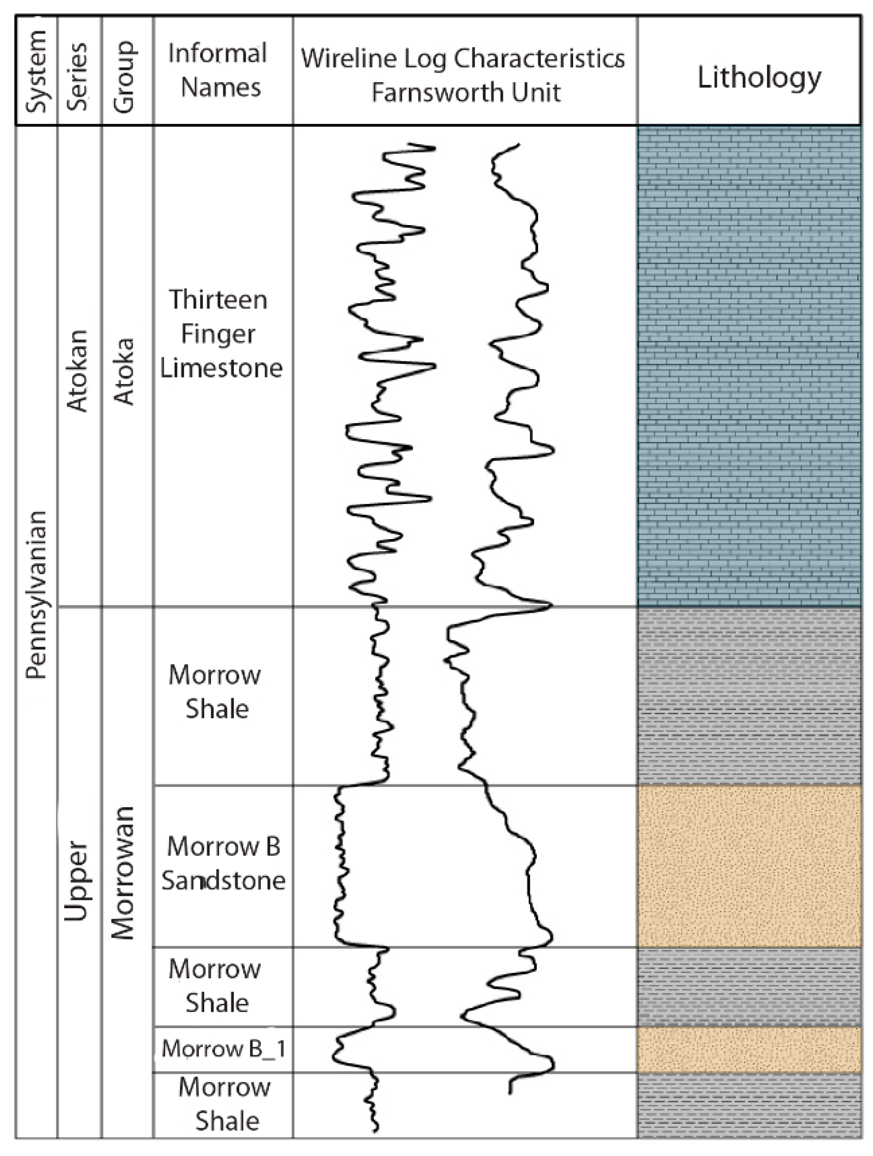
2. Geological Setting

The Farnsworth Unit is located in the western Anadarko Basin (Figure 1), a structural basin that formed primarily during the Mississippian and Pennsylvanian periods in response to the collision of southeastern North America with Gondwanaland. The Morrow B Sandstone, the main target for hydrocarbon production and CO₂ sequestration in the study, is part of the Upper Morrowan-age (Early Pennsylvanian) stratigraphic succession in the basin. This succession is characterized by alternating intervals of glacially induced marine transgression and regression. During times of marine transgression, increasingly fine-grained clastic sediments were deposited, culminating in the deposition of nearshore and offshore mud. During times of marine regression, streams flowed through the FWU from the northwest, carving channels through the older transgressive sediments. During subsequent marine transgression, the fluvial sediments deposited in these channels were winnowed to form coarse-grained lag deposits and then were buried by fine-grained clastic sediments. Thus, the Morrow B Sandstone consists of relatively narrow channels of coarse sandstone enclosed within fine-grained sediments, creating conditions favorable for stratigraphic CO₂ trapping.

The Morrow B Sandstone is subarkosic, with quartz and albite as the main constituents. The remainder of the Morrow B is composed of minor amounts of chlorite; the carbonate minerals, calcite, siderite, and ankerite; and the clay minerals, smectite, illite, and kaolinite. The Morrow B ranges in thickness from 0 to 16.5 m within the Farnsworth Unit, with an average thickness of 10 m [6,14]. The permeability and porosity of the Morrow B are very heterogeneous, with average values of approximately 48.2 mD and 14.5%, respectively. The Morrow B is overlain by the Morrow Shale and an Atokan-age sequence of low-permeability evaporites and limestone called the Thirteen Finger Limestone (Figure 2; [6,14,15,16,17]). Together, the Morrow Shale and Thirteen Finger Limestone act as a caprock for the Morrow B Sandstone [14,15].

3. Model Construction and Scenarios

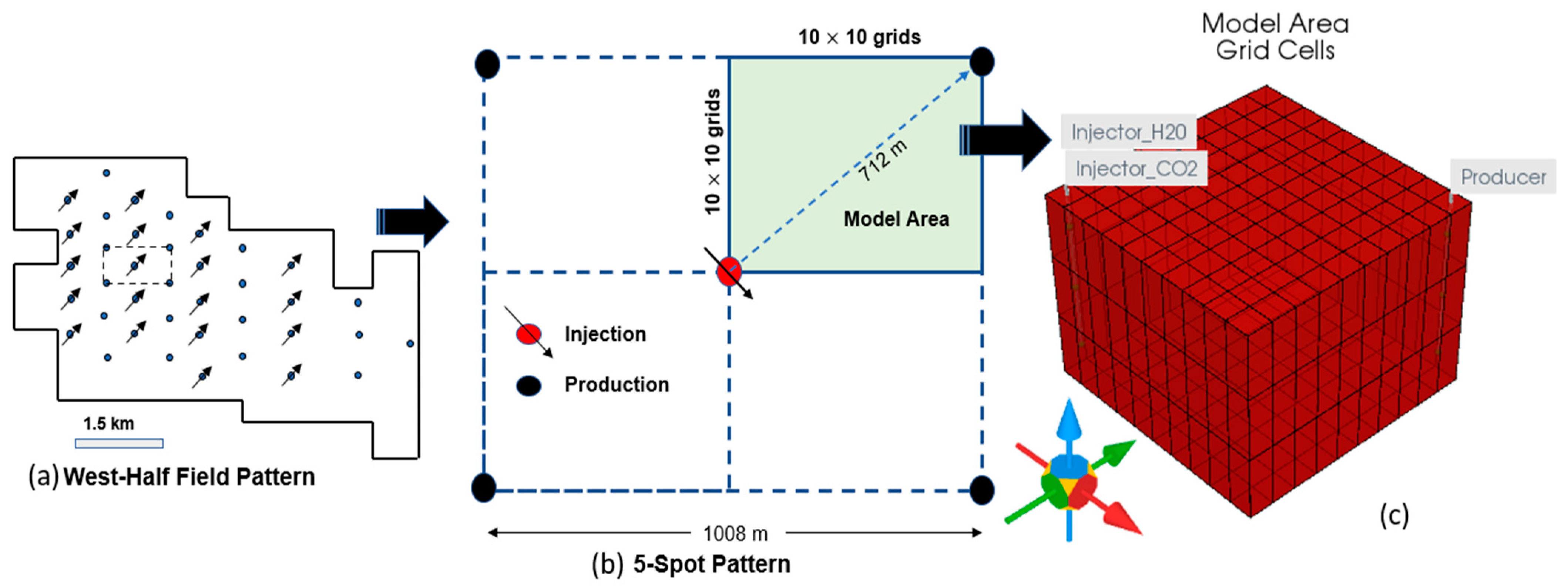
3.1. General Model Characteristics

The field development design within the Farnsworth Unit is a sequence of five-spot well patterns, in which four injection wells are placed at the corners of a square and a production well is placed at the center of the square. The numerical model generated in the present study is based on that five-spot well pattern, specifically on the pattern centered on production well, 13-10A, but because of the symmetry of the well spacing and in the expected model results, the model considers only one-quarter of the full pattern. Thus, the grid employed in the numerical model consisted of a three-dimensional block with an injection well at one corner and a production well at the opposite corner (Figure 3). The numerical grid had horizontal lengths of 504 m each subdivided by 11 equally spaced nodes, and a vertical length of 10 m, coinciding with the thickness of the Morrow B at well 13-10A, subdivided by 4 equally spaced nodes. The small model scale and spatial homogeneity of model parameters within the model domain were chosen to facilitate comparison of results from the three simulators.

All three numerical simulators solve mass and energy conservation equations for multi-phase pressure distribution and fluid flow, solute transport, and heat transport [18,19,20].

In TOUGHREACT and STOMP-EOR, these equations are solved using the integrated finite difference method. In GEM, these equations are solved using the finite difference method.

Hydrological parameter values used in the models were obtained from studies by Pan et al. [5] and are shown in

Table 1. Hydrogeologic parameters used in the STOMP-EOR, TOUGHREACT, and GEM simulations.

Matrix compressibility (1/Pa)	$4.5\times {10}^{-10}$
Diffusion coefficient (m2/s)
Gas Aqueous solutes	$1.1\times {10}^{-5}$ $2.1\times {10}^{-9}$
Rock matrix density (kg/m3)	$2500$
Porosity	$0.145$
Intrinsic Permeability
Horizontal (m2) Vertical Ratio	$4.74\times {10}^{-14}$ $0.10$
Relative Permeability (Corey, 1954 model)
Saturation endpoints Water/gas endpoints	${\mathrm{S}}_{\mathrm{l}\mathrm{r}}=0.3 \mathrm{a}\mathrm{n}\mathrm{d} {\mathrm{S}}_{\mathrm{g}\mathrm{r}}=1\times {10}^{-4}$ $\mathrm{K}\mathrm{r}\mathrm{w}=0.7 \mathrm{a}\mathrm{n}\mathrm{d} \mathrm{K}\mathrm{r}\mathrm{g}=1$
Capillary Pressure	None
Salt mass fraction in pore water	$0.003$
Initial aqueous phase saturation
Water–CO2 models Water–CO2–oil models	$0.99$ $0.73$
Initial gas-phase saturation	$0.01$
Initial oil-phase saturation (Water-CO2-oil models)	$0.27$
Initial field temperature (°C)	$75.56$
Injection pressure (MPa)	$34.47$
Injection temperature (°C)	$40$
Production well screen pressure (MPa)	$29.99$
WAG Cycle Ratio (Months)	$3:6$
Thermal conductivity of saturated rock (W/m K) Specific heat (J/kg K)	$2.28$ $700$

.

The initial Morrow B pore water composition used in the models was taken from Ahmmed et al. [21] and is shown in

Table 2. Concentrations of aqueous component species in the FWU reservoir from well battery AWT4.

Primary Aqueous Species (mol/L):
Ca2+	8.25 × 10−4	Ba2+	1.00 × 10−5
H+	1.00 × 10−7	${\mathrm{AlO}}_2^{-}$	2.80 × 10−7
K+	1.83 × 10−4	${\mathrm{SO}}_4^{2-}$	1.35 × 10−4
Mg2+	5.10 × 10−4	Cl−	5.90 × 10−2
Na+	6.18 × 10−2	${\mathrm{HCO}}_3^{-}$	1.33 × 10−2
Fe2+	3.60 × 10−13	SiO2	6.69 × 10−4

Data from Ahmmed et al. [21].

.

The minerals shown in

Table 3. Initial mineral volume fractions, possible secondary mineral phases, reactive surface areas, and kinetic properties at 25 °C.

Minerals	Initial Volume Fraction %	Reactive Surface Area cm2/g	Neutral pH Mechanism
			Rates Constant 25 °C [mol m−2 s−1]	Activation Energy [kJ mol−1]
Albite	17.973	11.45	$1.0\times {10}^{-12}$	67.83
Calcite	0.4279	11.07	$1.55\times {10}^{-7}$	23.50
Clinochlore	0.8559	11.41	$1.0\times {10}^{-13}$	62.76
Quartz	58.6261	9.80	$1.023\times {10}^{-14}$	87.70
Illite	0.5991	43.63	$1.7\times {10}^{-13}$	35.00
Kaolinite	7.018	46.15	$1.01\times {10}^{-13}$	62.76
Dolomite	0	10.49	$6.0\times {10}^{-10}$	41.80
Magnesite	0	10	$4.57\times {10}^{-10}$	23.50
Smectite-ca	0	9.8	$1.0\times {10}^{-14}$	58.62
Siderite	0	9.8	$1.26\times {10}^{-9}$	41.80
Ankerite	0	9.84	$1.26\times {10}^{-9}$	41.80

Mineral volume fraction data from Munson [14] and Gallagher [6].

include both the minerals that were initially present in the Morrow B (primary minerals) and new minerals that were expected possibly to precipitate during the model simulations (secondary minerals). The mineral reactive surface areas were obtained from Khan [7], which were calculated from the average radii of mineral grains in the Morrow B reported by Gallagher [6]. Kinetic parameters for mineral precipitation and dissolution were obtained from Palandri and Kharaka [22] and Xu et al. [19]. Mineral precipitation and dissolution reactions initially proceeded according to a neutral pH reaction mechanism because of the initially near-neutral pH of the Morrow B formation water. With the injection of CO₂, the formation water became progressively acidified and mineral precipitation and dissolution reactions then proceeded according to an acidic pH reaction mechanism. Chemical reactions that did not involve minerals were assumed to reach equilibrium within each time step, for example, the intra-aqueous species reactions.

All three numerical simulators use similar kinetic formulations [9,11,13], in which mineral dissolution and precipitation rates are calculated from

$$r_m={\widehat{A}}_m{k}_m\left(1-\frac{Q_m}{K_{eq, m}}\right)$$

(1)

where $r_m$ is the rate of dissolution or precipitation, ${\widehat{A}}_m$ is the reactive surface area of mineral m, $k_m$ is the rate constant, $K_{eq, m}$ is the chemical equilibrium constant, and Q_m is the activity product, expressed as

$$Q_m={\displaystyle \prod }_{k=1}^{n_{aq}}{a}_k^{v_{k_m}}$$

(2)

where $n_{aq}$ is the number of aqueous components, $v_{km}$ is the stoichiometric coefficient of component k in reaction m, and a_k is the activity of the component k.

Reaction rate constants at a temperature of interest are computed from

$$k_m=k_{25} exp\left[-\frac{E_a}{R}\left(\frac{1}{T}-\frac{1}{T_0}\right)\right]$$

(3)

where $E_a$ is the activation energy and $k_{25}$ is the reaction rate constant at 25 °C.

Other initial conditions are that the model domain had a constant pressure of 30 MPa and a constant temperature of 75 °C.

The boundary conditions for the models constructed for each simulator were the same. All the faces of the model domains had zero fluid flux boundary conditions. The lateral faces of the model domains had zero heat flux boundary conditions. A vertical injection well was placed at one corner of the model domain, and a production well was placed at the opposite corner (Figure 3). The wells were screened over an elevation from 0.0 m to 10.0 m. A WAG scheme was employed at the injection well in which water was injected at a rate of 0.336 kg/s at 40 °C for 90 days, after which CO₂ was injected at a rate of 0.454 kg/s for 180 days at 40 °C. This WAG scheme was employed for the first 25 years of each simulation, after which injection ceased and the simulation was allowed to continue to run to a total time of 1000 years to be able to track long-term effects of CO₂ injection. A constant bottom hole pressure of 30.0 MPa was assigned to the production well. The production and injection rates represent ¼ of the average pumping rates in the field from wells 13-9 and 8-4, as the model domains intersect only one-quarter of the perimeter of the wells.

During execution of the model, time step sizes were continuously and automatically adjusted to achieve convergence. In general, time step sizes increased with time as gradients in model parameters diminished.

3.2. Model Scenario 1: Injection of CO₂ into a Saline Water Aquifer

Pore fluids in the Morrow B Sandstone consist of water, petroleum, and methane. Thus, to model as robustly as possible the behavior of CO₂ injected into the Morrow B and to assess the CO₂ sequestration capacity of the Morrow B, all three pore fluids should be treated. This in fact was the objective of the present study’s second model scenario described below. However, another objective of the present study was to assess the consistency of major reactive solute transport simulators with one another for CO₂ sequestration modeling, specifically, the GEM, STOMP-EOR, and TOUGHREACT simulators. The TOUGHREACT simulator did not currently have the capacity to treat petroleum as a separate pore fluid. Thus, to the compare the performance of TOUGHREACT to the GEM and STOMP-EOR simulators, a scenario was chosen involving injection of CO₂ into the Morrow B where water was the only pore fluid present. This scenario has further value in that it provides a baseline for comparison. As noted above, the same parameter values (Table 1, Table 2 and Table 3), boundary conditions, and initial conditions were used with all three simulators to model this scenario.

3.3. Model Scenario 2: Injection of CO₂ into a Depleted Hydrocarbon Reservoir

This scenario investigates the effects of the coexistence of petroleum and water on CO₂ sequestration in the Morrow B Sandstone. The parameter values, boundary conditions, and initial conditions were the same as in Model scenario 1, except that the initial water saturation was reduced from 99% to 73% and oil saturation was raised from 0 to 16%. The initial gas saturation remained the same as in Model scenario 1 at 1%.

The composition of the petroleum used in the models is shown in

Table 4. Model petroleum component properties and initial mole fractions.

Component	Mole Fraction	Molar Weight (kg/kmol)	Critical Temperature (K)	Critical Pressure (bar)
CO2	0.0	44.01	304.21	73.77
CH4	0.385	16.04	188.85	46.00
C2	0.039	30.07	197.45	48.83
C3	0.025	44.10	247.19	42.44
C4+	0.028	58.12	289.89	37.76
C5+	0.020	72.15	328.13	33.76
C6	0.018	86.18	365.70	29.68
HC1	0.335	189.95	577.54	22.48
HC2	0.150	545.65	864.34	16.25

Component definitions, properties, and abundances derived from Sun et al. [8].

and is based on the FWU petroleum composition reported by Gunda et al. [23]. The presence of petroleum with water in a porous medium can significantly alter the sequestration behavior of CO₂ compared to the case when only water is initially present in the porous medium. A significant fraction of the injected CO₂ is expected to dissolve into the petroleum, leaving less CO₂ to exist as a separate immiscible gas phase and to dissolve into the formation water, affecting the physical flow behavior of the pore fluids through altered relative permeability values. Lower CO₂ concentration in the formation water will raise its pH, fundamentally affecting the concentrations of other aqueous species and the precipitation and dissolution of minerals. As noted above, only GEM and STOMP-EOR were used to investigate Model scenario 2, as TOUGHREACT did not currently have the capability to treat a separate petroleum fluid phase.

4. Results

4.1. Model Scenario 1

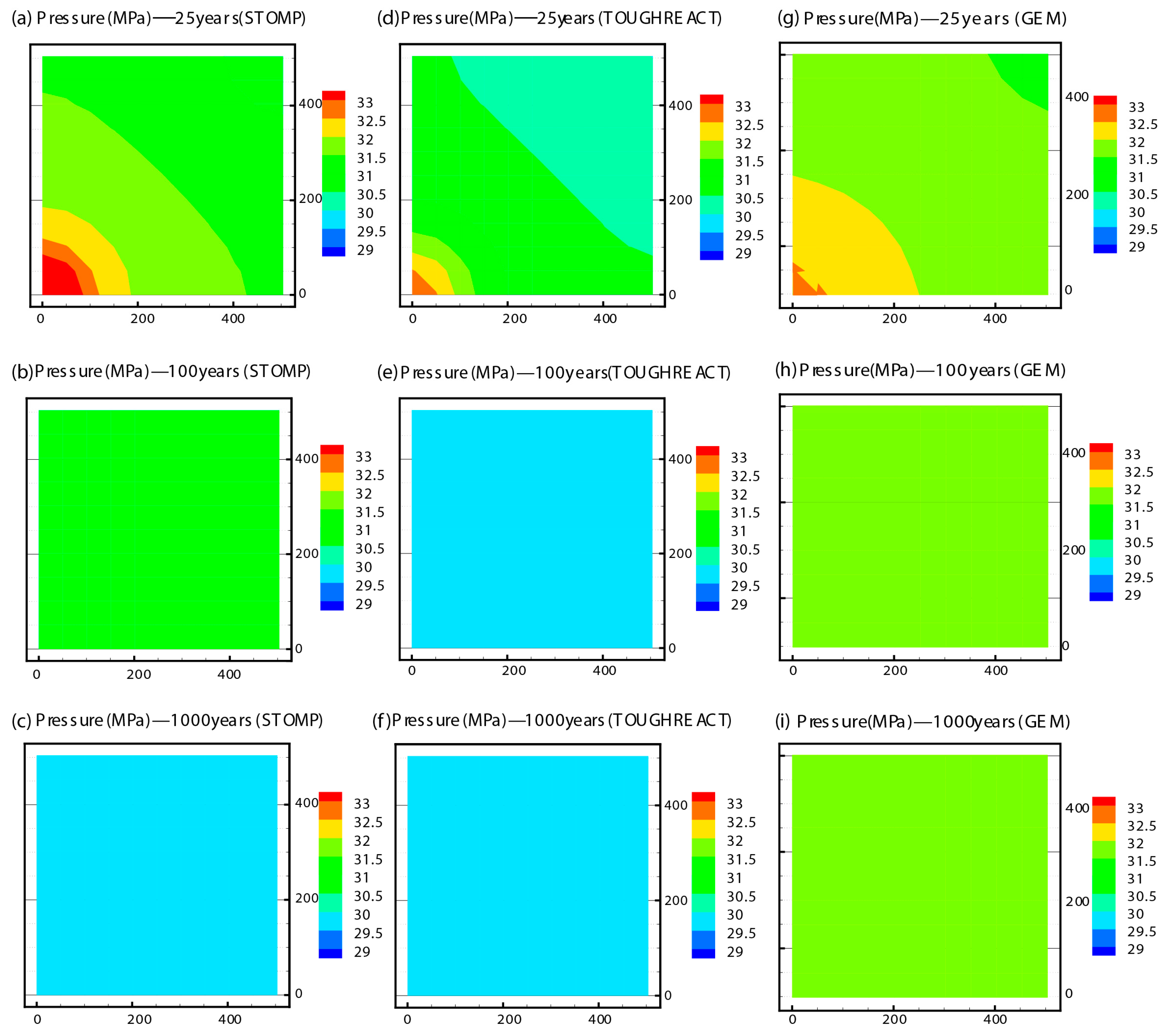
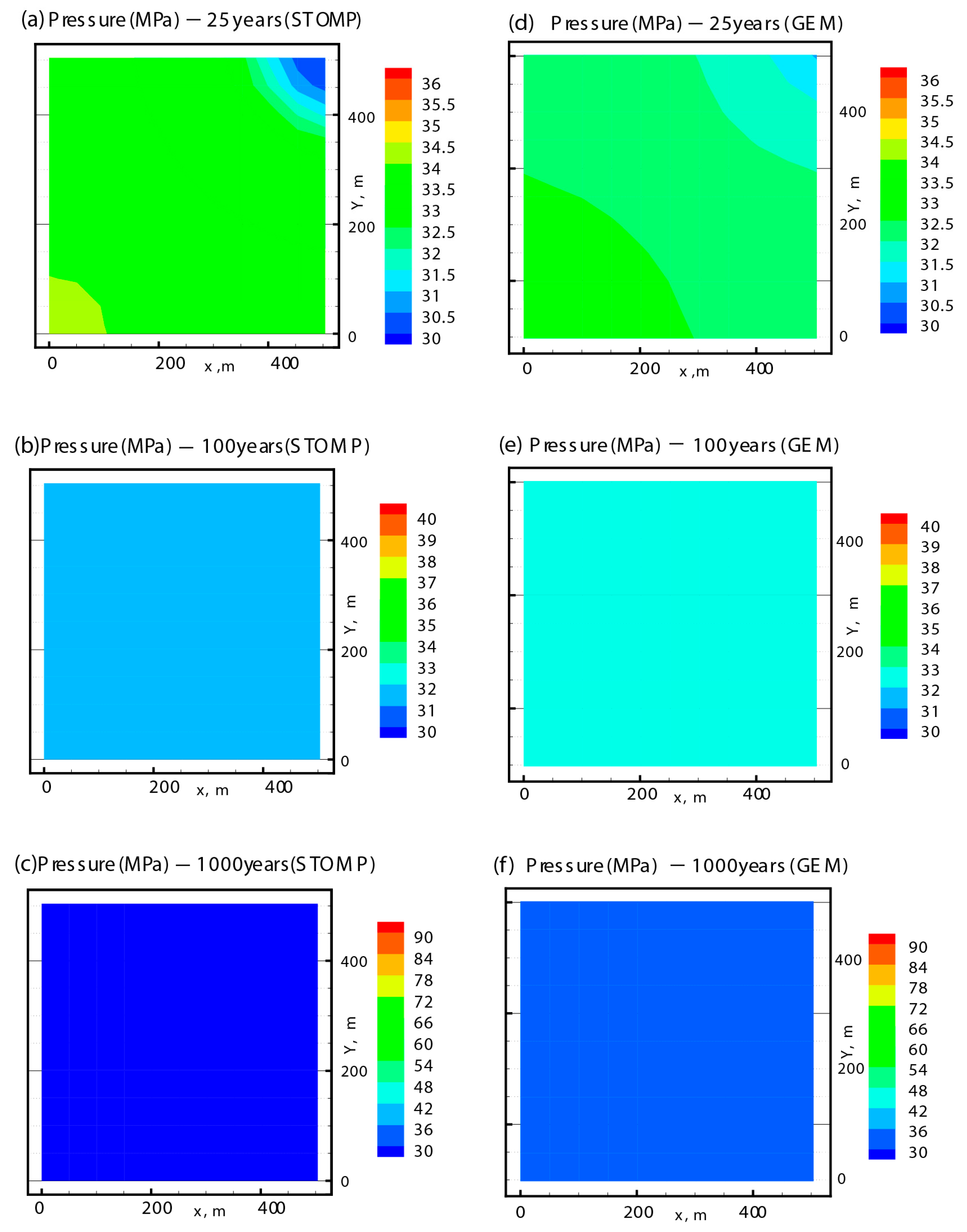
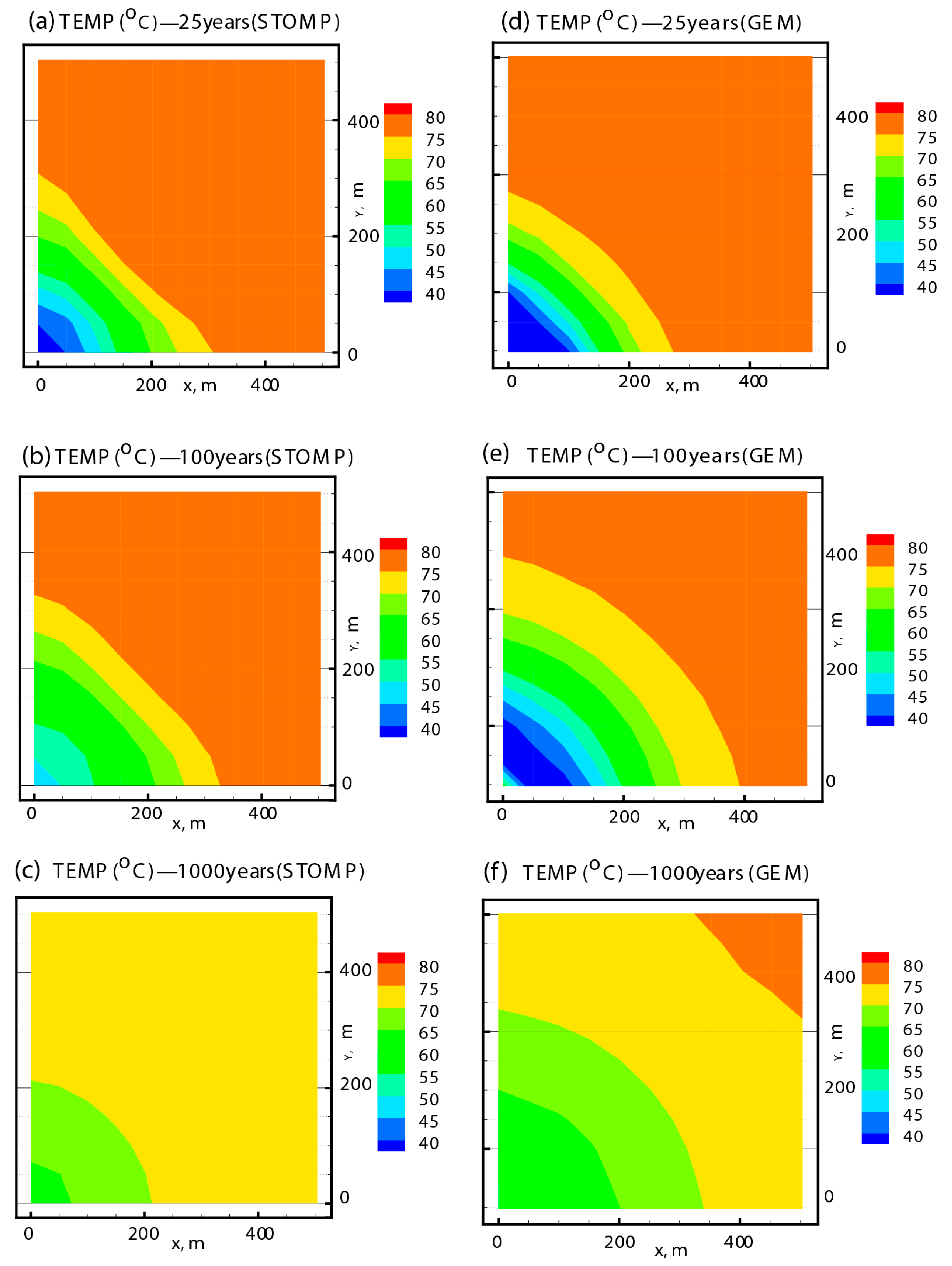
4.1.1. Temperature and Pressure Distributions

Figure 4 and Figure 5 show plan views of the evolution of reservoir pressure and temperature predicted in the STOMP-EOR, TOUGHREACT, and GEM models in the middle layer of the model grid as a result of water and CO₂ introduced through the injection well at the lower left corner of each plot. All three models predicted an increase in fluid pressure from the initial value of 30 MPa during the 25 years of injection, reaching a maximum of ~33 MPa. After the injection period ended, all three models predicted fluid pressures to decline, but not at the same rate. The fastest fluid pressure decline was predicted in the TOUGHREACT model, where fluid pressures returned to initial reservoir values within 100 years. The STOMP-EOR model predicted a slower decline in pressure, requiring several centuries for fluid pressure to return to the initial reservoir value. In the GEM model, fluid pressure had not yet returned to the initial reservoir value by the end of the 1000 year simulation time, reaching a minimum value of ~31.5 MPa.

The temperature evolutions predicted by all three models were similar. In each model, temperature near the injection well dropped from the initial reservoir temperature of 75 °C to 40 °C, the temperature of the injected fluids. Lower temperatures gradually propagated across the model domain toward the production well located at the upper left corner of the plots, continuing until the end of the simulations after 1000 years. However, after the injection well was shut in, temperature near the injection well gradually began to rise, reaching ~60 °C in the TOUGHREACT and GEM models and ~70 °C in the STOMP-EOR model after 1000 years.

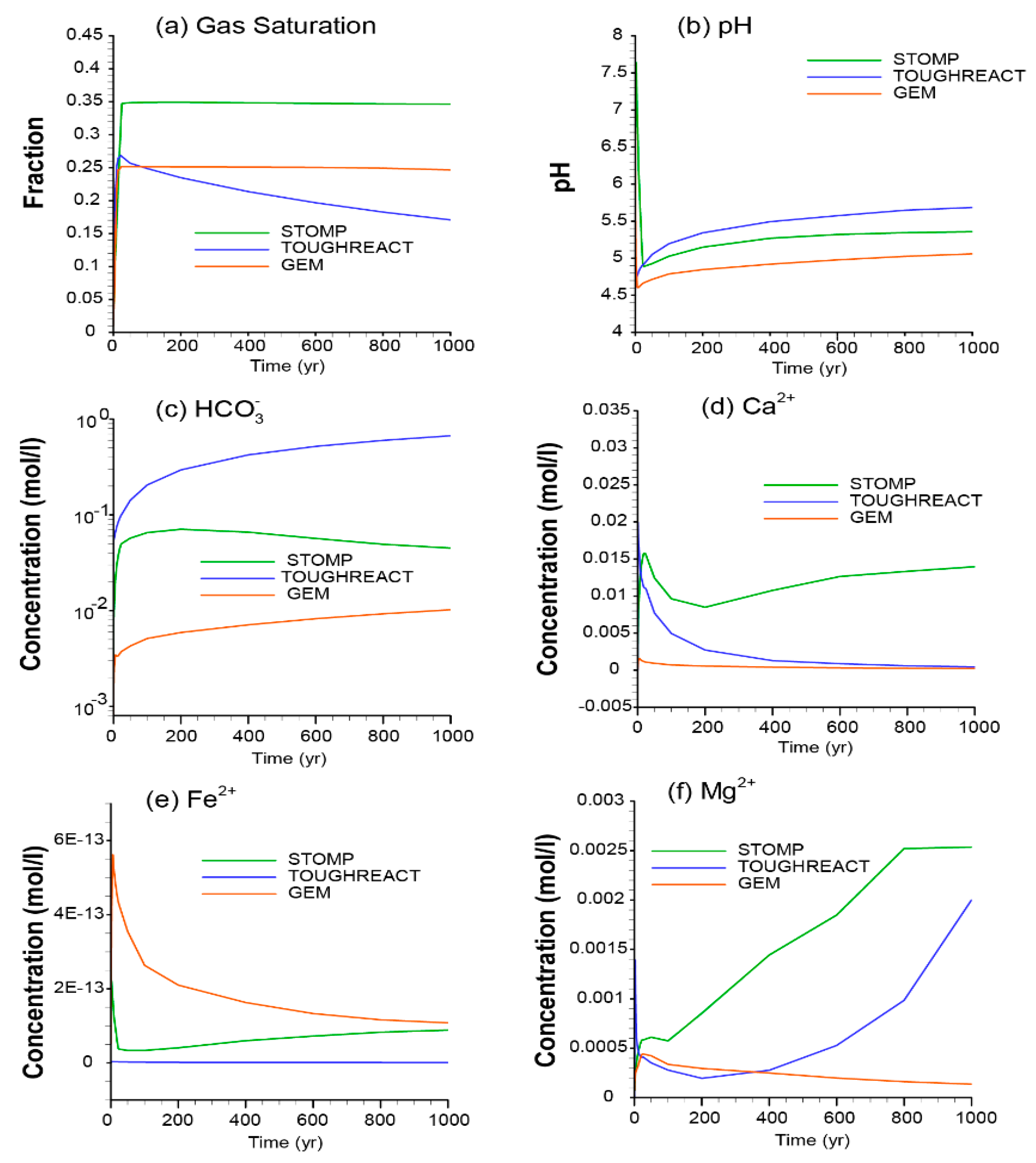
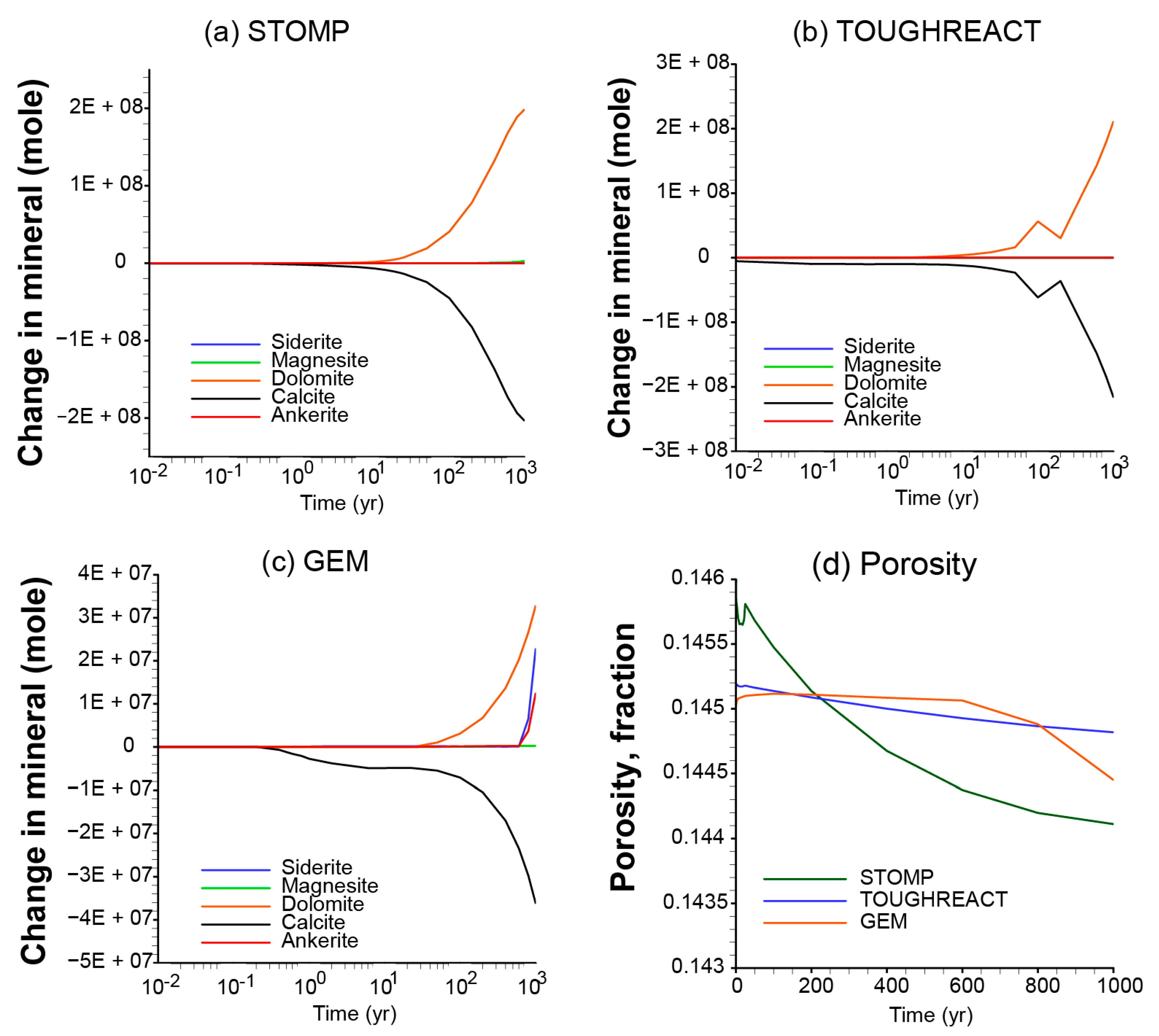
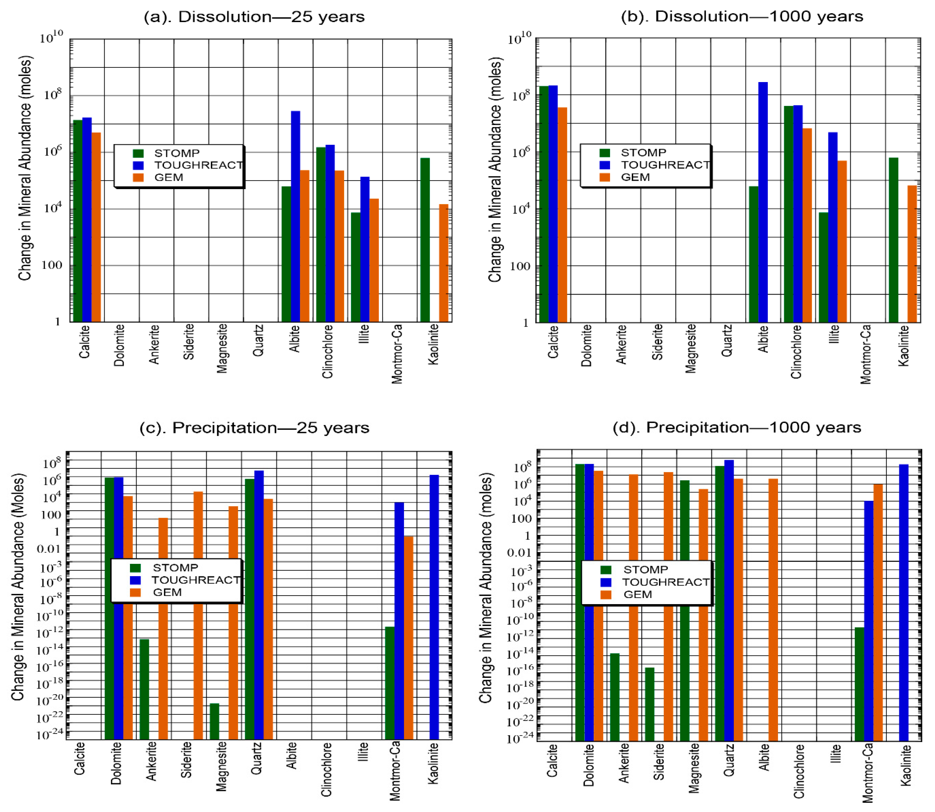
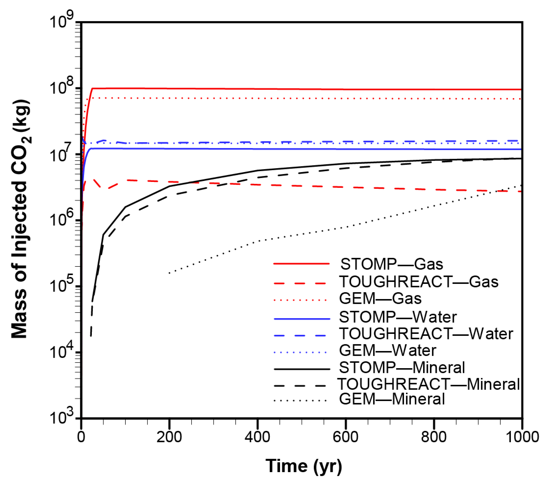
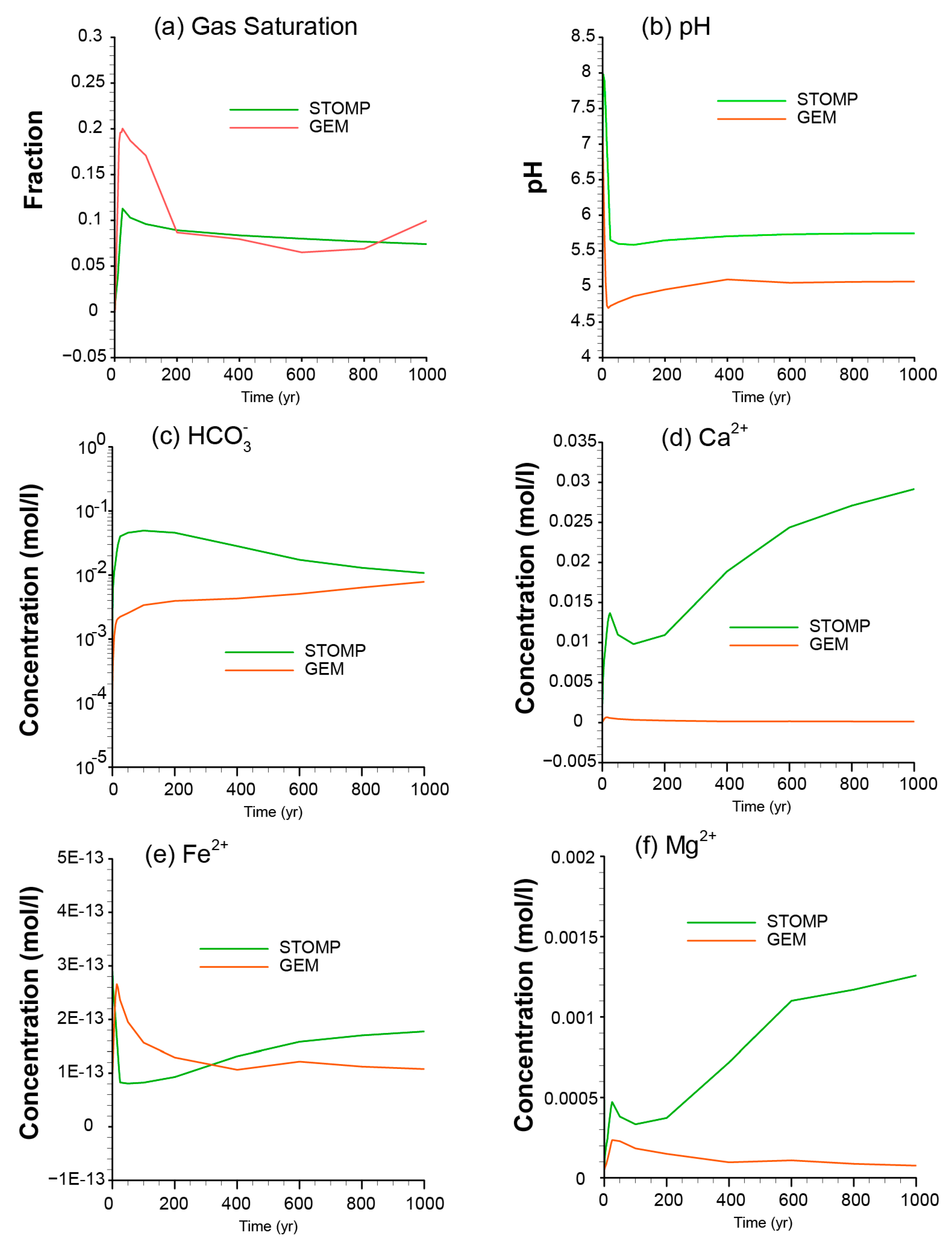
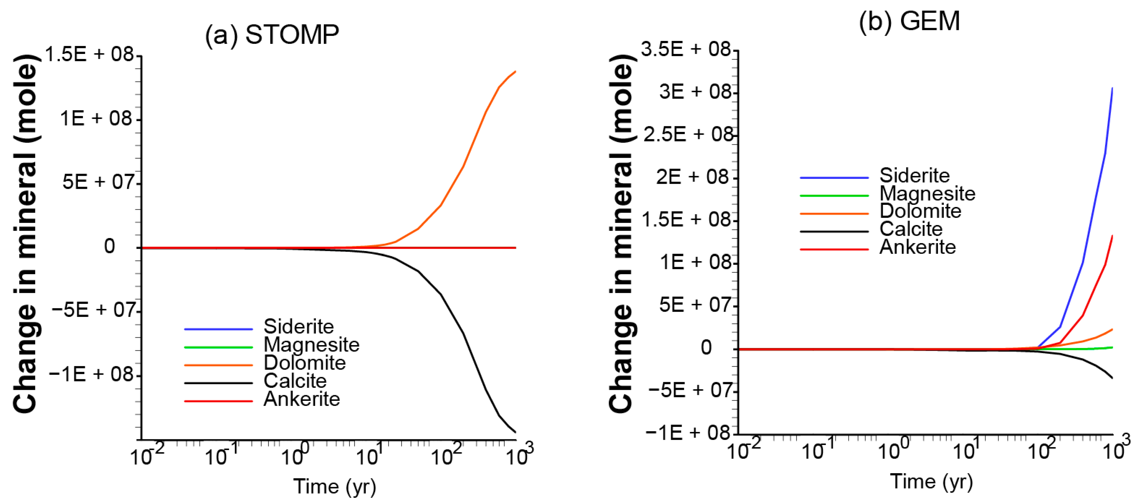
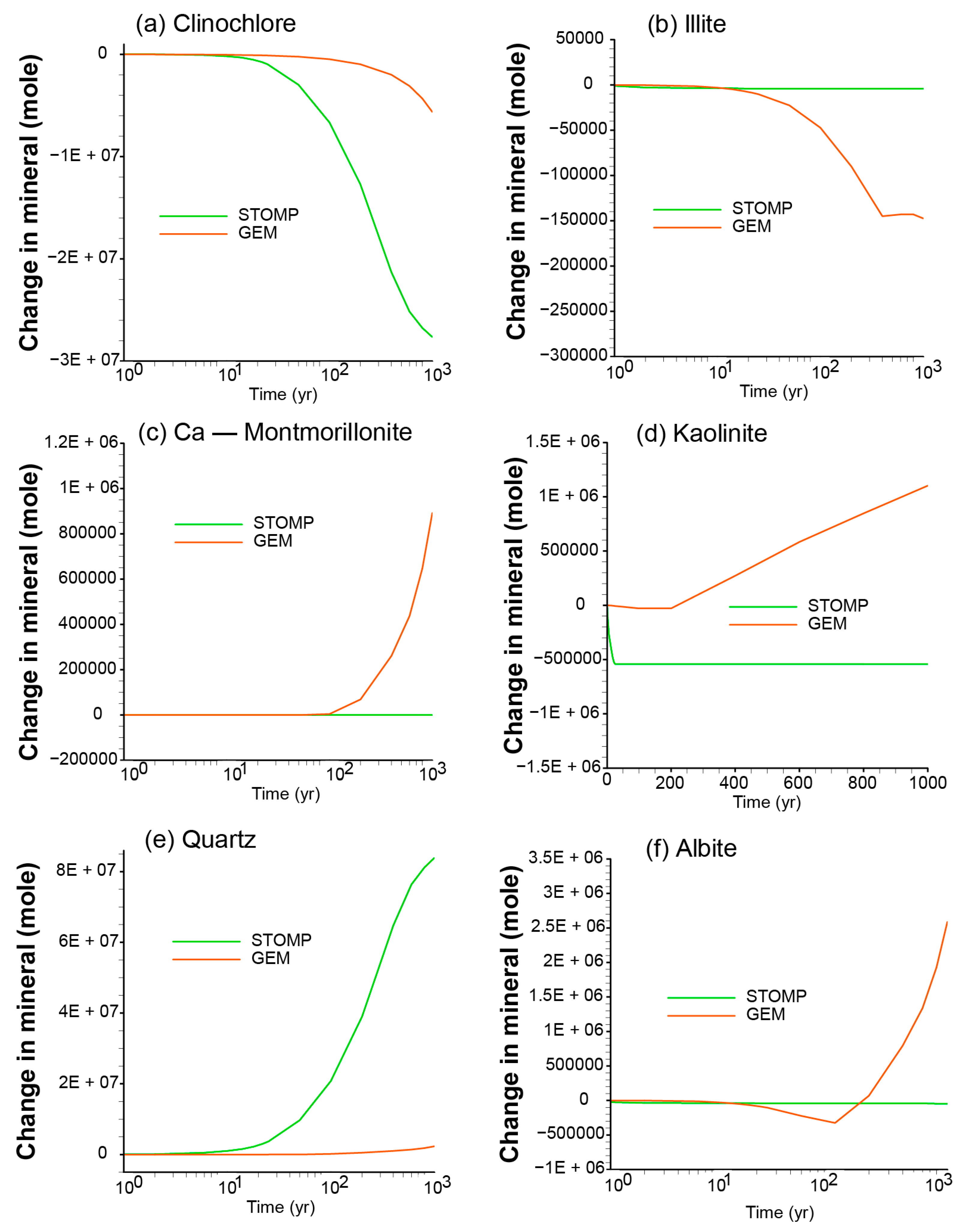
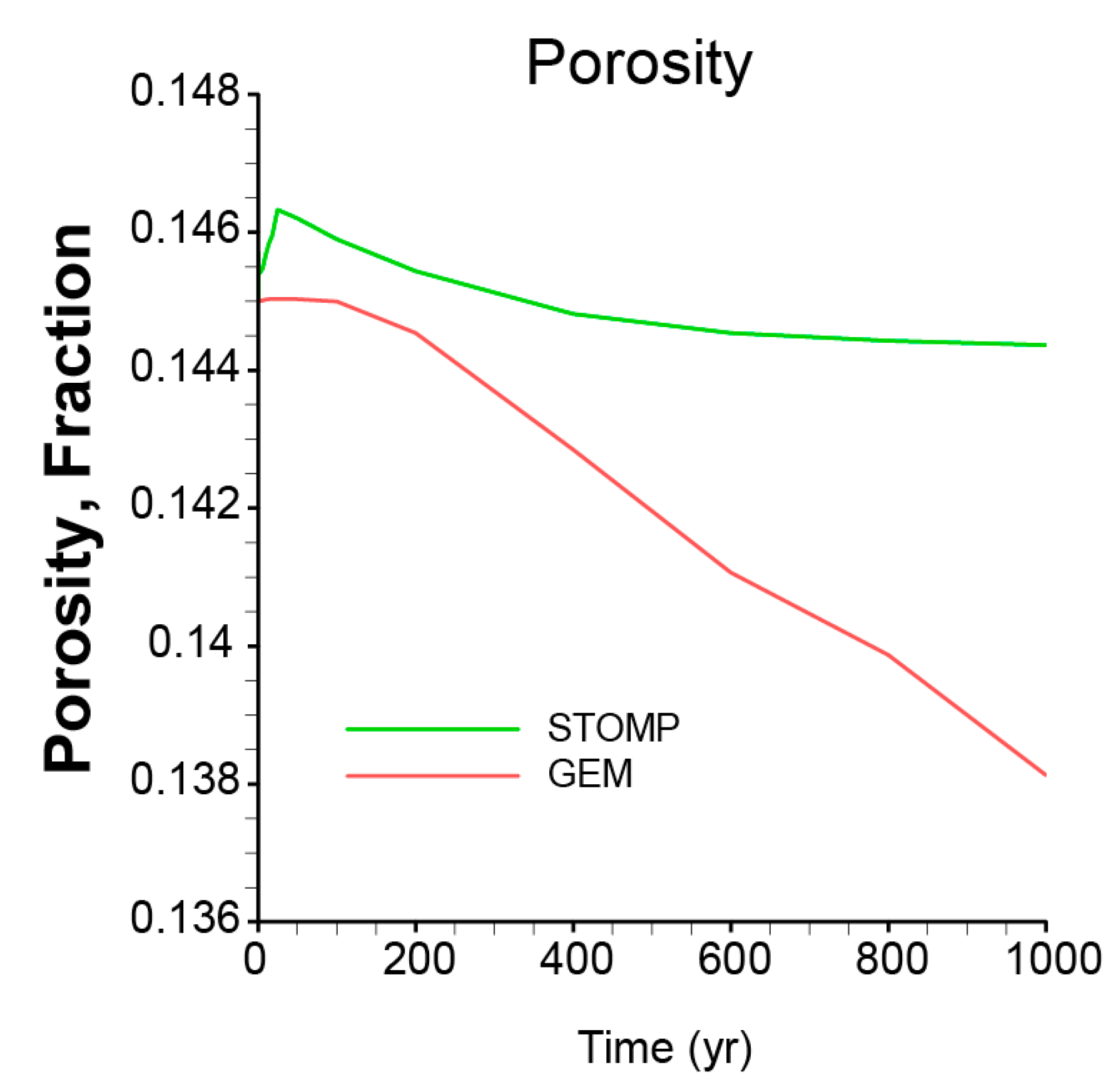
4.1.2. Evolution of Pore Fluid and Mineral Composition

In addition to altering the pressure and temperature distribution in the reservoir, the injected water and CO₂ alter the pore fluid composition of the reservoir. Figure 6 shows CO₂ gas saturation after 25, 100, 600, and 1000 years along a vertical profile between the injection well and production well as predicted by the STOMP-EOR, TOUGHREACT, and GEM models. The results of the models were most dissimilar at early times (see Figure 6a–c at 25 years), but all show CO₂ to concentrate in the upper part of the profile, which is due to buoyancy. Similar maximum gas saturations around 0.38 are also predicted by all three models. Over time the model CO₂ gas saturations converged to a similar, vertically differentiated pattern with saturations decreasing from the top of the model domain to the bottom. The CO₂ gas saturations in each model also largely stabilized after 100 years, changing little until the end of the simulations at 1000 years. However, even at longer times some differences are visible in the results. The STOMP-EOR model predicted the highest overall gas saturations and the TOUGHREACT model predicted the CO₂ gas plume not to migrate all of the way to the production well on the right boundary of the plots. The differences in gas saturation may be a function of different CO₂ solubility relationships used in the three simulators [24,25,26].

CO₂ gas saturation as a function of time is shown in Figure 7a. All three models show a sharp increase in gas saturation during the injection period. In addition, in all three models, gas saturation remains significantly elevated over the entire 1000-year simulation period, though in the TOUGHREACT model, gas saturation steadily declines after the injection well is shut in, whereas in the STOMP-EOR and GEM models, gas saturation remains relatively constant at its maximum level. The long-term persistence of this immiscible CO₂ gas phase is largely a product of the no-flow boundary conditions that encompass the model domain. Once the production well is turned off after 25 years, the CO₂ can no longer exit the model domain and can only diminish in abundance by dissolving into the formation water. Much of the injected CO₂ dissolves into the Morrow B formation water and this has a direct effect on its pH and ${\mathrm{HCO}}_3^{-}$ concentration, as indicated by Equation (5) and as shown in Figure 7b,c. The injection of CO₂ causes an immediate drop in the pH and an increase in the ${\mathrm{HCO}}_3^{-}$ concentration, though not by the same amounts. The GEM, TOUGHREACT and STOMP-EOR models predict minimum pH values of 4.6, 4.7, and 4.8, respectively, at the onset of CO₂ injection. All three models predicted a gradual increase in pH over time; this occurs within the first few years after the injection ceased until the end of the simulation. The eventual pH increase is probably caused by reactions with various minerals in the Morrow B that consume H⁺.

All three models predicted an initial increase in ${\mathrm{HCO}}_3^{-}$ concentration over time, though these concentrations varied by ~1.5 orders of magnitude among the three simulators, with the lowest concentrations predicted by the GEM model, followed by the STOMP-EOR and TOUGHREACT models, respectively. In the GEM and TOUGHREACT models, ${\mathrm{HCO}}_3^{-}$ concentration continued to rise throughout the rest of the simulation, whereas in the STOMP-EOR simulation, ${\mathrm{HCO}}_3^{-}$ concentration began to decline after about 200 years. Several competing factors affect the concentration of ${\mathrm{HCO}}_3^{-}$. Some ${\mathrm{HCO}}_3^{-}$ may be generated through the gradual dissolution of residual CO₂ gas into the formation water and by the dissolution of calcite, a native reservoir mineral, which also neutralizes pH (Equations (4) and (5); Figure 8 and Figure 9). Some ${\mathrm{HCO}}_3^{-}$ is removed from the formation water by the precipitation of other carbonate minerals such as dolomite, magnesite, and ankerite (Equations (6)–(8)).

$$\mathrm{C}{\mathrm{O}}_{2\left(\mathrm{a}\mathrm{q}\right)}+{\mathrm{H}}_2\mathrm{O}\leftrightarrow {\mathrm{H}}^{+}+\mathrm{H}\mathrm{C}{\mathrm{O}}_3^{-}$$

(4)

$${\mathrm{H}}^{+}+{\mathrm{CaCO}}_3\left(\mathrm{Calcite}\right)\to {\mathrm{Ca}}^{2+}+{\mathrm{HCO}}_3^{-}$$

(5)

$${\mathrm{Ca}}^{2+}+{\mathrm{Mg}}^{2+}+{\mathrm{HCO}}_3^{-}\to {\mathrm{CaMgCO}}_3\left(\mathrm{Dolomite}\right)+{\mathrm{H}}^{+}$$

(6)

$${\mathrm{Mg}}^{2+}+{\mathrm{HCO}}_3^{-}\to {\mathrm{MgCO}}_3\left(\mathrm{Magnesite}\right)+{\mathrm{H}}^{+}$$

(7)

$${\mathrm{Ca}}^{2+}+0.3{\mathrm{Mg}}^{2+}+0.7{\mathrm{Fe}}^{2+}+2{\mathrm{HCO}}_3^{-}\to {\mathrm{CaMg}}_{0.3}{\mathrm{Fe}}_{0.7}{\left({\mathrm{CO}}_3\right)}_2\left(\mathrm{Ankerite}\right)+2{\mathrm{H}}^{+}$$

(8)

The sharp initial drop in pH predicted by all three models during the first years of the injection period leads to the dissolution of the native reservoir minerals, calcite, albite, clinochlore, and illite in all three models. In addition, STOMP-EOR and GEM predict kaolinite to dissolve, whereas TOUGHREACT predicts kaolinite to precipitate. By the end of the 1000-year simulation period, all three models predict calcite, clinochlore, and illite to have continued to dissolve. STOMP-EOR and TOUGHREACT also predict albite to have continued to dissolve, whereas GEM predicts albite to have begun precipitating. STOMP-EOR and GEM predict kaolinite to continue to dissolve and TOUGHREACT predicts kaolinite to continue to precipitate until the end of the simulation at 1000 years.

The predicted steady dissolution of calcite by all three models does not lead to a corresponding steady increase in Ca concentration in the formation water. Rather, Ca concentration gradually decreased over time in the TOUGHREACT and GEM models, and in the STOMP-EOR model, Ca concentration increased for the first 10 years, decreased from 10 to 200 years, and then gradually increased for the remainder of the simulation. Decreases in Ca concentration were driven by the precipitation in all three models of the Ca minerals, dolomite, and Ca-montmorillonite. In the STOMP-EOR and GEM models, further Ca was removed from the formation water by the precipitation of ankerite, siderite, and magnesite. No Fe minerals were predicted to precipitate in the TOUGHREACT model. Thus, the Fe concentration of the formation water in the TOUGHREACT model remained constant over time. However, ankerite and siderite were predicted to precipitate in the STOMP-EOR and GEM models, though much more so in the GEM model. This was enough to cause a steady decrease over time in the concentration of Fe in the formation water in the GEM model, but not enough to prevent a slight increase over time in the STOMP-EOR model. The GEM model predicted a brief initial period of increase in Mg concentration in the formation water over the first 25 years, followed by a gradual decline. The initial increase in Mg concentration is probably caused by the dissolution of clinochlore. However, with increasing time, the precipitation of dolomite, ankerite, magnesite, and Ca-montmorillonite led to a net decrease in Mg concentration. In the TOUGHREACT model, the absence of dissolution of any Mg minerals during the early years of the simulation and the precipitation of dolomite caused a decrease in Mg concentration in the formation water. At later times, high levels of clinochlore dissolution caused Mg concentration in the formation water to increase. In the STOMP-EOR model, Mg concentration increased almost continuously throughout the simulation, with the exception of a brief decline between approximately 50 and 100 years. The dissolution of clinochlore is likely the main source for the Mg concentration increase.

Quartz is the only native reservoir mineral that was predicted to precipitate in all three models (Figure 9c,d). In contrast, kaolinite, another native reservoir mineral, was predicted to dissolve in the GEM and STOMP-EOR models but was predicted to precipitate in the TOUGHREACT model.

All three of the models predicted very small, nearly continuous decreases in porosity over the course of the simulations (Figure 8d). The largest porosity decrease was predicted by the STOMP-EOR model at 0.0017. These porosity changes are likely to be too small to have a significant impact on the hydraulic properties of the Morrow B Sandstone and its capacity to sequester CO₂ in either the formation water or as an immiscible gas phase.

Figure 10 shows how the three models predict the injected CO₂ to be distributed among an immiscible gas phase, the formation water, and carbonate minerals. The STOMP-EOR and GEM models predict most of the injected CO₂ to be sequestered within an immiscible gas phase throughout the 1000 years of the simulation. All three models similarly predict the formation water to be the next most important sink for the injected CO₂. Carbonate minerals are a negligible sink for the injected CO₂ in the first years of the simulation. Indeed, in the GEM model, calcite dissolution outpaces the precipitation of other carbonate minerals for the first 200 years, after which net carbonate mineral sequestration of CO₂ begins to occur. However, in all three models, carbonate minerals become an increasingly important sink for injected CO₂ over time, and by the end of the simulation after 1000 years, they approach the formation water in importance as a mineral sink. The TOUGHREACT model predicts a relatively small amount of CO₂ to be partitioned into an immiscible gas phase compared to the other two models. In fact, by the end of the 1000-year simulation period, the TOUGHREACT model predicts the immiscible gas phase to be the smallest sink for the injected CO₂. As noted for Figure 6, the differences in the amounts of immiscible CO₂ gas predicted by the three simulators may be a function of the different CO₂ solubility functions that they employ [24,25,26].

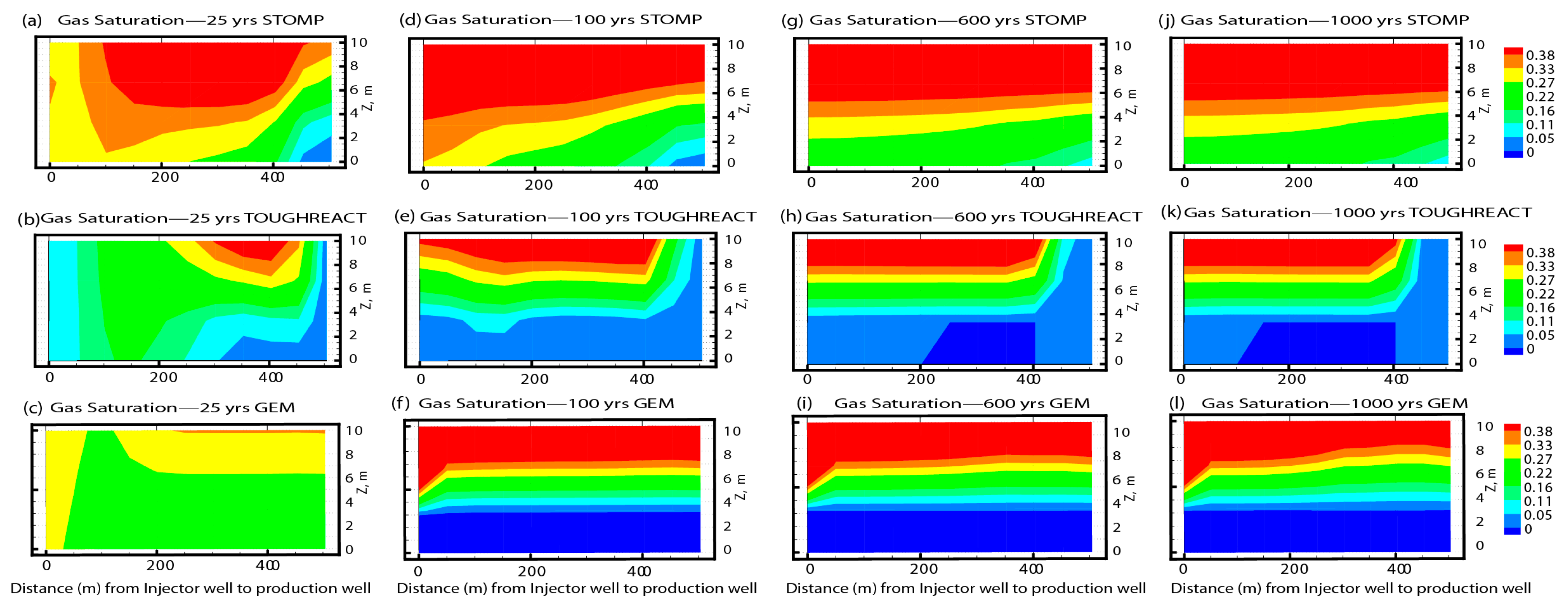
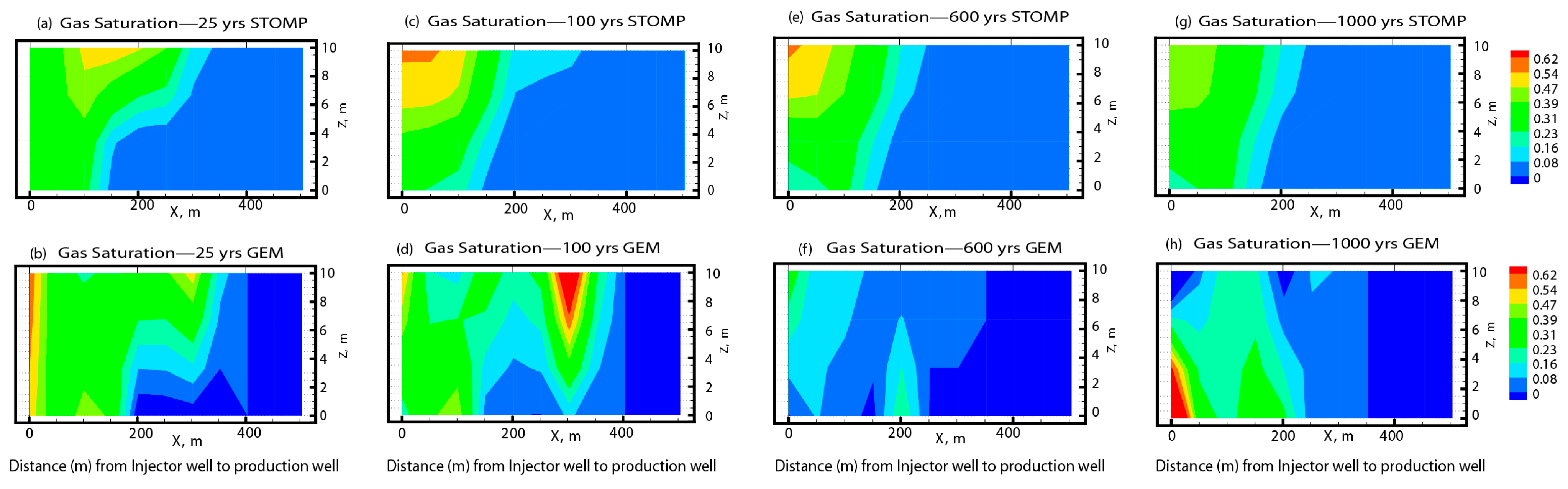
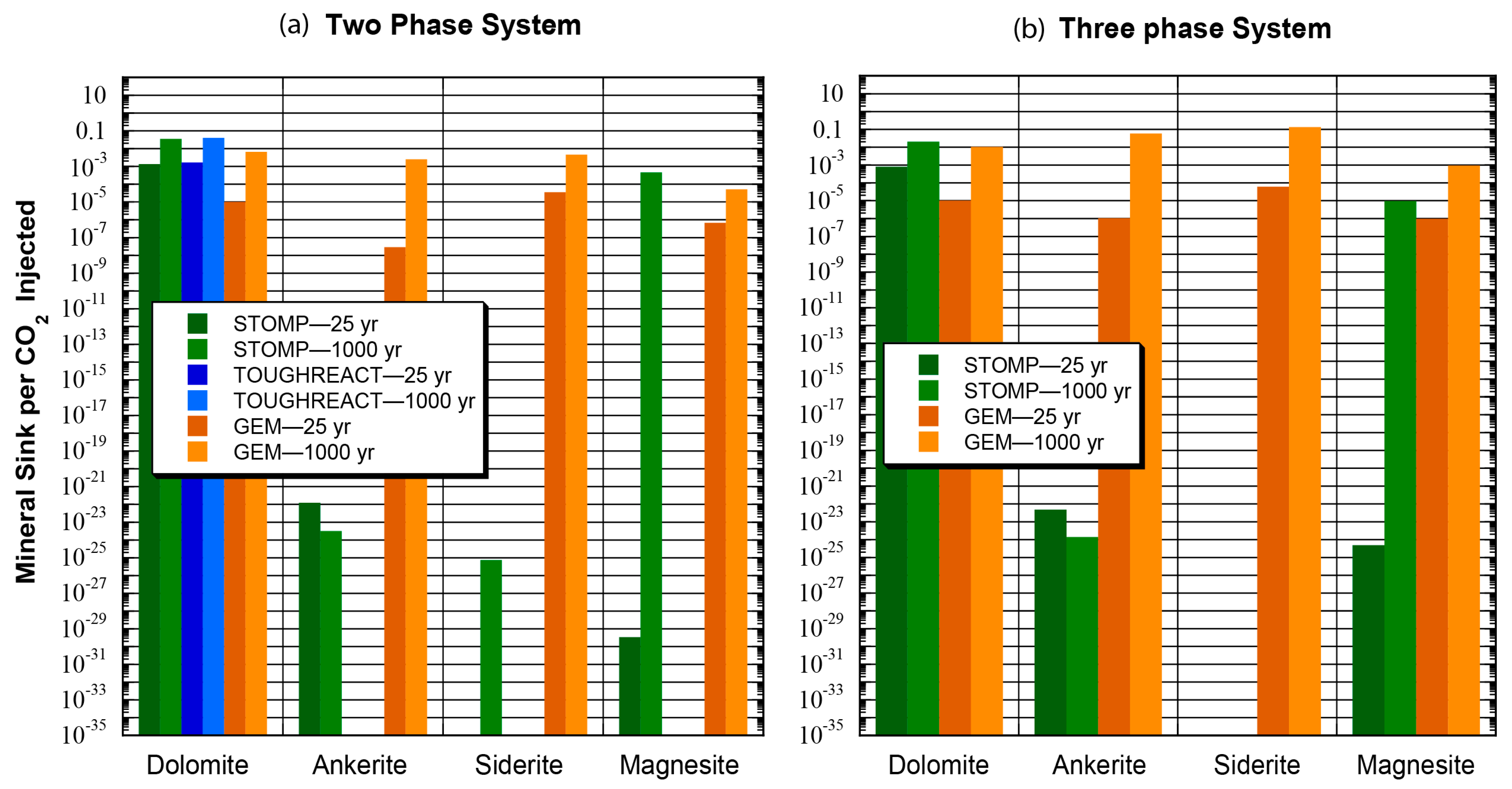
4.2. Model Scenario 2

Figure 11 and Figure 12 show plan views of the evolution of reservoir pressure and temperature predicted in the STOMP-EOR and GEM models in the middle layer of the model grid as a result of water and CO₂ introduced through the injection well at the lower left corner of each plot. The two models predicted an increase in fluid pressure from the initial value of 30 MPa during the 25 years of injection, reaching a maximum of ~34 MPa in STOMP-EOR and GEM. After injection ceased, fluid pressure was predicted to decline continuously in the STOMP-EOR model, reaching 32 MPa after 100 years and returning to the initial reservoir pressure of 30 MPa after 1000 years. A similar pressure evolution pattern was produced by the GEM model as long as siderite and ankerite were omitted from the model, as is the case for the results shown in Figure 11. Although the geochemical input parameters for siderite and ankerite were the same in the GEM and STOMP-EOR models, including siderite and ankerite in the GEM model caused pressure to continue to increase over time instead of returning to the initial value after injection ceased. This result seems to represent a limitation of the GEM model. A comparative analysis showed that the presence or absence of siderite and ankerite in the GEM model did not significantly impact the results for any model outputs except kaolinite, magnesite, and temperature. Compared to the case when siderite and ankerite were present, when siderite and ankerite were absent the GEM model predicted kaolinite abundance to be ~65% lower, magnesite precipitation was almost entirely prevented, and temperature was approximately 2.5 to 6 °C lower. The GEM results shown in the remaining plots are for the case when siderite and ankerite were included in the model.

The temperature evolutions predicted by the STOMP-EOR and GEM models in Scenario 2 are similar to one another and to the results in Scenario 1. In each model, temperature near the injection well dropped from the initial reservoir temperature of 75 to 40 °C during the injection period. After injection ceased, temperatures gradually rose and became more homogeneous across the model domain, though they had not yet completely returned to the initial reservoir temperature of 75 °C after 1000 years.

Figure 13 shows the changes in CO₂ gas saturation along a cross section between the injection well and the production well as a function of time for the STOMP-EOR and GEM models. The results of the STOMP-EOR and GEM models differ significantly in detail but have some broad similarities in that they both show a plume of CO₂ gas to migrate about halfway across the cross section by about 25 years and to remain relatively stationary thereafter. The model results of Scenario 2 differ significantly from those of Scenario 1. In Scenario 2, CO₂ gas saturation never develops a strong vertical differentiation as in Scenario 1, and the injected CO₂ plume in Scenario 2 does not arrive at the production well by the end of the simulations at 1000 years. Maximum gas saturations in Scenario 2 are higher than in Scenario 1. However, comparing Figure 14a to Figure 7a, both of which show gas saturation averaged over the entire volume of the model domain, reveals that gas saturation in Scenario 2 is overall lower than in Scenario 1. This is probably because in Scenario 2, CO₂ can dissolve in both oil and water, whereas in Scenario 1, the only pore fluid into which CO₂ can dissolve is water.

Figure 14 also shows the pH and concentrations of ${\mathrm{HCO}}_3^{-}$, Ca²⁺, Fe²⁺, and Mg²⁺ in the Morrow B formation water as a function of time, also averaged over the entire volume of the model domain. The trends in pH and concentrations of ${\mathrm{HCO}}_3^{-}$, Ca²⁺, and Mg²⁺ over time predicted by the STOMP-EOR and GEM models in Model Scenario 2 are qualitatively similar to those in Model Scenario 1 but differ significantly in their numerical values. In Model Scenario 2, the STOMP-EOR model consistently predicts higher pH and concentrations of ${\mathrm{HCO}}_3^{-}$, Ca²⁺, and Mg²⁺ compared to the GEM model, whereas the GEM model predicts higher concentrations of Fe²⁺ than in the STOMP-EOR model at early times, and the STOMP-EOR model predicts higher Fe²⁺ concentrations at later times. In Model Scenario 2, after an early increase in the GEM model, gas saturation decreases and largely parallels that predicted by the STOMP-EOR model.

The Scenario 2 STOMP-EOR and GEM models made some similar predictions about the evolution of carbonate mineral abundance (Figure 15 and Figure 16). Both models predicted continuous dissolution of calcite. The two models differ further in that large amounts of siderite, magnesite, and ankerite precipitated in the GEM model but only tiny amounts of ankerite and no siderite precipitated in the STOMP-EOR model. Minimal magnesite precipitated at early times in the STOMP-EOR model but by the end of the simulation after 1000 years, considerable magnesite had precipitated. The carbonate mineral abundances predicted in Scenario 2 resemble those in Scenario 1 in some respects. Dolomite continued to be the main carbonate mineral predicted to be precipitated in Scenario 2 in the STOMP-EOR model. In contrast, in the GEM model, siderite was the most abundant mineral precipitated followed by ankerite, dolomite, and magnesite. The presence of oil did not greatly impact the patterns of carbonate mineral precipitation in the STOMP-EOR model but appears to have greatly increased the precipitation of siderite and ankerite in the GEM model. Carbonate mineral precipitation and dissolution trends were monotonic, reaching their highest levels at the end of the 1000-year simulation period.

Changes in the abundances of non-carbonate minerals predicted by the GEM and STOMP-EOR models are shown in Figure 17. The two models predicted progressive clinochlore dissolution over time, though the GEM model predicted a much smaller amount. However, the STOMP-EOR model predicted relatively constant abundances of illite, Ca-montmorillonite, and albite, whereas the GEM model predicted a large decrease in illite abundance and a large increase in Ca-montmorillonite and albite abundance. For kaolinite, the STOMP-EOR model predicted an initial sharp dissolution event followed by relatively constant abundance, whereas the GEM model predicted precipitation throughout most of the simulation. Both models predicted continuous quartz precipitation, though the STOMP-EOR model predicted a much larger amount. The combined effects of mineral precipitation and dissolution were nearly in balance in the STOMP-EOR model, with a small porosity increase of ~0.001 predicted during the 25 year injection period, about half of which was then gradually eliminated over the remainder of the 1000 year simulation (Figure 18). The GEM model did not predict porosity to change during the injection period, but after about 100 years, porosity decreased steadily from an initial value of ~0.145 to ~0.138 after 1000 years.

Figure 19 shows how the injected CO₂ is distributed among an immiscible gas phase, oil, formation water, and carbonate minerals. Both the GEM and STOMP-EOR model predicted oil to be the largest sink for the injected CO₂, with the GEM model predicting higher amounts of CO₂ dissolution in oil than the STOMP-EOR model. Both models predicted less CO₂ to occur as immiscible gas than to dissolve in oil, and less CO₂ to dissolve in the formation water than to occur as immiscible gas. In addition, the temporal trends of CO₂ occurring in immiscible gas strongly resembled one another in the two models, as did the temporal trends of CO₂ dissolved in formation water. As for Model Scenario 1, in Model Scenario 2 carbonate minerals sequester only a small fraction of the injected CO₂, though the amount that they sequester continuously increases over time. By the end of the 1000-year simulation, the STOMP-EOR model predicts the amount of CO₂ to be sequestered in carbonate minerals to be close to the amounts occurring in immiscible gas and the formation water. In the GEM model, CO₂ sequestration in carbonate minerals has increased so much by the end of the simulation that this amount exceeds the amounts in all other CO₂ sinks except oil.

5. Discussion

The present study showed that although the models for the different simulators in each scenario were set up in the same way, they produced some significantly different results. In Model Scenario 1, the STOMP-EOR, TOUGHREACT, and GEM models predicted similar evolutions in temperature and pressure, though the pressures in the GEM model were approximately 1–2 MPa higher after 1000 years than in the other two models. This may have driven slightly higher concentrations of CO₂ into solution in the formation water in the GEM model, which would then account for its generally slightly lower pH. All three models in Scenario 1 predicted calcite to dissolve, which is a consequence of the lowering of the pH due to the injection of CO₂. However, the lower pH predicted by the GEM model corresponds with its lower overall amount of carbonate mineral precipitation compared to the other two models.

In Scenario 1, the three models also predicted significant differences in the abundances of non-carbonate minerals. The overall net changes in mineral abundances, though, were similar enough to cause similar decreasing trends in porosity over time, amounting to only about a tenth of a percent over the 1000 years of the simulation for the reservoir as a whole. Such a small change in porosity would cause a similarly small change in permeability of only tenths of a percent, meaning that the hydraulic properties and behavior of the Morrow B reservoir as a whole would not be expected to change significantly as a result of the planned CO₂ injection.

In Scenario 2, despite the differences in predicted pressures, the amount of CO₂ predicted by GEM to dissolve into water and oil does not differ much from the amount predicted by STOMP-EOR. The pH is consistently lower in the GEM model than in the STOMP-EOR model, but this does not consistently suppress the precipitation of carbonate minerals in the GEM models. Instead, overall, more carbonate mineral precipitation is predicted to occur in the GEM model than in the STOMP-EOR model. This contributes to the greater decrease in porosity predicted by the GEM model than by the STOMP-EOR model, though in both models the porosity decrease is relatively small and not enough to cause significant changes in the hydraulic properties of the reservoir as a whole.

Some of the differences in predicted mineral abundances between the GEM model and the other two models may pertain to GEM’s use of damping factors for mineral precipitation and dissolution reactions. The damping factors are multipliers applied to the reaction rates in order to aid convergence and are allowed to vary between 0 and 1000. According to the CMG-GEM user’s guide [27], damping factors for mineral reactions are justified because published reaction rate parameters in the literature, such as the rate constant and reactive surface area, are often measured on a core scale in the lab. To use these parameter values appropriately in a field-scale model, the values must be upscaled corresponding to the larger grid block sizes and the scale of the model. When laboratory-derived reaction parameters are used without upscaling, then the resultant reaction rates become spuriously high, which causes numerical convergence difficulties during the simulation. Thus, specifying mineral reaction damping factors reduces the reaction rates to more realistic values, which also helps the model to converge better. In the present study, a damping factor of 0.001 was used in the GEM models, the maximum value that allowed the models to converge. In contrast, the STOMP-EOR and TOUGHREACT models converged without damping factors.

6. Summary and Conclusions

Two model scenarios for CO₂ injection into the Morrow B Sandstone in the Farnsworth Unit were investigated in the present study. In Model Scenario 1, water was the only pore fluid initially present. In Model Scenario 2, water and petroleum were both initially present as pore fluids. Model Scenario 1 allowed a comparison of the performance of the TOUGHREACT, STOMP-EOR, and GEM simulators to be made. Model Scenario 2 allowed a comparison of the STOMP-EOR and GEM simulators to be made. Both model scenarios also provided fundamental insights into the behavior and effects of the injected CO₂. In Model Scenario 1, the models from the three simulators predicted a similar rise in pressure up to ~33 MPa during the 25-year injection period but predicted different rates of pressure decline after injection ceased. The three models predicted similar patterns of reservoir cooling to a minimum temperature of 40 °C near the injection well, followed by similar patterns of temperature homogenization after injection ceased. All three models predicted the long-term persistence of an immiscible CO₂ gas phase but differed by up to approximately a factor of two in the amounts that persisted. All three models predicted sharp declines in pH from the initial value of 7 to between approximately 4.6 and 4.9, gradually rising with increasing time due to water–rock reactions. All three models predicted calcite to dissolve through the simulations and for dolomite to be the main carbonate mineral sink for the injected CO₂. However, the models differed in the amounts of other carbonate minerals (siderite, magnesite, and ankerite) that were predicted to precipitate. The three models differed more strongly in terms of their predictions about silicate minerals. All three models consistently predicted quartz and Ca-montmorillonite to precipitate and clinochlore and illite to dissolve, but in significantly different amounts. However, the predicted differences in neither silicate nor carbonate mineral abundance were sufficient to cause large changes in porosity, which showed a slight decreasing trend in all three models. The STOMP-EOR and GEM models predicted similar amounts of immiscible CO₂ gas to be the main sink for the injected CO₂ over the 1000 years of the simulations, while the amount predicted by the TOUGHREACT model was much lower and not the main injected CO₂ sink. All three models predicted similar amounts of injected CO₂ to be sequestered in aqueous solution. Carbonate minerals were predicted by all three models to be a smaller sink for injected CO₂ than the formation water, though carbonate minerals were the only CO₂ sink that grew in magnitude over time.

In Model Scenario 2, only the GEM and STOMP-EOR simulators were tested. Both the GEM and STOMP-EOR models made similar predictions of initial cooling around the injection well followed by thermal homogenization that were made in Model Scenario 1. The STOMP-EOR model made a qualitatively similar prediction of pressure evolution as in Model Scenario 1. However, the GEM model predicted an ongoing increase in pressure after injection ceased until the end of the simulation at 1000 years unless the minerals siderite and ankerite were removed from the model. The GEM model predicted gas saturations to be about twice as high as the STOMP-EOR model during the early years of the simulation, but after about 200 years the two models predicted similar gas saturations. Both models predicted lower overall gas saturations in Model Scenario 2 than in Model Scenario 1. Both the GEM and the STOMP-EOR models predicted a sharp decrease in pH during injection in Model Scenario 2. However, whereas the GEM model predicted a similar minimum pH of 4.6 in the two model scenarios, the STOMP-EOR model predicted a significantly higher minimum pH of 5.6 in Model Scenario 2 compared to the minimum pH of 4.9 it predicted in Model Scenario 1. Both models continued to predict calcite to dissolve continuously in Model Scenario 2. The STOMP-EOR model again predicted dolomite to be the main carbonate mineral sink for injected CO₂, whereas the GEM model predicted siderite and ankerite to be more important mineral sinks. The two models predicted significant differences in silicate mineral abundance. Together, the differences in carbonate and silicate mineral abundances led to significant differences in porosity, with the STOMP-EOR model predicting an overall porosity decrease to 0.1445 and the GEM model to about 0.1385. Overall, CO₂ injection was predicted to have a small impact on porosity over 1000 years. Both models in Scenario 2 predicted oil to be the main sink for injected CO₂. Both models predicted immiscible gas and the formation water, respectively, to be smaller sinks for injected CO₂. STOMP-EOR predicted carbonate minerals to be the smallest sink for injected CO₂. For GEM this was also true for about the first 300 years of the simulation, but the end of the 1000 years of the simulation, GEM predicted carbonate minerals to be the second most important sink for injected CO₂ after oil.

Although the models in each scenario were set up the same and although the model results have many qualitative similarities, the models differ in many of the details of their results. The results indicate that executing models on multiple simulators can more clearly identify areas of confidence as well as uncertainty in projected outcomes in the field.

References

1. Balch, R.; McPherson, B.; Grigg, R. Overview of a Large Scale Carbon Capture, Utilization, and Storage Demonstration Project in an Active Oil Field in Texas, USA. Energy Procedia 2016, 114, 5874–5887. [Google Scholar] [CrossRef]
2. Balch, R.; McPherson, B. Integrating Enhanced Oil Recovery and Carbon Capture and Storage Projects: A Case Study at Farnsworth Field, Texas. In SPE Western Regional Meeting; OnePetro: Anchorage, AK, USA, 2016. [Google Scholar]
3. Ahmmed, B. Numerical Modeling of CO2-Water-Rock Interactions in the Farnsworth, Texas Hydrocarbon Unit, USA. 2015, Volume 3, pp. 54–67. Available online: https://mospace.umsystem.edu/xmlui/bitstream/handle/10355/46985/research.pdf?sequence=2 (accessed on 3 May 2021).
4. Xu, T.; Sonnenthal, E.; Spycher, N.; Pruess, K. TOUGHREACT User’s Guide: A Simulation Program for Non-Isothermal Multiphase Reactive Geochemical Transport in Variably Saturated Geologic Media; V1.2.1-LBNL-55460-2008; Lawrence Berkeley National Lab. (LBNL): Berkeley, CA, USA, 2008; Volume 32, pp. 1–206.
5. Pan, F.; McPherson, B.J.; Esser, R.; Xiao, T.; Appold, M.S.; Jia, W.; Moodie, N. Forecasting evolution of formation water chemistry and long-term mineral alteration for GCS in a typical clastic reservoir of the Southwestern United States. Int. J. Greenh. Gas Control 2016, 54, 524–537. [Google Scholar] [CrossRef] [Green Version]
6. Gallagher, S.R. Depositional and Diagenetic Controls On Reservoir Heterogeneity: Upper Morrow Sandstone. Master’s Thesis, Farnsworth Unit, Ochiltree County, TX, USA, 2014; pp. 1–233. [Google Scholar]
7. Khan, R.H. Evaluation of the geologic CO2 sequestration potential of the Morrow B sandstone in the Farnsworth, Texas hydrocarbon field using reactive transport modeling. Am. Geophys. Union 2017. [Google Scholar] [CrossRef]
8. Sun, Q.; Ampomah, W.; Kutsienyo, E.J.; Appold, M.; Adu-Gyamfi, B.; Dai, Z.; Soltanian, M.R. Assessment of CO2 trapping mechanisms in partially depleted oil-bearing sands. Fuel 2020, 278, 118356. [Google Scholar] [CrossRef]
9. Nghiem, L.; Sammon, P.; Grabenstetter, J.; Ohkuma, H. Modeling CO2 Storage in Aquifers with a Fully-Coupled Geochemical EOS Compositional Simulator. In SPE/DOE Symposium on Improved Oil Recovery; No. SPE 89474 Modeling; OnePetro: Tulsa, OK, USA, 2004; pp. 1–16. [Google Scholar]
10. CMG. GEM Compositional and Unconventional Simulator. 2021. Available online: https://www.cmgl.ca/gem (accessed on 10 August 2021).
11. White, M.; McPherson, B.; Grigg, R.; Ampomah, W.; Appold, M. Numerical Simulation of Carbon Dioxide Injection in the Western Section of the Farnsworth Unit. Energy Procedia 2014, 63, 7891–7912. [Google Scholar] [CrossRef] [Green Version]
12. Span, R.; Wagner, W. A New Equation of State for Carbon Dioxide Covering the Fluid Region from the Triple-Point Temperature to 1100 K at Pressures up to 800 MPa. J. Phys. Chem. Ref. Data 1996, 25, 1509–1596. [Google Scholar] [CrossRef] [Green Version]
13. Xu, T.; Apps, J.A.; Pruess, K. Reactive geochemical transport simulation to study mineral trapping for CO2 disposal in deep arenaceous formations. J. Geophys. Res. Solid Earth 2003, 108. [Google Scholar] [CrossRef]
14. Munson, T.W. Depositional, Diagenetic, and Production History of the upper Morrowan Buckhaults Sandstone, Farnsworth Field Ochiltree County Texas. OCGS-Shale Shak. Dig. XII 1989, XXXX–XXXXI, 2–20. [Google Scholar]
15. Heath, J.E.; Dewers, T.A.; Mozley, P.S. Characteristics of the Farnsworth Unit, Ochiltree County; Southwest Partnership CO2 Storage-EOR Project: Ochiltree, TX, USA, 2015. [Google Scholar]
16. Ross-Coss, D.; Ampomah, W.; Cather, M.; Balch, R.S.; Mozley, P.; Rasmussen, L. An Improved Approach for Sandstone Reservoir Characterization. In Proceedings of the SPE Western Regional Meeting, Anchorage, AK, USA, 23–26 May 2016. [Google Scholar]
17. Trujillo, N.A. Influence of Lithology and Diagenesis on Mechanical and Sealing Properties of the Thirteen Finger Limestone and Upper Morrow Shale, Farnsworth Unit, Ochiltree County, Texas; ProQuest: Ann Abor, MI, USA, 2017. [Google Scholar]
18. White, M.D.; Oostrom, M. User Guide: Subsurface Transport Over Multiple Phases. June 2006 Contract: DE-AC05-76RL01830. Available online: https://www.pnnl.gov/main/publications/external/technical_reports/PNNL-15782.pdf (accessed on 20 August 2021).
19. Xu, T.; Apps, J.A.; Pruess, K. Numerical simulation of CO2 disposal by mineral trapping in deep aquifers. Appl. Geochem. 2004, 19, 917–936. [Google Scholar] [CrossRef]
20. CMG. CMOST User’s Guide: CO2 Sequestration Using GEM. 2018. Available online: https://www.cmgl.ca/training/co2-sequestration-using-gem (accessed on 20 August 2021).
21. Ahmmed, B.; Appold, M.S.; Fan, T.; McPherson, B.J.O.L.; Grigg, R.B.; White, M.D. Chemical Effects of Carbon Dioxide Sequestration in the Upper Morrow Sandstone in the Farnsworth, Texas, hydrocarbon unit. Environ. Geosci. 2016, 23, 81–93. [Google Scholar] [CrossRef]
22. Palandri, J.L.; Kharaka, Y.K. A Compilation of Rate Parameters of Water-Mineral Interaction Kinectics for Application to Geochemical Modelling. U.S. Geol. Surv. Open File Rep. 2004, 271, 1–70. [Google Scholar]
23. Gunda, D.; Ampomah, W.; Grigg, R.; Balch, R. Reservoir Fluid Characterization for Miscible Enhanced Oil Recovery. Carbon Management Technology Conference; OnePetro: Sugarland, TX, USA, 2015. [Google Scholar]
24. Battistelli, A.; Calore, C.; Pruess, K. The simulator TOUGH2/EWASG for modelling geothermal reservoirs with brines and non-condensible gas. Geothermics 1997, 26, 437–464. [Google Scholar] [CrossRef]
25. Spycher, N.; Pruess, K. CO2-H2O Mixtures in the Geological Sequestration of CO2. II. Partitioning in Chloride Brines at 12–100 °C and up to 600 bar. Geochim. Cosmochim. Acta 2005, 69, 3309–3320. [Google Scholar] [CrossRef]
26. Harvey, A. Semiempirical correlation for Henry’s constants over large temperature ranges. AIChE J. 1996, 42, 1491–1494. [Google Scholar] [CrossRef]
27. CMG-GEM. GHG-GEM Users Guide: GHG Option—Damping Factor for Reactions Other than Chemical *MRDAMP-ALL, *MRDAMP. 2020. Available online: https://www.cmgl.ca/resources (accessed on 20 August 2021).
Figure 1. Location of the Farnsworth Unit and the Anadarko basin within the seven-state region of the SWP.
Energies 14 05337 g001
Figure 2. Pennsylvanian stratigraphic sequence of the of Farnsworth Unit. From Gallagher [6].
Energies 14 05337 g002
Figure 3. Model spatial domains. (a) Areal extent of the FWU. Black circles represent production wells. Black circles with arrows represent injection wells. The dashed rectangle represents the area of the five-spot pattern considered in the present study. (b) Plan view of the five-spot well pattern on which the present study was based. The blue shaded rectangle represents the area of the model domain. (c) Numerical grid corresponding to the blue shaded area in panel (b).
Energies 14 05337 g003
Figure 4. Plan views of the evolution of fluid pressure in the middle cell layer of the model grid predicted by the STOMP-EOR models (ac), TOUGHREACT models (df), and GEM models (gi) after 25, 100, and 1000 years.
Energies 14 05337 g004
Figure 5. Plan views of the evolution of temperature in the middle cell layer of the model grid predicted by the STOMP-EOR models (ac), TOUGHREACT models (df), and GEM models (gi) after 25, 100, and 1000 years.
Energies 14 05337 g005
Figure 6. CO2 gas saturation along a vertical cross section between the injection well and the producing well after 25 years predicted by the STOMP-EOR, TOUGHREACT, and GEM models after (ac) 25 years, (df) 100 years, (gi) 600 years, and (jl) 1000 years.
Energies 14 05337 g006
Figure 7. Simulated (a) gas saturation; (b) pH; and concentrations of (c) HCO3, (d) Ca2+, (e) Fe2+, and (f) Mg2+ as a function of time integrated over the entire model domain.
Energies 14 05337 g007
Figure 8. Simulated changes in carbonate minerals abundances (a) STOMP-EOR, (b) TOUGHREACT, (c) GEM, and changes in fraction. (d) Porosity as a function of time integrated over the entire model domain.
Energies 14 05337 g008
Figure 9. Simulated changes in mineral volume integrated over the entire model domain due to dissolution after (a) 25 years, (b) 1000 years, and due to precipitation after (c) 25 years and (d) 1000 years predicted by the STOMP-EOR, TOUGHREACT, and GEM models.
Energies 14 05337 g009
Figure 10. Mass of injected CO2 that is sequestered in an immiscible gas phase, in the formation water, and in carbonate minerals as predicted by the STOMP-EOR, GEM, and TOUGHREACT models in Model Scenario 1.
Energies 14 05337 g010
Figure 11. Plan views of the evolution of fluid pressure in the middle cell layer of the model grid predicted by the STOMP-EOR models (ac) and GEM models (df) after 25, 100, and 1000 years, respectively. The GEM results are for ankerite and siderite omitted from the model, as the inclusion of these minerals in the GEM model produced unrealistically high pressures that steadily increased over time.
Energies 14 05337 g011
Figure 12. Plan views of the evolution of temperature in the middle cell layer of the model grid predicted by the STOMP-EOR models (ac) and GEM models (df) after 25, 100, and 1000 years, respectively.
Energies 14 05337 g012
Figure 13. CO2 gas saturation and porosity along a vertical cross section between the injection well and the producing well predicted by the STOMP-EOR and GEM models, respectively, after (a,b) 25 years, (c,d) 100 years, (e,f) 600 years, and (g,h) 1000 years.
Energies 14 05337 g013
Figure 14. Simulated (a) gas saturation; (b) pH; and concentrations of (c) H C O 3 , (d) Ca2+, (e) Fe2+, and (f) Mg2+ as a function of time averaged over the entire model domain.
Energies 14 05337 g014
Figure 15. Simulated changes in carbonate mineral abundances for the (a) STOMP-EOR model and (b) GEM model as a function of time averaged over the entire model domain.
Energies 14 05337 g015
Figure 16. Predicted carbonate mineral abundances for (a) Scenario 1 and (b) Scenario 2 after 25 and 1000 years.
Energies 14 05337 g016
Figure 17. Changes in mineral abundance predicted by the STOMP-EOR and GEM models for (a) clinochlore, (b) illite, (c) Ca-montmorillonite, (d) kaolinite, (e) quartz, and (f) albite.
Energies 14 05337 g017
Figure 18. Simulated changes in porosity as a function of time averaged over the entire model domain as predicted by the STOMP-EOR and GEM models.
Energies 14 05337 g018
Figure 19. Mass of injected CO2 that is sequestered in oil, in an immiscible gas phase, in the formation water, and in carbonate minerals as predicted by the STOMP-EOR and GEM models in Model Scenario 2.
Energies 14 05337 g019