
Contaminant Source Identification from Finite Sensor Data: Perron–Frobenius Operator and Bayesian Inference

1
Pacific Northwest National Laboratory, Electricity Infrastructure & Buildings Division, Richland, WA 99354, USA
2
Department of Mechanical Engineering, Clemson University, Clemson, SC 29634, USA
3
Department of Mechanical Engineering, Iowa State University, Ames, IA 50010, USA
*
Author to whom correspondence should be addressed.
Energies 2021, 14(20), 6729; https://doi.org/10.3390/en14206729
Submission received: 18 August 2021
/
Revised: 4 October 2021
/
Accepted: 10 October 2021
/
Published: 15 October 2021
(This article belongs to the Special Issue Building Energy and Environment)
Abstract
:Sensors in the built environment ensure safety and comfort by tracking contaminants in the occupied space. In the event of contaminant release, it is important to use the limited sensor data to rapidly and accurately identify the release location of the contaminant. Identification of the release location will enable subsequent remediation as well as evacuation decision-making. In previous work, we used an operator theoretic approach—based on the Perron–Frobenius (PF) operator—to estimate the contaminant concentration distribution in the domain given a finite amount of streaming sensor data. In the current work, the approach is extended to identify the most probable contaminant release location. The release location identification is framed as a Bayesian inference problem. The Bayesian inference approach requires considering multiple release location scenarios, which is done efficiently using the discrete PF operator. The discrete PF operator provides a fast, effective and accurate model for contaminant transport modeling. The utility of our PF-based Bayesian inference methodology is illustrated using single-point release scenarios in both two and three-dimensional cases. The method provides a fast, accurate, and efficient framework for real-time identification of contaminant source location.
1. Introduction
The accidental or intentional release of pollutants in the built environment presents a serious risk factor to occupant health and safety. In addition to common pollutants—like CO, volatile organic chemical compounds (VOCs), atmospheric particulate matter (pollens), and microbial contaminants—which affect indoor air quality (IAQ) [1], maliciously released pollutants in enclosed public spaces can cause human fatalities. Such events include release of chemical and biological weapons (CBW) or the transmission of infectious diseases (TID) with examples being the sarin gas attack in the Tokyo subway system in 1995 [2,3], spread of influenza in aircraft [4], spread of SARS and COVID virus [5,6,7] and outbreaks of measles and tuberculosis infection in offices and schools [8,9].
In all these release scenarios, an early detection of the location of the release of the hazardous agent is important for appropriate mitigation to ensure occupant safety. The sensor network plays a critical role in providing streaming data that can be used to identify release location and intensity of the contaminant. Additionally, this data can be used for getting accurate estimates of the spatial distribution of pollutant [10], and for predicting where the pollutant will spread next. This information can help determine evacuation pathways, as well as for triaging areas in terms of the extent of contamination, and prioritizing cleanup locations. The problem of estimating the unknown release location using the sensor measurements is characterized as an inverse modeling problem.Such inverse problems for estimating pollutant release locations occur frequently in the fields of atmospheric sciences [11] and hydrology [12]. Based on the available solution methods for the inverse problem in the literature, the methods can be classified into three categories as; direct methods, optimization-based methods, and probability based methods. The direct model evolves the contaminant concentration back in time to compute the source location and intensity at the time of release. This method is particularly suitable in cases where the source location and release time are known and only source flux is required to be computed. A detailed discussion of this method is provided in work by Zhang and Chen [13,14], where they introduce quasi-reversible and pseudo-reversible approaches for back-propagation. While the approach does not require a lot of prior information, it does suffer from numerical instabilities.
In optimization-based methods, a set of possible source locations are considered. The forward airflow and contaminant transport analysis are performed with this set of possible scenarios. The difference between the monitored observation data and simulated data is then used to identify the most plausible scenario. This is usually framed as a minimization (i.e., optimization) of carefully formulated objective functions to identify the source location. A detailed discussion of this approach is provided in Zhang et al. [15], where they especially use a regularization term to quantify a continuously releasing source. In [16], this approach was extended to a unified inverse modeling framework that accounts for sensor alarming time for source identification. To overcome the computational burden of evaluating the forward airflow and contaminant transport analysis multiple times during the optimization, the authors used a response factor method to construct a linear representation which is primarily valid for impulse release scenarios. Following a similar approach, Wei et al. [17] integrated a regularization framework with a Bayesian method to identify the source location. They assumed the availability of concentration measurements at every discrete location in the domain to ensure that the system is invertible for calculating the release rate. Another optimization method—variational continuous assimilation (VCA)—widely used by the meteorology community was utilized by Matsuo et al. [18,19]. The method assumes a steady-state concentration field which only holds when the release is constant. The method utilizes computational fluid dynamics (CFD) computations as the forward model to generate the data, which complicates real-time application due to the high computational cost. Closely related to the ’classical’ optimization-based methods, data-driven approaches based on artificial neural networks (ANN) were also investigated in [20,21]. The approach elegantly integrated machine learning concepts with a multi-zonal modeling approach. The multi-zone model, however, is based on the well-mixed assumption which limits the precise identification of contaminant sources in the building. More recent work tries to relax this assumption by using surrogate models machine learning concepts (Gaussian models, ANN, deep learning) trained using data from CFD simulations [22,23]. Care has to be chosen to carefully select the dataset to account for all possible scenarios which is a non-trivial task.
Finally, the probability-based methods can be further classified into traditional probability methods and adjoint probability methods. The traditional methods run multiple forward simulations sampled from a distribution of all possible source release locations. Bayesian inference (or variants) is used to compute the likelihood of pollutant source using conditional probability estimates. Sohn et al. [24,25] proposed the Bayesian formulation and extended it for various applications including optimal sensor system design [26,27,28]. Most of these results were showcased by utilizing multi-zonal models, which traditionally make a well-mixed air flow assumption. These assumptions limit how precisely one can localize the contaminant locations as the spatial resolution is limited to zones. This is, however, not a serious limitation since increasing the number of zones (i.e., reducing the size of individual zones) can potentially improve the resolution of these methods. The second kind of probabilistic approach, adjoint probability framework [12,29] was first used for groundwater/hydrology research problems. The method was adopted for indoor pollutant source problem by Lui and Zhai [30] for a multizone office building with known source release time. As an extension, Lui and Zhai [31] derived the adjoint equations for CFD and demonstrated its ability for two-dimensional office space and a three-dimensional aircraft cabin. A similar approach was also used by Zhai et al. [32] for the case of a continuous release scenario, where the total release mass of the contaminant is known a priori. In a recent work by Wang et al. [33] the approach is also extended for a dynamic airflow field.
One of the common limitations of the above-discussed methods categorized under probabilistic/optimization/inverse approaches that preclude them from the widespread usage is that they use computationally intensive forward models which rely on solving PDE using numerical modeling. These PDE solves are time-intensive and costly. One way to circumvent this constraint is by using multi-zonal models and CFD-multizone coupled models. However, the well-mixed assumption associated with zonal models precludes fine resolution of the spatial contaminant distribution. Therefore, they are limited to locating the contaminant source up to a zonal resolution of the building. Estimating release location more precisely requires the contaminant transport analysis model to provide more resolved contaminant distribution in the domain, these distributions also serve the inverse modeling framework.
In this context, there have been recent developments in data-driven approaches as well as Perron–Frobenius (PF) operator-based approaches [34,35,36,37] which open up the possibility of a fast, robust and data-driven methodology for performing contaminant transport analysis. This work particularly focuses on a PF approach which has shown utility in designing an optimal sensor network for monitoring indoor air quality [34,35]. The PF approach essentially transforms the problem of contaminant transport into a problem of simple matrix-vector products. The objective of this paper is to use the fast PF operator as a forward model for identifying indoor contaminant source release location. The robustness and accuracy of the PF approach for quickly computing the contaminant evolution for any arbitrary release in the space allow deploying a probabilistic framework, specifically Bayesian inference (Bayes Monte Carlo) technique with sequential updating to solve for the release location. The Bayesian inference approach has been successfully deployed for various applications such as risk assessment and water quality application [38,39]. It was applied to indoor source identification problems by Sohn et al. [24], where the authors utilize a two-stage approach to effectively and easily implement the method for real-time risk assessment. With the increase of edge computing devices (IoT), Bayesian inference can be done efficiently. In addition the approach provides the uncertainty estimates associated with the predictions. The estimates of uncertainty plays an important role in real-time to narrow the search space, which describes the versatility of the approach. The PF operator-based contaminant transport can further simplify this two-stage strategy to a single-stage as the contaminant distribution for any arbitrary release can be simulated instantly, once the PF operator is constructed. Another important property of the PF operator is the linearity. We, however, do not explicitly exploit this property in this paper. Additionally, the PF operator can also provide a systematic approach for sensor layout design as well as for risk assessment, thus providing a unified approach for tackling risk assessment, identification, and mitigation for IAQ, CBW, and TID applications.
The objective of this work is to use the real-time data coming from a limited number of sensors for estimating the source location. We consider scenarios where a single stationary contaminant source is released for a finite time. The linearity property of the PF operator can be exploited to construct an algorithm for source localization with multiple release locations without the associated combinatorial explosion in simulations needed for the multiple release scenario. However, in this paper we restrict the study to the case of a single contaminant release source and leave the case of multiple release scenarios for subsequent work. The sensors are placed optimally based on the PF operator-based sensor placement algorithm developed in Fontanini et al. [34]. The implementation of the approach is shown for both two and three-dimensional problems, with the two-dimensional results shown for a typical office space with a manikin, and the approach illustrated for three-dimensional problems using a typical furnished room space. The outline for the paper is as follows. We discuss the method for constructing the transfer PF operator for the contaminant transport in Section 2.2, the approach for source identification based on the Bayesian approach is discussed in Section 2.3. The results for the problem in 2D and 3D are presented in Section 3. Discussions and conclusions are detailed in Section 4 and Section 5.
2. Methodology
2.1. Problem Definition
The objective is to solve the inverse problem of identifying the contaminant source release location in the domain using the contaminant monitoring sensor network measurements. The problem can be posed in different ways such as (a) identifying release duration, intensity, and location, (b) identifying release duration and location (c) identifying only release location. Out of the three cases, identifying a location is of major importance, as it helps in the containment of the hazardous compound release. Therefore, the current approach focuses on estimating the contaminant release location for a contaminant release occurring constantly from an unknown release location. We assume that this domain is outfitted with a sensor network that provides observations every time-step . We next briefly review the construction of a discrete form of Perron Frobenius operator which is used as a forward model for evaluating the concentration distribution for an arbitrary release in the domain.
2.2. Construction of Transfer PF Operator for Contaminant Transport
The PF operator is a linear albeit infinite-dimensional operator which captures the non-linearity of a dynamical system [40,41,42]. Once constructed it can be used for evolving the state of the system from a given initial condition to another time step. The operator can be constructed using a set-based [43] or a data-driven approach [44,45]. The discrete form of the PF operator is called the Markov matrix. We next discuss how this Markov matrix is constructed using the contaminant transport equation.
The modeling of the contaminant transport is done by a transient advection-diffusion partial differential equation given as
The contaminant density, is the contaminant at spatial location (X) and time (t), is propagated by the air flow field, U in a domain . The flow field can be generated either experimentally, or computationally using computational fluid dynamics (CFD). Here D is the diffusion constant and is the source term. The velocity flow field, U, can be (un)steady. To model the sensor measurements we define Equation (2) with for denoting the indicator function for a set that corresponds to the location of p number of sensors in the domain as;
The contaminant evolution Equation (1) is numerically solved by typically discretizing the domain spatially and temporally. In the operator setting the numerical scheme used for solving Equation (1) can be seen as a discrete-time equivalent operator given as
Therefore, the continuous space-time evolution of the contaminant transport can be replaced by a discrete-time counterpart using linear transfer PF operator. Equation (1), in the absence of source term in the PF operator setting can be described by following
where the space of real-valued measure and is the stochastic transition function and describes the transition probability from point x to set . To construct this finite-dimensional approximation of the PF operator (Markov matrix), the nonlinear flow field U and the diffusion coefficient D are required. The example of this is shown in Figure 1, where the velocity field is shown by vectors and the color contours as the initial concentration.
The PF operator () is defined on the discrete representation of the space X. The space, X, is discretized into a finite number of cells/states for . The time evolution in this finite dimension discrete setting is given by the dynamical linear system model form in Equation (5).
where as the discrete form of the scalar field at given time and is the observation matrix mapping that maps the state vector to the observation space. The source term, , is vector representation which includes volumetric and inlet sources in the domain [34,43]. The is defined as the cell volumetric average of at a given time , with as the volume of the state and is given by
For a transition matrix , each row k represents the transition probability of state into other states in the next time step. These transition values are obtained by releasing a normalized concentration of 1.0 from state and then computing the spread of this initial concentration to the rest of the states in the next time step. The time evolved concentrations are used to populate each row of the Markov matrix as Equation (7).
Additional details on the construction of this matrix for large Courant numbers and unsteady flow fields are provided in Fontanini et al. [34], Fontanini et al. [43]. Once the matrix is constructed, it can be used for propagating any initial contaminant distribution in time very efficiently simply by matrix-vector multiplication.
2.3. Bayesian Formulation
The Bayesian inference framework poses the source identification problem in a probabilistic setup. The release location is considered as a random variable rather than a constant. As a result, Bayesian inference not only produces the most likely point estimate of the source location but provides a probability distribution of the release location. This feature provides a rigorous framework for quantifying the uncertainties associated with the prior information of the random variable. The method is based on using available information to provide updated estimates of the source release location. This is called the posterior distribution which is computed using the Bayes rule as
The factor , is called the likelihood function. The likelihood represents a relative agreement of the observation y, given some known parameter value, or hypothesis, . For the source release estimation application, represents the likelihood of observing a set of measurements based on the modeled release scenarios . Bayes’ rule provides a means to estimate the inverse probability, , which is the probablity of hypothesis, given data, y. Another factor in Bayes rule is , called as the prior probability. For the current application, provide an assessment of release occurring at particular location, before the release actually occurs. This probability is estimated before actual observations are available. The denominator of Bayes rule is the probability of observing a particular outcome, also called as normalizing term. For a discrete case this is calculated as follows: . In continuous case it is defines as . Because is a constant with fixed that normalizes the numerator, a proportionality is often used.
Bayesian inference depends on the data to make an improved posterior estimate. With the sensor measurements becoming available at every observation time-step the prior belief can be updated using the current posterior. This is also called Bayesian sequential updating. Consider data arriving sequentially , and we seek to update our inference for an unknown online. In the Bayesian framework we have a prior distribution and at time m we have a density for data conditional on as
where we do not assume to be independently conditioned on . At time m we can update estimate of as the posterior
With the next observation , we can either start afresh as
or since we know our prior belief of , before is assimilated into , we just use this as our prior distribution for the new piece of information. This is shown in Equation (12a) and is equivalent to Equation (11) as shown below.
To compute the posterior depending on the prior distribution and the likelihood distribution the solutions can be calculated analytically [46]. However, in the absence of an analytical solution, numerical modeling approaches are used. We use the "Bayes Monte Carlo updating" approach in this work. In this approach, samples are drawn from the assumed prior distribution for the model input, which is then used to compute the model outputs. A finite set of samples are chosen and are exhaustive enough to compute the denominator accurately. In the discrete representation of the PF operator, each state can act as a release scenario. To avoid an explosion in the number of samples, we choose to sample the release location by uniformly covering the complete domain. For these samples, we generate an epsilon ball radius of r to define release regions with more than one state in them. The release concentration is normalized in the region.
To generate n sample region in the domain as release region with epsilon ball of radius , the Halton quasi-random sample are generated in . Each release scenario is equally probable and therefore we define a uniform distribution for set . For these samples, the model sensor measurements can be pre-computed or can be computed online using the PF operator contaminant transport model Equation (5). This measurements for individual realization can be written as . Considering these n samples the Bayes Equation (8) can be modified as
where is the posterior probability of the realization condition on the measurement , is the likelihood of observing given the model measurements, prior probability of release in the region. For each realization Equation (13) can be used as an update equation as discussed in Equation (12) whenever new sensor measurements become available.
In Equation (13), the likelihood function quantifies the model to measurement error. For an unbiased measurements with a normally distributed error the likelihood of observing sensor measurements y given the model prediction of the measurements as can be written as
where is the error variance of the measurements. The error variance , incorporates error in the measurement instrument and also the error associated with comparing the model predictions with sensor measurement with a different spatial and temporal average. The Gaussian likelihood function is inappropriate when the error in the data is correlated. In real time operation of the sensor network, the sensors might have a bias of underestimating or overestimating the concentration. Methods for tackling such situations are discussed in the literature [47]. For our illustration of the approach, we assume the measurement errors are uncorrelated and can be described by the Gaussian function. The calculation for the function parameter can be done in two ways, first, the standard deviation may be known a priori based upon previous statistical analysis of field sampling and/or laboratory measurement error. Second, the standard deviation of the data error can be estimated using maximum likelihood theory [39]. Here, is assigned by the standard deviation of synthetic measurement at the corresponding sensor. both influential and difficult to be determined for the estimation. A sensitivity study can be performed for analyzing the influence of for the problem setup. The real-time application of the full approach is shown as a flow diagram in Figure 2.
3. Results
3.1. Validation of Contaminant Transport from PF Operator
The method used for the construction of the PF operator (Markov matrix) described in Section 2.2 is validated for an IEA-Annex building geometry [48] with a manikin. The geometry, boundary conditions, and the obtained flow field from the CFD simulation are shown in Figure 3a,b. The CFD computations are carried using the open-source CFD tool OpenFOAM [49] We use parallel computing to overcome the burden of numerically solving PDE for constructing the PF operator. The PF operator constructed from the flow field is then used to transport the contaminant . The comparison of this approach is made against the numerical solution of the PDE transport Equation (1a). The passive scalar is normalized between (0,1) and initialized as one covering half of the domain. The comparison after evolving the system to the final time of 50 s is shown in Figure 4b,c. It can be observed that the contaminant evolution contours computed by simple matrix-vector product (where the matrix is the PF operator acting on the contaminant vector in Equation 5) are indistinguishable from the numerical solution.
Further, a comparison of the concentration profile along the midplane axes of the building is shown in Figure 4d. The dots in the figure show the Markov results, which closely match and overlap the PDE-based predictions. Similar validation has been carried for the 3D case as well. The validations show the accuracy of the Markov approach and effectiveness of the matrix-vector product-based approach for transporting the contaminant concentrations. Throughout the study, we have not used any actual contaminant concentration measurements. The contaminant concentrations are simulated using CFD normalized between 0 to 1.
3.2. Contaminant Source Identification in 2D Office Space
We first illustrate the approach for a 2D office building as shown in Figure 5a for identifying an unknown source release location. The room is of 9 m × 3 m and is a steadily vented room. It has an occupant producing an average flux of 70 W, a computer producing 200 W, an adiabatic desk, and a window with the incoming heat flux of 100 W. With these as the boundary condition we compute the flow field using the bouyantSimpleFoam OpenFOAM CFD solver (validation of the solver shown in Appendix A). The converged mesh used in the study is shown in Figure 5b, and the flow field in Figure 5c. The transfer operator is constructed using the flow field. The constructed operator is used to obtain the optimal locations of eight sensors using the algorithm shown in [34], with no placement constraints. The transfer operator associated time-step is s. The observation by the sensor are made every s, with measurement error variance . The final time for the Bayesian inference is set to s. This is decided based on the room air change rate, as it is important to detect the release location before the air is changed. In the domain we sample 50 quasi-random samples shown in Figure 5d these are used to generate model measurements for placed twelve sensors. These measurements are used in the likelihood in the Bayesian inference. To test the implementation we randomly pick three unsampled release locations to generate real-time measurement data with an added white noise with mean zero and variance 0.01. For these three random releases, we show plot the posteriors contours in the domain shown in Figure 6. It can be seen that the probability of release rapidly converges to the actual release region within one or two time-steps.
3.3. Contaminant Source Identification in 3D Furnished Room
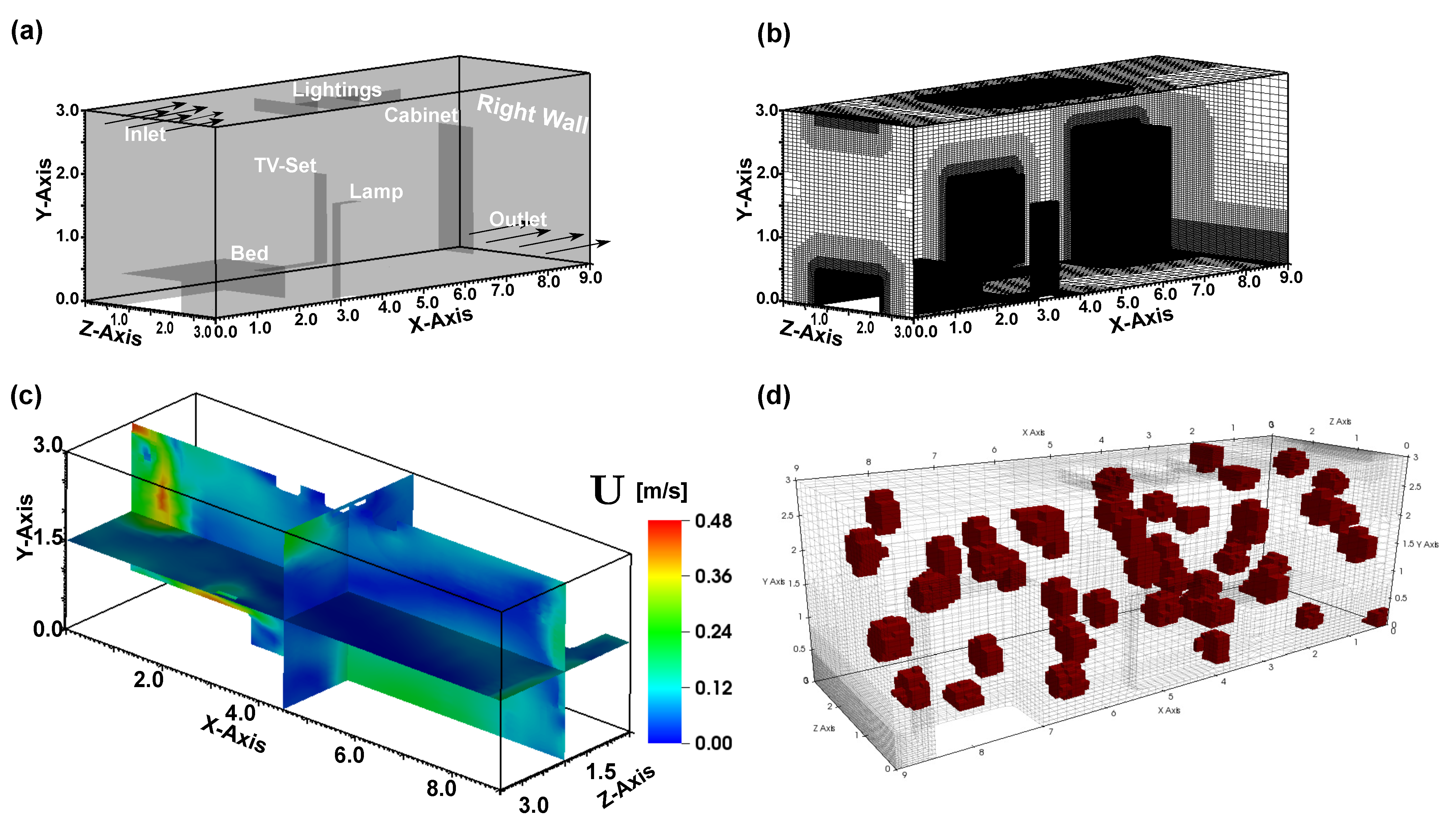
The method is next illustrated for a case with a three-dimensional furnished room. The number of release states is nearly ten times that of the two-dimensional problem. The illustration shows the application of the methodology in a realistic indoor environment and the easy extension of the approach to a relatively complex geometry. Figure 7a shows the three-dimensional furnished room with a bed, TV-set, lamp, lighting, and cabinet represented in the primitive shapes. The room has dimensions 9 m × 3 m × 3 m size with an inlet and outflow to produce a steady vented room. A window is positioned on the right wall with a constant temperature of 302 K. These boundary conditions are used to solve the flow field using the OpenFOAM CFD solver buoyantBoussinesqSimpleFoam. The mesh convergence analysis is carried to ensure the grid independence of the results and 0.6 M cells are used for CFD computation (validation of the used solver and grid independence shown in Appendix A and Appendix B). As described in Section 2.2 the size of the transfer operator is equivalent to the number of states/cells used in the computation of the flow field. We note that the CFD mesh needs to be well resolved to capture the flow features, but the contaminant transport can be reliably simulated on a coarser mesh. We, therefore, interpolate the flow field onto a coarser mesh size of around 70 K cells. The use of CFD mesh would result in a transfer matrix of size . This large matrix will require a lot of memory to store, and subsequent analysis will become infeasible. Therefore, the transfer operator constructed is of size . The optimal sensor algorithm shown in [34] is used to place twelve sensors in the room.
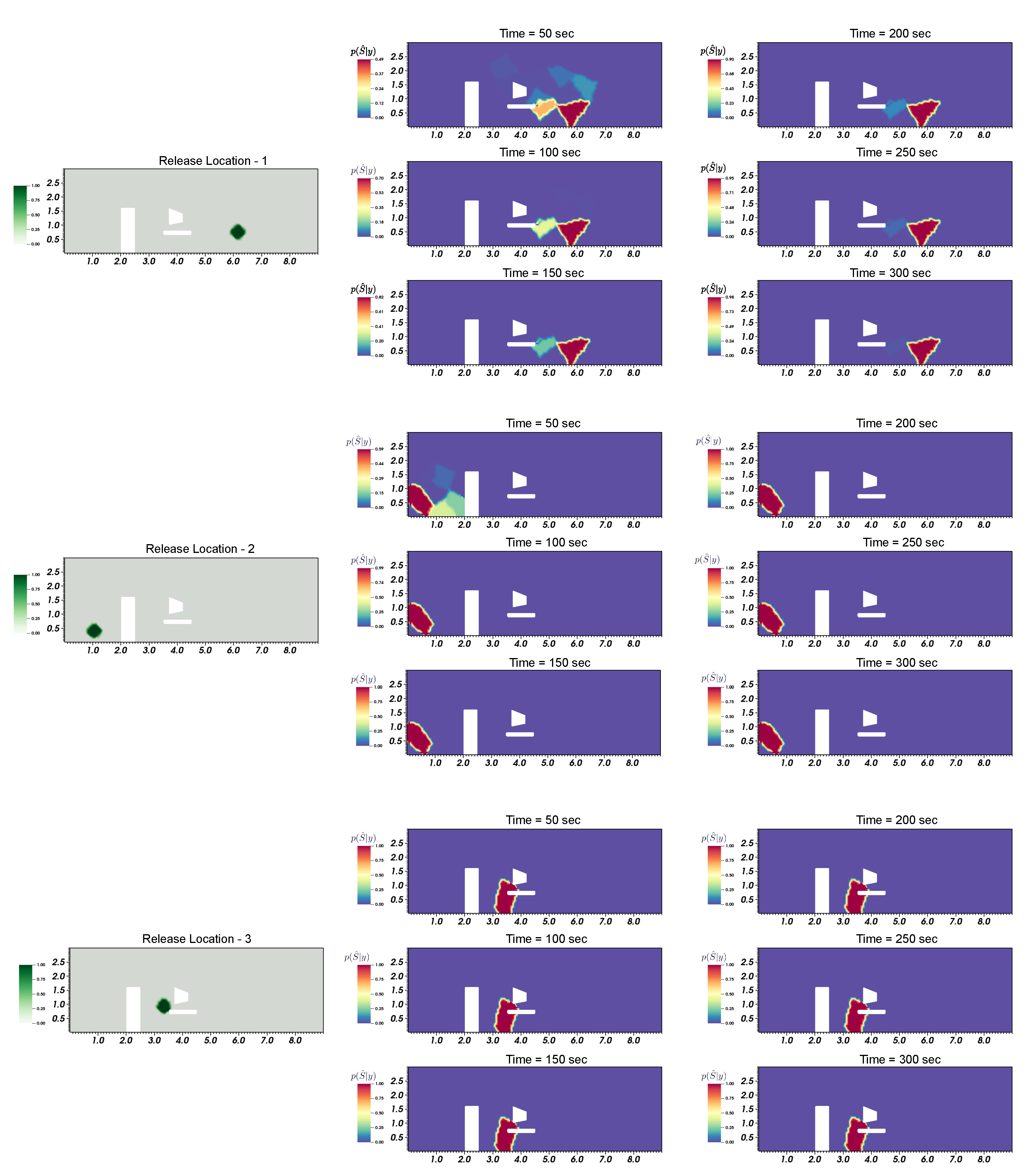
The transfer operator has the evolution time step s. The sensors samples every s, the final simulation time s based on the air change rate of the room. The room is sampled with 50 quasi-random samples in the domain with an epsilon radius of 0.5 m are shown in, Figure 7d, as release locations. For these samples, the model measurement data are computed used for likelihood calculation during real-time Bayesian inference. Three separate random un-sampled release location. We test more than three unknown random release locations. For presentation purposes, we only show three out of them. is simulated to demonstrate the real-time implementation of the approach. The real-time measurements of the sensors are generated with an additional white noise of zero mean and variance of 0.03. Figure 8 shows the posterior map of the release location for the three releases at every sampling time-step. The posteriors are converging to the actual release since we have sufficiently sampled the space to construct the model measurement data. In addition, the result is a posterior distribution of the probable release location. The actual epsilon ball of the release location is not recovered. It can be seen that the posterior closely represent the actual release location in the domain as probable regions.
4. Discussion
The sequential Bayesian inference method in association with the transfer operator approach for simulating the contaminant evolution is developed. The contaminant release locations are identified as a posterior map in the domain. The approach overcomes the real-time implementation limitation posed by traditional Markov Chain Monte Carlo (MCMC) sampling by relying on a Bayes Monte Carlo approach with pre-sampling from the prior distribution of the release locations. The sampling is exhaustive to ensure that the integration in the Bayes formula is accurate. We simulate contaminant releases from these sampled locations and store sensor time-series data. These actual measurements are used for comparing against the real-time streaming data from sensors using the likelihood function. The actual measurements can be generated concurrently as well by simply evolving each release location till the real-time measurement step. The approach is illustrated for both two and three-dimensional building space.
Earlier works in the literature [24,47,50] have reported the use of similar Bayes formulations for source identification but were either based on zonal models or empirical correlations as the forward models. In addition, some reported works rely on steady-state assumptions for estimating contaminant distribution. These assumptions are not well suited for studying the dynamic nature of contaminant evolution in the domain. Therefore, these approaches are usually sub-optimal for real-time implementation and accurately locating release locations. In the present approach, we try to overcome the limitation of the computational complexity of the contaminant transport model via a PF operator approach that results in a simple matrix-vector multiplication for contaminant evolution. The dynamical system setting used here has previously been used for applications including sensor placement under deterministic or stochastic setting [10,35,51,52]. This PF approach provides a unified framework for analysis of building systems during the design/planning phase as well as for risk assessment.
One of the limitations of the present approach is that a good estimate for for the likelihood function is needed. However, the choice of sigma can be improved using prior model measurements under hypothetical release cases, to reduce the error in the prediction. Further, with the use of good computational methods like adaptive sampling, approximate Bayesian computation using sequential Monte Carlo can be performed.
The accidental or intentional release of hazardous compounds (even in minuscule quantities for short periods) can result in lethal and catastrophic consequences. Therefore, a fast, accurate and reliable source identification method is important for containment and speedy evacuation of the occupants. It is important to resolve the smallest to the largest time scales of the contaminant evolution which can be accomplished easily using the PF operator approach. Furthermore, these estimated contaminant locations can easily assist the rescue team in deciding the efficient evacuation strategy and can also be used to controlling the HVAC unit for the building. In addition, for complex imperfect dynamical systems described in [53], the approach could also be leveraged for designing robust control.
5. Conclusions
We present a method for identifying contaminant source location using the PF operator-based transport model coupled with a sequential Bayesian inference formulation. The approach PF based contaminant transport model provides a fast, accurate, and robust method to act as a forward model for contaminant evolution. The approach reduces the computation cost of numerically solving a PDE to simple matrix-vector multiplication. This makes Bayesian inference computationally easy to implement in real-time. The data required for computing the likelihood can be pre-computed. This means that if we have past measurements and some intuition of the release location, pre-computation is possible or the calculations can be made on the fly for multiple sampled release scenario. In the current work, we have shown the use of a quasi-random space-filling sampling approach to sampling the probable release locations in the room and have conducted the likelihood estimate on the fly . For these locations, the constant contaminant release was simulated.
The temporal measurements of the concentrations at the placed sensors in the room the temporal were stored for computing the likelihood in real-time operation. The implementation results are illustrated both in two-dimensional and three-dimensional building problems. We show the results of source identification both in 2D and a 3D problem for three unknown random constant contaminant release scenarios and compute the temporal updated posterior of release location. The results show that the posterior converges to a region within two-three time steps. In the future, we plan to extend the approach for computing various other parameters such as, release rate and implementing the approach for multiple release identification.
Author Contributions
Conceptualization, H.S. and B.G.; methodology, H.S., B.G. and U.V.; software, H.S.; validation, H.S., B.G. and U.V.; formal analysis, H.S. and B.G.; investigation, H.S. and B.G; resources, B.G.; data curation, H.S.; writing—original draft preparation, H.S.; writing—review and editing, H.S., B.G., U.V.; visualization, H.S.; supervision, B.G., U.V.; project administration, B.G.; funding acquisition B.G. and U.V. All authors have read and agreed to the published version of the manuscript.
Funding
UV would like to acknowledge the financial support from the National Science Foundation grants 2031573 and NSF CPS award 1932458. BG acknowledges partial support from NSF 2053760, and NSF 1954556.
Conflicts of Interest
The authors declare no conflict of interest.
Appendix A. Validation of CFD Solvers
The buoyantSimpleFoam of OpenFOAM used for the two-dimensional problem is validated by comparing the solver results with experimental data by Bett et al. [54] for natural convection in the tall cavity. Figure A1a,b shows the comparison of the vertical velocity comparison along the channel width and the temperature profile. The results ensure the solver capability of accurately modeling the heat transfer problem. Therefore the solver is used for the current two-dimensional office problem with multiple heat source.
We validate our numerical solver for three dimensional under iso-thermal setting for by comparing with the experiment by Nielsen et al. [48,55]. Figure A1c,d validated the solver computations for the three dimensional geometry used in the study, by plotting the velocity profile along the X = 1 × H and X = 2 × H for z = 0.5 × W, where W is the width of the room. The profile obtained by the computation matches closely with the experiment results with a slight overshoot on the top wall boundary for X = 1 × H. The rigorous validation of the CFD solver under non-isothermal conditions are already shown by Fontanini et al. [43]. They showed the solver performance against the experimental benchmark problem by Nielsen et al. [56]. The results from the work ensured the use of the solver for the present study.
Figure A1.
(a,b) Vertical velocity profile and temperature profile for the long cavity along X axis as discussed in [54]. (c,d) Normalized velocity profile for the two dimensional model along Y axis for X = 1 × H and X = 2 × H is shown.
Figure A1.
(a,b) Vertical velocity profile and temperature profile for the long cavity along X axis as discussed in [54]. (c,d) Normalized velocity profile for the two dimensional model along Y axis for X = 1 × H and X = 2 × H is shown.

Appendix B. Grid Convergence
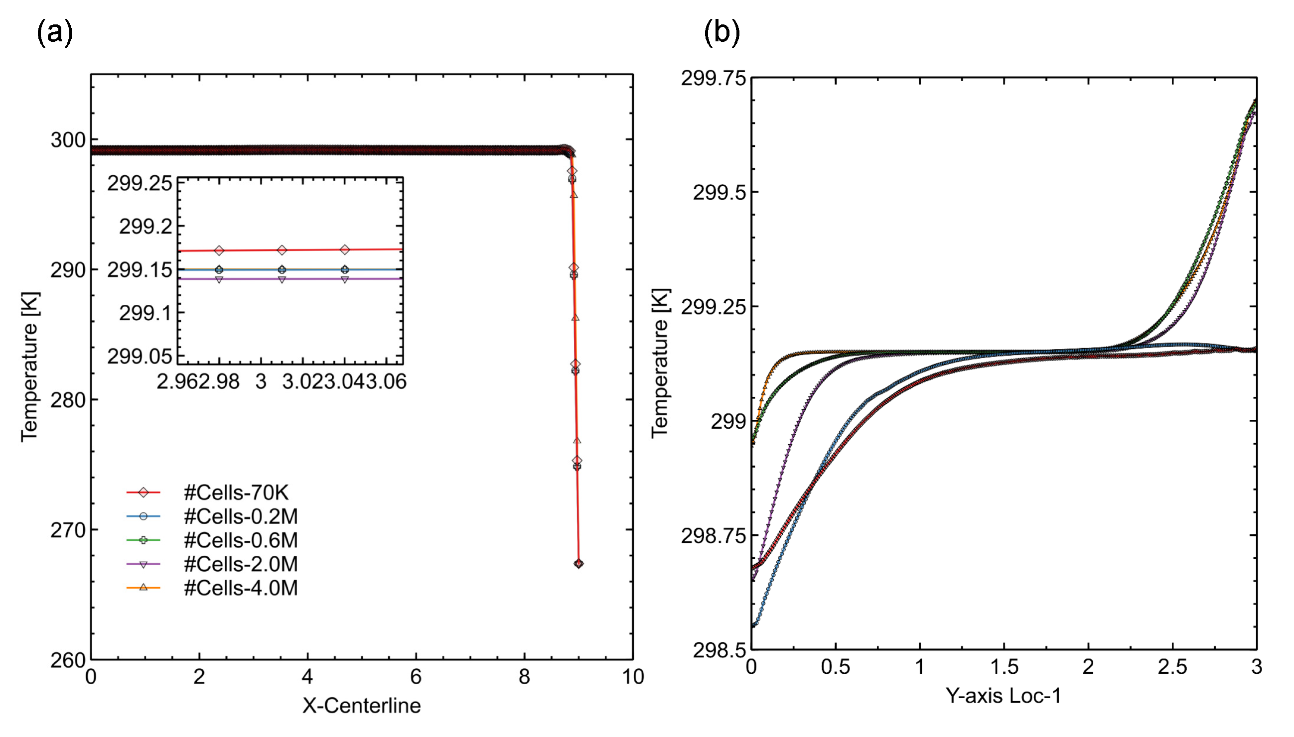
The grid convergence study is performed using the constant right wall temperature of 267 K and an inlet temperature of 300 K for the 3D geometry. The temperature profiles are shown in Figure A2 plotted along the x-axis passing through the room center and along an arbitrary chosen y-axis close to cabinet ((7.5,0,0.5),(7.5,3.0,0.5)) for the 3D geometry (Figure 7). It can be seen that for all the meshes the X-centerline profile closely overlaps each other. While in case of Y-line the difference is mere ±0.2 K between the fine 4.0 M mesh and the chosen 0.6 M mesh. Therefore, all the CFD computations to compute the flow field were carried using 0.6 M mesh.
Figure A2.
Grid independence study for 3D numerical computation: (a) Temperature profile comparison of various grids on x-centerline; (b) temperature profile comparison of various grid along y-axis close to the cabinet in the 3D geometry.
Figure A2.
Grid independence study for 3D numerical computation: (a) Temperature profile comparison of various grids on x-centerline; (b) temperature profile comparison of various grid along y-axis close to the cabinet in the 3D geometry.

References
- EPA/Office of Radiation and Indoor Air. The Inside Story: A Guide to Indoor Air Quality. 2012. Available online: https://www.epa.gov/indoor-air-quality-iaq/inside-story-guide-indoor-air-quality (accessed on 15 September 2021).
- Inglesby, T.V.; O’toole, T.; Henderson, D.A.; Bartlett, J.G.; Ascher, M.S.; Eitzen, E.; Friedlander, A.M.; Gerberding, J.; Hauer, J.; Hughes, J.; et al. Anthrax as a biological weapon, 2002: Updated recommendations for management. JAMA 2002, 287, 2236–2252. [Google Scholar] [CrossRef] [PubMed]
- Pangi, R. Consequence management in the 1995 sarin attacks on the Japanese subway system. Stud. Confl. Terror. 2002, 25, 421–448. [Google Scholar] [CrossRef]
- Moser, M.R.; Bender, T.R.; Margolis, H.S.; Noble, G.R.; Kendal, A.P.; Ritter, D.G. An outbreak of influenza aboard a commercial airliner. Am. J. Epidemiol. 1979, 110, 1–6. [Google Scholar] [CrossRef] [PubMed]
- Olsen, S.J.; Chang, H.L.; Cheung, T.Y.Y.; Tang, A.F.Y.; Fisk, T.L.; Ooi, S.P.L.; Kuo, H.W.; Jiang, D.D.S.; Chen, K.T.; Lando, J.; et al. Transmission of the Severe Acute Respiratory Syndrome on Aircraft. N. Engl. J. Med. 2003, 349, 2416–2422. [Google Scholar] [CrossRef]
- Morawska, L.; Tang, J.W.; Bahnfleth, W.; Bluyssen, P.M.; Boerstra, A.; Buonanno, G.; Cao, J.; Dancer, S.; Floto, A.; Franchimon, F.; et al. How can airborne transmission of COVID-19 indoors be minimised? Environ. Int. 2020, 142, 105832. [Google Scholar] [CrossRef]
- Zhang, R.; Li, Y.; Zhang, A.L.; Wang, Y.; Molina, M.J. Identifying airborne transmission as the dominant route for the spread of COVID-19. Proc. Natl. Acad. Sci. USA 2020, 117, 14857–14863. [Google Scholar] [CrossRef]
- Bloch, A.B.; Orenstein, W.A.; Ewing, W.M.; Spain, W.H.; Mallison, G.F.; Herrmann, K.L.; Hinman, A.R. Measles outbreak in a pediatric practice: Airborne transmission in an office setting. Pediatrics 1985, 75, 676–683. [Google Scholar]
- Menzies, D.; Fanning, A.; Yuan, L.; FitzGerald, J.M. Hospital ventilation and risk for tuberculous infection in Canadian health care workers. Ann. Intern. Med. 2000, 133, 779–789. [Google Scholar] [CrossRef]
- Sharma, H.; Vaidya, U.; Ganapathysubramanian, B. Estimating contaminant distribution from finite sensor data: Perron Frobenious operator and ensemble Kalman Filtering. Build. Environ. 2019, 159, 106148. [Google Scholar] [CrossRef]
- Rao, K.S. Source estimation methods for atmospheric dispersion. Atmos. Environ. 2007, 41, 6964–6973. [Google Scholar]
- Neupauer, R.M.; Wilson, J.L. Adjoint method for obtaining backward-in-time location and travel time probabilities of a conservative groundwater contaminant. Water Resour. Res. 1999, 35, 3389–3398. [Google Scholar] [CrossRef]
- Zhang, T.; Chen, Q. Identification of contaminant sources in enclosed spaces by a single sensor. Indoor Air 2007, 17, 439–449. [Google Scholar] [CrossRef]
- Zhang, T.; Chen, Q. Identification of contaminant sources in enclosed environments by inverse CFD modeling. Indoor Air 2007, 17, 167–177. [Google Scholar] [CrossRef]
- Zhang, T.; Yin, S.; Wang, S. An inverse method based on CFD to quantify the temporal release rate of a continuously released pollutant source. Atmos. Environ. 2013, 77, 62–77. [Google Scholar] [CrossRef]
- Zhang, T.; Zhou, H.; Wang, S. Inverse identification of the release location, temporal rates, and sensor alarming time of an airborne pollutant source. Indoor Air 2015, 25, 415–427. [Google Scholar] [CrossRef]
- Wei, Y.; Zhou, H.; Zhang, T.T.; Wang, S. Inverse identification of multiple temporal sources releasing the same tracer gaseous pollutant. Build. Environ. 2017, 118, 184–195. [Google Scholar] [CrossRef]
- Matsuo, T.; Kondo, A.; Shimadera, H.; Kyuno, T.; Inoue, Y. Estimation of indoor contamination source location by using variational continuous assimilation method. In Building Simulation; Springer: Berlin, Germany, 2015; Volume 8, pp. 443–452. [Google Scholar]
- Matsuo, T.; Shimadera, H.; Kondo, A. Identification of multiple contamination sources using variational continuous assimilation. Build. Environ. 2019, 147, 422–433. [Google Scholar] [CrossRef]
- Vukovic, V.; Tabares-Velasco, P.C.; Srebric, J. Real-time identification of indoor pollutant source positions based on neural network locator of contaminant sources and optimized sensor networks. J. Air Waste Manag. Assoc. 2010, 60, 1034–1048. [Google Scholar] [CrossRef] [Green Version]
- Bastani, A.; Haghighat, F.; Kozinski, J.A. Contaminant source identification within a building: Toward design of immune buildings. Build. Environ. 2012, 51, 320–329. [Google Scholar] [CrossRef] [PubMed]
- Park, Y.J.; Tagade, P.M.; Choi, H.L. Deep gaussian process-based Bayesian inference for contaminant source localization. IEEE Access 2018, 6, 49432–49449. [Google Scholar] [CrossRef]
- Tagade, P.M.; Jeong, B.M.; Choi, H.L. A Gaussian process emulator approach for rapid contaminant characterization with an integrated multizone-CFD model. Build. Environ. 2013, 70, 232–244. [Google Scholar] [CrossRef] [Green Version]
- Sohn, M.D.; Reynolds, P.; Singh, N.; Gadgil, A.J. Rapidly locating and characterizing pollutant releases in buildings. J. Air Waste Manag. Assoc. 2002, 52, 1422–1432. [Google Scholar] [CrossRef]
- Sreedharan, P.; Sohn, M.D.; Nazaroff, W.W.; Gadgil, A.J. Influence of indoor transport and mixing time scales on the performance of sensor systems for characterizing contaminant releases. Atmos. Environ. 2007, 41, 9530–9542. [Google Scholar] [CrossRef] [Green Version]
- Sohn, M.D.; Lorenzetti, D.M. Siting Bio-Samplers in Buildings. Risk Analysis 2007, 27, 877–886. [Google Scholar] [CrossRef] [PubMed]
- Walter, T.; Lorenzetti, D.M.; Sohn, M.D. Siting samplers to minimize expected time to detection. Risk Anal. Int. J. 2012, 32, 2032–2042. [Google Scholar] [CrossRef] [PubMed] [Green Version]
- Sreedharan, P.; Sohn, M.D.; Nazaroff, W.W.; Gadgil, A.J. Towards improved characterization of high-risk releases using heterogeneous indoor sensor systems. Build. Environ. 2011, 46, 438–447. [Google Scholar] [CrossRef] [Green Version]
- Neupauer, R.M. Adjoint sensitivity analysis of contaminant concentrations in water distribution systems. J. Eng. Mech. 2010, 137, 31–39. [Google Scholar] [CrossRef]
- Liu, X.; Zhai, Z.J. Prompt tracking of indoor airborne contaminant source location with probability-based inverse multi-zone modeling. Build. Environ. 2009, 44, 1135–1143. [Google Scholar] [CrossRef]
- Liu, X.; Zhai, Z. Location identification for indoor instantaneous point contaminant source by probability-based inverse Computational Fluid Dynamics modeling. Indoor Air 2007, 18, 2–11. [Google Scholar] [CrossRef] [PubMed]
- Zhai, Z.; Liu, X.; Wang, H.; Li, Y.; Liu, J. Experimental verification of tracking algorithm for dynamically-releasing single indoor contaminant. Build. Simul. 2012, 5, 5–14. [Google Scholar] [CrossRef] [PubMed]
- Wang, H.; Lu, S.; Cheng, J.; Zhai, Z. Inverse modeling of indoor instantaneous airborne contaminant source location with adjoint probability-based method under dynamic airflow field. Build. Environ. 2017, 117, 178–190. [Google Scholar] [CrossRef] [Green Version]
- Fontanini, A.D.; Vaidya, U.; Ganapathysubramanian, B. A methodology for optimal placement of sensors in enclosed environments: A dynamical systems approach. Build. Environ. 2016, 100, 145–161. [Google Scholar] [CrossRef] [Green Version]
- Fontanini, A.D.; Vaidya, U.; Ganapathysubramanian, B. Constructing Markov matrices for real-time transient contaminant transport analysis for indoor environments. Build. Environ. 2015, 94, 68–81. [Google Scholar] [CrossRef] [PubMed] [Green Version]
- Sinha, S.; Vaidya, U.; Rajaram, R. Operator theoretic framework for optimal placement of sensors and actuators for control of nonequilibrium dynamics. J. Math. Anal. Appl. J. Math. Anal. Appl. 2016, 440, 750–772. [Google Scholar] [CrossRef] [Green Version]
- Vaidya, U.; Rajaram, R.; Dasgupta, S. Actuator and sensor placement in linear advection PDE with building system application. J. Math. Anal. Appl. 2012, 394, 213–224. [Google Scholar] [CrossRef] [Green Version]
- Brand, K.P.; Small, M.J. Updating uncertainty in an integrated risk assessment: Conceptual framework and methods. Risk Analysis 1995, 15, 719–729. [Google Scholar] [CrossRef]
- Dilks, D.W.; Canale, R.P.; Meier, P.G. Development of Bayesian Monte Carlo techniques for water quality model uncertainty. Ecol. Model. 1992, 62, 149–162. [Google Scholar] [CrossRef] [Green Version]
- Schmid, P.J. Dynamic mode decomposition of numerical and experimental data. J. Fluid Mech. 2010, 656, 5–28. [Google Scholar] [CrossRef] [Green Version]
- Rowley, C.W.; Mezić, I.; Bagheri, S.; Schlatter, P.; Henningson, D.S. Spectral analysis of nonlinear flows. J. Fluid Mech. 2009, 641, 115–127. [Google Scholar] [CrossRef] [Green Version]
- Mezić, I. Spectral properties of dynamical systems, model reduction and decompositions. Nonlinear Dyn. 2005, 41, 309–325. [Google Scholar] [CrossRef]
- Fontanini, A.; Vaidya, U.; Passalacqua, A.; Ganapathysubramanian, B. Contaminant transport at large Courant numbers using Markov matrices. Build. Environ. 2017, 112, 1–16. [Google Scholar] [CrossRef]
- Sinha, S.; Huang, B.; Vaidya, U. Robust Approximation of Koopman Operator and Prediction in Random Dynamical Systems. In Proceedings of the 2018 Annual American Control Conference (ACC), Milwaukee, WI, USA, 27–29 June 2018; pp. 5491–5496. [Google Scholar]
- Williams, M.O.; Kevrekidis, I.G.; Rowley, C.W. A data–driven approximation of the koopman operator: Extending dynamic mode decomposition. J. Nonlinear Sci. 2015, 25, 1307–1346. [Google Scholar] [CrossRef] [Green Version]
- Gelman, A.; Stern, H.S.; Carlin, J.B.; Dunson, D.B.; Vehtari, A.; Rubin, D.B. Bayesian Data Analysis; Chapman and Hall/CRC: London, UK, 2013. [Google Scholar]
- Michael Sohn, B.D.; Member, A.; Small, M.J.; Pantazidou, M. Reducing uncertainty in site characterization using Bayes Monte Carlo methods. J. Environ. Eng. 2000, 126, 893. [Google Scholar] [CrossRef]
- Nielsen, P.V. Specification of Two Dimensional Test Case; Technical Report; Aalborg University: Aalborg, Denmark, 1990. [Google Scholar]
- Jasak, H.; Jemcov, A.; Tukovi, Z. OpenFOAM: A C++ Library for Complex Physics Simulations. In International Workshop on Coupled Methods in Numerical Dynamics IUC; IUC Dubrovnik Croatia: Dubrovnik, Croatia, 2007. [Google Scholar]
- Zeng, L.; Gao, J.; Du, B.; Zhang, R.; Zhang, X. Probability-based inverse characterization of the instantaneous pollutant source within a ventilation system. Build. Environ. 2018, 143, 378–389. [Google Scholar] [CrossRef]
- Sharma, H.; Fontanini, A.D.; Vaidya, U.; Ganapathysubramanian, B. Transfer Operator Theoretic Framework for Monitoring Building Indoor Environment in Uncertain Operating Conditions. In Proceedings of the 2018 Annual American Control Conference (ACC), Milwaukee, WI, USA, 27–29 June 2018; pp. 6790–6797. [Google Scholar]
- Sharma, H.; Vaidya, U.; Ganapathysubramanian, B. A transfer operator methodology for optimal sensor placement accounting for uncertainty. Build. Environ. 2019, 155, 334–349. [Google Scholar] [CrossRef] [Green Version]
- Bucolo, M.; Buscarino, A.; Famoso, C.; Fortuna, L.; Frasca, M. Control of imperfect dynamical systems. Nonlinear Dyn. 2019, 98, 2989–2999. [Google Scholar] [CrossRef]
- Betts, P.; Bokhari, I. Experiments on turbulent natural convection in an enclosed tall cavity. Int. J. Heat Fluid Flow 2000, 21, 675–683. [Google Scholar] [CrossRef]
- Nielsen, P.V.; Restivo, A.; Whitelaw, J.H. The Velocity Characteristics of Ventilated Rooms. J. Fluids Eng. 1978, 100, 291–298. [Google Scholar] [CrossRef]
- Nielsen, P.V.; Murakami, S.; Kato, S.; Topp, C.; Yang, J.H. Benchmark tests for a computer simulated person. In Indoor Environmental Engineering; Aalborg University: Aalbrog, Denmark, 2003. [Google Scholar]
Figure 1.
For the given velocity field (a,b) Shows the contaminant transport using the scalar transport Equation (1) (c,d) Shows the discrete PF-operator based scalar transport.
Figure 1.
For the given velocity field (a,b) Shows the contaminant transport using the scalar transport Equation (1) (c,d) Shows the discrete PF-operator based scalar transport.

Figure 2.
Flow chart of complete real-time Bayesian inference based on PF operator approach.

Figure 3.
(a) Geometry and boundary conditions are used for computing the velocity flow field. (b) The velocity magnitude computed and used for computing the transfer operator.
Figure 3.
(a) Geometry and boundary conditions are used for computing the velocity flow field. (b) The velocity magnitude computed and used for computing the transfer operator.

Figure 4.
(a) Initial condition for the concentration. (b) Numerically solved PDE transport for contaminant evolution at time 50 s. (c) Contaminant evolution using the transfer operator at time 50 s. (d) Contaminant concentration comparison between PDE and Markov model along center X and Y axis of the computational domain.

Figure 5.
(a) The 2D computational domain with the boundary conditions is used for calculating the flow field in the domain. (b) The CFD computational mesh is used for computing the flow field and the transfer operator. (c) The computed velocity magnitude inside the room. (d) Sampled 50 release locations with radius 0.25 m, used in the likelihood calculation during Bayesian inference.

Figure 6.
Bayesian inference is posterior for three random releases at every observation time step.

Figure 7.
(a) The geometry used in the 3D room is used for the construction of the Markov matrix. (b) The computational mesh is used for performing the CFD for computing the flow field in the room. (c) The computed velocity is shown on the midplane of the room. (d) The sampled release locations which are going to be used for computing the likelihood in the Bayesian inference.

Figure 8.
Bayesian inference Iso-Contours of the posterior for three random releases at every observation time step in the three-dimensional room. The region of the release are shown in red color for each release.
Figure 8.
Bayesian inference Iso-Contours of the posterior for three random releases at every observation time step in the three-dimensional room. The region of the release are shown in red color for each release.

Publisher’s Note: MDPI stays neutral with regard to jurisdictional claims in published maps and institutional affiliations. |
© 2021 by the authors. Licensee MDPI, Basel, Switzerland. This article is an open access article distributed under the terms and conditions of the Creative Commons Attribution (CC BY) license (https://creativecommons.org/licenses/by/4.0/).
Share and Cite
MDPI and ACS Style
Sharma, H.; Vaidya, U.; Ganapathysubramanian, B. Contaminant Source Identification from Finite Sensor Data: Perron–Frobenius Operator and Bayesian Inference. Energies 2021, 14, 6729. https://doi.org/10.3390/en14206729
AMA Style
Sharma H, Vaidya U, Ganapathysubramanian B. Contaminant Source Identification from Finite Sensor Data: Perron–Frobenius Operator and Bayesian Inference. Energies. 2021; 14(20):6729. https://doi.org/10.3390/en14206729
Chicago/Turabian StyleSharma, Himanshu, Umesh Vaidya, and Baskar Ganapathysubramanian. 2021. "Contaminant Source Identification from Finite Sensor Data: Perron–Frobenius Operator and Bayesian Inference" Energies 14, no. 20: 6729. https://doi.org/10.3390/en14206729
Note that from the first issue of 2016, this journal uses article numbers instead of page numbers. See further details here.