Article

Atmospheric Stability Effects on Offshore and Coastal Wind Resource Characteristics in South Korea for Developing Offshore Wind Farms

1
Interdisciplinary Program of Renewable Energy Engineering, Mokpo National University, Mokpo 58554, Korea
2
Wind Energy Research Center, Energy Valley Industry-University Convergence Agency, Naju 58277, Korea
3
Wind Energy Research Team, Korea Institute of Energy Research, Jeju 63357, Korea
4
Wind & Marine Energy Department, Green Energy Institute, Mokpo 58656, Korea
5
Renewable Energy Group, KEPCO Research Institute, Daejeon 34056, Korea
6
Department of Electrical and Control Engineering, Mokpo National University, Mokpo 58554, Korea
*
Author to whom correspondence should be addressed.
Energies 2022, 15(4), 1305; https://doi.org/10.3390/en15041305
Submission received: 30 December 2021 / Revised: 29 January 2022 / Accepted: 10 February 2022 / Published: 11 February 2022

Abstract

:
South Korea is surrounded by the sea on three sides. The characteristics of offshore wind resources vary from region to region due to the influence of the distribution of the coastline and differences in roughness length and atmospheric stability between the coast and the sea. In particular, turbulent gusts and low-level wind shear occurring near the hub height of the wind turbine within the atmospheric boundary layer have a significant effect on the load of wind turbines. These severe weather phenomena are closely related to atmospheric stability. Therefore, the objective of this study is to determine differences in wind resource characteristics in the South Korean offshore and coast in relation to variations in atmospheric stability using observation data from the HeMOSU-1 meteorological tower in the West Sea and the Boseong meteorological observation tower on the southern coast. On the southern coast, changes in sea and land breezes are observed throughout diurnal and nocturnal periods, with an atmospheric stability distribution similar to that of land, which is unstable during the day and becomes more stable at night. On the other hand, the stable ratio continues to dominate in the west offshore. In the case of coastal areas, low-level wind shear occasionally occurs near the general wind turbine hub height approximately over 100 m due to the influence of winds from the sea. This study shows that when constructing an offshore wind farm, it is necessary to first analyze the characteristics of local coastal and offshore wind resources for more efficient and safe wind farm construction and operation.

Graphical Abstract

1. Introduction

Interest in eco-friendly renewable energy sources based on the Korean Green New Deal, 2050 carbon zero, and renewable energy 3020 policies is continuously increasing [1]. In particular, in South Korea, which is surrounded by the sea on three sides, offshore wind energy is attracting attention as a major national power source for the next generation, and the industrial market is also rapidly expanding [2]. This is an energy flow in line with the trend of using renewable energy as the top-priority power source in the national power mix. Wind energy is in the spotlight as a sustainable, eco-friendly energy type that will play the most important role in achieving the goals of the RE100 and the Paris Agreement on Climate Change.
Prior to the implementation of the onshore/offshore wind farm project, it is decided whether to proceed with the project by analyzing the wind resources and calculating the expected annual energy production (AEP) based on the actual wind observation data [3]. In general, third-party certification companies perform this analysis, and the report includes information related to wind shear and turbulence intensity [4,5]. However, it only introduces the numerical values and does not specify the rationale for why the wind shear and turbulence intensity in the area show such values.
In particular, it is difficult to characterize and predict wind resources for coastal areas by the West and South Seas because of the shallow water depth and complex distribution of coastlines with many islands [6,7,8,9]. This remains a major issue as most offshore wind energy projects in South Korea are concentrated in the West and South Seas.
It has been shown that the diurnal change in turbulence is 20% larger than that of other regions due to interactions among the atmosphere, land, and ocean in areas with a complex coastal topography [10], implying that large turbulent gusts can be generated by surface-sensible heat fluxes and the growth of turbulence kinetic energy (TKE) during the transition from day to night.
In general, it is difficult to accurately calculate wind resources because the wind in the lower part of the atmospheric boundary layer is generated by the simultaneous action of mechanical forcing due to surface friction and thermal forcing involving the heat balance due to surface heating [11,12]. In particular, in the case of coastal areas, a large amount of water vapor is distributed in the atmosphere and the change in atmospheric stability is relatively larger than that of land due to the difference in heat balance between the ocean and inland [13]. In addition, South Korea has a lot of mountainous terrain and a complex coastline, but not a lot of flat lands compared to its total area. Thus, the wind direction fluctuates widely in South Korea. Therefore, since the horizontal/vertical wind direction fluctuates greatly, a lot of expertise is required to predict the AEP of offshore wind farms and secure the stability of the structure. In order to accurately predict the amount of power generation according to the electric power demand and to ensure the stability of the offshore wind turbine, an atmospheric stability analysis closely related to the wind should be performed [14,15,16]. During the diurnal change, atmospheric stability appears stable or unstable in addition to the neutral state. Therefore, the manufacturer’s wind turbine power curve (manufacture power curve, MPC), assuming atmospheric stability in a neutral state, has no choice but to show a difference from the power curve of the wind turbine installed at the actual site [16,17], and this difference leads to errors in the AEP calculation. The International Electrotechnical Commission (IEC61400-12-1) recognizes that the atmospheric stability characteristics of each site can have a significant impact on wind speed measurement and the actual power output performance of wind turbines [18]. However, the atmosphere is still assumed to be in a neutral state on several reports and software. Therefore, in order to reduce the prediction error in the AEP calculation process, an accurate power curve of the wind turbine according to external environmental conditions, especially atmospheric conditions, is required [12,19]. Atmospheric conditions include turbulence intensity, wind shear, and heat flux, all of which depend largely on atmospheric stability. Therefore, analysis of atmospheric stability is essential [13]. According to a previous study, thermal forcing based on humidity and temperature should be considered before predicting offshore and coastal vertical shear because winds at each vertical layer analyzed from the meteorological observation tower located on the offshore show rapid changes according to atmospheric stability [20]. Moreover, it has been suggested that the difference between sea surface temperature and air temperature should be analyzed because atmospheric stability and baroclinicity play an important role in offshore wind [21,22].
Since the energy generated by the wind turbine is mostly dependent on wind speed, it can be greatly influenced by changes in the daily wind speed. This change in wind speed may vary depending on atmospheric stability, because the atmospheric boundary layer does not exhibit the property of a steady state with time [23,24]. Therefore, the wind power generation has variability according to the heat flux and vertical wind speed change by height according to atmospheric stability. In particular, in the case of onshore wind farms close to the coast, the change in atmospheric stability is also large because the daily wind speed and direction change frequently and the temperature change is large due to the influence of the land–sea breeze compared to the inland [25,26,27,28]. The difference in wind speed by height according to the atmospheric stability affects the wake diffusion of the wind turbine and the power generation, which can also influence the future power supply plan and revenue [29,30,31,32,33]. Studies on the effect of atmospheric stability on wind energy are being actively conducted abroad, but not many studies are being conducted in South Korea.
As mentioned above, changes in atmospheric stability tend to be larger on the coast than on land. The interrelationship between the atmosphere and the ocean can induce changes in the characteristics of each system, thus playing a role in the transition from local meteorological phenomena to global climate change in the long term. Therefore, the importance of wind characteristics research in coastal areas has been highlighted. Related studies are being conducted in various fields.
In this study, wind resource conditions at coastal and offshore areas were compared and analyzed using data from meteorological observation towers located at the Boseong Global Standard Meteorological Observation site and the West Sea area in the Republic of Korea. In order to analyze atmospheric stability, which is closely related to the coastal and offshore winds, a stability classification method according to the Richardson number and wind shear, turbulence kinetic energy (TKE), and Monin–Obukhov length was selected to investigate the relationship of atmospheric stability with wind resources.
Atmospheric stability greatly affects not only the wind power generation but also the stability of structures. Rather than focusing on the economic feasibility of the project, it was decided to proceed with this study because it is believed that detailed meteorological research in the area where the project is to be carried out should be performed prior to the preliminary feasibility study.

2. Data and Methods

Meteorological mast observation data were used to compare the characteristics of wind resource conditions in the West Sea adjacent to the land and in the southern sea coast (Figure 1). Both are meteorological masts operated by public institutions (Korea Electric Power Research Institute, National Institute of Meteorological Sciences) for research purposes. Analysis was performed with consent to a request to use them only for non-profit research purposes. Information on each meteorological mast and observation data are shown as follows (Table 1) (Figure 2).

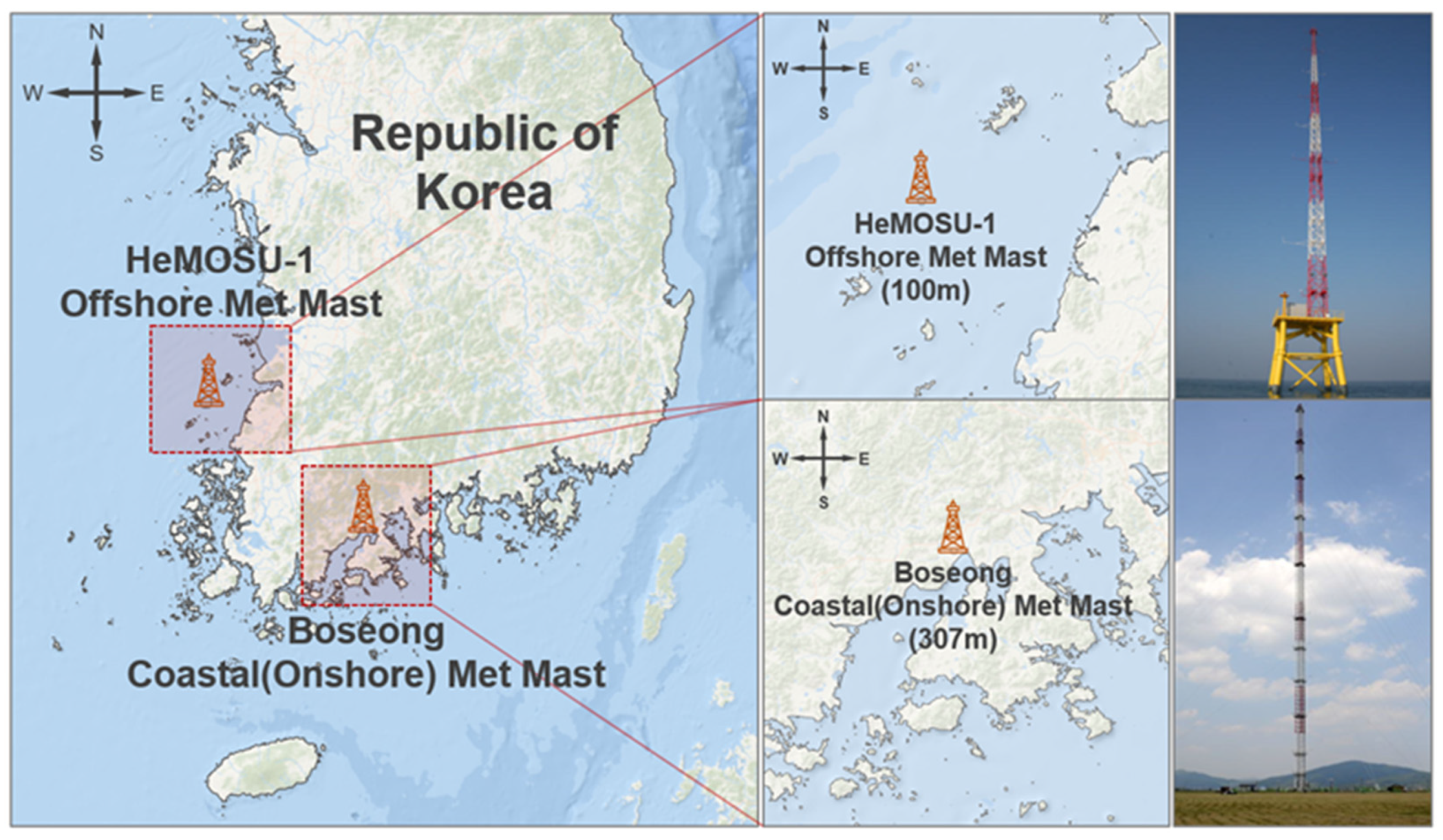
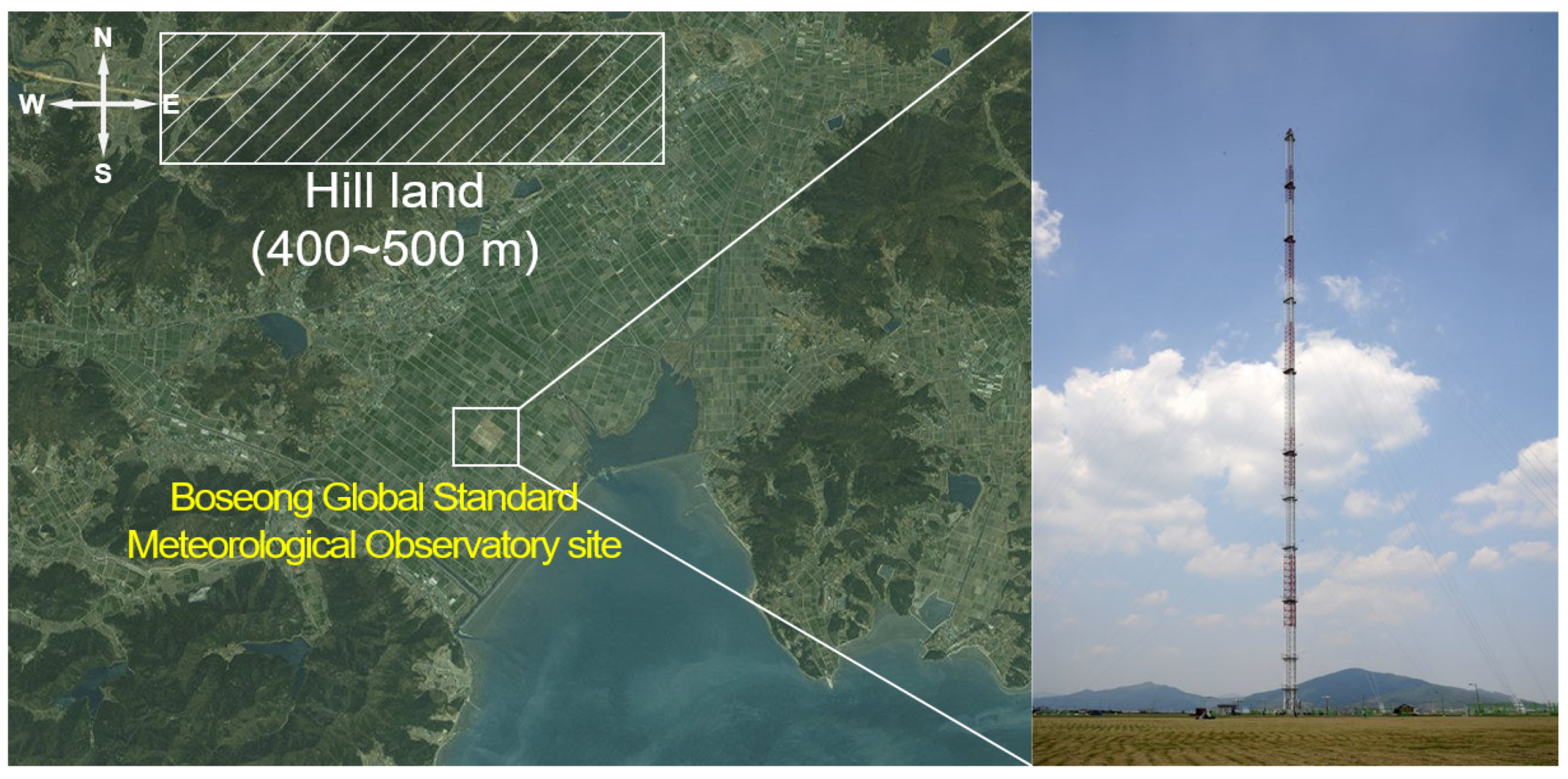
2.1. Boseong Onshore Meteorological Mast

The first meteorological mast is the comprehensive meteorological observation mast in Boseong, Jeollanam-do. A comprehensive meteorological observatory was built to establish a foundation for performing the role of the atmospheric boundary layer characteristic research test bed designated by the World Meteorological Organization (WMO) [34]. The Boseong meteorological mast is installed on homogeneous flat land (Figure 3). It is suitable for local micro-meteorological experiments. It can be used to conduct research on coastal boundary layer structures, typhoons, coastal fog generation, and coastal gusts. It is also the second-tallest meteorological observatory in Asia, with a maximum height of 307 m. Observations are made from a total of 11 altitudes from the ground. Wind speed, wind direction, air temperature, relative humidity, atmospheric pressure, radiation, CO2 · H2O concentration, etc., are observed. Momentum flux, sensible and latent heat flux, friction velocity, and air density are then calculated (Table 2).
The Boseong meteorological mast was built on a reclaimed land. It is adjacent to the coast at a distance of 1.5 km to the southeast and a hilly area at an altitude of 400 to 500 m separated about 5 km to the northwest. Therefore, site conditions are being established to simultaneously analyze the characteristics of the topography and meteorological factors, as well as ocean and meteorological factors. The Boseong meteorological mast is the only and the first in South Korea to produce data on the vertical distribution of high-rise turbulence characteristics. Thus, it has large advantages in that it can also be used for the prediction and diagnosis of local climate change phenomena based on an increased understanding of the atmospheric boundary layer in coastal areas [35]. In this study, data on wind direction, wind speed, friction velocity (u*), air temperature, and sensible heat flux of 10 m, 60 m, 140 m, and 300 m per 10 min from 1 January 2016 to 31 December 2016 were used for the analysis.

2.2. HeMOSU-1 Offshore Meteorological Mast

HErald of Meteorological and Oceanographic Special Unit-1 (HeMOSU-1) is the first offshore meteorological mast to support the development of large-scale offshore wind farms in South Korea. It was installed in February 2011 at 100 m height above mean sea level and 35 km southwest of Gyeokpo Port with support from the government. The meteorological mast has oceanographic observation devices (such as tides, tidal currents, waves, etc.), structural measurement devices that measure the verticality and stress of structures, and meteorological measurement devices that measure wind direction, wind speed, air temperature, air pressure, relative humidity, and precipitation (Table 3). It also consists of a device that stores and transmits these signals. Through this meteorological mast, it is possible to overcome the limitations of reanalysis data or numerical weather prediction model data used in an offshore wind farm project. It is also possible to provide precise measured data that can be directly used in the development of projects [36,37].

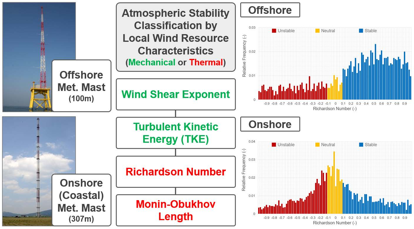
2.3. Atmospheric Stability Index

Atmospheric stability is an important factor used to define atmospheric turbulence or to describe the magnitude of atmospheric diffusion [13]. It refers to the degree to which the atmosphere in a state of mechanical equilibrium is slightly disturbed to return to its original state or the state of the atmosphere is likely to change significantly. Atmospheric stability can be classified into three stages: unstable, neutral, and stable. Atmospheric stability can be broadly classified as mechanical stability and thermal stability. A typical classification method of mechanical atmospheric stability is the vertical wind shear coefficient, which is a principle that determines the degree of flow and diffusion by the transfer of momentum according to the difference in wind speed for each height in the z-direction [14]. Thermal stability such as Richardson number and Monin–Obukhov length not only considers the difference in momentum due to wind speed, but also considers the thermal motion effect due to temperature and heat flux. Table 4 shows atmospheric stability classification criteria and representative meteorological phenomena [19,31,38].
In this study, the characteristics of wind resources according to the atmospheric stability the offshore and coast were analyzed through the Richardson number and wind shear coefficient. Since sensible heat flux and vertical wind speed are only observed at the Boseong meteorological mast, additional atmospheric stability analysis was also conducted along the coast of Boseong according to the Monin–Obukhov length and turbulence kinetic energy (TKE).

2.3.1. Wind Shear Coefficient

The power law describes a functional relationship between two numbers in which one number is theoretically expressed as a power of the other. When the atmospheric stability is near-neutral, the vertical wind speed distribution in which the wind speed constantly increases according to the height even in the lower boundary layer of the atmosphere will appear so that the power law can be applied [39,40]. The wind shear coefficient (α) or power law exponent calculated from this is a correction factor that follows the ground state around the observation point, as shown in Equation (1):
U U r = ( Z Z r ) α
Here, Z [m] is the target height, Zr [m] is the reference height, U [ms−1] is the wind speed at the target height, and Ur [ms−1] is the wind speed at the reference height. Wind shear coefficients can be calculated if wind resource measurements for at least two heights are available by fitting wind speed data with Equation (2):
α = ln ( U ) ln ( U r ) ln ( Z ) ln ( Z r )

2.3.2. Richardson Number

The relative importance of turbulence produced by thermal and mechanical convection can be determined by the Richardson number. When defining the Richardson number, it is convenient to first define the stability parameter S (Equation (3)). The term S is proportional to the rate at which the stable state suppresses turbulence. The concepts of gravitational constant (g, 9.81 m/s2) and potential temperature (θ) are introduced. The potential temperature is defined as the temperature at which a dry air mass at a certain height is adiabatically moved to an 1000 hpa height. An increase in potential temperature by height means that the atmosphere is stable. Turbulence is also created by mechanical convection at a rate proportional to (∂ū/∂z)2. The Richardson number is the ratio of these two processes.
The Richardson number is an indicator of both turbulence and stability. A very negative Richardson number indicates that convection prevails and winds are weak, with a strong vertical motion characteristic of an unstable atmosphere. As the mechanical turbulence increases, the Richardson number approaches zero, with neutral stability (∂θ/∂z = 0). Finally, when the Richardson number becomes positive, vertical mixing stops and the atmosphere stably stratifies, resulting in mechanical turbulence [29,41].
S = g T ( Δ θ Δ Z )
θ = T ( p 0 p ) 0.286
Ri = S ( u ¯ / Z ) 2 = g T ( θ / Z ) ( u ¯ / Z ) 2 = g T 0 ( / Z ) [ θ 0 + θ 1 ] [ ( / Z ) ( u 0 + u 1 ) ] 2

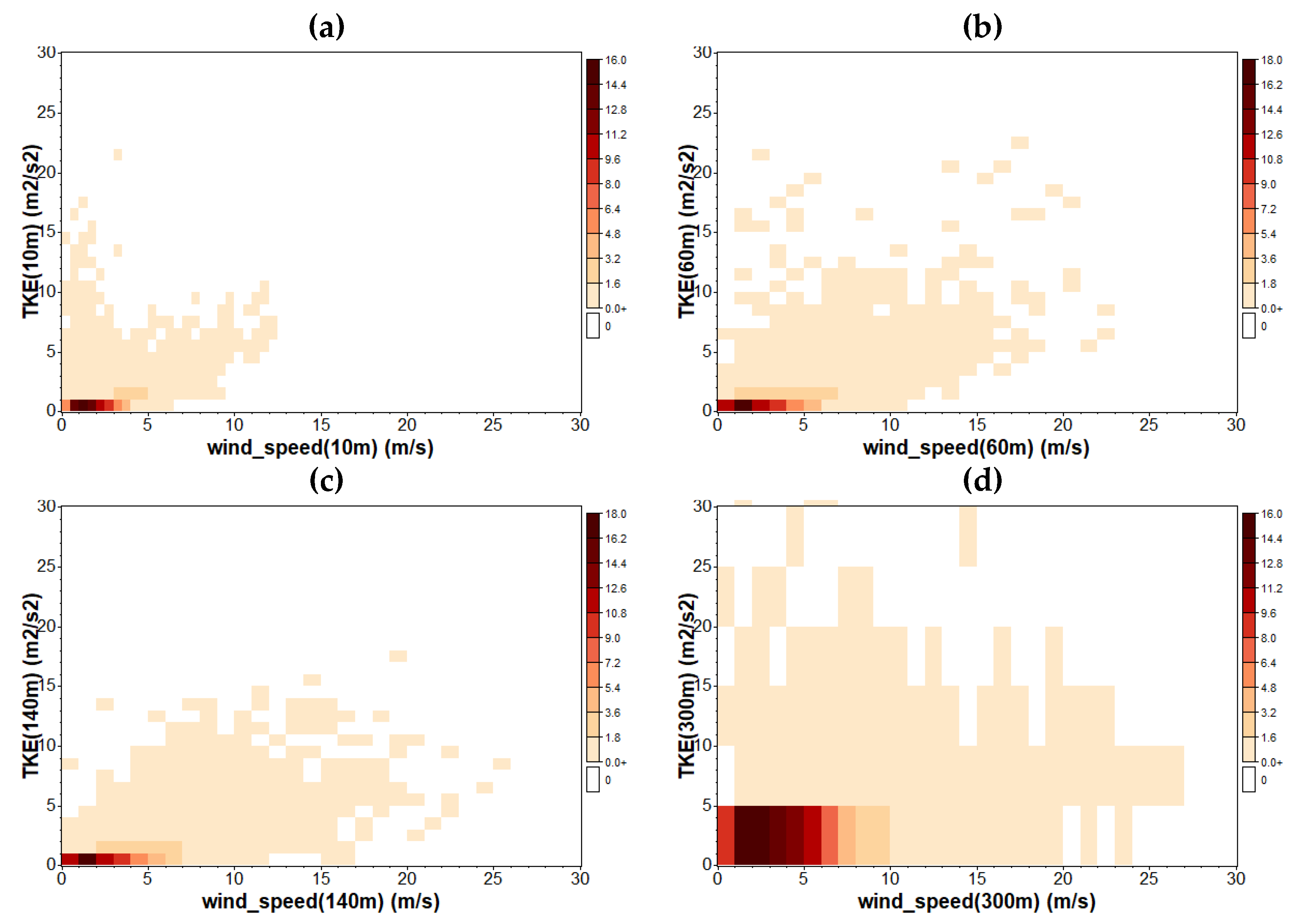
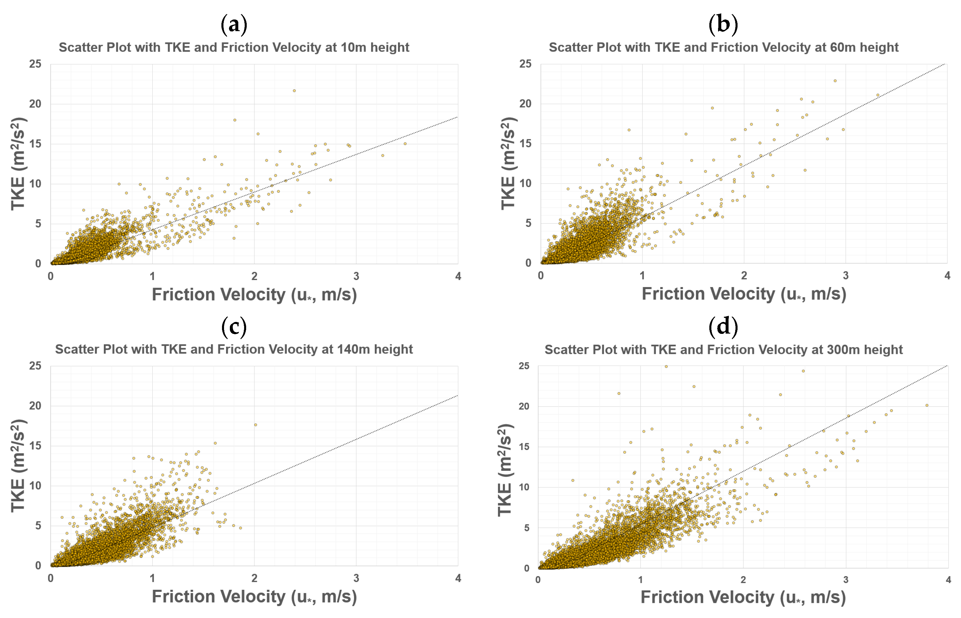
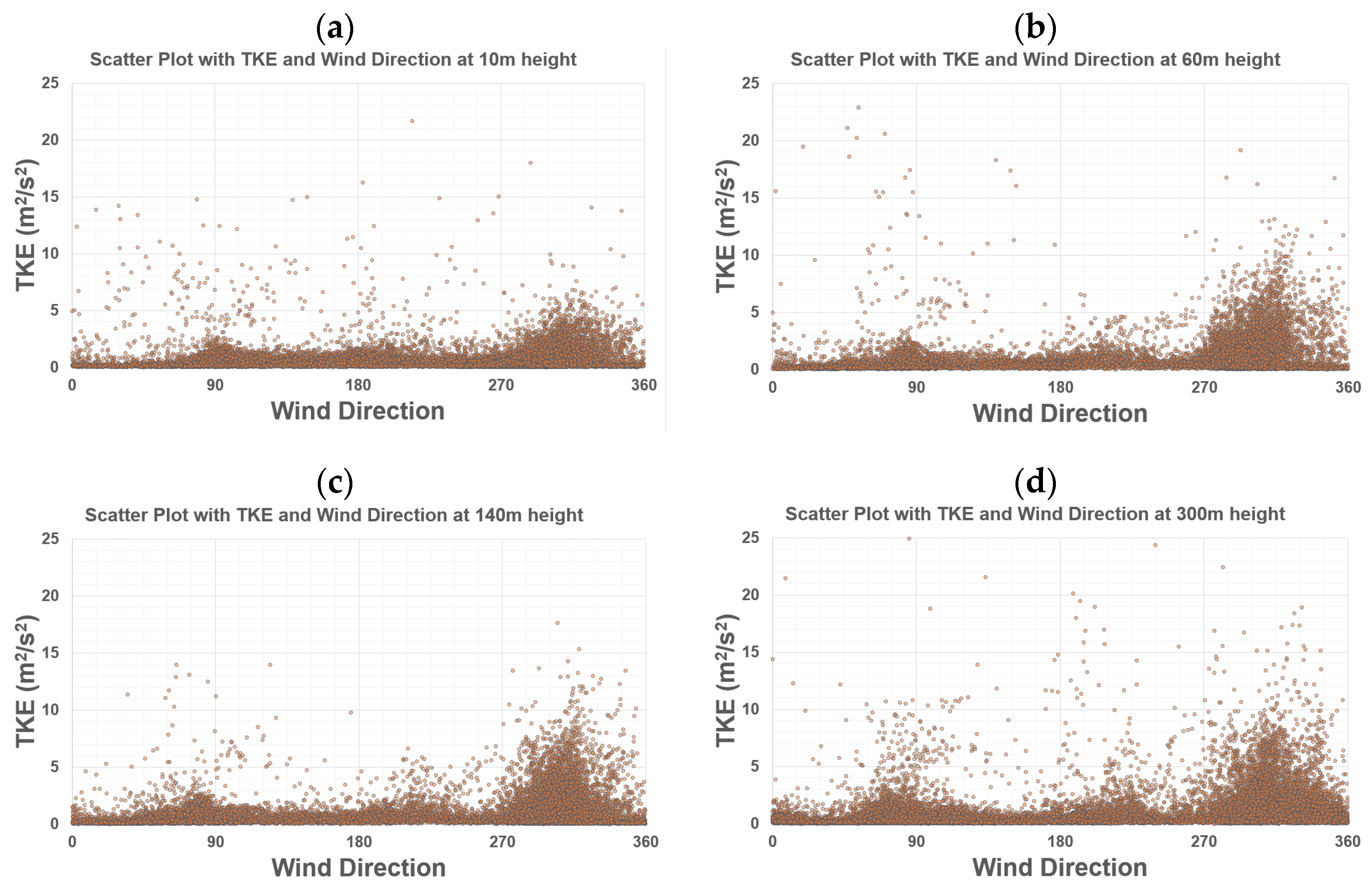
2.3.3. Turbulence Kinetic Energy (TKE)

Wind resource parameters have important effects on wind turbine performance and load. Turbulence measurements are generally performed using instruments placed within the flow, such as cup anemometers, sonic anemometers, and LiDARs. Another detail is that IEC 61400-12-1 requires the horizontal/vertical component of the wind resource to be measured so that the strength of turbulence can be analyzed from the velocity of the horizontal/vertical component [42]. Turbulence kinetic energy explains the generation, maintenance, and dissipation of turbulence. TKE can be obtained by the Reynolds average of the instantaneous kinetic energy per unit mass for turbulence. TKE is a measure of the strength of turbulence. It shows that large-scale turbulence eddies can supply energy to small-scale turbulence eddies. When small-scale eddies cannot be supplied with energy, they disappear due to viscosity on the land surface, as shown in Equations (6) and (7):
TKE = 1 2 ( u ¯ 2 + v ¯ 2 + w ¯ 2 ) = 1 2 ( σ u 2 + σ v 2 + σ w 2 )
k t + u ¯ j k x j = 1 ρ 0 u ι p ¯ x i 1 2 u ȷ u ȷ u ι ¯ x i + ν 2 k x j 2 u ι u ȷ ¯ u ι ¯ x j ν u ι x ȷ u ι x ȷ ¯ g ρ 0 ρ u ι ¯ δ i 3

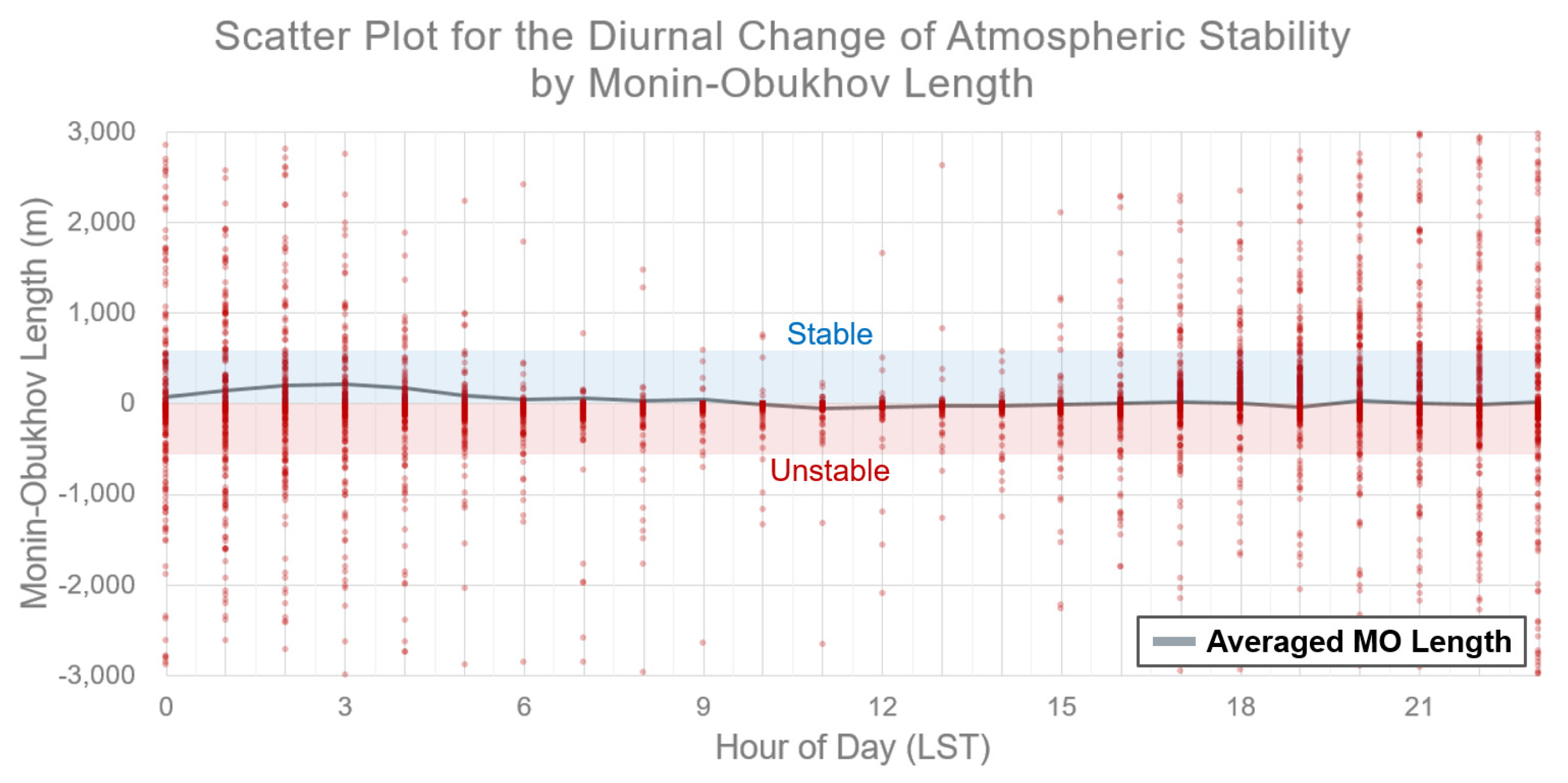
2.3.4. Monin–Obukhov Length

The Monin–Obukhov (MO) length is a similarity theory that states that the turbulent flow characteristics and averaged flow of a fluid depend only on four independent variables: friction velocity, height, surface heat flux, and buoyancy in a horizontally homogeneous surface layer. It is an index of atmospheric stability indicating the degree of dominance of buoyancy over the shear effect. The MO similarity theory is basically organized under five hypotheses [13,43]:
  • The flow is horizontally homogeneous and quasi-stagnate;
  • The momentum and turbulent flux of heat is constant with height;
  • Molecular exchange is not as important as turbulent exchange;
  • The Coriolis effect is neglected in the surface layer;
  • Effects of surface roughness, boundary layer height, and geostrophic winds are all explained by T 0 / ρ .
L = u 3 k g T 0 w T ¯
u 2 = [ u w ¯ 2 + v w ¯ 2 ] 2
In the above equation, u* means friction velocity, g is the gravitational constant (9.81 ms−2), k is the von Karman constant (0.4), T0 is the surface temperature, and w T ¯ is the sensible heat flux data.
Φ m ( ζ ) = k z u u ¯ z
Φ h ( ζ ) = k z u θ ¯ z
u ( z ) = u k [ ln ( z / z 0 ) Ψ m ( z / L ) ]
Ψ m ( z / L ) = 5 · z / L
Ψ m ( z / L ) = 2 · ln [ ( 1 + x ) 2 ] + ln [ ( 1 + x 2 ) 2 ] 2 · t a n 1 ( x ) + π / 2
x = [ 1 ( 16 · z / L ) ] 1 / 4
Ψ m ( z / L ) = 0
In Equations (10) and (11), ζ means z/L. When the value of L is larger than that of z, the shear effect is large. This means that the shear is more important than the buoyancy force because the friction effect is large in the lowest layer (land surface). Conversely, when z is larger than L, it means that the buoyancy effect is greater than the shear in the upper surface or Ekman layer.
Equation (12) can be used to obtain the wind speed at various heights. It is the wind speed value to which the stability parameter Monin–Obukhov length (MO length) corresponds. The last term in Equation (12) is dependent on the atmospheric stability. Equations (13), (14) and (16) are applied according to the stable, unstable, and neutral state of the atmosphere, respectively. This is because changes in momentum and heat flux according to atmospheric stability can determine the shape of the vertical distribution of the wind resource.

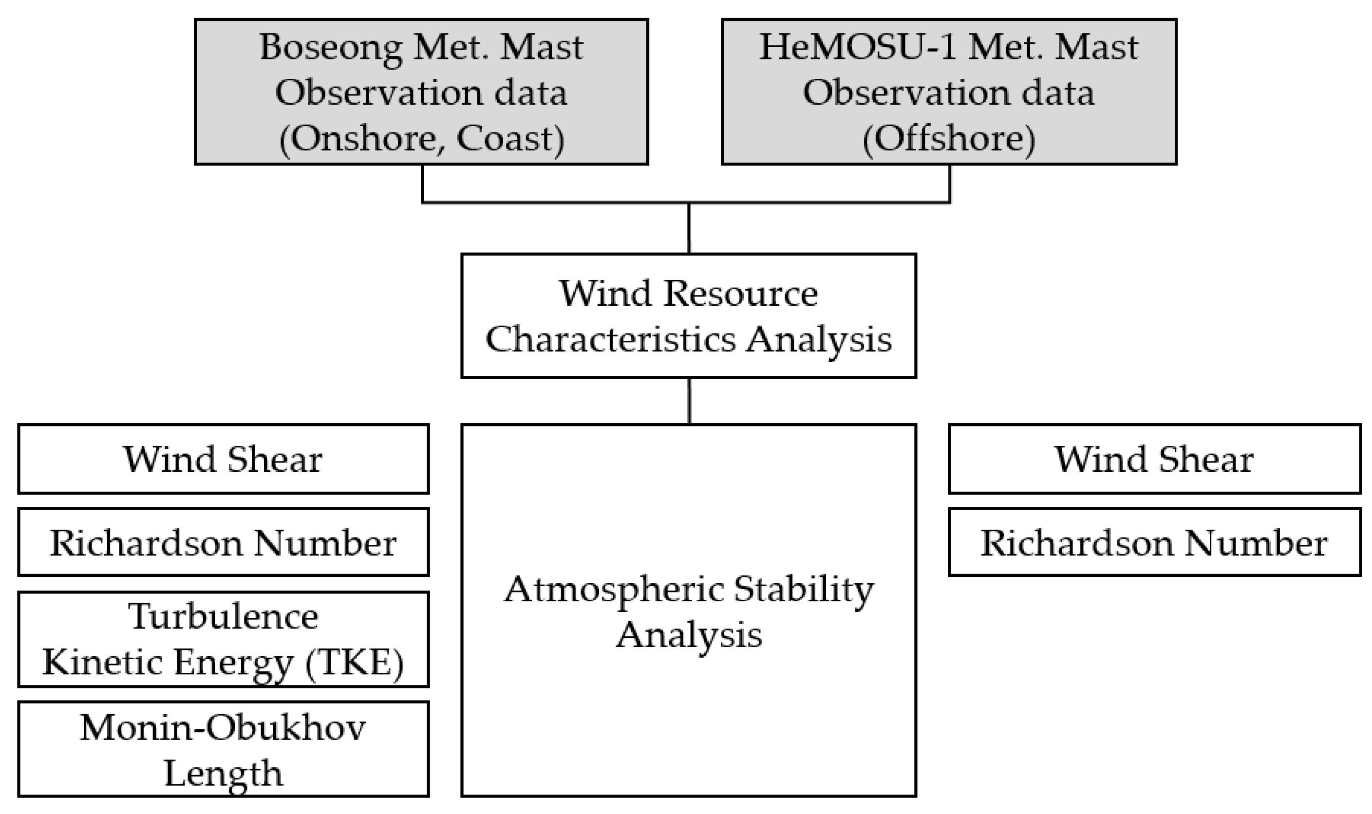
2.4. Study Procedure

The purpose of this study was to secure basic research data to analyze the characteristics of wind resources according to the atmospheric stability of the coast and the sea in order to construct an offshore wind farm. The characteristics of wind resources in each region were first analyzed through observation data from the Boseong meteorological mast built on coastal land in South Korea and the HeMOSU-1 meteorological mast installed in the West Sea.
Analysis was then performed for each atmospheric stability index, such as wind shear, Richardson number, turbulence kinetic energy, and Monin–Obukhov length (Figure 4). However, since heat flux and vertical wind speed observations are performed only at the Boseong meteorological mast, the TKE and Monin–Obukhov length were calculated only for the Boseong coast.
Prior to vitalization of the offshore wind energy industry, it is necessary to secure a lot of basic research on local meteorological characteristics that are closely related to changes in wind resources. Results of this analysis can be used as basic data for future offshore wind energy research and projects.

3. Results

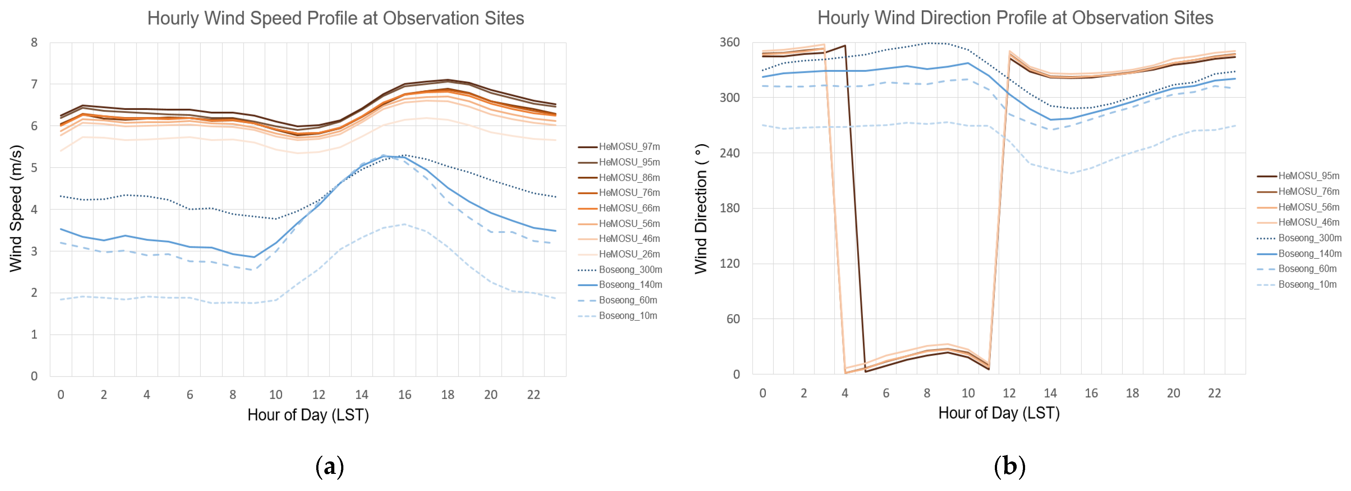
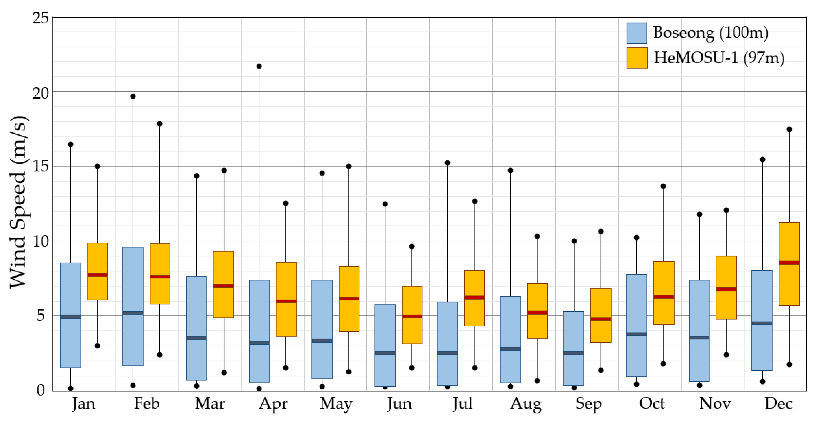
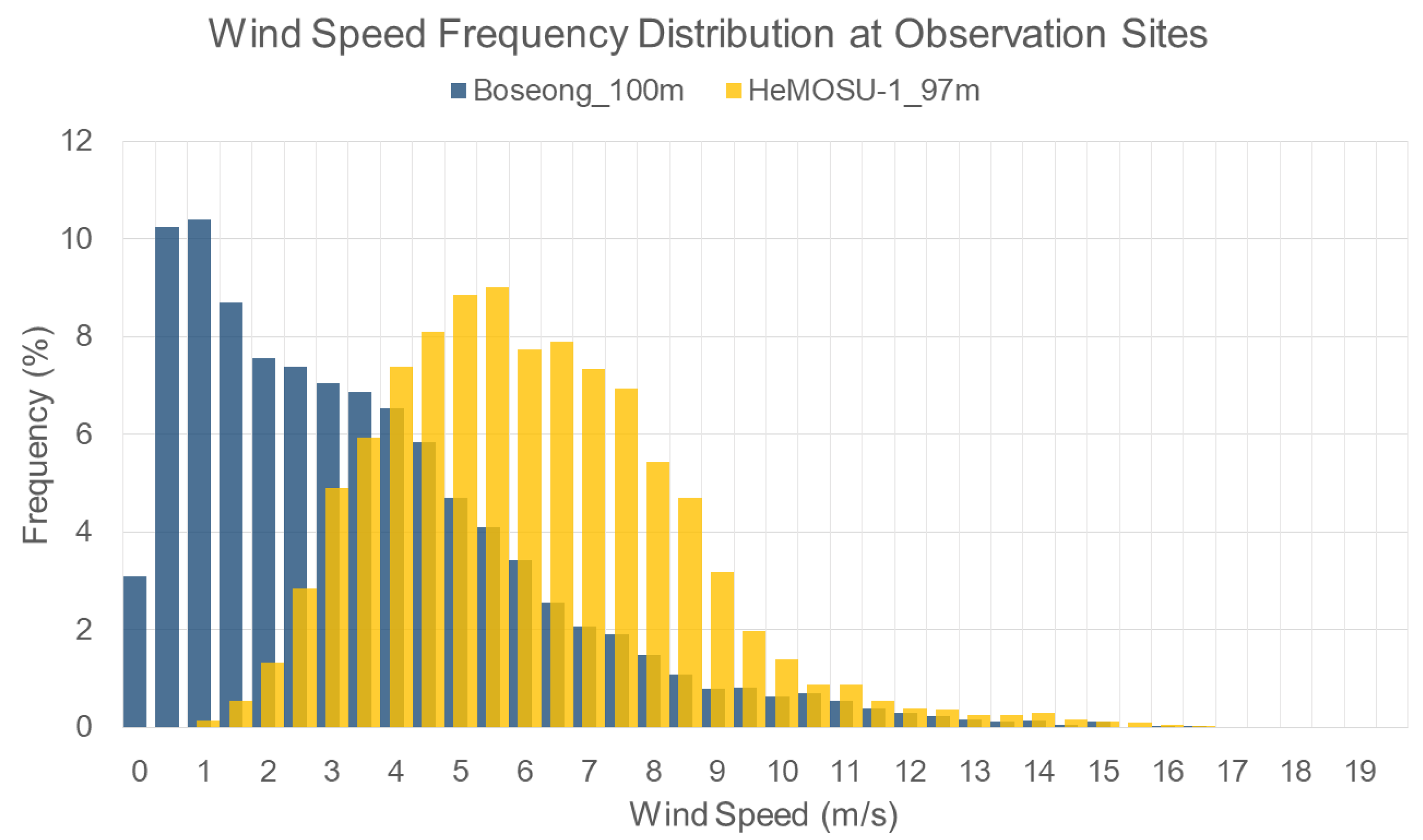
3.1. Wind Resource Characteristics

Wind speed and wind direction time series were analyzed by height based on the annual observation data of each meteorological mast (Figure 5). In the case of the coast of Boseong, it was confirmed that the wind speed by height showed the maximum value from 1500 to 1600 LST (Local Standard Time) (Figure 5a). In general, in order to increase the wind speed near the surface, an energy cascade must occur as the surface heat flux increases. A large-scale eddy then gradually becomes smaller and emits surplus energy around it.
The wind speed on the surface is strengthened by the energy released in this way. The reason that the wind speed is the strongest around 1500 LST, and not at noon, when solar radiation and heat flux are most actively transmitted, is because the surface heats up and a delay time for radiating energy is required. It is found that the 10 m wind speed is uniformly maintained at the lowest level during the day. However, upper wind speeds at 60 m, 140 m, and 300 m are similar regardless of the height as of noon, with the wind speed difference between heights decreasing. In general, as the surface heats up, the vertical convection mixing becomes active. Kinetic energy exchange between heights also becomes active. Starting at 1500 LST, wind speeds at the three heights, except near the ground, are similar at around 5 m/s. However, the wind speed difference shows a tendency to increase again around the time of sunset, when the emission of surface heat flux gradually weakens.
However, in the case of the sea, the wind speed peak occurs later than on land. This is because the specific heat of the sea is greater than that of the land, leading to enough time to retain radiation and heat flux. The wind speed peak at sea occurs between 1700 and 1800 LST. The wind speed difference between heights shows a constant pattern, with little change over time.
As the Boseong meteorological mast is located on the coast, it belongs to the sphere of influence of the sea breeze, which is a local circulation phenomenon in the coastal area. The observation area is adjacent to a bay surrounded by land in the southeast. It is greatly affected by meteorological phenomena such as winds flowing in from the corresponding direction due to the topographical characteristics of the open coast. Due to the mechanism of temperature and pressure gradients based on the difference in heat capacity between the land and ocean, sea winds from the ocean dominate during the day, while land winds dominate during the night [44]. As can be seen in Figure 5b, during the daytime, between 0900 LST and 1500 LST, the southern wind prevails and the land wind develops as it gradually changes to a northwestern wind. Overall, as local micro-meteorological phenomena in the atmospheric boundary layer around the Boseong site could be clearly identified, it could be judged that the prediction and diagnosis of meteorological phenomena would be easy.
On the other hand, the wind direction of the observation data from the offshore meteorological mast shows the characteristic of a northern wind continuously. This is because the offshore meteorological mast is far from the land, without a large-scale island area nearby. Thus, it does not fall under the sphere of influence of the land sea breeze.
Figure 6 shows the monthly averaged/maximum/minimum wind speed and deviation. The wind speed of 100 m along the coast of Boseong and the observation data of 97 m at the HeMOSU-1 meteorological mast (107 m at mean sea level when platform height is applied) are compared. In the case of the coastal wind speed in Boseong, the fluctuation range of the wind speed is larger than that of the offshore site. It is generally located in the low wind speed section of less than 5 m/s. The reason for the large fluctuation in wind speed might be due to the influence of obstacles and turbulence in the surrounding terrain. In addition, since the specific heat capacity on land is relatively small compared to that of the sea, the ratio of thermal energy to wind speed change and turbulence formation is much greater. Therefore, it seems that the fluctuation range of wind speed on land is larger than that of sea. On the other hand, in the case of the sea, the wind speed fluctuation range is small, belonging to the wind speed section of 6–7 m/s overall.
In both Boseong and the West Sea, the wind speed becomes stronger during the winter season, from around October. The wind speed decreases from around March of the following year (Figure 7).
The difference in wind resource characteristics between the coast and the sea is also clearly revealed in the results of the analysis of wind speed occurrence frequency (Figure 8). In the case of the Boseong coast, the frequency rate of the low wind speed band of 1~2 m/s is the highest, whereas the rate of the high wind speed band of 6~7 m/s is the highest in the West Sea, where the HeMOSU-1 meteorological mast is installed. When comparing with the shape parameter by Weibull distribution, the Boseong coastal site shows 1.382 and HeMOSU-1 is 2.829. The larger the shape factor, the larger the appearance ratio of a specific wind speed sector. The smaller the shape factor, the smaller the peak centered on the average wind speed and the larger the wind speed fluctuation range.

3.2. Atmospheric Stability
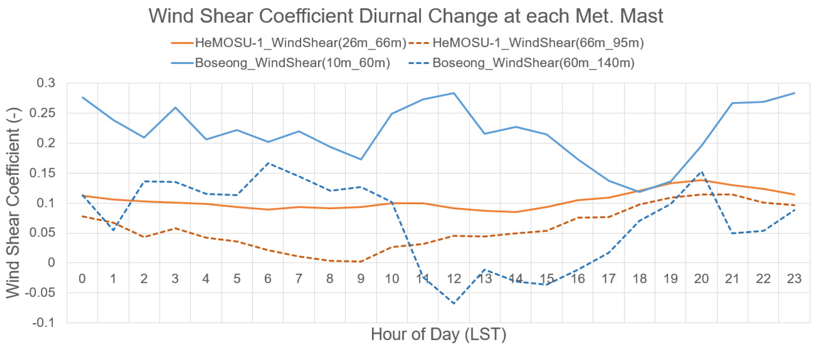
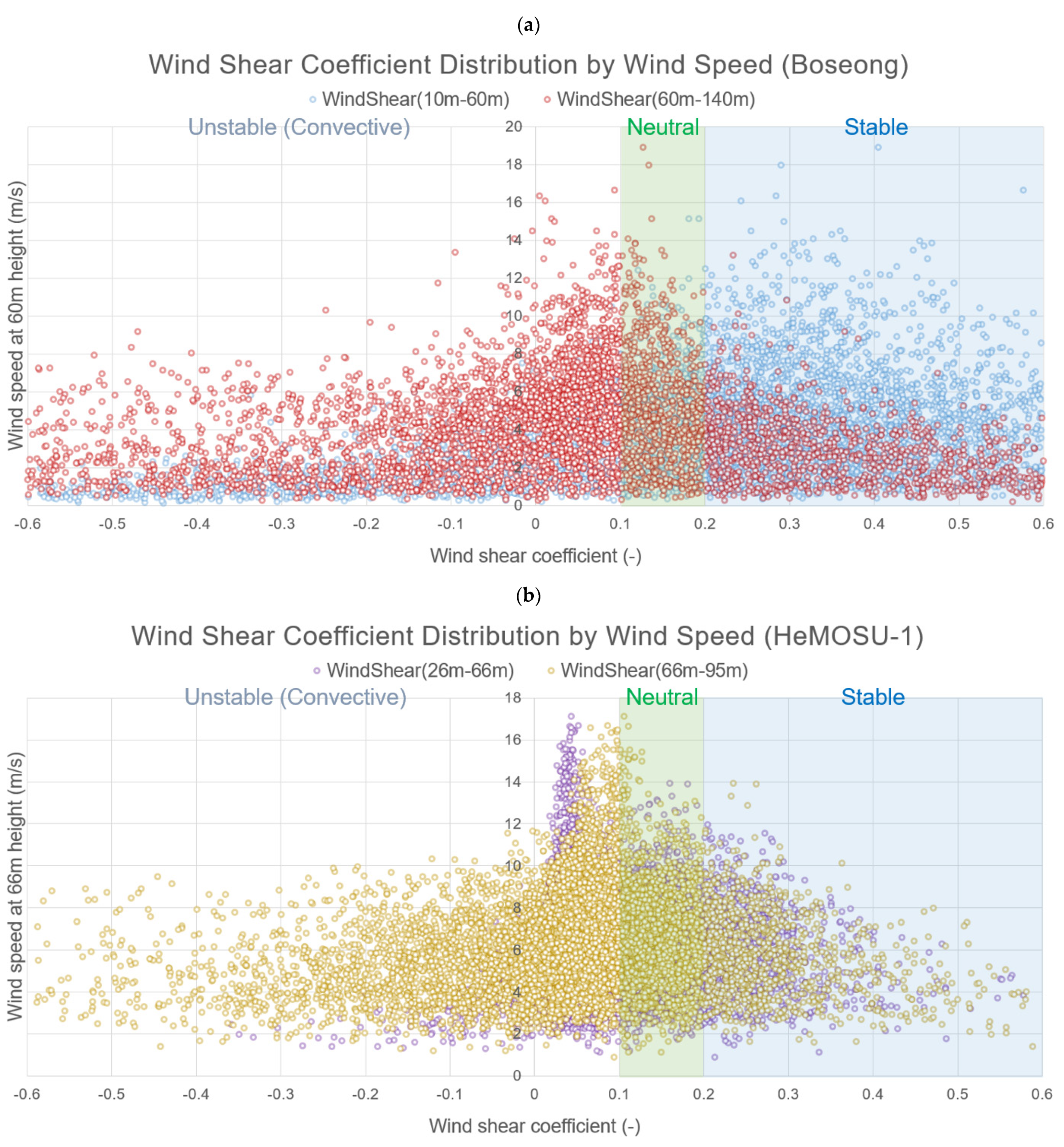
3.2.1. Wind Shear

In Figure 9, the wind shear coefficient is presented, calculated using the wind speed data for each height of the HeMOSU-1 offshore meteorological mast and the Boseong coastal meteorological mast. For the HeMOSU-1 mast, the wind shear coefficient was calculated at 26 m and 66 m height wind speeds and at 66 m and 95 m height wind speeds. For the Boseong mast, the wind shear coefficient was calculated at 10 m~60 m and 60 m~140 m height wind speeds. In the case of the Boseong site, the wind shear was calculated to determine the wind shear characteristics under the wind turbine rotor disk and near the hub height of a typical large wind turbine. However, wind shear at more than 140 m in height was excluded from the analysis because the wind speed above 140 m had a low data recovery rate due to sensor replacement.
In the case of the HeMOSU-1 offshore mast, the wind shear coefficient shows a value of 0.0~0.1 regardless of the height. This means that there is little difference in wind speed between upper and lower layers, even when the height increased. According to the classification criteria for atmospheric stability by wind shear coefficient, the atmospheric stability in the HeMOSU-1 area is unstable or near-neutral.
However, in the case of the Boseong coastal site, the difference in wind shear coefficient by height is clearly revealed. Wind shear between 10 m and 60 m appeared close to 0.3 at night, showing a high gradient wind speed difference and a mechanically stable atmospheric condition of around 0.2 on average per day. However, the wind shear between 60 m and 140 m shows a low wind shear magnitude of less than 0.15. In particular, from around noon to 1600 LST, the wind shear value is negative and the wind speed of the upper layer is weaker than that of the lower layer (Figure 10a). The ratio of mechanical atmospheric stability according to wind shear is shown in Table 5.

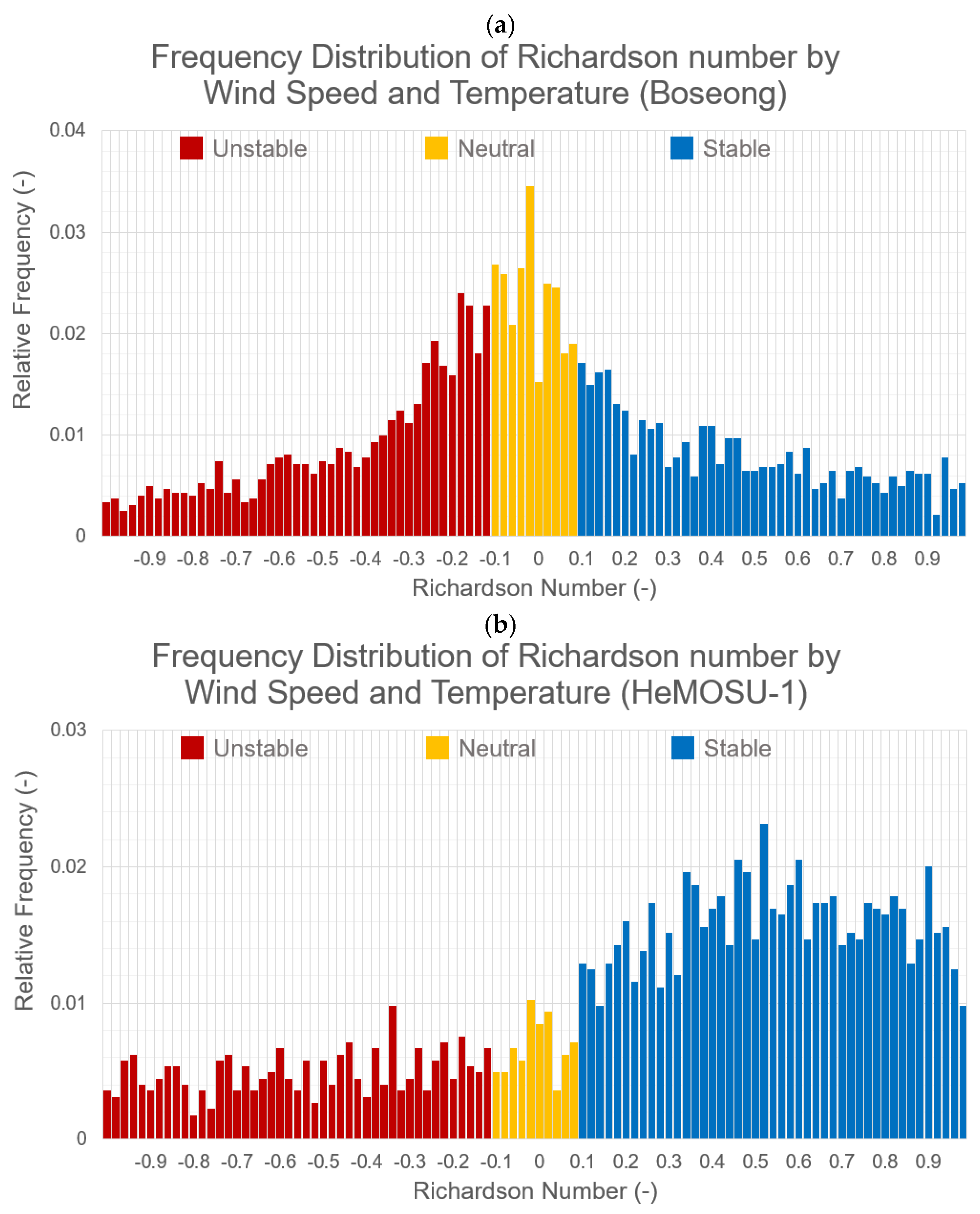
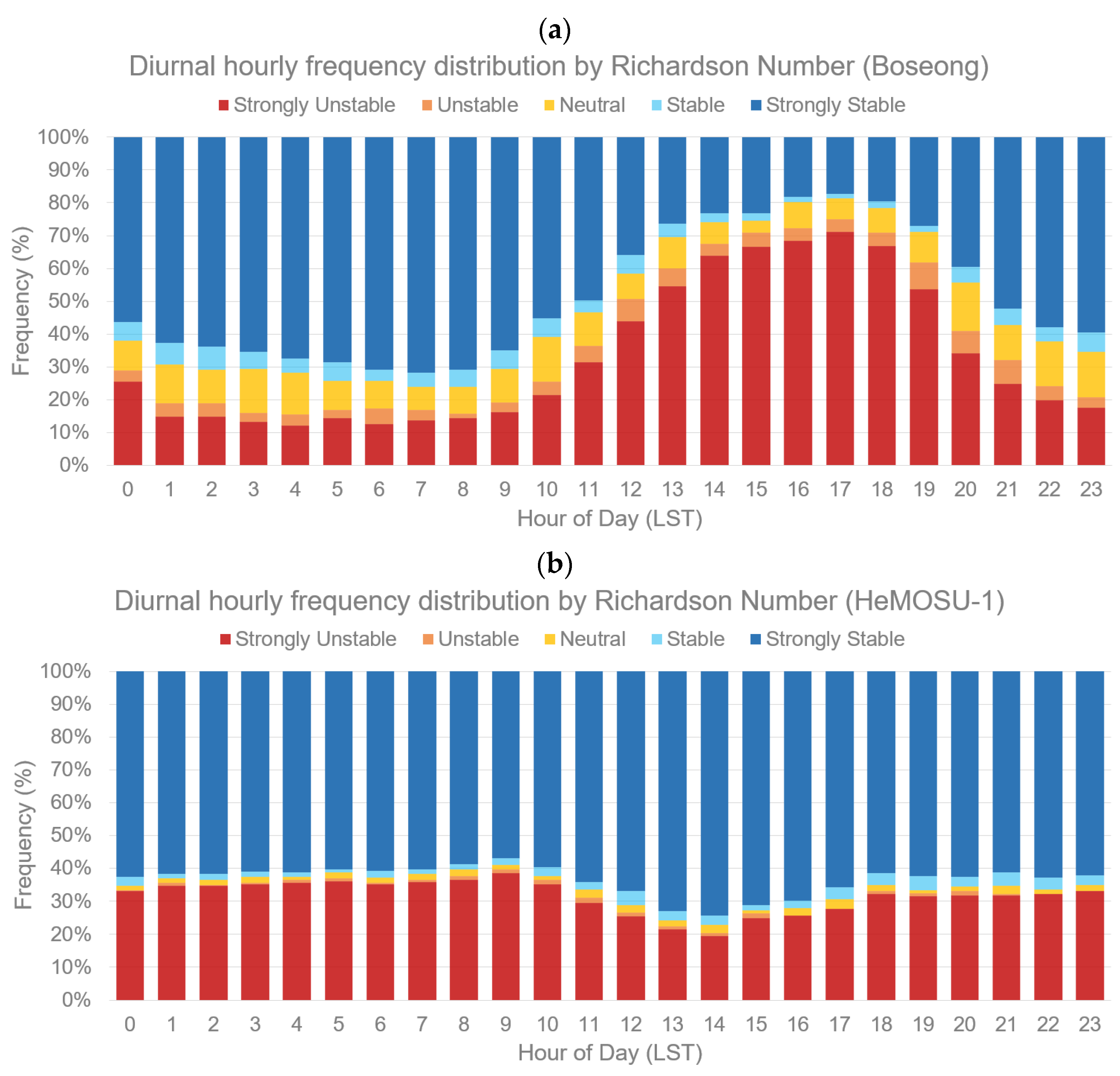
3.2.2. Richardson Number

The Richardson number is a dimensionless number calculated by applying the difference in wind speed and temperature according to height. It is used as a measure for judging dynamic atmospheric stability. In this study, air temperature data of 13 m and 94 m were used for the HeMOSU-1 offshore meteorological mast and wind speed data of 26 m and 95 m were applied to calculate the Richardson number. In the case of the Boseong coastal site, wind speeds of 10 m and 140 m and temperature data of 10 m and 140 m were used. Specific humidity and atmospheric pressure observation data are required to obtain a virtual potential temperature. Since there were no observation values, only a temperature gradient characteristic according to height was applied [25].
As a result of calculating the Richardson number based on the observation data of each meteorological mast, as can be seen in Figure 11 and Figure 12, the atmospheric stability of the Boseong coastal site showed a very ideal and typical shape. During the daytime, the ratio of unstable atmospheric condition increases due to the generation of thermal/mechanical turbulence. The atmospheric boundary layer becomes stable and stratified due to temperature inversion after sunset.
However, in the case of the offshore area, there appears to be little change in atmospheric stability by the Richardson number. Overall, a stable atmosphere accounts for more than half of the hourly rate. Most of the rest has a very unstable atmosphere. It could be seen that the atmospheric structure under the Planetary Boundary Layer (PBL) is polarized in a very stable or very unstable state (Table 6). It is judged that the change in the Richardson number is also small because differences in air temperature and wind speed by height in the offshore area are insignificant.

3.2.3. Turbulence Kinetic Energy

As could be seen from Equation (6), wind speed deviation values in the x, y, and z directions are required to calculate TKE. However, since a vertical wind speed sensor is not installed in the HeMOSU-1 offshore meteorological mast, TKE was analyzed only for the coastal area of Boseong.
TKE was calculated using observational altitude data of 10 m, 60 m, 140 m, and 300 m. The relationship between TKE and wind speed, friction velocity, or wind direction according to topographical distribution characteristics was also investigated.
If the general turbulence scale index is predicted, it can be predicted that the TKE value will be high at low heights with low wind speed bands. Figure 13 shows the frequency of occurrence (%) of TKE according to wind speed by height. The darker the red color, the more frequently TKE occurs. However, TKE shows a larger value at 300 m height than at 10 m near the surface. Wind speed variability at the upper level is also greater than that at the lower level.
The relationship between friction velocity and TKE is shown in Figure 14. The friction velocity is a key turbulence parameter representing the overturning speed of energy-containing eddies. Friction velocity can be represented by the mixing length to produce reasonable estimates of eddy viscosity in the entire boundary layer. Thus, it can be judged that when friction velocity becomes higher, the turbulence intensity also becomes higher.
It can be seen that the TKE value of the wind blowing from upper layer is high (Figure 15). As can be seen in Figure 3, where the location of the Boseong site is represented, there is a hilly area of 400~500 m to the northwest. The sea without terrain obstacles is distributed to the southeast. The low TKE value in the 120~180° wind direction zone and the high TKE value near the 300° wind direction zone by height are based on such topographical characteristics. The reason that the turbulence component of the upper wind is stronger than that near the surface is that the wind on the upwind side crosses the high hilly area.

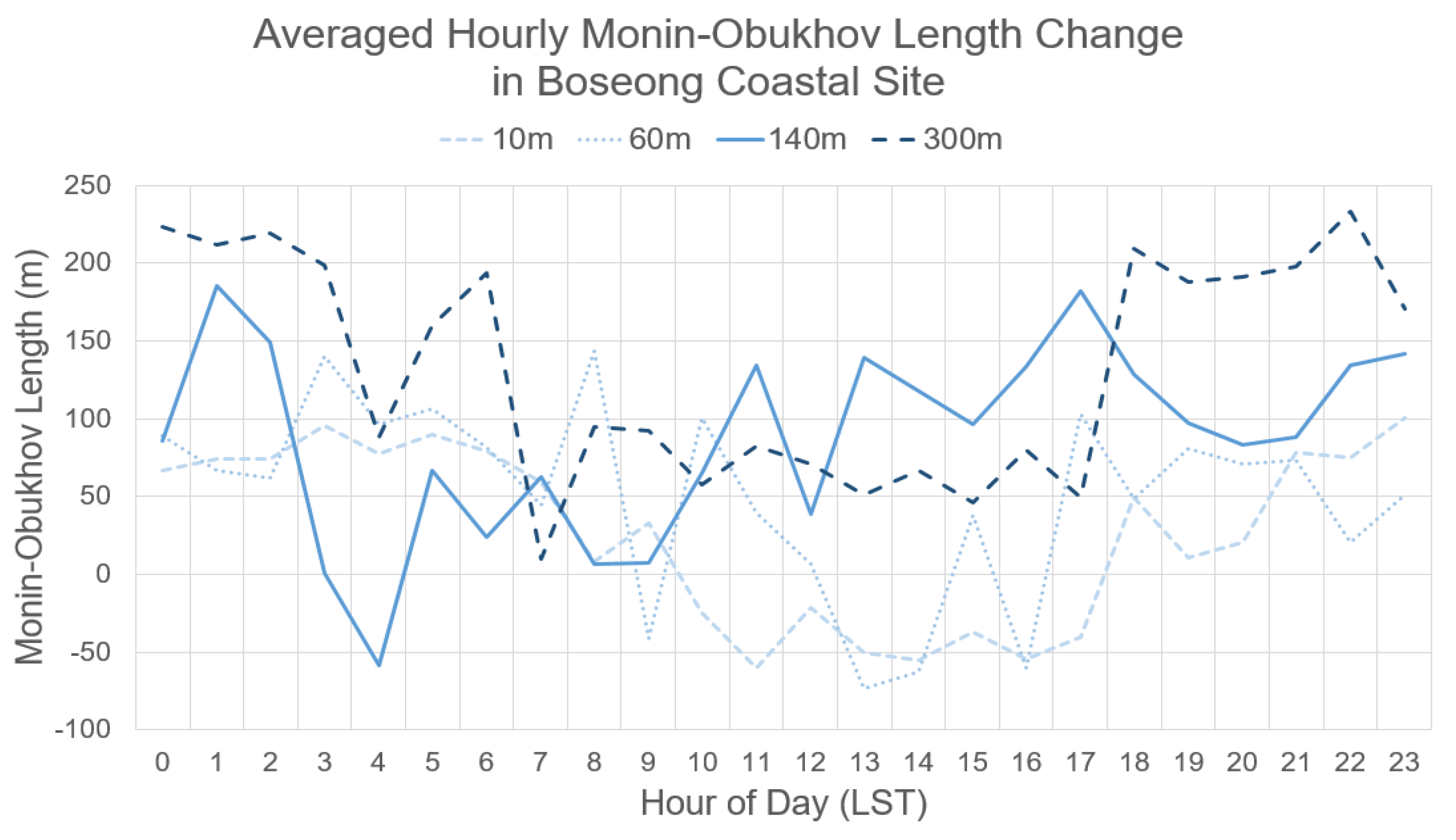
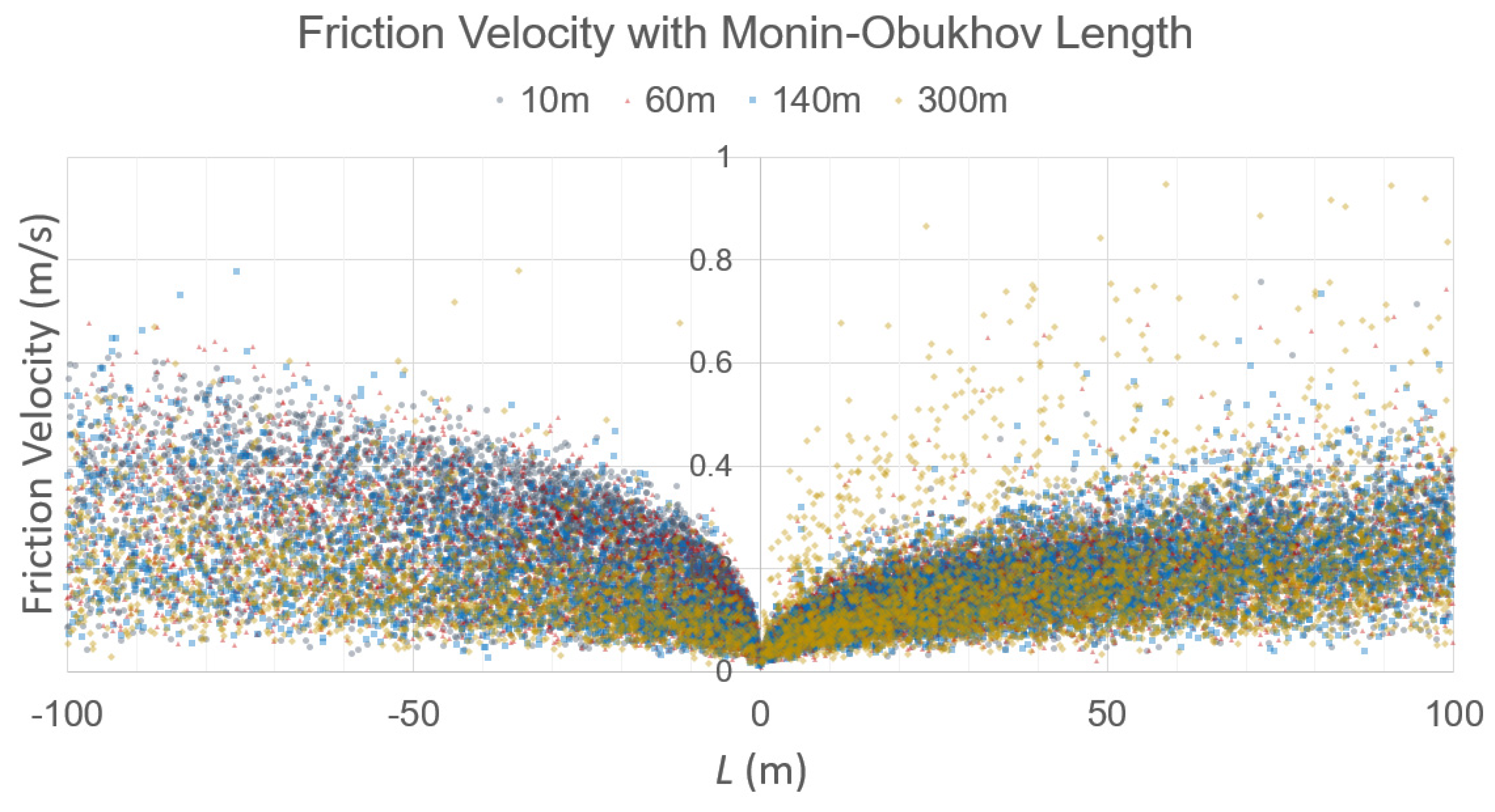
3.2.4. Monin–Obukhov Length

As with the Richardson number, the MO length is an atmospheric stability classification method that can consider both mechanical and thermal aspects. To calculate the MO length, friction velocity and heat flux measurement data are required. Since a sensor is not installed in the HeMOSU-1 offshore mast, the MO length was calculated only for the Boseong coastal site.
As can be seen in Figure 16, the diurnal change pattern is clearly reflected by the Monin–Obukhov length change at 10 m height near the surface. During the nighttime, from after sunset to before sunrise, the neutral and stable ratio increase and the atmosphere is stratified into a stable state due to surface cooling. On the other hand, during the daytime, the atmosphere becomes unstable and the movement by vertical buoyancy rather than shear dominates (Figure 16).
Table 7 shows occurrence frequency rates by atmospheric stability. In the case of the 10 m height, the frequency of the strongly unstable state is significantly higher than that of the upper layer. Its frequency decreases as the height increases. However, the frequency of occurrence of near-neutral and stable atmospheric states increases.
When comparing the daily 1-h averaged MO length change by height, values from 0900 LST to noon are negative at 10 m and 60 m heights, implying that an unstable atmosphere is dominant. However, values are positive from 1700 to 1800 LST, indicating that it is converted to a neutral or stable atmosphere (Figure 17). At 300 m height, a stable atmosphere with a continuous positive averaged value is found, similar to the results shown in Figure 18.
As a result, it is confirmed that the stability classification using the MO length is an appropriate analysis method in this study as the atmospheric stability during the day and night shows opposite patterns.

4. Conclusions

In general, the predictability of wind resources near the surface of the atmospheric boundary layer is remarkably low because it induces changes in a short time due to air convection caused by simultaneous forcing by mechanical and thermal factors, the temperature inversion layer, and wind shear caused by the vertical wind speed gradient. Since wind resource analysis based on accurate atmospheric stability is essential, the most commonly used atmospheric stability classification methods by wind shear, TKE, Richardson number, and Monin–Obukhov Length are utilized to analyze the characteristics of local wind resources according to each stability state. Wind shear and TKE are used as a classification method for mechanical stability, and the Richardson number and MO length are used for thermal stability classification.
When the atmospheric stability was analyzed by the wind shear coefficient, the diurnal change in atmospheric stability by hour was evident in the observation area of Boseong on the southern coast. During the daytime, it shows a negative coefficient value, indicating an unstable atmospheric stability state. At nighttime, the difference in wind speed between the upper and lower layers increases, indicating a positive coefficient. However, in the case of the West Sea, there is no significant change in wind shear. This might be because wind shear is mainly affected by surface roughness.
As a result of analyzing thermal atmospheric stability with the Richardson number, a clear diurnal change pattern was observed in the case of the coast of Boseong. Changes in heat flux were clearly observed in the absence of any large obstacles, which resulted in a predominantly unstable atmosphere during the daytime and a predominantly neutral and stable atmosphere at night. In the case of the West Sea, there is no significant change in heat flux over time because the specific heat of the sea is significantly higher than that of the land. Therefore, atmospheric stability also shows a lower variation pattern.
Since meteorological parameters for calculating TKE and MO lengths were observed only at the Boseong meteorological mast, it could not be analyzed in the West Sea. The TKE value of the upper wind is higher than that near the surface due to the 400 m hilly area to the northwest of the mast. A similar diurnal change pattern was found in the MO length analysis, which could have been due to thermal factors such as the Richardson number.
To further expand and improve the technological maturity of wind energy, a basic analysis of local wind resources in the area where the wind farm project will be carried out must be performed in detail. It is thought that awareness of atmospheric stability is important in order to improve the understanding of basic research in the Korean wind energy industry and to introduce professional knowledge of wind resources to operators according to obvious evidence. It is hoped that this study will be widely used as a source of basic data by developers and researchers for the detailed analysis of wind resources for offshore wind energy in South Korea.

Author Contributions

Conceptualization, G.H.R., S.J.K. and C.-J.M.; methodology, G.H.R. and M.S.C.; software, G.H.R.; validation, Y.-G.K.; formal analysis, G.H.R. and C.-J.M.; writing, G.H.R. and M.-S.J.; visualization, G.H.R. and Y.-G.K.; supervision, C.-J.M. All authors have read and agreed to the published version of the manuscript.

Funding

This work was supported by a Korea Energy Technology Evaluation and Planning (KETEP) grant funded by the Ministry of Trade, Industry and Energy (MOTIE) (No. 20203010020020).

Institutional Review Board Statement

Not applicable.

Informed Consent Statement

Not applicable.

Data Availability Statement

Not applicable.

Acknowledgments

This work was supported by a Korea Energy Technology Evaluation and Planning (KETEP) grant funded by the Ministry of Trade, Industry and Energy (MOTIE) (No. 20203010020020).

Conflicts of Interest

The authors declare no conflict of interest.

References

  1. Lee, J.-H.; Woo, J. Green New Deal Policy of South Korea: Policy Innovation for a Sustainability Transition. Sustainability 2020, 12, 10191. [Google Scholar] [CrossRef]
  2. Kim, J.-H.; Choi, K.-R.; Yoo, S.-H. Evaluating the South Korean Public Perceptions and Acceptance of Offshore Wind Farming: Evidence from a Choice Experiment Study. Appl. Econ. 2021, 53, 3889–3899. [Google Scholar] [CrossRef]
  3. Sumair, M.; Aized, T.; Gardezi, S.A.R.; Bhutta, M.M.A.; Ubaid ur Rehman, S.; Sohail Rehman, S.M. Weibull Parameters Estimation Using Combined Energy Pattern and Power Density Method for Wind Resource Assessment. Energy Explor. Exploit. 2021, 39, 1817–1834. [Google Scholar] [CrossRef]
  4. Komiyama, R.; Fujii, Y. Large-Scale Integration of Offshore Wind into the Japanese Power Grid. Sustain. Sci. 2021, 16, 429–448. [Google Scholar] [CrossRef]
  5. Samal, R.K. Assessment of Wind Energy Potential Using Reanalysis Data: A Comparison with Mast Measurements. J. Clean. Prod. 2021, 313, 127933. [Google Scholar] [CrossRef]
  6. Lee, Y.-H. Climatology of Nocturnal Low-Level Wind Maxima at a Topographically Complex Coastal Site in Boseong. Meteorol. Atmos. Phys 2021, 133, 643–653. [Google Scholar] [CrossRef]
  7. Qi, X.; Ye, Y.; Xiong, X.; Zhang, F.; Shen, Z. Research on the Adaptability of SRTM3 DEM Data in Wind Speed Simulation of Wind Farm in Complex Terrain. Arab. J. Geosci. 2021, 14, 76. [Google Scholar] [CrossRef]
  8. Plenković, I.O.; Monache, L.D.; Horvath, K.; Hrastinski, M. Deterministic Wind Speed Predictions with Analog-Based Methods over Complex Topography. J. Appl. Meteorol. Climatol. 2018, 57, 2047–2070. [Google Scholar] [CrossRef]
  9. Solbakken, K.; Birkelund, Y. Evaluation of the Weather Research and Forecasting (WRF) Model with Respect to Wind in Complex Terrain. J. Phys. Conf. Ser. 2018, 1102, 012011. [Google Scholar] [CrossRef]
  10. Jensen, D.D.; Price, T.A.; Nadeau, D.F.; Kingston, J.; Pardyjak, E.R. Coastal Wind and Turbulence Observations during the Morning and Evening Transitions over Tropical Terrain. J. Appl. Meteorol. Climatol. 2017, 56, 3167–3185. Available online: https://journals.ametsoc.org/view/journals/apme/56/12/jamc-d-17-0077.1.xml (accessed on 29 January 2022). [CrossRef]
  11. Yoo, J.-W.; Lee, H.-W.; Lee, S.-H.; Kim, D.-H. Characteristics of Vertical Variation of Wind Resources in Planetary Boundary Layer in Coastal Area using Tall Tower Observation. J. Korean Soc. Atmos. Environ. 2012, 28, 632–643. [Google Scholar] [CrossRef] [Green Version]
  12. Ryu, G.-H.; Kim, D.-H.; Lee, H.-W.; Park, S.-Y.; Kim, H.-G. A Study of Energy Production Change according to Atmospheric Stability and Equivalent Wind Speed in the Offshore Wind Farm using CFD Program. J. Environ. Sci. Int. 2016, 25, 247–257. [Google Scholar] [CrossRef]
  13. Kim, H.; Moon, C.-J.; Kim, Y.-G.; Chon, K.-H.; Joo, J.Y.; Ryu, G.H. Analysis of Atmospheric Stability for the Prevention of Coastal Disasters and the Development of Efficient Coastal Renewable Energy. J. Coast. Res. 2021, 114, 241–245. [Google Scholar] [CrossRef]
  14. Kim, D.-Y.; Kim, Y.-H.; Kim, B.-S. Changes in Wind Turbine Power Characteristics and Annual Energy Production Due to Atmospheric Stability, Turbulence Intensity, and Wind Shear. Energy 2021, 214, 119051. [Google Scholar] [CrossRef]
  15. Differences in Wind Farm Energy Production Based on the Atmospheric Stability Dissipation Rate: Case Study of a 30 MW Onshore Wind Farm-ScienceDirect. Available online: https://www.sciencedirect.com/science/article/abs/pii/S0360544221026293 (accessed on 29 January 2022).
  16. Kim, D.-Y.; Suk, K.B. Effect of Atmospheric Stability and Turbulent Kinetic Energy Dependence on Wind Turbine Power and Annual Energy Production. J. Wind Energy 2020, 11, 23–31. [Google Scholar] [CrossRef]
  17. Vanderwende, B.J.; Lundquist, J.K. The Modification of Wind Turbine Performance by Statistically Distinct Atmospheric Regimes. Environ. Res. Lett. 2012, 7, 034035. [Google Scholar] [CrossRef]
  18. Sumner, J.; Masson, C. Influence of Atmospheric Stability on Wind Turbine Power Performance Curves. J. Sol. Energy Eng. 2006, 128, 531–538. [Google Scholar] [CrossRef]
  19. St. Martin, C.M.; Lundquist, J.K.; Clifton, A.; Poulos, G.S.; Schreck, S.J. Wind Turbine Power Production and Annual Energy Production Depend on Atmospheric Stability and Turbulence. Wind Energy Sci. 2016, 1, 221–236. [Google Scholar] [CrossRef] [Green Version]
  20. Argyle, P.; Watson, S.J. Assessing the Dependence of Surface Layer Atmospheric Stability on Measurement Height at Offshore Locations. J. Wind Eng. Ind. Aerodyn. 2014, 131, 88–99. [Google Scholar] [CrossRef] [Green Version]
  21. Moon, I.-J.; Ginis, I.; Hara, T.; Thomas, B. A Physics-Based Parameterization of Air–Sea Momentum Flux at High Wind Speeds and Its Impact on Hurricane Intensity Predictions. Mon. Weather Rev. 2007, 135, 2869–2878. [Google Scholar] [CrossRef] [Green Version]
  22. Spall, M.A. Effect of Sea Surface Temperature–Wind Stress Coupling on Baroclinic Instability in the Ocean. J. Phys. Oceanogr. 2007, 37, 1092–1097. [Google Scholar] [CrossRef] [Green Version]
  23. Grylls, T.; Suter, I.; van Reeuwijk, M. Steady-State Large-Eddy Simulations of Convective and Stable Urban Boundary Layers. Bound.-Layer Meteorol. 2020, 175, 309–341. [Google Scholar] [CrossRef] [Green Version]
  24. Lebedeff, S.A.; Hameed, S. Laws of Effluent Dispersion in the Steady-State Atmospheric Surface Layer in Stable and Unstable Conditions. J. Appl. Meteorol. Climatol. 1976, 15, 326–336. [Google Scholar] [CrossRef] [Green Version]
  25. Bardal, L.M.; Onstad, A.E.; Sætran, L.R.; Lund, J.A. Evaluation of Methods for Estimating Atmospheric Stability at Two Coastal Sites. Wind Eng. 2018, 42, 561–575. [Google Scholar] [CrossRef]
  26. Wharton, S.; Lundquist, J. Atmospheric Stability Impacts on Power Curves of Tall Wind Turbines—An Analysis of a West Coast North American Wind Farm. Environ. Res. Lett. 2012, 7, 1–73. [Google Scholar] [CrossRef] [Green Version]
  27. Crosman, E.T.; Horel, J.D. Idealized Large-Eddy Simulations of Sea and Lake Breezes: Sensitivity to Lake Diameter, Heat Flux and Stability. Bound.-Layer Meteorol. 2012, 144, 309–328. [Google Scholar] [CrossRef]
  28. Barthelmie, R.J. The Effects of Atmospheric Stability on Coastal Wind Climates. Meteorol. Appl. 1999, 6, 39–47. [Google Scholar] [CrossRef]
  29. Zhan, L.; Letizia, S.; Valerio Iungo, G. LiDAR Measurements for an Onshore Wind Farm: Wake Variability for Different Incoming Wind Speeds and Atmospheric Stability Regimes. Wind Energy 2020, 23, 501–527. [Google Scholar] [CrossRef]
  30. Abkar, M.; Porté-Agel, F. Influence of Atmospheric Stability on Wind-Turbine Wakes: A Large-Eddy Simulation Study. Phys. Fluids 2015, 27, 035104. [Google Scholar] [CrossRef] [Green Version]
  31. Wharton, S.; Lundquist, J.K. Atmospheric Stability Affects Wind Turbine Power Collection. Environ. Res. Lett. 2012, 7, 014005. [Google Scholar] [CrossRef]
  32. Wharton, S.; Lundquist, J.K. Assessing Atmospheric Stability and Its Impacts on Rotor-disk Wind Characteristics at an Onshore Wind Farm. Wind Energy 2012, 15, 525–546. [Google Scholar] [CrossRef]
  33. Sucevic, N.; Djurisic, Z. Influence of atmospheric stability variation on uncertainties of wind farm production estimation. In Proceedings of the European Wind Energy Conference & Exhibition, Copenhagen, Denmark, 16–19 April 2012. [Google Scholar]
  34. Hwang, S.E.; Lee, Y.T.; Shin, S.S.; Kim, K.H. Study on the Local Weather Characteristics using Observation Data at the Boseong Tall Tower. J. Korean Earth Sci. Soc. 2020, 41, 459–468. [Google Scholar] [CrossRef]
  35. Lim, H.-J.; Lee, Y.-H. Characteristics of Sea Breezes at Coastal Area in Boseong. Atmosphere 2019, 29, 41–51. [Google Scholar] [CrossRef]
  36. Ko, D.-H.; Cho, H.-Y.; Lee, U.-J. Estimation and Analysis of the Vertical Profile Parameters using HeMOSU-1 Wind Data. J. Korean Soc. Coast. Ocean Eng. 2021, 33, 122–130. [Google Scholar] [CrossRef]
  37. Kim, D.-Y.; Jeong, H.-S.; Kim, Y.-H.; Kim, B.-J. Comparative Assessment of Wind Resources Between West Offshore and Onshore Regions in Korea. Atmosphere 2018, 28, 1–13. [Google Scholar] [CrossRef]
  38. Chen, G.; Rong, L.; Zhang, G. Numerical Simulations on Atmospheric Stability Conditions and Urban Airflow at Five Climate Zones in China. Energy Built Environ. 2021, 2, 188–203. [Google Scholar] [CrossRef]
  39. Gualtieri, G. Atmospheric Stability Varying Wind Shear Coefficients to Improve Wind Resource Extrapolation: A Temporal Analysis. Renew. Energy 2016, 87, 376–390. [Google Scholar] [CrossRef]
  40. Ray, M.L.; Rogers, A.L.; Mcgowan, J.G. Analysis of Wind Shear Models and Trends in Different Terrains. 2006, pp. 1–14. Available online: https://citeseerx.ist.psu.edu/viewdoc/download?doi=10.1.1.574.7468&rep=rep1&type=pdf (accessed on 29 December 2021).
  41. Nappo, C.J. (Ed.) 6—Waves and Turbulence. In An Introduction to Atmospheric Gravity Waves; International Geophysics Series; Academic Press: Cambridge, MA, USA, 2002; Volume 85, pp. 125–154. [Google Scholar]
  42. Stival, L.; Oliveira de Andrade, F.; Guetter, A. The Impact of Wind Shear and Turbulence Intensity on Wind Turbine Power Performance. Espaço Energ. 2007, 27, 11–20. [Google Scholar]
  43. Ryu, G.-H.; Kim, D.-H.; Lee, H.-W.; Park, S.-Y.; Yoo, J.-W.; Kim, H.-G. Accounting for the Atmospheric Stability in Wind Resource Variations and Its Impacts on the Power Generation by Concentric Equivalent Wind Speed. J. Korean Sol. Energy Soc. 2016, 36, 49–61. [Google Scholar] [CrossRef]
  44. Reddy, T.V.R.; Mehta, S.K.; Ananthavel, A.; Ali, S.; Annamalai, V.; Rao, D.N. Seasonal Characteristics of Sea Breeze and Thermal Internal Boundary Layer over Indian East Coast Region. Meteorol. Atmos. Phys. 2021, 133, 217–232. [Google Scholar] [CrossRef]
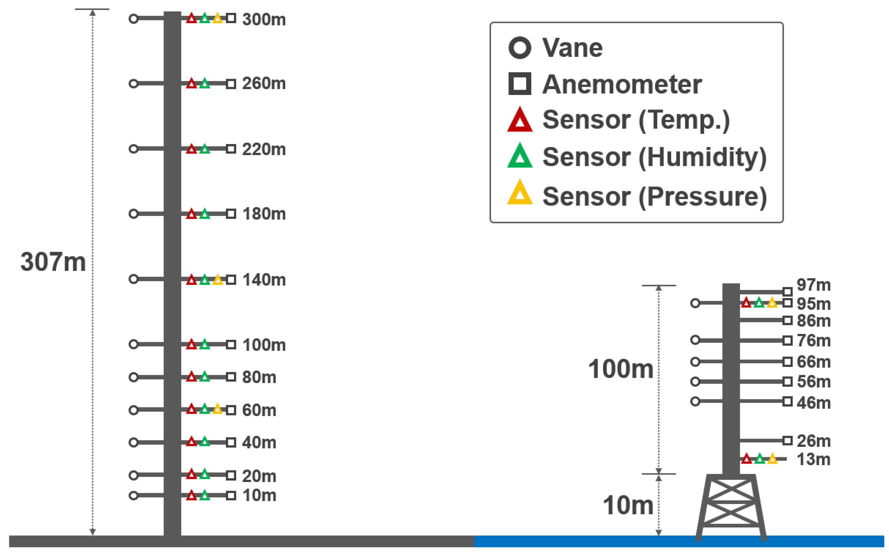
Figure 1. Site photography of both meteorological masts. Top: HeMOSU-1 offshore mast; Bottom: Boseong onshore mast.
Energies 15 01305 g001
Figure 2. Sensor installation heights for each meteorological mast. Left: Boseong onshore mast; Right: HeMOSU-1 offshore mast.
Energies 15 01305 g002
Figure 3. Satellite view and site photography of the installation of Boseong Global Standard Meteorological Observatory site.
Energies 15 01305 g003
Figure 4. Study procedure overview.
Energies 15 01305 g004
Figure 5. Hourly change in wind speed and direction: (a) 1-hourly averaged diurnal wind speed change; (b) 1-hourly averaged wind direction change. Blue color indicates Boseong coastal meteorological mast; orange color indicates HeMOSU-1 offshore meteorological mast.
Energies 15 01305 g005
Figure 6. Box plots of observed wind speed data. The top of the box indicates the daily-averaged high. The bottom indicates the daily-averaged low. Top and bottom of the line indicate the maximum and minimum values of 10-min averaged data, respectively.
Energies 15 01305 g006
Figure 7. Data maps of observed wind speed data. (a) Boseong mast (10 m); (b) Boseong mast (140 m); (c) HeMOSU-1 mast (26 m); (d) HeMOSU-1 mast (95 m).
Energies 15 01305 g007
Figure 8. Wind speed frequency distribution at each observation site. Dark blue-colored bars represent Boseong meteorological mast data. Yellow-colored bars represent HeMOSU-1 data.
Energies 15 01305 g008
Figure 9. Wind shear coefficient diurnal change at each observation site. Blue-colored lines represent Boseong meteorological mast data. Orange-colored lines represent HeMOSU-1 data.
Energies 15 01305 g009
Figure 10. Wind speed is correlated with wind shear coefficient. (a) Boseong mast (blue-colored circles represent wind shear between 10 m and 60 m; red-colored circles represent wind shear between 60 m and 140 m). (b) HeMOSU-1 mast (purple-colored circles represent wind shear between 26 m and 66 m; yellow-colored circles represent wind shear between 66 m and 95 m).
Energies 15 01305 g010
Figure 11. Frequency distribution is correlated with Richardson number. Each colored bar represents unstable (red), neutral (yellow), and stable (blue) conditions; (a) Boseong; (b) HeMOSU-1.
Energies 15 01305 g011
Figure 12. Diurnal hourly frequency distribution is correlated with Richardson number. Each colored bar represents strongly unstable (red), unstable (orange), neutral (yellow), stable (sky blue), and strongly stable (dark blue) conditions; (a) Boseong; (b) HeMOSU-1.
Energies 15 01305 g012
Figure 13. Data maps of observed occurrence frequency (%) of wind speed data as function of TKE. (a) Boseong mast (10 m); (b) Boseong mast (140 m); (c) HeMOSU-1 mast (26 m); (d) HeMOSU-1 mast (95 m).
Energies 15 01305 g013
Figure 14. Correlation between TKE and friction velocity at Boseong meteorological mast. (a) 10 m, (b) 60 m, (c) 140 m, and (d) 300 m heights.
Energies 15 01305 g014
Figure 15. TKE calculated for the whole analyzed period as a function of wind direction at Boseong meteorological mast. (a) 10 m, (b) 60 m, (c) 140 m, and (d) 300 m heights.
Energies 15 01305 g015
Figure 16. Scatter plot analysis for diurnal change in atmospheric stability at 10 m height by Monin–Obukhov length. Red dots represent 10-min averaged MO length data at each hour. Dark solid line represents hourly averaged MO length.
Energies 15 01305 g016
Figure 17. Diurnal change in 1 h averaged Monin–Obukhov length at each height. Each colored line represents 10 m height (short dashed light blue line), 60 m height (dotted light blue line), 140 m height (solid blue line), and 300 m height (long dashed dark blue line).
Energies 15 01305 g017
Figure 18. Scatter plot for the correlation between friction velocity and Monin–Obukhov length. Each colored symbol represents combined data at 10 m height (gray circle), 60 m height (red triangle), 140 m height (blue square), and 300 m height (yellow diamond).
Energies 15 01305 g018
Table 1. Observation parameters and heights for each meteorological mast.
ItemObservation Height [m]
Boseong Met. Mast (Onshore, Coast)Wind speed10, 20, 40, 60, 80, 100, 140, 180, 220, 260, 300
Wind direction10, 20, 40, 60, 80, 100, 140, 180, 220, 260, 300
Air temperature10, 20, 40, 60, 80, 100, 140, 180, 220, 260, 300
Air pressure60, 140, 300
Relative humidity10, 20, 40, 60, 80, 100, 140, 180, 220, 260, 300
HeMOSU-1 Met. Mast (Offshore)Wind speed 126, 46, 56, 66, 76, 86, 95, 97
Wind direction 146, 56, 66, 76, 95
Air temperature 113, 95
Air pressure 113, 95
Relative humidity 113, 95
1 To correctly calculate the measuring height above the mean sea level (MSL), the height of the sensor above MSL (≃10.0 m) must be considered. For example, if the configured measuring height of HeMOSU-1 is 10.0 m, true height where measurement is taken is 20.0 m above the Lowest Astronomical Tide (LAT).
Table 2. Specifications of Boseong global standard meteorological observation site and its meteorological observation elements.
ItemDescription
NameBoseong Global Standard Meteorological Observation Site
Location34.76° N, 127.21° E
Height [m]307.19
Level [m]10, 20, 40, 60, 80, 100, 140, 180, 220, 260, 300 (11 levels)
Observation factorsWind speed, wind direction, air temperature, radiation, relative humidity, air pressure, CO2·H2O concentration
Calculation or external factorsMomentum flux, sensible heat flux, air density, latent heat flux, roughness length, friction velocity
Period1 January 2016~31 December 2016 (10 min)
Table 3. Specification of HeMOSU-1 offshore meteorological mast and its observation elements.
ItemDescription
NameHeMOSU-1 (HErald Meteorological and Oceanographic Special Unit-1)
Location35.47° N, 126.13° E
Height [m]100.0
Level [m]26, 46, 56, 66, 76, 86, 95, 97 (8 levels)
Observation factorsWind speed, wind direction, air temperature, relative humidity, air pressure
Period1 January 2016~31 December 2016 (10 min)
Table 4. Atmospheric stability indices criteria and boundary layer properties.
Stability ClassWind ShearRichardson NumberTKE 1
[m2/s2]
MO 2 Length
[m]
Boundary Layer Properties
Strongly Unstable α < 0.0Ri < −0.86TKE > 1.4−50 m < L ≤ 0 mLowest WS 3/Shear
Highly TI
Unstable 0.0     α < 0.1−0.86 ≤ Ri < −0.11.0 < TKE < 1.4−600 m < L ≤ −50 mLower WS/Shear
High TI
Near-Neutral 0.1     α < 0.2−0.1 ≤ Ri < 0.0530.7 < TKE < 1.0 | L | > 600 mLogarithmic
wind profile
Stable 0.2     α < 0.30.053 ≤ Ri < 0.1340.4 < TKE < 0.7100 m < L ≤ 600 mHigh WS/Shear
Low TI
Strongly Stable α ≥ 0.3Ri ≥ 0.134TKE < 0.40 m < L ≤ 100 mHighest WS/Shear
Lowest TI
1 Turbulence kinetic energy, 2 Monin–Obukhov, 3 wind speed.
Table 5. Atmospheric stability ratio by wind shear coefficient.
Met. MastHeight [m]Atmospheric Stability Criteria by Wind ShearAll
Strongly
Unstable
(α < 0)
Unstable
(0 ≤ α < 0.1)
Neutral
(0.1 ≤ α < 0.2)
Stable
(0.2 ≤ α < 0.3)
Strongly
Stable
(α ≥ 0.3)
Boseong
(Coast)
10–6022.19%9.18%14.61%15.52%38.50%100%
60–14038.25%18.56%12.69%7.95%22.55%100%
HeMOSU-1
(Offshore)
26–664.44%59.07%24.38%10.04%2.07%100%
66–9526.47%41.71%20.44%7.79%3.59%100%
Table 6. Atmospheric stability ratio by Richardson number.
Met.
Mast
Height
[m]
Atmospheric Stability Criteria by Richardson NumberAll
Strongly
Unstable
(Ri < −0.86)
Unstable
(−0.86 ≤ Ri < −0.1)
Neutral
(−0.1 ≤ Ri < 0.053)
Stable
(0.053 ≤ Ri < 0.134)
Strongly
Stable
(Ri ≥ 0.134)
Boseong
(Coast)
10–14032.98%4.30%9.83%4.31%48.58%100%
HeMOSU
(Offshore)
26–9531.55%0.75%1.74%2.52%63.44%100%
Table 7. Atmospheric stability ratio by Monin–Obukhov length.
Met.
Mast
Heigh
[m]
Atmospheric Stability Criteria by Monin–Obukhov LengthAll
Strongly
Unstable
(−50 ≤ L < 0)
Unstable
(−600 ≤ L < −50)
Neutral
(|L| > 600)
Stable
(100 < L ≤ 600)
Strongly
Stable
(0 < L ≤ 100)
Boseong
(Coast)
1020.3820.033.3614.7241.51100%
6010.4123.316.8617.7341.69100%
1407.2722.789.1021.2639.29100%
3007.3426.0814.0227.3925.17100%
Publisher’s Note: MDPI stays neutral with regard to jurisdictional claims in published maps and institutional affiliations.

