
Research on Fuel Cell Fault Diagnosis Based on Genetic Algorithm Optimization of Support Vector Machine †


1
School of Mechanical and Electrical Engineering, Beijing Information Science & Technology University, Beijing 100092, China
2
Collaborative Innovation Center of Electric Vehicles in Beijing, Beijing Information Science & Technology University, Beijing 100092, China
3
Key Laboratory of Modern Measurement and Control Technology, Ministry of Education, Beijing Information Science & Technology University, Beijing 100192, China
4
National Engineering Laboratory for Electric Vehicles, Beijing Institute of Technology, Beijing 100081, China
5
Guangzhou Automobile Group Co., Ltd., Automotive Engineering Research Institute, Guangzhou 510006, China
*
Author to whom correspondence should be addressed.
†
This paper is an extended version of our paper presented at the International Conference on Electric and Intelligent Vehicles (ICEIV2021), Nanjing, China, 25–28 June 2021; Paper number: 12601219.
Energies 2022, 15(6), 2294; https://doi.org/10.3390/en15062294
Submission received: 5 October 2021
/
Revised: 24 December 2021
/
Accepted: 27 December 2021
/
Published: 21 March 2022
(This article belongs to the Special Issue Selected Papers from the International Conference on Electric and Intelligent Vehicles (ICEIV 2021) on Advanced Energy Storage System)
Abstract
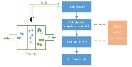
:The fuel cell engine mechanism model is used to research fault diagnosis based on a data-driven method to identify the failure of proton exchange membrane fuel cells in the process of operation, which leads to the degradation of system performance and other problems. In this paper, an extreme learning machine and a support vector machine are applied to classify the usual faults of fuel cells, including air compressor faults, air supply pipe and return pipe leaks, stack flooding faults and temperature controller faults. The accuracy of fault classification was 78.67% and 83.33% respectively. In order to improve the efficiency of fault classification, a genetic algorithm is used to optimize the parameters of the support vector machine. The simulation results show that the accuracy of fault classification was improved to 94% after optimization.
1. Introduction
A proton exchange membrane fuel cell (PEMFC) can be regarded as a power generation system, which produces water after a chemical reaction occurs between hydrogen and oxygen. The characteristics of PEMFCs are high energy conversion efficiency, high efficiency, no pollution, low noise and easy maintenance. They have broad application prospects in electric vehicles, trams, and other transportation fields [1]. The operation of PEMFCs involves the coupling of thermal, electric and flow features. The internal structure of a PEMFC is complicated. Since the output is easily affected by the external environment, various faults are prone to occur inside the fuel cell during operation. The output performance of the system is reduced, which eventually leads to system failure. When there is an open fire, reactor overload or hydrogen leakage can cause serious combustion or explosive damage. However, efficient fault diagnosis can grasp the fault status of the fuel cell in time, and always maintain good working performance [2]. It is helpful to improve the performance and service life of PEMFCs by using accurate and fast fault diagnosis and control measures.
Common faults in fuel cell systems include the internal failure of the air compressor, the leakage failure of the gas supply or return manifold, the internal flooding or dry failure of the stack, as well as the failure of the water and heat management system during the working process [3]. The air compressor is a crucial part of the fuel cell cathode air supply system for vehicles. The performance of the air compressor directly affects the efficiency, compactness and water balance of the fuel cell system. The gas supply system includes a hydrogen supply system and an oxygen supply system. There is a danger of explosion if the hydrogen supply manifold leaks. Flooding failure of the stack will reduce the output performance of the fuel cell and reduce its durability. A serious drying failure will cause the proton exchange membrane to rupture, which cause irreparable losses. The failure of the hot water management system will also seriously affect the operation of the fuel cell. At present, there have been many studies on the diagnosis of fuel cell faults.
Won et al. [4] adopted a strategy of combining modelling and data. Aiming at the six types of faults in air supply pipelines, artificial neural networks were used as fault classifiers. The method based on residual error can solve the limitations of fault diagnosis. Liu et al. [5] proposed a method to solve the leakage of a gas supply system. The over-oxygen rate obtained from the model and the observer was compared in order to estimate the fault state and the fault signal. Zuo et al. [6] proposed a diagnosis method for flooding faults under variable load conditions. The authors proposed to use the convolutional neural network to establish the fault diagnosis model and used the normalization method to enhance the generalization ability of the model. Zhou et al. [7] proposed a method based on wavelet changes for rotating surge failure in the air compressor under low flow conditions. This method can issue an alarm within 1 s when a fault occurs. Lim et al. [8] proposed a fault diagnosis strategy using a residual basis scaling method by analyzing the experimental data under different current densities for the five faults of the fuel cell thermal management system. Zhuo et al. [9] proposed a fault diagnosis method for DCDC converters. By selecting the inductor current of the main controller for detection, the use of sensors was reduced. This method is robust. Shao et al. [10] proposed a method based on an artificial neural network. The model of neural network integration was built by analyzing the artificial neural network integration method. The fuel cell fault analysis was carried out by using the model to improve the wide range of application. Li et al. [11] proposed to use effective informed adaptive particle swarm optimization (EIA-PSO) to predict the output voltage and the power of a fuel cell. Liu et al. [12] combined the extreme learning machine (ELM) algorithm with the Dempster-Shafer (DS) algorithm for fault diagnosis. The ELM algorithm was used for the preliminary judgment of faults. The DS algorithm was used to output the diagnosis result. The fault resolution accuracy of this method can reach more than 98%. Wu and Ye [13] proposed a fault diagnosis strategy using an LS-SVM classifier. In the article, the HSMMs technology was used to estimate the life of the fuel cell. Zhao et al. [14] proposed their own methods for identifying single-sensor faults and serious system faults. They first studied on the interaction between different sensors, and used PCA to extract the fault characteristics. Djeziri et al. [15] set up a health indices (HIs) model for the safety of fuel cells. When the predicted value and the measured value of the established HI model exceed the threshold, the model was updated to monitor the working status of the fuel cell in real time. Du et al. [16] used the parameters obtained from the three types of faults at different levels to train the fault classification model, which reduced the probability of misjudgement. Zhang and Guo [17] proposed a fuel cell fault diagnosis method related to a convolutional neural network. They extracted high-dimensional features from the original data set and transformed them into feature maps. The graph was imported into the convolutional neural network to realize the classification of faults.
Although many researchers have accomplished a good deal of research and exploration on PEMFC fault diagnosis [18,19], the research still lags behind other technologies in fuel cell. Some technical challenges still exist. The methods that have been proposed so far mainly focus on the ability to detect some specific faults. Research on fault isolation and analysis has been neglected. Based on a 75 kW fuel cell engine simulator model, this paper proposes the diagnosis parameters of the common faults with the PEMFC as the original fault. Many researchers have used this model in their research. The two classification methods of ELM and SVM are used to train fault diagnosis models for fault diagnosis. The genetic algorithm is used to improve the parameters of the kernel function and penalty factor of the SVM algorithm. Finally, the fault classification results of the three algorithms are analyzed, which proves that the optimized algorithm is beneficial to enhance the efficiency of fault diagnosis. This article helps operators of fuel cell vehicles to diagnose and deal with faults during operation to improve driving safety in relation to fuel cell vehicles.
2. Fault Classification Method
2.1. Extreme Learning Machine Theory
ELM is a new type of fast-learning algorithm based on a feedforward neural network [20], which has the characteristics of fast training speed, little reliance on labeled samples and high accuracy. ELM is used in many fields. The network structure of an ELM is shown in Figure 1.
In Figure 1, is the network input, is the network output, is the number of neurons in the hidden-layer. is the input weight from the input layer to the hidden layer, which is expressed as:
is the threshold value of hidden-layer neurons, which is expressed as follows:
is the output weight from hidden layer to the output layer. In a limit-learning machine, is determined by us. Thus, the network parameters are input weight , hidden layer neuron threshold and output weight .
In practice, the extreme learning machine includes two processes: training and prediction.
In the training process, after knowing the input and output of the extreme learning machine training sample, the transformation method between the input and output is easy to obtain. An extreme learning machine with the training samples and neurons in the hidden layer can be expressed as:
In Equation (3), is the input weight, is the threshold value of the neuron in the hidden layer, is the output weight, is the inner product of and , and is the activation function.
When the error between the network output and the sample output is minimal, as shown in Equation (4),
Expressed as a matrix:
where is the output of the hidden layer neuron, is the output weight and is sample output.
In ELM, if the input weight and threshold are given randomly or artificially, then the matrix in Equation (5) is well-determined. The output weight can be calculated as the following Equation (9):
In the prediction process, the mapping relation of the input and output of the extreme learning machine is known, and the output of ELM is calculated.
In the process of prediction, the input weight , threshold value and output weight of ELM are known. Given sample input , sample output can be obtained according to Equations (5)–(8).
2.2. Support Vector Machine Theory
The classification principle of SVM is to map fault feature vectors in the original space to the kernel space using the kernel method, and converting the fault data that are not separable in the original space into linearly separable or approximately linearly separable data in the kernel space [21]. The basic theory of SVM only supports the binary classification problem, which uses a classification hyperplane to separate the data for two different characteristics.
Taking category 1 and category 2 as training samples, are marked as . The general form of the linear discriminant function of the input space is:
where is a constant on a high-dimensional plane and is a constant. After the normalization process, all samples met:
Therefore, the classification interval is obtained. When takes the minimum value, the interval is the maximum. The problem is transformed into the following secondary planning stage:
Using the Lagrange method, the corresponding Lagrange function can be obtained as follows:
Among these, the Lagrange coefficient is recognized as . By setting the derivative of and to zero, the following conditions can be obtained:
Incorporating Equations (14) and (15) into Equation (13), the dual problem of the original objective function is obtained.
Solving the optimal solution of , the optimal hyperplane can be calculated as
where .
The process of training and decision-making is only related to the inner product between the training samples. Thus, the kernel function can be directly introduced to complete the extension from linear problems to nonlinear problems. When using SVM to solve practical problems, the choice of kernel function is critical. It is often necessary to construct corresponding kernel functions according to specific problems.
3. Fault Simulation of Fuel Cell System
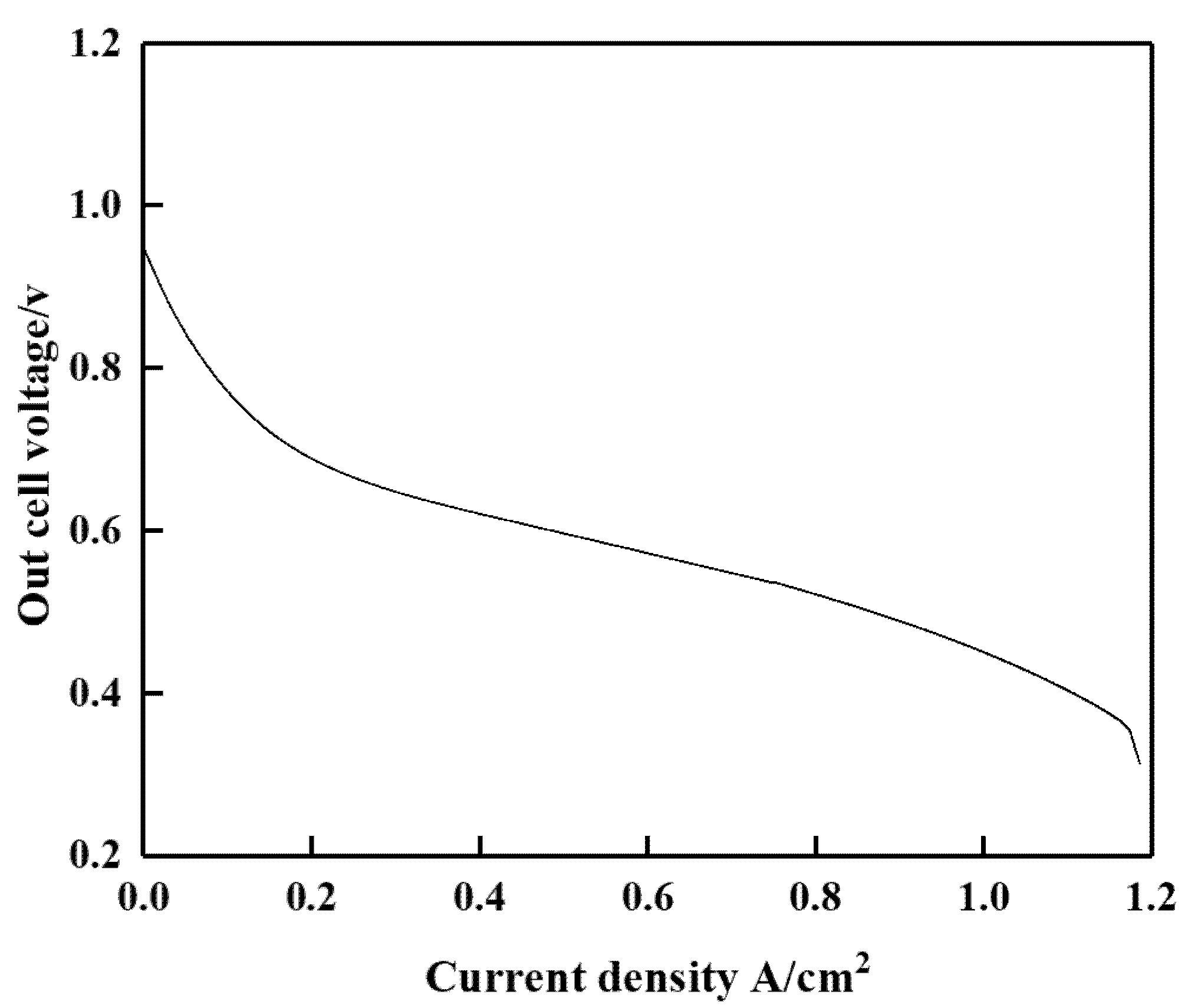
The chemical reaction that occurs in the fuel cell is the reverse reaction of the electrolysis of water. The hydrogen fuel cell system is not limited by the Carnot cycle, with a theoretical efficiency up to 90%. In this paper, the model [22] used mathematical formulas to describe the fuel cell stack and accessories, which include the air compressor, cathode and anode air supply manifold, humidifiers, coolers and return manifold, etc. The model was built using MATLAB/SIMULINK (MathWorks, Natick, MA, USA) to simulate the operation of the fuel cell system process. For calculation purposes, the model assumed that the temperature of the fuel cell was in an ideal state, without considering the impact of the electric double layer. Furthermore, all of the gases were assumed to be ideal gases. The electrochemical reaction was calculated in detail in the stack model. The parameters of the fuel cell in the model are presented in Table 1. Table 2 shows the simulated fuel cell failure states and the values set for the failures [23,24,25]. Figure 2 shows the PEMFC system block diagram. Figure 3 shows the polarization curve diagram of the fuel cell model without failure. As the current density increased, the output voltage of the fuel cell experienced an accelerated decline, a gradual decline and an accelerated decline. When the current density is low, the output voltage of the stack is determined by the activation polarization loss. As the current density increases, the influence of ohmic polarization loss increases. When the current density is high, the output voltage is mainly affected by the concentration loss. Generally speaking, the polarization shows the peculiarity of the fuel cell. At the same current, the lower the voltage loss, the better the peculiarity of the fuel cell.
Equations (18)–(27) are used to simulate faults 1 to 8. The compressor motor torque calculation is carried out using the following Equation (18):
where is the torque constant of the motor, is the electrical constant of the motor, is the mechanical efficiency of the motor, is the input voltage of the motor and is the speed of the air compressor. is used to simulate the local change in torque caused by the friction in the internal components of the compressor at fault 1. is used to simulate the torque change of fault 2 caused by the motor overheating.
The cathode outlet airflow is calculated as follows:
where is a cathode outlet orifice constant, is the cathode pressure, is the return manifold pressure. The increase in the cathode outlet aperture constant is used to simulate the gas flow caused by the excessive water in the cathode in fault 3.
The mass flow rate at the outlet of the gas supply manifold is calculated as follows:
where is the outlet orifice constant of the gas supply manifold, is the return manifold pressure and is the cathode pressure. The increase in the outlet orifice constant of the gas supply manifold can simulate the decrease in gas flow caused by gas leakage in fault 4.
Fault 5, the temperature control of the cooler is realized by directly setting the temperature change.
where is the initial temperature value set by the cooler, is the temperature change of the cooler and is the actual temperature value of the cooler.
Fault 6, the humidity control failure of the humidifier, is realized by directly setting the humidity change.
where is the humidity initially set by the humidifier, is the increase in the humidity change and is the actual humidity value of the humidifier.
Fault 7, the internal temperature control fault of the stack, is set by changing the temperature.
Fault 8, the output pipeline gas leakage fault is simulated by multiplying the output pipeline flow rate by a coefficient , which is greater than 0 and less than 1:
4. Fault Diagnosis of Fuel Cell System
Gaussian noise with a variance of 1 is added to the step dynamic current input to simulate the fault noise of the fuel cell under actual operating conditions [23]. Under dynamic conditions, faults 1 to 8 were simulated using the method mentioned in Section 3 in the model. The 12 parameters in the fuel cell model were used as variable fault diagnosis parameters, including fuel cell voltage, speed of the air compressor, air compressor outlet pressure, air compressor motor current, compressor output flow, hydrogen inlet pressure, air inlet pressure, over-oxygen rate, main supply pipe output temperature, supply pipe output pressure, outlet manifold flow and outlet manifold gas pressure.
Noise was added to the fuel cell model and the data samples of 12 diagnostic parameters in nine states were taken as the original samples. The simulations were carried out by MATLAB 2018a. The ELM and SVM algorithms are written in ‘.m’ files.
4.1. ELM Fault Classification Method
The 400 s data obtained from the simulation were used as the data set. First, the data set needed to be normalized. Using principal component analysis, the normalized 12-dimensional matrix was reduced to a 3-dimensional one with a cumulative contribution rate of over 85%. Finally, the model trained by ELM was trained to test the precision of the data fault classification. A flowchart of the ELM fault diagnosis method is shown in Figure 4.
The fault diagnosis strategy proposed in this paper is based on the fuel cell mechanism model, with eight common faults. The change values of 12 diagnostic variables over time were used as the original data set. The 400 s data obtained from the simulation were used as the data set. First, the data set needed to be normalized. The formula is shown in Equation (28).
In Equation (28), i = 1, 2,…, N, N is the number of data, is the selected diagnostic variable, and is the normalized variable.
In order to reduce computation and extract eigenvalues, the principal component analysis method needs to be used to reduce the dimensionality of the data and extract features. Data dimensionality reduction can reduce computational complexity. The process of feature extraction can obtain useful features for diagnosis. When the dimension is reduced to four dimensions, the matrix contribution rate can reach more than 85% through calculation.
When using ELM to build a fault classification model, the training set is made to have 350 samples, and the test set is made to have 50 samples. The model trained using the ELM algorithm is used to classify the test set to complete the fault diagnosis.
The classification result of the fault diagnosis method based on the extreme learning machine is shown in Figure 5. In Figure 5, ‘0’ means fault 0, ‘1’ means fault 1, ‘2’ means fault 2, ‘3’ means fault 3, ‘4’ means fault 4, ‘5’ means fault 5, ‘6’ means fault 6, ‘7’ means fault 7 and ‘8’ means fault 8. The average accuracy rate of the extreme learning machine model for fault classification on the test set was 78.76% and the time of algorithm classification was 0.36 s.
4.2. Support Vector Machine Fault Classification Method
The same data set was input into the support vector machine. The training set contained 350 samples and the test set contained 50 samples. A flow chart of the use of the support vector machine as a fault diagnosis method is shown in Figure 6. In the support vector machine algorithm, the optimal values of the parameters ‘c’ and ‘g’ of the kernel function REF obtained via the cross-validation method were 256 and 0.0039, respectively.
Inputting the 50 test samples into the model, the test result using the support vector machine classification strategy is shown in Figure 7. In Figure 7, ‘0’ means fault 0, ‘1’ means fault 1, ‘2’ means fault 2, ‘3’ means fault 3, ‘4’ means fault 4, ‘5’ means fault 5, ‘6’ means fault 6, ‘7’ means fault 7 and ‘8’ means fault 8. The average accuracy of the test set results was 83.33%, and the time of algorithm classification was 0.41 s.
The fault classification model trained using the extreme learning machine algorithm showed a higher average accuracy and a shorter time than the fault classification trained using the support vector machine algorithm. However, the fault diagnosis needs to be more accurate during the driving process.
4.3. GA-SVM Fault Classification Method
The genetic algorithm is an algorithm based on the principle of genetics. The algorithm uses three operators to perform genetic operations, which including selection, crossover and mutation. Through the evolution and development of the entire population under the principle of survival of the fittest, the optimal state is finally obtained.
The GA is used to find the most appropriate value of the kernel function ‘g’ and the residual ‘c’ in the SVM. The training set is made to have 350 samples, and the test set is made to have 50 samples. A flowchart of the GA-SVM fault diagnosis method is shown in Figure 8. The number of iterations was selected as 100, the maximum number of population was selected as 50, the value interval of parameter ‘c’ was limited to [0, 100], and the value interval of parameter ‘g’ was limited to [0, 100]. Finally, the optimal value of the parameter ‘c’ was calculated to be 3.47, and the optimal value of the parameter ‘g’ was 0.88.
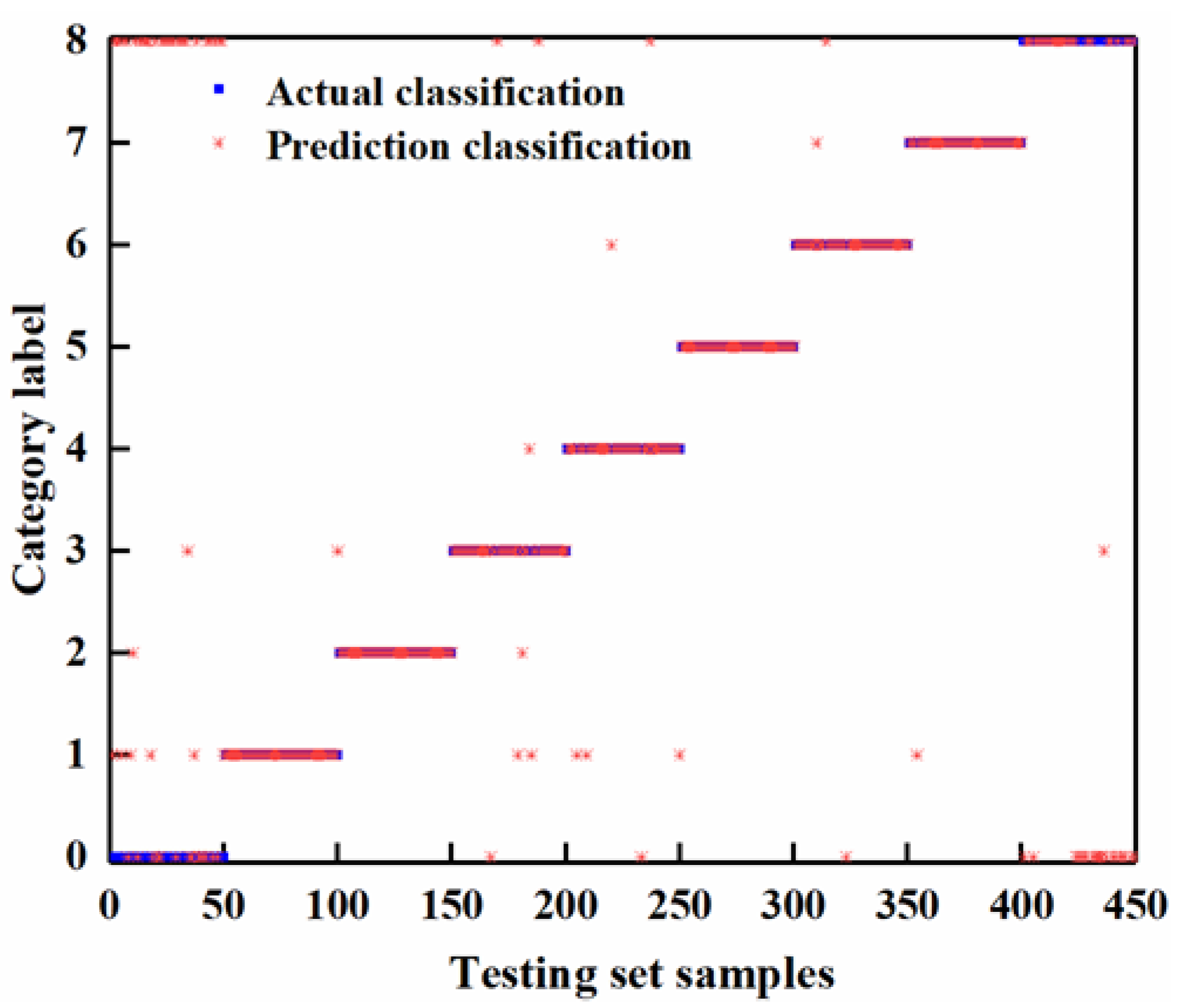
The classification results of the SVM optimized using the genetic algorithm are shown in Figure 9. The accuracy of the test set was 94%, and the time of fault classification was 0.18 s. It can be clearly seen from the test results that the support vector machine optimized using the genetic algorithm showed the highest accuracy in terms of fault classification.
4.4. Comparison and Analysis of Failure Results
By inputting the same fault data set, the extreme learning machine, support vector machine and genetic algorithm optimization support vector machine were used for fault diagnosis. The accuracy of the three classification algorithms is shown in Table 3. The time used by three algorithms is shown in Table 4.
A shown in Table 3, the test accuracy based on the two fuel cell fault diagnosis methods of SVM and ELM had nothing to do with the fault type. The results for different fault types were not the same. The fault diagnosis based on the ELM algorithm showed a high classification accuracy for fault 1, fault 2, fault 4 and fault 6. The fault diagnosis based on the SVM algorithm showed a very high accuracy for fault 0, fault 3, fault 4, fault 7 and fault 8. However, the fault accuracy rate based on ELM was higher than that of SVM. The GA-SVM-based method showed the highest classification accuracy rate for various faults, which shows that the support vector machine classification algorithm based on genetic algorithm optimization improved the classification accuracy obviously. Through careful observation, it can be seen that the GA-SVM algorithm showed a lower recognition accuracy than the SVM algorithm in the fault-free state. This may be due to the fact that the data characteristics of the fault 0 state were similar to those of fault 5 after optimization.
Based on Table 4, the use of the ELM algorithm takes a shorter test time than SVM. The classification speed of ELM was 12% higher than that of SVM. The time of the GA-SVM algorithm classification was 0.18 s, and the classification accuracy was significantly improved.
5. Conclusions
In order to identify faults in fuel cells, PEMFC, ELM and SVM approaches were used to train a classification model. The results showed that the ELM algorithm had a shorter classification time and the SVM algorithm had a higher average classification accuracy. However, the accuracy of the two algorithms was less than 80%. In order to enhance the efficiency of fault classification, a genetic algorithm was used to optimize the support vector machine. The accuracy rate reached 94% after optimization.
In this paper we used the models to diagnose 8 single faults. At present, little research work has been completed on simultaneous fault diagnosis. As a next step, the study of diagnosis methods when two or more faults occur in a fuel cell system will be conducted, based on this article.
Author Contributions
Conceptualization, methodology, validation, W.H.; resources, W.L.; data curation, W.L. writing—original draft preparation, W.H.; writing—review and editing, C.S., Q.R. and G.G. All authors have read and agreed to the published version of the manuscript.
Funding
This research is funded by the Key Research and Development Program of Guangdong Province (No. 2019B090909001), the Beijing laboratory construction—Beijing Laboratory for New Energy Vehicles (PXM2020_014224 _000065), the Supplementary and Supportive Project for Teachers at Beijing Information Science and Technology University (2018–2020) (5029011103), the Promoting connotation development of university “Information +” at Beijing Information Science and Technology University (2019) (5121911012), the Technology program of Beijing Municipal Education Commission (KM201911232023).
Institutional Review Board Statement
Not applicable.
Informed Consent Statement
Not applicable.
Data Availability Statement
The data that support this manuscript are available from Weier Li upon reasonable request.
Conflicts of Interest
The authors declare no conflict of interest.
Abbreviations
| PEMFC | Proton exchange membrane fuel cell |
| SOFC | Solid oxide fuel cell |
| His | Health indices |
| EIA-PSO | Effective informed adaptive particle swarm optimization |
| DS | Dempster-Shafer |
| HSMMs | Hidden semi-Markov models |
| SVM | Support vector machine |
| LS-SVM | Least squares support vector machine |
| ELM | Extreme learning machine |
| GA | Genetic algorithm |
| GA-SVM | Genetic algorithm support vector machine |
| BPNN | Back propagation neural network |
References
- Hissel, D.; Candusso, D.; Harel, F. Fuzzy-clustering durability diagnosis of polymer electrolyte fuel cells dedicated to transportation applications. IEEE Trans. Veh. Technol. 2007, 56, 2414–2420. [Google Scholar] [CrossRef]
- Chen, H.; Zhang, Z.; Guan, C. Optimization of sizing and frequency control in battery/supercapacitor hybrid energy storage system for fuel cell ship. Energy 2020, 197, 117285. [Google Scholar] [CrossRef]
- Simon Araya, S.; Zhou, F.; Lennart Sahlin, S.; Thomas, S.; Jeppesen, C.; Knudsen Kær, S. Fault Characterization of a Proton Exchange Membrane Fuel Cell Stack. Energies 2019, 12, 152. [Google Scholar] [CrossRef] [Green Version]
- Won, J.; Oh, H.; Hong, J.; Kim, M.; Lee, W.Y.; Choi, Y.Y.; Han, S.B. Hybrid diagnosis method for initial faults of air supply systems in proton exchange membrane fuel cells. Renew. Energy 2021, 180, 343–352. [Google Scholar] [CrossRef]
- Liu, J.; Luo, W.; Yang, X.; Wu, L. Robust model-based fault diagnosis for PEM fuel cell air-feed system. IEEE Trans. Ind. Electron. 2016, 66, 3261–3270. [Google Scholar] [CrossRef] [Green Version]
- Zuo, B.; Zhang, Z.; Cheng, J.; Huo, W.; Zhong, Z.; Wang, Z. Data-driven flooding fault diagnosis method for proton-exchange membrane fuel cells using deep learning technologies. Energy Convers. Manag. 2022, 251, 115004. [Google Scholar] [CrossRef]
- Zhou, S.; Jin, J.; Wei, Y. Research on Online Diagnosis Method of Fuel Cell Centrifugal Air Compressor Surge Fault. Energies 2021, 14, 3071. [Google Scholar] [CrossRef]
- Lim, I.S.; Park, J.Y.; Choi, E.J.; Kim, M.S. Efficient fault diagnosis method of PEMFC thermal management system for various current densities. Int. J. Hydrogen Energy 2021, 46, 2543–2554. [Google Scholar] [CrossRef]
- Zhuo, S.; Gaillard, A.; Xu, L.; Liu, C.; Paire, D.; Gao, F. An Observer-Based Switch Open-Circuit Fault Diagnosis of DC–DC Converter for Fuel Cell Application. IEEE Trans. Ind. Appl. 2020, 56, 3159–3167. [Google Scholar] [CrossRef]
- Shao, M.; Zhu, X.J. An artificial neural network ensemble method for fault diagnosis of proton exchange membrane fuel cell system. Energy 2014, 67, 268–275. [Google Scholar] [CrossRef]
- Li, Q.; Chen, W.R.; Liu, Z.X.; Guo, A.; Huang, J. Nonlinear multivariable modeling of locomotive proton exchange membrane fuel cell system. Int. J. Hydrogen Energy 2014, 39, 13777–13786. [Google Scholar] [CrossRef]
- Liu, J.; Li, Q.; Chen, W.; Yan, Y.; Wang, X. A fast fault diagnosis method of the PEMFC system based on extreme learning machine and dempster–shafer evidence theory. IEEE Trans. Transp. Electrif. 2019, 5, 271–284. [Google Scholar] [CrossRef]
- Wu, X.J.; Ye, Q.W. Fault diagnosis and prognostic of solid oxide fuel cells. J. Power Sources 2016, 321, 47–56. [Google Scholar] [CrossRef]
- Zhao, X.; Xu, L.F.; Li, J.Q.; Fang, C.; Ouyang, M.G. Faults diagnosis for PEM fuel cell system based on multi-sensor signals and principle component analysis method. Int. J. Hydrogen Energy 2017, 42, 18524–18531. [Google Scholar] [CrossRef]
- Djeziri, M.; Djedidi, O.; Benmoussa, S.; Bendahan, M.; Seguin, J.L. Failure Prognosis Based on Relevant Measurements Identification and Data-Driven Trend-Modeling: Application to a Fuel Cell System. Processes 2021, 9, 328. [Google Scholar] [CrossRef]
- Du, R.B.; Wei, X.Z.; Wang, X.Y.; Chen, S.Q.; Yuan, H.; Dai, H.F.; Ming, P.W. A fault diagnosis model for proton exchange membrane fuel cell based on impedance identification with differential evolution algorithm. Int. J. Hydrogen Energy 2021, 46, 38795–38808. [Google Scholar] [CrossRef]
- Zhang, X.; Guo, X. Fault diagnosis of proton exchange membrane fuel cell system of tram based on information fusion and deep learning. Int. J. Hydrogen Energy 2021, 46, 30828–30840. [Google Scholar] [CrossRef]
- Gao, Z.; Cecati, C.; Ding, S.X. A Survey of Fault Diagnosis and Fault-Tolerant Techniques—Part I: Fault Diagnosis With Model-Based and Signal-Based Approaches. IEEE Trans. Ind. Electron. 2015, 62, 3757–3767. [Google Scholar] [CrossRef] [Green Version]
- Gao, Z.; Cecati, C.; Ding, S.X. A Survey of Fault Diagnosis and Fault-Tolerant Techniques—Part II: Fault Diagnosis With Knowledge-Based and Hybrid/Active Approaches. IEEE Trans. Ind. Electron. 2015, 62, 3768–3774. [Google Scholar] [CrossRef]
- Li, Y.; Zeng, Y.J.; Qing, Y.Y.; Huang, G.B. Learning local discriminative representations via extreme learning machine for machine fault diagnosis. Neurocomputing 2020, 409, 275–285. [Google Scholar] [CrossRef]
- Yuan, X.; Liu, Z.; Miao, Z.; Zhao, Z.; Zhou, F.; Song, Y. Fault diagnosis of analog circuits based on IH-PSO optimized support vector machine. IEEE Access 2019, 7, 137945–137958. [Google Scholar] [CrossRef]
- Pukrushpan, J.T.; Stefanopoulou, A.; Peng, H. Control of Fuel Cell Power Systems: Principles, Modeling, Analysis and Feedback Design; Springer: Berlin/Heidelberg, Germany, 2004. [Google Scholar]
- Escobet, A.; Nebot, A.; Mugica, F. PEM fuel cell fault diagnosis via a hybrid methodology based on fuzzy and pattern recognition techniques. Eng. Appl. Artif. Intell. 2014, 36, 40–53. [Google Scholar] [CrossRef] [Green Version]
- Rosich, A.; Sarrate, R.; Nejjari, F. On-line model-based fault detection and isolation for PEM fuel cell stack systems. Appl. Math. Model. 2014, 38, 2744–2757. [Google Scholar] [CrossRef]
- Kamal, M.; Yu, D.; Yu, D.; Yu, D. Fault detection and isolation for PEM fuel cell stack with independent RBF model. Eng. Appl. Artif. Intell. 2014, 28, 52–63. [Google Scholar] [CrossRef]
- Liu, J.W.; Li, Q.; Chen, W.R.; Yan, Y.; Wang, X.T. Research on the fault diagnosis of a polymer electrolyte membrane fuel cell system. Energies 2020, 13, 2531. [Google Scholar]
Figure 1.
Network structure diagram of an ELM.

Figure 2.
PEMFC system block diagram. Reprinted with permission from Springer-Verlag London 2004, 2021 [22].
Figure 2.
PEMFC system block diagram. Reprinted with permission from Springer-Verlag London 2004, 2021 [22].

Figure 3.
The polarization curve of the fuel cell model.

Figure 4.
Flow diagram of ELM diagnosis process.

Figure 5.
Predictive classification results of ELM algorithm.

Figure 6.
Flow diagram of the SVM diagnosis process.

Figure 7.
Predictive classification results of the SVM algorithm.

Figure 8.
Flow diagram of the GA-SVM diagnosis process.

Figure 9.
Predictive classification results of the GA-SVM algorithm.


Table 1.
Fuel cell model parameters. Developed with permission from Springer-Verlag London 2004, 2021 [22].
Table 1.
Fuel cell model parameters. Developed with permission from Springer-Verlag London 2004, 2021 [22].
| Symbol | Parameter | Value |
|---|---|---|
| Effective activation area | Afc | 280 cm2 |
| Number of cells | n | 381 |
| Anode volume | Van | 0.005 m3 |
| Cathode volume | Vca | 0.01 m3 |
| Membrane thickness | tm | 0.01275 cm |
| Compressor diameter | dc | 0.2286 m |
| Compressor and motor inertia | JCP | 5 × 10⁻⁵ kg × m2 |
| Compressor motor circuit resistance | Rcm | 1.2 Ω |
| Motor electric constant | kv | 0.0153 V/(rad/s) |
| Motor torque constant | kt | 0.225 N × m/A |
| Motor mechanical efficiency | ƞcm | 98% |
| Supply manifold volume | Vsm | 0.02 m3 |
| Supply manifold outlet orifice constant | Ksm,out | 0.36293 × 10⁻⁵ kg/(s × Pa) |
| Return manifold volume | Vrm | 0.005 m3 |
| Motor electric constant | kv | 0.0153 V/(rad/s) |
| Motor torque constant | kt | 0.225 N × m/A |
Table 2.
Faults in the PEM fuel cell simulator model. Developed from [26].
Table 2.
Faults in the PEM fuel cell simulator model. Developed from [26].
| Fault ID | Fault Description | Type | Magnitude |
|---|---|---|---|
| Fault 0 | Normal state | Parametric unchanged | 0 |
| Fault 1 | Sudden increase in friction of compressor mechanical parts | Abrupt change | Flow coefficient increased by 10% |
| Fault 2 | The temperature of the compressor motor is too high | Abrupt change | Internal resistance increased by 100% |
| Fault 3 | Flooding failure in stack | Abrupt change | Reduce water flow by 50% |
| Fault 4 | Air leak in the air supply manifold | Abrupt change | Reduce air flow by 50% |
| Fault 5 | The cooler temperature control failure | Gradual change | Temperature increment of 10 K |
| Fault 6 | The humidifier control failure | Gradual change | Humidity increase by 20% |
| Fault 7 | The stack temperature control failure | Gradual change | Temperature increment of 10 K |
| Fault 8 | Air leak in the outlet manifold | Abrupt change | Reduce gas flow by 30% |
Table 3.
Fault diagnosis accuracy rates of different classification methods.
| Classification | Fault 0 | Fault 1 | Fault 2 | Fault 3 | Fault 4 | Fault 5 | Fault 6 | Fault 7 | Fault 8 | Average |
|---|---|---|---|---|---|---|---|---|---|---|
| ELM | 76% | 68% | 86% | 78% | 84% | 90% | 66% | 80% | 80% | 78.67% |
| SVM | 28% | 98% | 100% | 86% | 88% | 100% | 94% | 98% | 58% | 83.33% |
| GA-SVM | 86% | 88% | 100% | 100% | 100% | 86% | 100% | 100% | 84% | 98% |
Table 4.
Fault diagnosis times of different classification methods.
| Classification | Time |
|---|---|
| ELM | 0.36 s |
| SVM | 0.41 s |
| GA-SVM | 0.18 s |
Publisher’s Note: MDPI stays neutral with regard to jurisdictional claims in published maps and institutional affiliations. |
© 2022 by the authors. Licensee MDPI, Basel, Switzerland. This article is an open access article distributed under the terms and conditions of the Creative Commons Attribution (CC BY) license (https://creativecommons.org/licenses/by/4.0/).
Share and Cite
MDPI and ACS Style
Huo, W.; Li, W.; Sun, C.; Ren, Q.; Gong, G. Research on Fuel Cell Fault Diagnosis Based on Genetic Algorithm Optimization of Support Vector Machine. Energies 2022, 15, 2294. https://doi.org/10.3390/en15062294
AMA Style
Huo W, Li W, Sun C, Ren Q, Gong G. Research on Fuel Cell Fault Diagnosis Based on Genetic Algorithm Optimization of Support Vector Machine. Energies. 2022; 15(6):2294. https://doi.org/10.3390/en15062294
Chicago/Turabian StyleHuo, Weiwei, Weier Li, Chao Sun, Qiang Ren, and Guoqing Gong. 2022. "Research on Fuel Cell Fault Diagnosis Based on Genetic Algorithm Optimization of Support Vector Machine" Energies 15, no. 6: 2294. https://doi.org/10.3390/en15062294
Note that from the first issue of 2016, this journal uses article numbers instead of page numbers. See further details here.