
Discussion of Wind Turbine Performance Based on SCADA Data and Multiple Test Case Analysis


1
Department of Engineering, University of Perugia, Via G. Duranti 93, 06125 Perugia, Italy
2
Centre for Life-Cycle Engineering and Management (CLEM), School of Aerospace Transport and Manufacturing, Cranfield University, Bedford MK43 0AL, UK
3
ENGIE Italia, Via Chiese, 20126 Milano, Italy
*
Author to whom correspondence should be addressed.
Energies 2022, 15(15), 5343; https://doi.org/10.3390/en15155343
Submission received: 4 July 2022
/
Revised: 18 July 2022
/
Accepted: 22 July 2022
/
Published: 22 July 2022
(This article belongs to the Special Issue Decision-Making Systems in Power System Planning and Operation in the Presence of High Shares of Renewable Energies)
Abstract
:This work is devoted to the formulation of innovative SCADA-based methods for wind turbine performance analysis and interpretation. The work is organized as an academia–industry collaboration: three test cases are analyzed, two with hydraulic pitch control (Vestas V90 and V100) and one with electric pitch control (Senvion MM92). The investigation is based on the method of bins, on a polynomial regression applied to operation curves that have never been analyzed in detail in the literature before, and on correlation and causality analysis. A key point is the analysis of measurement channels related to the blade pitch control and to the rotor: pitch manifold pressure, pitch piston traveled distance and tower vibrations for the hydraulic pitch wind turbines, and blade pitch current for the electric pitch wind turbines. The main result of this study is that cases of noticeable under-performance are observed for the hydraulic pitch wind turbines, which are associated with pitch pressure decrease in time for one case and to suspected rotor unbalance for another case. On the other way round, the behavior of the rotational speed and blade pitch curves is homogeneous and stable for the wind turbines electrically controlled. Summarizing, the evidence collected in this work identifies the hydraulic pitch as a sensible component of the wind turbine that should be monitored cautiously because it is likely associated with performance decline with age.
1. Introduction
Horizontal-axis wind turbines constitute a mature and the most promising renewable energy technology worldwide [1,2]. Therefore, there is an impressive amount of wind turbines operating in the field since a certain number of years, reaching the end of the theoretical lifetime expectancy. For example, in [3], it was reported that in 2020, 28% of wind turbines installed in Europe were older than 15 years of age, with peaks in the order of 50% in Spain, Germany, and Denmark.
This matter of fact motivates a recent deeper attention to the analysis and the interpretation of wind turbine performance, which is in general complicated because there are issues related with quantity and quality of nacelle anemometer data [4,5]. It is generally expected that the performance of whatever technical system declines with age [6,7] and the growing amount of aged operating wind turbines poses the issue of wind turbine performance analysis with a major urgency. Nevertheless, it is not rare that wind turbines might also under-perform in the first years of operation, and therefore the analysis is encouraged throughout all the wind farm lifetime.
The literature about wind turbine performance decline with age provides order of magnitude estimates of expected trends, and is useful to summarize briefly. Basing on the analysis of cumulative data, in [8], an average decline of per year is estimated for UK wind farms. The estimate provided by [9], with a similar method, is lower. The studies in [10,11] deal with the analysis of a vast set of wind farms sited, respectively, in Germany and the U.S.: from those works, the hypothesis is supported that the older the wind turbine technology, the higher the average performance decline rate with age. In particular, in [11], it is reported that wind farms installed before (respectively, after) the year 2008 averagely lose 0.63% (respectively, 0.17%) per year. In [12], cumulative data of offshore wind farms in UK are analyzed and the conclusion is that the technical efficiency does not decline with age.
Recently, another approach has been developed in the literature for the estimation of performance decline with age, which is based on employing detailed information (SCADA data) [13,14]. The studies in [15,16,17,18] deal with the Vestas V52 wind turbine: in particular, for one considered test case, a remarkable performance decline with age is observed in the form of diminished extracted power for a given generator speed. In [19], data of 2 MW wind turbines with electrical pitch control are analyzed, and the main result is that the performance worsening with age is very limited. These results constitute the nutshell from which the present work moves: actually, through comparative test case analysis, it is meaningful to inquire if wind turbine under-performance is more a matter of technology type rather than size or age.
The above remarks lead to the argument that a space–time approach based on the whole wind farm [20,21] is useful for the interpretation of wind turbine performance. Given the fact that wind turbines are typically grouped in clusters, the behavior of a wind turbine can be compared against the nearby ones in the same period or against itself in different periods. Evidently, given the non-stationary conditions to which wind turbines are subjected, this calls for devoted data analysis techniques, which have also been developed at least in part in previous studies like [15,16,21].
On these grounds, the objective of the present study is providing innovative SCADA data analyses, which are useful for the interpretation of wind turbine performance. In particular, a turning point is the selection of what SCADA measurements are employed. Actually, as long as wind turbine technology evolves, more and more measurements become available to the end users of SCADA control systems: environmental variables, working parameters, sub-component temperatures, voltages and currents, tower vibrations, internal pressures and so on. In the scientific literature and in the industry practice, this information is in general under-exploited.
The work is organized as a collaboration between academia and wind energy utility companies operating in Italy (ENGIE Italia and Lucky Wind). The study is based on a comparative test case discussion: in particular, data from three wind farms have been analyzed. The selected wind turbines have 2 MW of rated power each: one test case wind farm features Senvion MM92 wind turbines, having electric pitch control, and the other two wind farms are composed of Vestas V90 and V100 wind turbines, having hydraulic pitch control. For the hydraulic pitch test cases, measurements of pitch manifold pressure, pitch piston traveled distance and tower vibrations are analyzed, while for the electrically controlled wind turbine the blade pitch current is included in the analysis. To the best of the authors’ knowledge, there are no studies in the literature that systematically address these types of SCADA-based measurements in relation to the performance of the wind turbines: this constitutes a key innovative aspect of the present study.
The general point of view of this work is that it is prohibitive to identify the root cause of an under-performance using SCADA data, but it is possible to collect meaningful clues, which can support coherent hypotheses and exclude contradictory ones. The results of this study indicate that the information related to the hydraulic pitch system [22,23] is particularly useful in order to interpret wind turbine performance. In particular, the under-performance of one selected test case is observed to be associated to a decrease of the pitch manifold block pressure. For the other hydraulically controlled test case, a noticeable difference in the power–pitch and power–pitch piston distance curves occurs and, furthermore, anomalous tower vibrations are individuated, which can be likely be interpreted as due to an unbalanced rotor case. A more general lesson of this study is that the analysis of the correlation between features is simplistic for wind turbine monitoring: actually, variables with moderate or even low correlation with the power might provide meaningful insight on the wind turbine behavior.
2. The Test Cases and the Data Sets
Three test case wind farms are considered in this study:
- WF1 is composed of 4 Vestas V100 wind turbines;
- WF2 is composed of 7 Vestas V90 wind turbine;
- WF3 is composed of 6 Senvion MM92 wind turbines.
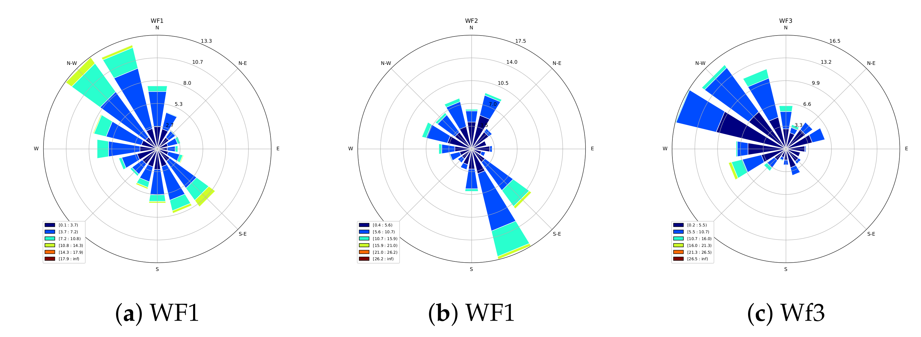
WF1 is owned by the Italian utility company Lucky Wind and WF2 and WF3 are owned by ENGIE Italia. All the wind turbines are sited in southern Italy on quite gentle terrains, and the average turbulence intensity is not exceptional. Sample annual wind roses are reported in Figure 1: there are no evident variations in the wind speed and intensity distribution from year to year. The inter-distance between the wind turbines is quite high (order of at least 7 rotor diameters) and in any case, the operation under wake is quite rare for the all the test case wind farms. Based on these considerations, there are arguments supporting that the environments in which the wind farms are sited are not so peculiar or different as to justify the performance scenario, which will be discussed in Section 4.
For the discussion of Section 4, it is meaningful to clarify that the wind turbines are equipped with doubly-fed induction generators from a few producers, which are the same for the three test cases. The rationale for the selection of these test cases is the following: the wind turbines of WF3 have electric pitch control, while those of WF1 and WF2 have hydraulic pitch control. In WF1 and WF2, there are under-performance issues, having different time and space features which will be discussed in detail in Section 4.
Coherently with the type of technology and the age of each wind turbine model, the available measurements are different for the various test cases. The most important measurement channels are present in the SCADA system of all the test cases and are the following:
- Wind speed v (m/s);
- Active power P (kW);
- Generator speed (rpm);
- Blade pitch ();
- Run time counter (s).
Other measurement channels have been selected peculiarly for each test case, depending on the data availability and the technology: these are indicated in Table 1, together with the fundamental features of the wind turbines and the data sets selected for the analysis. It should be pointed out that the data available for the analysis go from the installation date (in 2016) to the year 2021 for WF1 and from the years 2010 to 2021 for WF2 and WF3. The selection of the data sets (indicated in Table 1) has been done in order to highlight the space–time behavior that has been considered relevant for the discussion of the study.
The measurements are acquired by the typical industrial SCADA systems employed in wind turbine technology, with a sampling time that can reach the Hz. Subsequently, the data are averaged with an averaging time of ten minutes and are made available to the end-user: these data have been employed for the present work. No information about the instrumental uncertainty has been provided: nevertheless, it is important to notice that, being the employed data averaged on a ten minutes basis, the statistical uncertainty is expected to be more relevant than the instrumental.
The same procedure of data pre-processing has been applied to all the data sets for all the test cases. It goes as follows:
- Request that the wind turbine is productive: s.
- Filter out limitations due to grid requirements. This can be achieved by eliminating the outliers with respect to the average wind speed–blade pitch curve: a threshold of has been employed for this study. The rationale is that a wind turbine gets derated by forcing it to pitch anomalously. This method is practical, but for an in-depth analysis of outliers devoted methods could be employed [24].
- For under-performance analysis, request that the wind turbine is operating below rated speed, otherwise the performance monitoring would be trivial.
3. Methods
3.1. The Method of Bins
The method of bins for the analysis of operation curves is inspired by the well-established study of the power curve [25]. Actually, the International Electrotechnical Commission (IEC) [25] recommends to average power measurements upon grouping them in bins of 0.5 or 1 m/s. This concept is formulated through Equation (1):
The notation indicates that there are wind speed measurements for each i-th bin and that is j-th power output measurement in the i-th bin. Similarly, for each bin, the standard deviation of the measurements falling in each bin can be computed, which provides a meaningful indications of the data spread.
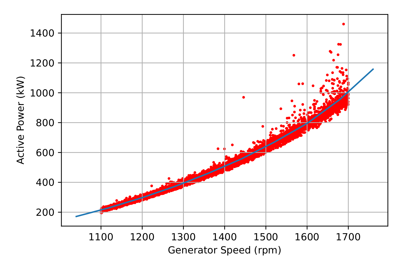
The method of bins is easy to generalize to whatever couple of quantities : it is sufficient to substitute with per bins of the quantity. A reasonable rule of thumb is considering intervals of in the order of 10% of the range that can assume. An example of a scattered and binned operation curve is reported in Figure 2.
The list of operation curves analyzed in this study is given in Table 2. For a space comparison, the curves are analyzed for a given period for all the fleet, while for a time comparison, the curves are analyzed for each wind turbine of interest for multiple periods.
3.2. Regression Analysis
The methods proposed in Section 3.1 are substantially qualitative, while for a deeper performance analysis quantitative results are needed. A space or time comparison necessarily passes through a data-driven regression for the curves of interest. Once a model has been trained basing on a reference data set for the input and the output , it can be employed for simulating the output given the input for the target data set: the residuals between measurements y and model estimates can be elaborated in order to perform the comparison between the reference and the target data set. Namely, the procedure goes as follows:
- Train the model using the reference data ;
- Feed the input x of the target data set to the model and simulate the output ;
- Compute the residuals between measurements and model estimates as in Equation (2):
- Estimate the average percentage difference between the reference and the target data set using Equation (3):
The data-driven model for the curves of interest has been selected to be as simple as possible. Basing on the literature about power curve analysis [26,27], a fifth-order polynomial has been adopted (Equation (4)), which is fitted to the training data using the Python library.
The space and time comparison is performed by selecting appropriately the reference and target data set, as indicated in Table 3. The selection of the reference data set for the time comparison and of the reference wind turbine for the space comparison depends on the objective. An intuitive, yet not mandatory, selection is picking one of the best performing wind turbines as reference for the space analysis and one of the earliest data sets as reference for the time analysis.
3.3. Correlation and Causation Analysis
The relation between the considered variables is analyzed quantitatively through the Pearson correlation coefficient and the Granger causality test [28].
The rationale for this twofold point of view is that it is not excluded that covariates having small correlation coefficient with the power have instead a relation with it, which can be considered statistically causal. Indeed, this is often the case as regards blade pitch and power of a wind turbine.
The Pearson correlation coefficient between the quantities x and y is defined in Equation (5):
where N is the number of measurements in the data set and and are the mean values of the x and y quantities in the data set. For the purposes of this study, y is selected to be the power P and the quantities of Table 1 are taken as x.
The Granger causality analysis [29] is based on the linear regression and inquires if the time series of a quantity x causally determines the time series of the y quantity. Lags could be included in the model, but this has been excluded in this analysis due to the 10-min averaging time of the SCADA-collected data set: therefore, the Granger analysis is pursued at an equal time. Additionally, hypothesis testing can be conducted to determine whether the result is statistically significant: significance values are calculated (p-values) based on the Fisher distribution, which define the probability of impact since the null hypothesis is true. When the p-value is below the specified level of significance ( in this work), the null hypothesis that x does not cause y is rejected.
For brevity, the above analysis will be reported for sample wind turbines, since the results are similar for all the fleet.
3.4. Pitch Efficiency Analysis
Inspired by the analysis in [30], which at present is the unique study in the literature expressly devoted to blade pitch aging assessment, in this work an analysis is replicated for the three test cases at disposal. In [30], it is argued that the aging of the blade pitch likely manifests as diminished efficiency in the capability of maintaining the rated power above rated speed. Therefore, in this study, a space–time comparison of the standard deviation of the power extracted above rated speed is performed, and it is inquired whether meaningful trends are visible.
4. Results
4.1. WF1
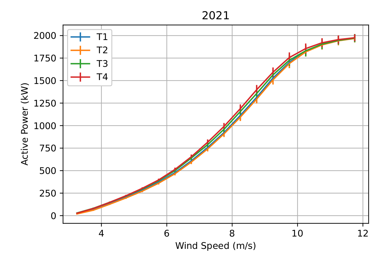
In Figure 3, the average power curve is reported for WF1 for the year 2021. From that figure, it arises that T4 is the best performing wind turbine of the farm and T2 is the worst. The performance difference between T4 and the other wind turbines is quantified through a space comparison based on the regression method explained in Section 3. The results are reported in Table 4 and it arises that wind turbine T2 has a performance lower with respect to T4 in the order of 8.7% averagely. Note that this quantity is referred to as the regime below rated power, and in percentage to the total production (including rated power) the performance shift would be lower.
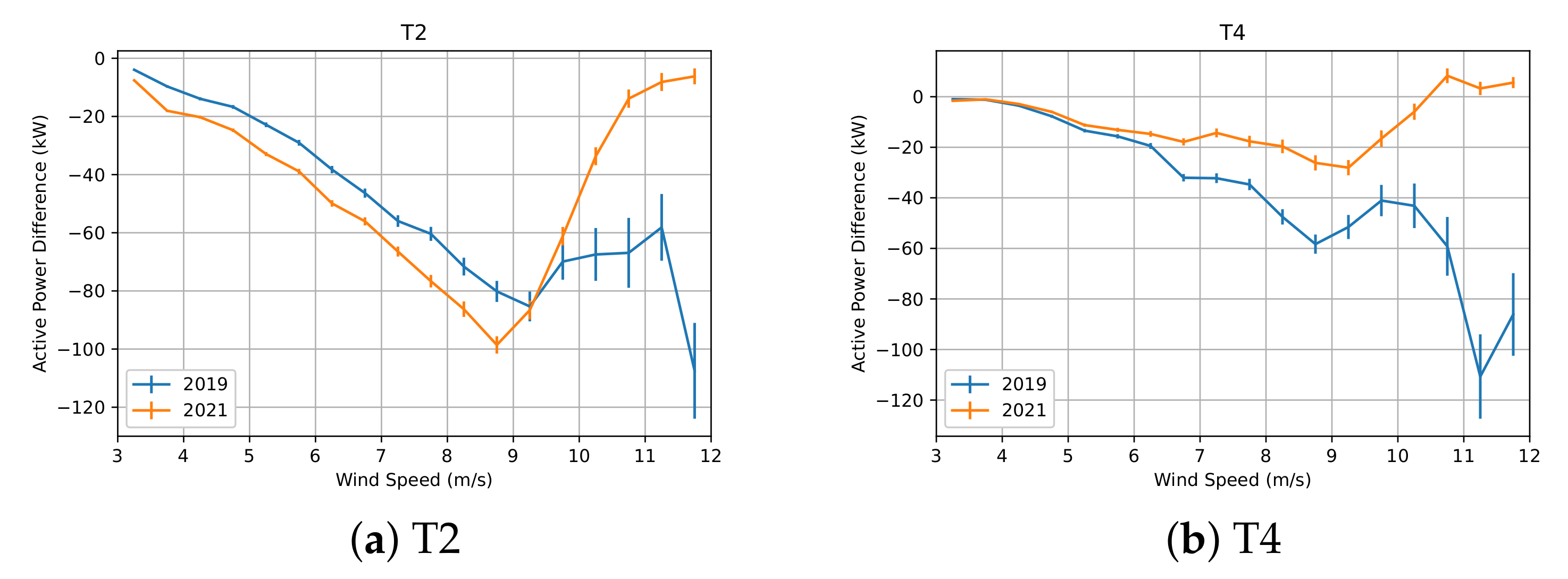
Given the above results, the following analysis is devoted to the comparison between T2 and T4. In Figure 4a, the difference between the average yearly power curve of the years 2019 and 2021 with respect to 2017 is reported for T2. From this figure, it arises that there is an evident decline from 2017 to 2019, and the situation is quite similar in 2021 with respect to 2017. The same kind of plot is reported in Figure 4b for wind turbine T4: a decline from 2017 to 2019 is evident, and there is a remarkable recovery in 2021 with respect to 2019. The statistical uncertainties are such that the behavior of the various years can be considered distinguishable.
Quantitative estimates confirming this picture are obtained through a time comparison based on the regression: the model is trained on the data from 2017 and used for simulating the 2019 and 2021 data, independently for wind turbines T2 and T4. The results are reported in Table 5: the percentage worsening from 2017 to 2019 is almost two times higher for T2 with respect to T4, and there is a recovery for T4 in 2021 with respect to 2019, while T2 keeps worsening and its performance is on average 9.7% lower in 2021 with respect to itself in 2017.
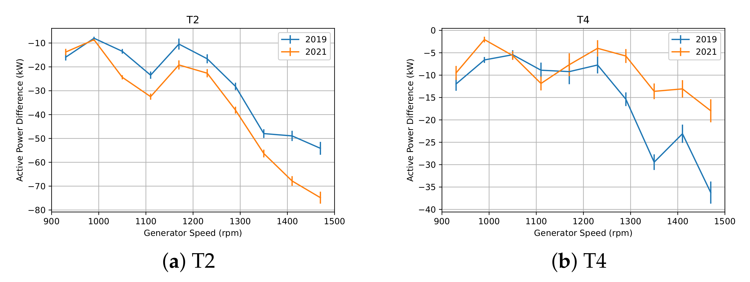
In order to exclude that the behavior observed in Figure 4a,b is biased by issues related to the wind speed measurement, the analysis continues with operation curves that do not employ the wind speed. In particular, in Figure 5a,b, the average generator speed–power curves are reported for T2 and T4 in the form of the difference between the years 2019 and 2021 with respect to the year 2017. Figure 5a,b substantially confirm the picture obtained from the power curve analysis of Figure 4a,b: the amount of power extracted for a given generator speed diminishes in time for T2 and diminishes for T4 in 2019, but then is at least partially recovered in 2021. Quantitative estimates of the performance trend are achieved by employing the same kind of procedure as for Table 5, applied to the generator speed–power curve. The results are collected in Table 6, with result qualitatively similar to Table 5.
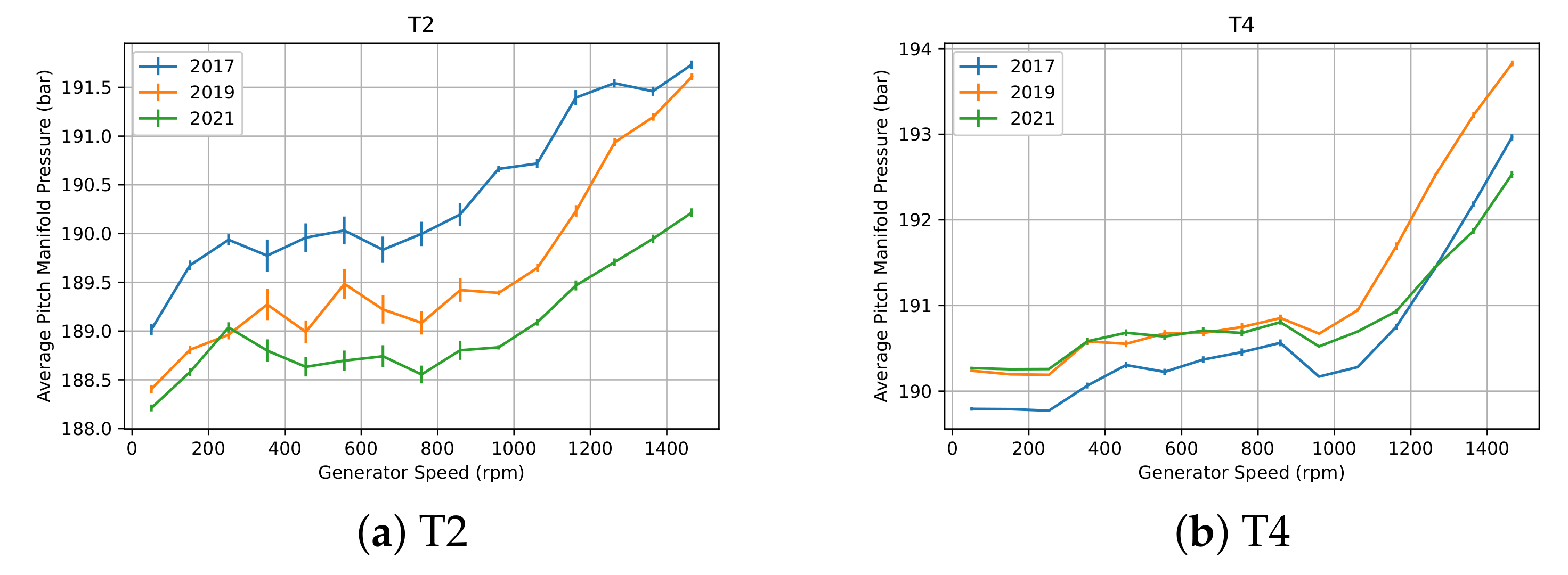
This kind of behavior has also been observed in [16] for a Vestas V52 wind turbine and in that work it has mainly been interpreted as due to the control of the rotational speed. In this work, given the possibility of comparing different test cases with different technology, the interpretation has been further elaborated and the hypothesis is that the performance decline can be ascribed to the hydraulic pitch control. Support for this hypothesis comes from Figure 6a,b, reporting the average pitch manifold pressure as a function of the generator speed for wind turbines T2 and T4 in the years 2017, 2019 and 2021. From Figure 6a, it arises that the pressure slightly diminishes in time for the given generator speed for wind turbine T2, while the opposite occurs for wind turbine T4 (Figure 6b). This can also be appreciated quantitatively from the regression analysis reported in Table 6, where it arises that a percentage decline of the average pitch manifold block pressure occurs for wind turbine T2 and not for T4.
The Pearson correlation coefficient between and P is 0.63. Although this correlation is moderate, the Granger analysis indicates causality with high statistical significance, since the achieved p-values are all in the order of or lower.
The above results can be interpreted with a line of reasoning similar to some considerations collected in [31], where it is argued that a different behavior of the blade pitch means a slightly different curve of the power coefficient as a function of the tip speed ratio. Furthermore, in [32], through numerical simulations it is argued that the pitch actuation rate is fundamental for determining an optimal control of the wind turbine and, on the other way round, a non-optimal pitch actuation rate leads exactly to diminished extracted power for given rotational speed. It is critical to estimate the pitch actuation rate using SCADA data, but the behavior of Figure 6a,b might likely be interpreted as a symptom of the blade pitch actuation aging for wind turbine T2.
In order to corroborate the above interpretation, the standard deviation of the power measurements collected above rated speed is computed, because in [30] it is indicated as a symptom of blade pitch system aging. The results are reported in Table 7: an increasing trend is visible for T2 and T4, but it is higher for T2, which, correspondingly, has undergone more performance decline and more blade pitch pressure decrease.
4.2. WF2
In the following, an analysis is conducted regarding the data set of WF2 for the year 2021. The results are reported only for 2021 for a matter of brevity, but an important point is that the behavior of the wind farm has been very stable in the latest years because a decade of data has been analyzed in advance. Therefore, for the comprehension of this test case, the analysis of the year 2021 is sufficient.
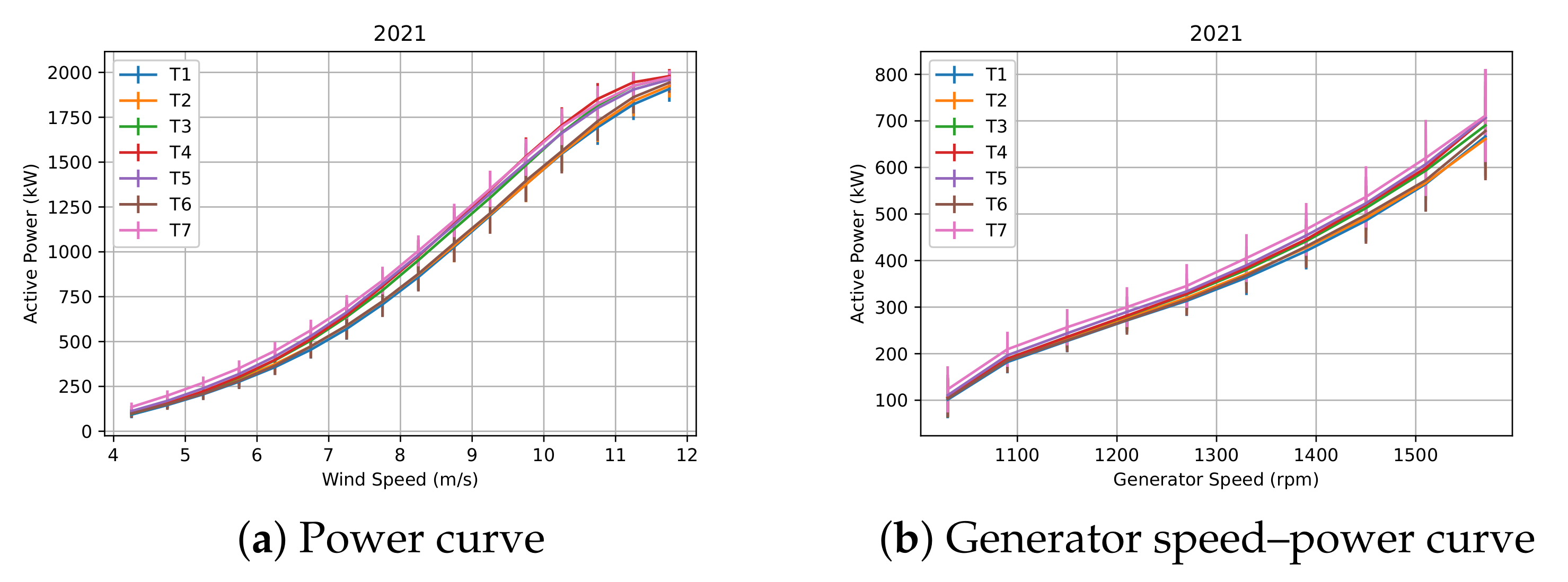
In Figure 7a, the average power curve for the wind farm is reported. From this figure, it arises that wind turbines T1, T2 and T6 are remarkably under-performing. A space comparison is pursued by training a model with the data of a reference wind turbine, which is selected as T5, and simulating for the other wind turbines. The results are reported in Table 8: it arises that T1, T2 and T6 have an under-performance below rated power in the order of 7.8%, 3.6%, 5.1% with respect to T5.
Given the above results, the generator speed–power curve is reported in Figure 7b. Similar to Section 4.1, the analysis of this operation curve that does not employ the wind speed corroborates the interpretation of the under-performance: wind turbines T1, T2 and T6 are those which extract less power for a given rotational speed.
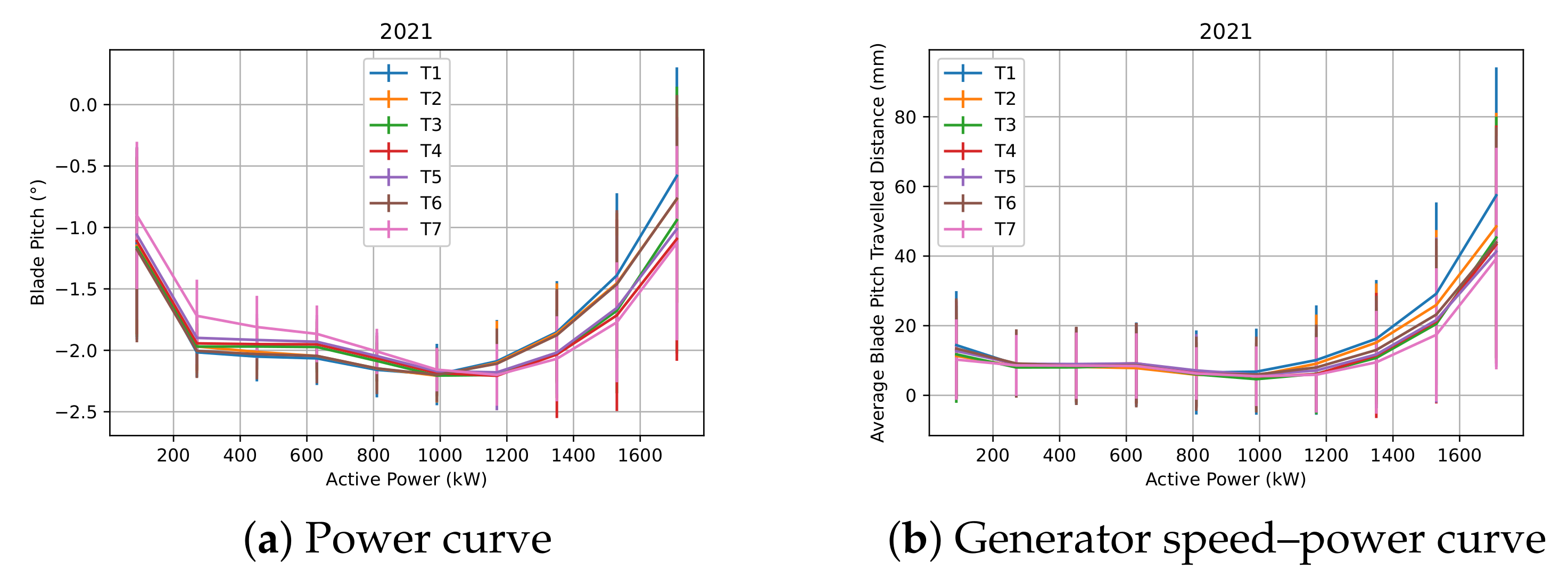
In Figure 8a, the active power–blade pitch curve is reported, from which it arises that wind turbines T1, T2 and T6 distinguish with respect to the rest of the wind farm, especially approaching rated power. In particular, the wind turbine that distinguishes more is the most under-performing one (T1). Figure 8a supports the hypothesis that the behavior of the under-performing wind turbines might also be related to the blade pitch control for this test case. For this reason, in Figure 8b, the behavior of the blade pitch piston traveled distance is reported as a function of the power and T1, T2 and T6 results being distinguishable with respect to the other wind turbines in the farm.
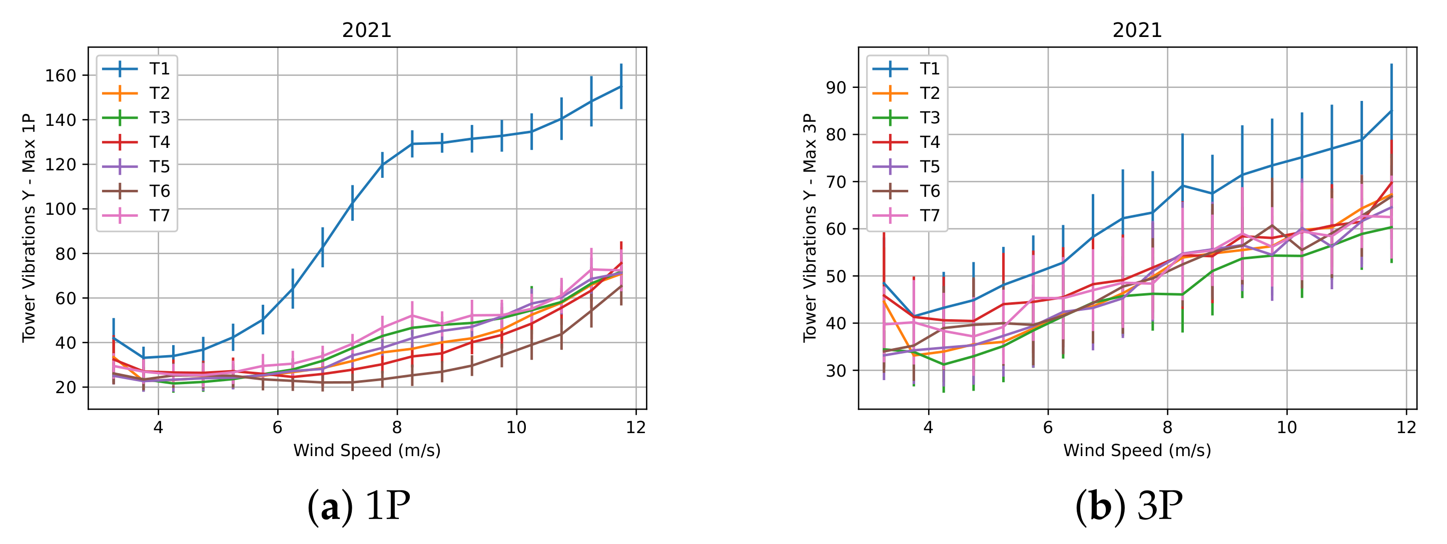
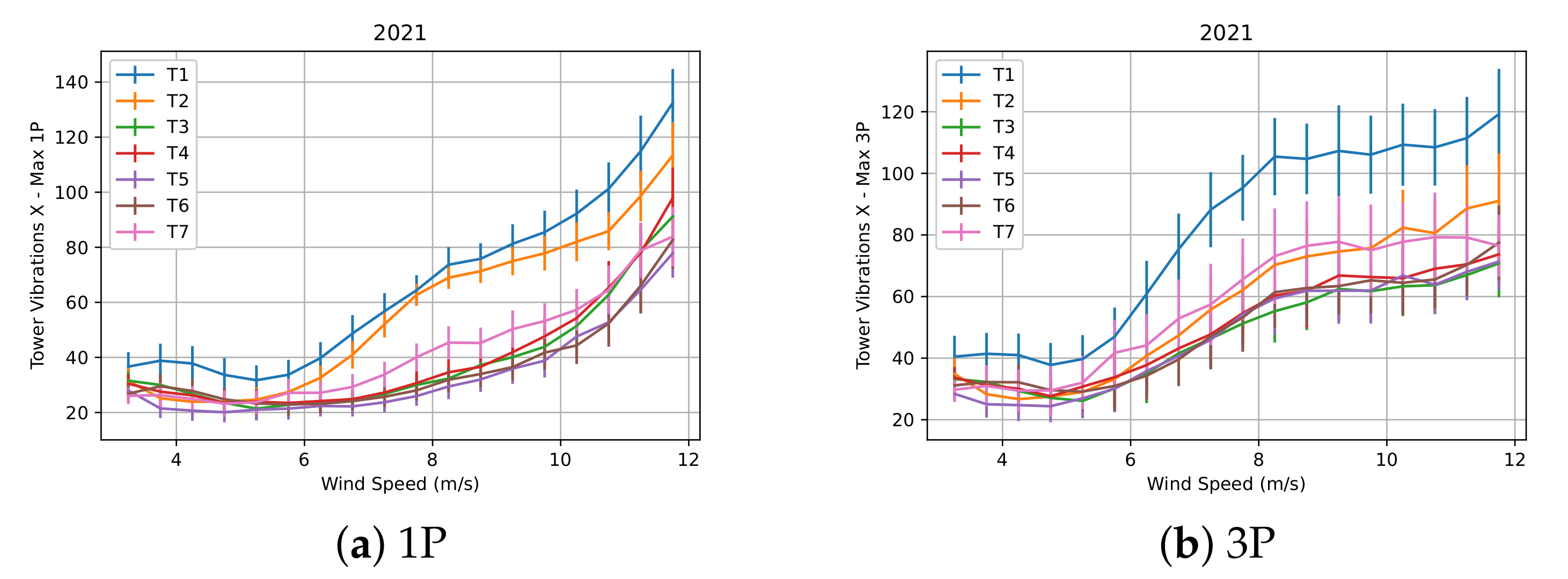
Finally, in Figure 9a,b and Figure 10,a,b, the behavior of the tower vibrations is characterized. The analyzed measurement channel is post-processed by the control system, which reports the amplitude of the longitudinal and transverse tower vibrations for the frequency component proportional to the rotor passing frequency (1P) and to the blade passing frequency (3P). Since wind turbines operate under non-stationary conditions, the 1P of course is not constant in time and the frequency components are extracted by the control system presumably through a Fast Fourier Transform. From Figure 9a and Figure 10b, it arises that T1 and T2 are evidently anomalous with respect to the rest of the wind farm, and this is corroborated by the regression analysis (Table 8), which indicates that, for example, wind turbine T1 has in average order of 50% more transverse 1P vibrations with respect to T5. The 1P and 3P frequencies are monitored because an anomalous 1P and 3P behavior might indicate a rotor unbalance, due to blade pitch and/or mass. Actually, if an unbalance is present, anomalies should be visible as the unbalanced blade passes (1P), as the two balanced blades pass (2P) and as each blade passes (3P). Therefore, Figure 9a and Figure 10b suggest that the under-performance of T1 and T2 might be related to a rotor unbalance, affecting the behavior of the blade pitch: indeed, a preliminary inspection at turbine T2 indicated that this is likely to be the case.
In Table 9, the correlation coefficients of interest are reported. Similarly with what happens for WF1, in general the correlation is only moderate, but all the quantities reported in Table 9 are highlighted by the Granger analysis to be in causal relation with the power with very high statistical significance.
The presence of a systematic error is compatible with the fact that T1, T2 and T6 have been under-performing since a remarkable number of years and no particular trends in time have been observed. By this point of view, WF2 characterizes as a test case with different peculiarities with respect to WF1, and it is interesting to discuss similar and different aspects. The wind turbines in WF1 appear to have the same working behavior, with a slight degradation in time with respect to it for some wind turbines, and for others not. Some wind turbines in WF2 appear to have an almost different working behavior with respect to the rest of the wind farm: this is corroborated by Figure 8a, where two substantially different active power–blade pitch curves are visible.
In Table 10, the standard deviation of the power above rated speed is reported, and it remarkably arises that the most under-performing wind turbines (T1, T2 and T6) display higher values, in particular T1 and secondarily T2, which also have the higher level of tower vibrations.
4.3. WF3
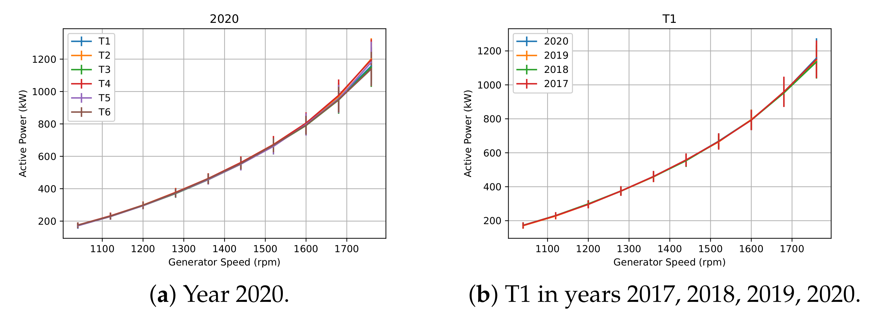
In Figure 11a, the average generator speed–power curve for WF3 is reported: it arises that the behavior of the wind turbines is extremely similar, and on average the same amount of power is extracted for the given rotational speed, differently with respect to what happens in WF1 and WF2. The quantitative estimates are reported in Table 11 based on a regression trained on the data of T1.
The behavior in time of the generator speed–power curve is reported for a sample wind turbine (T1) in Figure 11b. It arises that the behavior is extremely stable and a detailed time analysis based on the regression is pleonastic: from the figure, it arises that during the various years, T1 extracts on average the same amount of power for each given generator speed. The possibility of little time drifts is discussed in detail in [19] and is out of the scope of the present study. For the purposes of this work, the qualifying point is the comparison of Figure 11a against Figure 5a,b and Figure 7b.
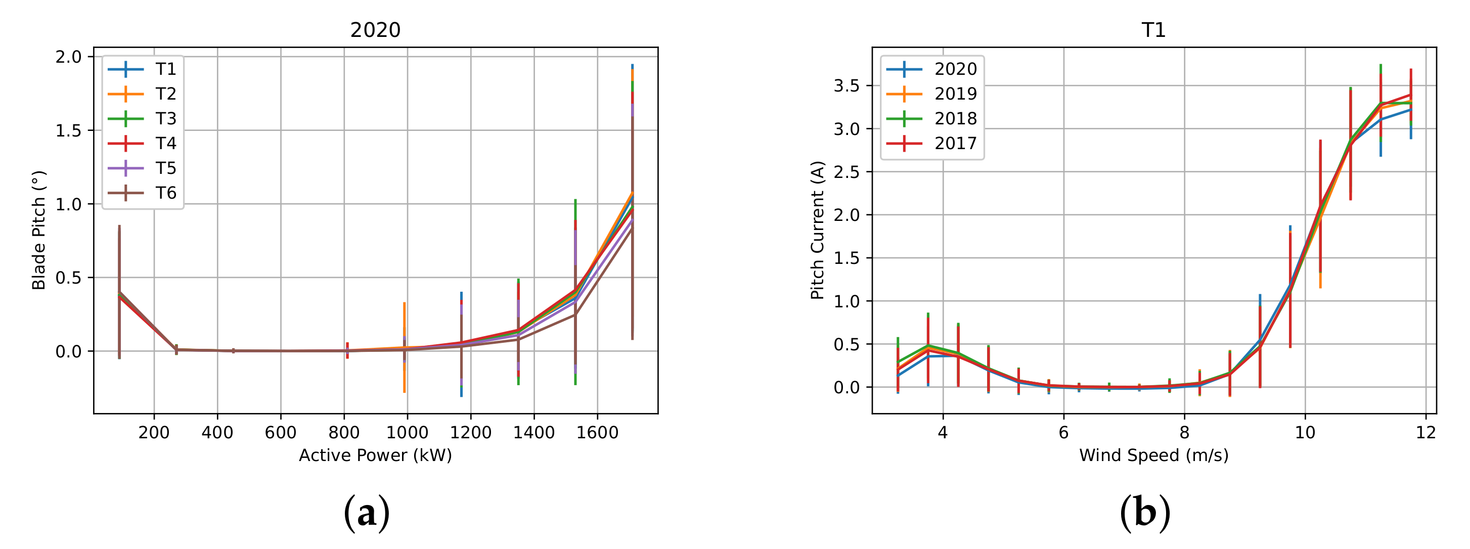
A similar line of reasoning can be applied to the active power–blade pitch curve, which is reported in Figure 12a. By comparing against Figure 8a, it arises that the curves for WF3 are much more similar for the various wind turbines. The curves for wind turbines T1–T5 are very compact and only wind turbine T6 displays a deviation with respect to the farm average; in any case, this variation is much more limited (maximum in the order of ) with respect to what happens in WF2 and is concentrated at rated rotational speed (which means power higher than that in Figure 11b, which instead refers to the regime where the blade pitch is employed to control the rotational speed).
In Figure 12b, the wind speed–blade pitch current is reported for a sample wind turbine for all the data sets at disposal from 2017 to 2020: a stable behavior arises.
It is interesting to notice that the correlation between blade pitch current and power is low (in the order of 0.15), but the Granger analysis still indicates a causal relation, although the significance is not as high as in the cases of WF1 and WF2. It is as if the electric blade pitch control requires less dynamic adjustment, resulting in lower correlation with the power, but guarantees a better regulation of the rotational speed, which therefore is very highly correlated with the power.
In Table 12, the standard deviation of the power above rated speed is reported and it arises that the values are quite homogeneous between the various wind turbines, differently with respect to what happens in particular in WF2.
4.4. Test Case Comparison
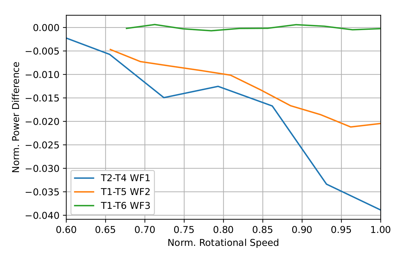
In Figure 13, a space comparison between the worst and the best performing wind turbines for each test case is reported. The x-axis is the rotational speed, normalized to the rated speed for each test case; the y-axis is the power difference between the best and worst performing turbines of the farm in unit of the rated power (which is the same for all the test case: 2 MW). From Figure 13, it clearly arises that for WF1 and WF2 there is much more difference than in WF3 in the amount of power that is extracted by the various wind turbines for a given rotational speed. As thoroughly discussed in the present study, the main difference between WF1 and WF2 on one side and WF3 on the other side is that the former two test cases are characterized by hydraulic blade pitch control and the latter by electrical pitch control. The results in Figure 13 therefore indicate that likely the electrical blade pitch is more capable, especially when the wind turbine ages, to control the machine and maintain it at an optimal working point, where the maximum amount of power is extracted for a given rotational speed.
5. Conclusions and Further Directions
The objective of the present study has been to develop SCADA data analysis methods for the interpretation of wind turbine performance. The work has been organized as a collaboration between academia (University of Perugia) and industry (Lucky Wind and ENGIE Italia utility companies), and this has provided the opportunity of discussing three real-world test cases: two of them (WF1 and WF2) have hydraulic pitch control and the other (WF3) has electric pitch control.
A first conclusion that can be drawn from the present analysis is that typically the information contained in the SCADA data sets is under-exploited. A qualifying contribution of the present study has been including measurement channels in the analysis which, to the best of the authors’ knowledge, have never been studied in detail in the literature. Actually, for an in deep comprehension of wind turbine performance, it is advisable to include in the analysis as many measurement channels as possible, which are related to the blade pitch control and to the behavior of the rotor. In particular, in this study, measurements of hydraulic pressure, piston traveled distance and tower vibrations have been analyzed for the wind turbines having hydraulic pitch control. For the wind turbines whose pitch control is electrical, it is advisable to monitor blade pitch currents. The selection of the above features has been motivated in this study through the analysis of correlation and statistical causal relation with the power: the achieved results indicate that the correlation is not a sufficient information for determining the features to employ for wind turbine monitoring. Actually, variables having low correlation with the power might be in causal relation with it and might give meaningful insight on the wind turbine behavior.
Based on the comparison of the three test cases, it has been observed that the wind turbines with hydraulic pitch control have a much wider variability in the amount of power extracted for a given rotational speed which, as discussed also in previous studies [16], is the most impacting manifestation of wind turbine under-performance. Through the analysis of the features selected expressly for this work, it has been possible to individuate that one test case is characterized by a decrease in time of blade pitch block manifold pressure and another test case is affected by anomalous tower vibrations and blade pitch behavior. The former can likely be interpreted as aging of the blade pitch actuators and the latter as a rotor unbalance (which has been confirmed by preliminary on-site inspection). For each critical test case, it has been observed that there is a reduced capability in maintaining the rated power above rated speed, with respect to the other wind turbines in the farm.
Therefore, the main result of this study is that it is plausible that the decline with age of wind turbine performance can often be ascribed to the behavior of the rotor, which is controlled through the blade pitch. The analysis of the two selected test cases indicates that this can occur in a variety of manners and with different severity, which should be analyzed case by case. Nevertheless, the individuation of the hydraulic pitch control as a sensible feature related to under-performance is an important indication for future studies.
The manifestations of wind turbine under-performance associated to blade pitch aging or, more in general, rotor issues which have been observed in this work are coherent with the findings in [30] and are:
- increased level of vibrations;
- decreased power stability above rated speed.
In this work, the observed under-performance has been elaborated in particular in the regime of variable rotational speed and the findings of [30] regarding the relation between blade pitch aging and currents behavior has been generalized to the case of hydraulic pitch with the analysis of pressures and piston traveled distance. It can be argued that the critical cases analyzed in this work might be affected also by overheating (as individuated in [30]), but the sub-components temperatures have not been at disposal for this study.
There is a vast amount of further directions of the present work, which at present the authors are pursuing. For example, advanced machine learning methods can be employed for putting in connection the measurement channels related to the rotor and the blade pitch to the observed power: in particular, clustering methods [33] and multivariate data integration methods [34] could be useful for interpreting the results more in depth.
The contributions of the present study can be related to the emerging trend of wind turbine lifetime assessment [3,35,36]. Detailed studies should be devoted to the lifetime analysis of the pros and cons of hydraulic and electric blade pitch control. It is likely that the former has a lower failure rate, but causes more under-performance and vice versa for the latter: a detailed balance of these aspects is definitely non-trivial and requires the individuation of appropriate indicators.
Author Contributions
Conceptualization, D.A., R.P., L.T. and A.L.; data curation, D.A. and A.L.; formal analysis, D.A.; investigation, D.A.; methodology, D.A. and A.L.; project administration, L.T.; software, D.A.; supervision, R.P. and L.T., validation, D.A., R.P., L.T. and A.L.; writing—original draft, D.A.; writing—review and editing, L.T. and A.L. All authors have read and agreed to the published version of the manuscript.
Funding
This research received no external funding.
Acknowledgments
The authors thank the company ENGIE Italia and Lucky Wind s.p.a. for the technical support and for providing the data sets employed for the study.
Conflicts of Interest
The authors declare no conflict of interest.
Abbreviations
The following abbreviations and symbols are used in this manuscript:
| IEC | International Electrotechnical Commission |
| SCADA | Supervisory Control And Data Acquisition |
| WF | Wind Farm |
| Wind Speed | v |
| Power | P |
| Generator speed | |
| Blade pitch | |
| Run time counter | |
| Pitch manifold pressure | |
| Blade pitch piston travelled distance | |
| Longitudinal tower vibrations 1P amplitude | |
| Longitudinal tower vibrations 3P amplitude | |
| Transverse tower vibrations 1P amplitude | |
| Transverse tower vibrations 3P amplitude | |
| Blade pitch current | I |
| Residual between measurement and model estimate | R |
| Average percentage change | |
| Pearson correlation coefficient | |
| Confidence level |
References
- Veers, P.; Dykes, K.; Lantz, E.; Barth, S.; Bottasso, C.L.; Carlson, O.; Clifton, A.; Green, J.; Green, P.; Holttinen, H.; et al. Grand challenges in the science of wind energy. Science 2019, 366, eaau2027. [Google Scholar] [CrossRef] [PubMed] [Green Version]
- Wood, D.H. Grand Challenges in Wind Energy Research. Front. Energy Res. 2020, 8, 337. [Google Scholar] [CrossRef]
- Mishnaevsky, L., Jr.; Thomsen, K. Costs of repair of wind turbine blades: Influence of technology aspects. Wind Energy 2020, 23, 2247–2255. [Google Scholar] [CrossRef]
- Carullo, A.; Ciocia, A.; Malgaroli, G.; Spertino, F. An Innovative Correction Method of Wind Speed for Efficiency Evaluation of Wind Turbines. ACTA IMEKO 2021, 10, 46–53. [Google Scholar] [CrossRef]
- Amato, A.; Heiba, B.; Spertino, F.; Malgaroli, G.; Ciocia, A.; Yahya, A.M.; Mahmoud, A.K. An Innovative Method to Evaluate the Real Performance of Wind Turbines With Respect to the Manufacturer Power Curve: Case Study from Mauritania. In Proceedings of the 2021 IEEE International Conference on Environment and Electrical Engineering and 2021 IEEE Industrial and Commercial Power Systems Europe (EEEIC/I&CPS Europe), Bari, Italy, 7–10 September 2021; pp. 1–5. [Google Scholar]
- Kurz, R.; Brun, K. Degradation of gas turbine performance in natural gas service. J. Nat. Gas Sci. Eng. 2009, 1, 95–102. [Google Scholar] [CrossRef]
- Carullo, A.; Castellana, A.; Vallan, A.; Ciocia, A.; Spertino, F. In-field monitoring of eight photovoltaic plants: Degradation rate over seven years of continuous operation. ACTA IMEKO 2018, 7, 75–81. [Google Scholar] [CrossRef]
- Staffell, I.; Green, R. How does wind farm performance decline with age? Renew. Energy 2014, 66, 775–786. [Google Scholar] [CrossRef] [Green Version]
- Olauson, J.; Edström, P.; Rydén, J. Wind turbine performance decline in Sweden. Wind Energy 2017, 20, 2049–2053. [Google Scholar] [CrossRef]
- Germer, S.; Kleidon, A. Have wind turbines in Germany generated electricity as would be expected from the prevailing wind conditions in 2000–2014? PLoS ONE 2019, 14, e0211028. [Google Scholar] [CrossRef]
- Hamilton, S.D.; Millstein, D.; Bolinger, M.; Wiser, R.; Jeong, S. How does wind project performance change with age in the United States? Joule 2020, 4, 1004–1020. [Google Scholar] [CrossRef]
- Benini, G.; Cattani, G. Measuring the long run technical efficiency of offshore wind farms. Appl. Energy 2022, 308, 118218. [Google Scholar] [CrossRef]
- Dai, J.; Yang, W.; Cao, J.; Liu, D.; Long, X. Ageing assessment of a wind turbine over time by interpreting wind farm SCADA data. Renew. Energy 2018, 116, 199–208. [Google Scholar] [CrossRef] [Green Version]
- Kim, H.G.; Kim, J.Y. Analysis of Wind Turbine Aging through Operation Data Calibrated by LiDAR Measurement. Energies 2021, 14, 2319. [Google Scholar] [CrossRef]
- Byrne, R.; Astolfi, D.; Castellani, F.; Hewitt, N.J. A Study of Wind Turbine Performance Decline with Age through Operation Data Analysis. Energies 2020, 13, 2086. [Google Scholar] [CrossRef] [Green Version]
- Astolfi, D.; Byrne, R.; Castellani, F. Analysis of Wind Turbine Aging through Operation Curves. Energies 2020, 13, 5623. [Google Scholar] [CrossRef]
- Astolfi, D.; Byrne, R.; Castellani, F. Estimation of the Performance Aging of the Vestas V52 Wind Turbine through Comparative Test Case Analysis. Energies 2021, 14, 915. [Google Scholar] [CrossRef]
- Astolfi, D.; Malgaroli, G.; Spertino, F.; Amato, A.; Lombardi, A.; Terzi, L. Long Term Wind Turbine Performance Analysis Through SCADA Data: A Case Study. In Proceedings of the 2021 IEEE 6th International Forum on Research and Technology for Society and Industry (RTSI), Naples, Italy, 6–9 September 2021; pp. 7–12. [Google Scholar]
- Astolfi, D.; Castellani, F.; Lombardi, A.; Terzi, L. Data-driven wind turbine aging models. Electr. Power Syst. Res. 2021, 201, 107495. [Google Scholar] [CrossRef]
- Lyons, J.T.; Göçmen, T. Applied machine learning techniques for performance analysis in large wind farms. Energies 2021, 14, 3756. [Google Scholar] [CrossRef]
- Ding, Y.; Kumar, N.; Prakash, A.; Kio, A.E.; Liu, X.; Liu, L.; Li, Q. A case study of space-time performance comparison of wind turbines on a wind farm. Renew. Energy 2021, 171, 735–746. [Google Scholar] [CrossRef]
- Pandit, R.K.; Infield, D. Comparative analysis of binning and Gaussian Process based blade pitch angle curve of a wind turbine for the purpose of condition monitoring. J. Phys. Conf. Ser. 2018, 1102, 012037. [Google Scholar] [CrossRef]
- Chen, W.; Wang, X.; Zhang, F.; Liu, H.; Lin, Y. Review of the application of hydraulic technology in wind turbine. Wind Energy 2020, 23, 1495–1522. [Google Scholar] [CrossRef]
- De Caro, F.; Vaccaro, A.; Villacci, D. Adaptive wind generation modeling by fuzzy clustering of experimental data. Electronics 2018, 7, 47. [Google Scholar] [CrossRef] [Green Version]
- IEC. Power Performance Measurements of Electricity Producing wind Turbines; Technical Report 61400–12; International Electrotechnical Commission: Geneva, Switzerland, 2005. [Google Scholar]
- Shokrzadeh, S.; Jozani, M.J.; Bibeau, E. Wind turbine power curve modeling using advanced parametric and nonparametric methods. IEEE Trans. Sustain. Energy 2014, 5, 1262–1269. [Google Scholar] [CrossRef]
- Wadhvani, R.; Shukla, S. Analysis of parametric and non-parametric regression techniques to model the wind turbine power curve. Wind Eng. 2019, 43, 225–232. [Google Scholar] [CrossRef]
- Charakopoulos, A.; Katsouli, G.; Karakasidis, T. Dynamics and causalities of atmospheric and oceanic data identified by complex networks and Granger causality analysis. Phys. A Stat. Mech. Its Appl. 2018, 495, 436–453. [Google Scholar] [CrossRef]
- Granger, C.W. Investigating causal relations by econometric models and cross-spectral methods. Econom. J. Econom. Soc. 1969, 37, 424–438. [Google Scholar] [CrossRef]
- Wei, L.; Qian, Z.; Zareipour, H.; Zhang, F. Comprehensive aging assessment of pitch systems combining SCADA and failure data. IET Renew. Power Gener. 2022, 16, 198–210. [Google Scholar] [CrossRef]
- Astolfi, D.; Pandit, R.; Celesti, L.; Vedovelli, M.; Lombardi, A.; Terzi, L. Data-Driven Assessment of Wind Turbine Performance Decline with Age and Interpretation Based on Comparative Test Case Analysis. Sensors 2022, 22, 3180. [Google Scholar] [CrossRef]
- Muljadi, E.; Butterfield, C.P. Pitch-controlled variable-speed wind turbine generation. IEEE Trans. Ind. Appl. 2001, 37, 240–246. [Google Scholar] [CrossRef] [Green Version]
- Bette, H.M.; Jungblut, E.; Guhr, T. Non-stationarity in correlation matrices for wind turbine SCADA-data and implications for failure detection. arXiv 2021, arXiv:2107.13256. [Google Scholar]
- Zaitouny, A.; Fragkou, A.D.; Stemler, T.; Walker, D.M.; Sun, Y.; Karakasidis, T.; Nathanail, E.; Small, M. Multiple sensors data integration for traffic incident detection using the quadrant scan. Sensors 2022, 22, 2933. [Google Scholar] [CrossRef] [PubMed]
- Alsaleh, A.; Sattler, M. Comprehensive life cycle assessment of large wind turbines in the US. Clean Technol. Environ. Policy 2019, 21, 887–903. [Google Scholar] [CrossRef]
- Amiri, A.K.; Kazacoks, R.; McMillan, D.; Feuchtwang, J.; Leithead, W. Farm-wide assessment of wind turbine lifetime extension using detailed tower model and actual operational history. J. Phys. Conf. Ser. 2019, 1222, 012034. [Google Scholar] [CrossRef]
Figure 1.
Sample yearly wind direction and intensity roses for the considered test cases.

Figure 2.
An example of scattered and binned generator speed–power curve for WF3.

Figure 3.
The average yearly power curve for the WF1 in the year 2021.

Figure 4.
The average yearly power curve for WF1: years 2019 and 2021 in the form of difference with respect to 2017.
Figure 4.
The average yearly power curve for WF1: years 2019 and 2021 in the form of difference with respect to 2017.

Figure 5.
The average yearly generator speed–power curve for WF1: years 2019 and 2021 in the form of difference with respect to the year 2017.
Figure 5.
The average yearly generator speed–power curve for WF1: years 2019 and 2021 in the form of difference with respect to the year 2017.

Figure 6.
The average yearly generator speed–average pitch manifold pressure curve for WF1.

Figure 7.
Average curves for WF2 in the year 2021.

Figure 8.
Average yearly blade pitch curves for WF2.

Figure 9.
Wind speed–maximum amplitude of transverse tower vibration curves for WF2: 2021.

Figure 10.
Wind speed–maximum amplitude of longitudinal tower vibration curves for WF2: 2021.

Figure 11.
Generator speed–power curves for WF3.

Figure 12.
Blade pitch curves for WF3. (a) Blade pitch–power curve: year 2020. (b) Wind speed—blade pitch current for T1 in years 2017, 2018, 2019, 2020.
Figure 12.
Blade pitch curves for WF3. (a) Blade pitch–power curve: year 2020. (b) Wind speed—blade pitch current for T1 in years 2017, 2018, 2019, 2020.

Figure 13.
Normalized power difference between the worst and best performing wind turbine for each test case: the latest data set at disposal has been employed.
Figure 13.
Normalized power difference between the worst and best performing wind turbine for each test case: the latest data set at disposal has been employed.


Table 1.
Features of the data set.
| Wind Farm | Pitch Control | Rotor Diameter (m.) | Peculiar Measurements | Data Sets |
|---|---|---|---|---|
| WF1 | Hydraulic | 100 | Pitch Manifold Pressure (bar) | 2017, 2019, 2021 |
| WF2 | Hydraulic | 90 | - Average Blade Pitch Piston Travelled Distance (mm) - Longitudinal Tower Vibrations 1P Amplitude - Longitudinal Tower Vibrations 3P Amplitude - Transverse Tower Vibrations 1P Amplitude - Transverse Tower Vibrations 3P Amplitude | 2021 |
| WF3 | Electric | 92 | Average Blade Pitch Current I (A) | 2017–2020 |
Table 2.
List of analyzed operation curves.
| Wind Farm | Curve | Range | ||
|---|---|---|---|---|
| All | Power Curve | v | P | [4, 12] m/s |
| WF1 | Generator Speed—Power | P | [900, 1500] rpm | |
| WF2 | Generator Speed—Power | P | [1000, 1600] rpm | |
| WF3 | Generator Speed—Power | P | [1000, 1800] rpm | |
| WF1 | Generator Speed—Average pitch pressure | [900, 1500] rpm | ||
| WF2 - WF3 | Active Power—Blade pitch | P | [0, 2000] kW | |
| WF2 | Active Power—Blade pitch piston distance | P | [0, 2000] kW | |
| WF2 | Wind Speed—Longitudinal tower vibration 1P | v | [4, 12] m/s | |
| WF2 | Wind Speed—Longitudinal tower vibration 3P | v | [4, 12] m/s | |
| WF2 | Wind Speed—Transverse tower vibration 1P | v | [4, 12] m/s | |
| WF2 | Wind Speed—Transverse tower vibration 3P | v | [4, 12] m/s | |
| WF3 | Wind Speed—Average blade pitch current | v | I | [4, 12] m/s |
Table 3.
Arrangement of the data sets for space and time comparisons.
| Type of Comparison | Reference Data | Target Data |
|---|---|---|
| Space | Reference wind turbine | All the fleet |
| Time | Reference data set for a target wind turbine | Posterior data sets |
Table 4.
Space performance comparison for WF1 in year 2021, with reference to T4: the estimates are computed according to Equation (3).
Table 4.
Space performance comparison for WF1 in year 2021, with reference to T4: the estimates are computed according to Equation (3).
| T1 | T2 | T3 |
|---|---|---|
| −5.8% | −8.7% | −2.1% |
Table 5.
Time performance comparison for T2 and T4 in WF1 for the years 2019 and 2021 with respect to 2017: the estimates are computed according to Equation (3).
Table 5.
Time performance comparison for T2 and T4 in WF1 for the years 2019 and 2021 with respect to 2017: the estimates are computed according to Equation (3).
| Wind Turbine | 2019 | 2021 |
|---|---|---|
| T2 | −7.2% | −9.7% |
| T4 | −3.9% | −2.2% |
Table 6.
Time performance comparison for T2 and T4 in WF1 for the years 2019 and 2021 with respect to 2017, for the generator speed–power and generator speed–average pitch pressure curves: the estimates are computed according to Equation (3).
Table 6.
Time performance comparison for T2 and T4 in WF1 for the years 2019 and 2021 with respect to 2017, for the generator speed–power and generator speed–average pitch pressure curves: the estimates are computed according to Equation (3).
| Wind Turbine | Quantity | 2019 | 2021 |
|---|---|---|---|
| T2 | P | −5.7% | −7.1% |
| T4 | P | −3.7% | −1.6% |
| T2 | −0.5% | −0.8% | |
| T4 | +0.3% | +0.1% |
Table 7.
Standard deviation of the power above rated speed for WF1 (kW).
| Wind Turbine | 2017 | 2019 | 2021 |
|---|---|---|---|
| T2 | 8.9 | 11.3 | 13.2 |
| T4 | 8.3 | 9.2 | 11.4 |
Table 8.
Space performance comparison for WF2 in year 2021, with reference to T5: the estimates are computed according to Equation (3).
Table 8.
Space performance comparison for WF2 in year 2021, with reference to T5: the estimates are computed according to Equation (3).
| Quantity | T1 | T2 | T3 | T4 | T6 | T7 |
|---|---|---|---|---|---|---|
| P | −7.8% | −3.6% | −2.0% | −0.5% | −5.1% | 2.2% |
| 51.8% | 11.9% | 0.3% | −4.9% | −13.1% | 3.8% | |
| 16.1% | −1.3% | −6.2% | 3.7% | 8.9% | 2.2% | |
| 43.1% | 27.2% | 4.5% | 8.7% | 6.2% | 11.0% | |
| 39.3% | 11.8% | −2.8% | 3.8% | 13.1% | 16.4% |
Table 9.
Correlation coefficient with the power P.
| Quantity | |
|---|---|
| 0.61 | |
| 0.84 | |
| 0.49 | |
| 0.80 | |
| 0.68 |
Table 10.
Standard deviation of the power above rated speed for WF2 (kW).
| T1 | T2 | T3 | T4 | T5 | T6 | T7 |
|---|---|---|---|---|---|---|
| 12.02 | 5.9 | 3.8 | 3.5 | 4.3 | 5.3 | 4.2 |
Table 11.
Space comparison for WF3 for the year 2020, for the generator speed–power curve, with T1 as reference: the estimates are computed according to Equation (3).
Table 11.
Space comparison for WF3 for the year 2020, for the generator speed–power curve, with T1 as reference: the estimates are computed according to Equation (3).
| T2 | T3 | T4 | T5 | T6 |
|---|---|---|---|---|
| 0.8% | −0.5% | 0.7% | −0.7% | −0.1% |
Table 12.
Standard deviation of the power above rated speed for WF3 (kW).
| T1 | T2 | T3 | T4 | T5 | T6 |
|---|---|---|---|---|---|
| 8.5 | 8.8 | 9.1 | 7.5 | 7.5 | 7.9 |
Publisher’s Note: MDPI stays neutral with regard to jurisdictional claims in published maps and institutional affiliations. |
© 2022 by the authors. Licensee MDPI, Basel, Switzerland. This article is an open access article distributed under the terms and conditions of the Creative Commons Attribution (CC BY) license (https://creativecommons.org/licenses/by/4.0/).
Share and Cite
MDPI and ACS Style
Astolfi, D.; Pandit, R.; Terzi, L.; Lombardi, A. Discussion of Wind Turbine Performance Based on SCADA Data and Multiple Test Case Analysis. Energies 2022, 15, 5343. https://doi.org/10.3390/en15155343
AMA Style
Astolfi D, Pandit R, Terzi L, Lombardi A. Discussion of Wind Turbine Performance Based on SCADA Data and Multiple Test Case Analysis. Energies. 2022; 15(15):5343. https://doi.org/10.3390/en15155343
Chicago/Turabian StyleAstolfi, Davide, Ravi Pandit, Ludovico Terzi, and Andrea Lombardi. 2022. "Discussion of Wind Turbine Performance Based on SCADA Data and Multiple Test Case Analysis" Energies 15, no. 15: 5343. https://doi.org/10.3390/en15155343
Note that from the first issue of 2016, this journal uses article numbers instead of page numbers. See further details here.