Systematic Review on Impact of Different Irradiance Forecasting Techniques for Solar Energy Prediction

Abstract

As non-renewable energy sources are in the verge of exhaustion, the entire world turns towards renewable sources to fill its energy demand. In the near future, solar energy will be a major contributor of renewable energy, but the integration of unreliable solar energy sources directly into the grid makes the existing system complex. To reduce the complexity, a microgrid system is a better solution. Solar energy forecasting models improve the reliability of the solar plant in microgrid operations. Uncertainty in solar energy prediction is the challenge in generating reliable energy. Employing, understanding, training, and evaluating several forecasting models with available meteorological data will ensure the selection of an appropriate forecast model for any particular location. New strategies and approaches emerge day by day to increase the model accuracy, with an ultimate objective of minimizing uncertainty in forecasting. Conventional methods include a lot of differential mathematical calculations. Large data availability at solar stations make use of various Artificial Intelligence (AI) techniques for computing, forecasting, and predicting solar radiation energy. The recent evolution of ensemble and hybrid models predicts solar radiation accurately compared to all the models. This paper reviews various models in solar irradiance and power estimation which are tabulated by classification types mentioned.

1. Introduction

The abundant availability of different forms of renewable energy and the latest renewable energy-harvesting technological improvement look attractive for world energy producers [1]. In addition, due to mass production of renewable energy components, the per unit cost of renewable energy products has come down drastically. Government policies encourage energy producers to generate more energy from renewable energy. India has committed to the ‘Mission 500 GW plan that sets a target of expanding the scope of renewable energy capacity to 500 GW by 2030. Solar and wind provide major contributions of renewable energy out of which solar PV-based power generation is a widely preferred option due to easy transportation, maintenance, and availability, etc. [2]. Photovoltaic and renewable energy capacity additions in GWs are illustrated in Figure 1 and Figure 2, respectively.

In solar power generation, the other option of solar thermal systems has been getting attraction in recent years. A concentrated solar power system can have high power generation capacity and can store thermal energy easily [3]. The high initial cost limitation, i.e., the requirement of both solar and steam plants that limits the advantage of thermal energy storage technologies in CSP even though they have better performance in integrating with the grid, is a drawback for both types of systems. The photovoltaic system reduces cost in the current market as it favors photovoltaic installations.

Many PV investors and producers are participating directly in electricity markets, minimizing financial penalties for any imbalance between generation, production, and supply. These problems are quite common in renewable energy source integration into the grid, i.e., because of stand-alone and grid-connected systems [4]. At any particular time, the generated electricity should be balanced with load usage. The plant should be designed such that it should handle changes, disturbances in the load, and faults in the power system grid, and it should provide continuous electricity to the customers. An accurate solar radiation forecasting method is required to control the losses and voltage sags and improve the reliable transmission of electricity. Accurate forecasts of the power output of PV plants maintain the economical and secure operation of the power system. They are also used for estimating the storage reserves, trading, scheduling power management, and reducing electricity production costs.

The persistence model forecasts solar energy based on previous solar radiation. The physical approach deals with data from weather stations and satellites that include numerical weather prediction (NWP), or satellite images to obtain solar forecasts. Time series-based forecasting models are statistical models that have been used for solar energy estimation [5]. There are two basic time series models: the Autoregressive (AR) model and the Moving Average (MA) model. The combination of these two yields several models such as Autoregressive Moving Average (ARMA); the Autoregressive Integrated Moving Average (ARIMA) model; the Autoregressive Fractionally Integrated Moving Average (ARFIMA) model, i.e., a generalization of ARMA and ARIMA models; the the Seasonal Autoregressive Integrated Moving Average (SARIMA) model, a variation of ARIMA used for seasonal time series forecasting; Vector Auto-Regressive (VAR); Vector Auto-Regressive with exogenous inputs (VARX); Autoregressive Moving Average with exogenous inputs (ARMAX); and the coupled autoregressive and dynamical system (CARDS). The models that do not include a lot of mathematical calculations and take less time to predict the forecasted output are Artificial Intelligence (AI) models, sometimes named soft computing techniques. They include different methods such as machine learning (ML) algorithms, deep learning (DL) models, genetic algorithms (GA), fuzzy logic (FL), probabilistic models, Markov chains (MC), etc., to develop solar energy forecasters. These AI models are further divided into machine learning models, deep learning models, probabilistic models, and special artificial intelligence models in this paper.

The artificial neural network is a powerful forecasting tool for nonlinear analysis of data, and this model uses data as inputs to obtain the corresponding solar energy forecasted output. Machine learning algorithms require less data compared to deep learning and less time to compute. The accuracy of ANN drops with larger time horizons. The persistence models, time series-based models, and artificial intelligence models use statistical calculations and are taken under a common classification as statistical models. Statistical approaches use the stored data to train a model, compare the predicted values with the actual values, and predict the output through minimization of error. The solar direct normal irradiance, the diffuse irradiance, and the ground reflected irradiance sum up the total incoming solar irradiance. The individual percentage of these irradiances depends on factors such as climate, location, and other atmospheric conditions [6].

The main objective of this paper is to review the impact of different irradiance forecasting techniques for solar energy prediction. In this article, the survey is carried in the following aspects:

• This review work intends to give a clear and detailed understanding of different forecasting models used for solar radiation prediction and forecasting.
• It drafts a systematic understanding of the selection and application scopes of the various forecasting models. The forecasting models are classified into eight categories.
• The tabular literature summaries were made, which will provide a synopsis of the overall features of most of the significant research work developed in solar forecasting models. It also elaborates on details of various feature reduction techniques.
• The physical models, time series models, machine learning models, deep learning models, special artificial intelligence models, probabilistic models and hybrid and ensemble models, including the basic reference model, i.e., the persistence model, are the eight models explored in our discussion.

2. Classification of Forecasting Methods

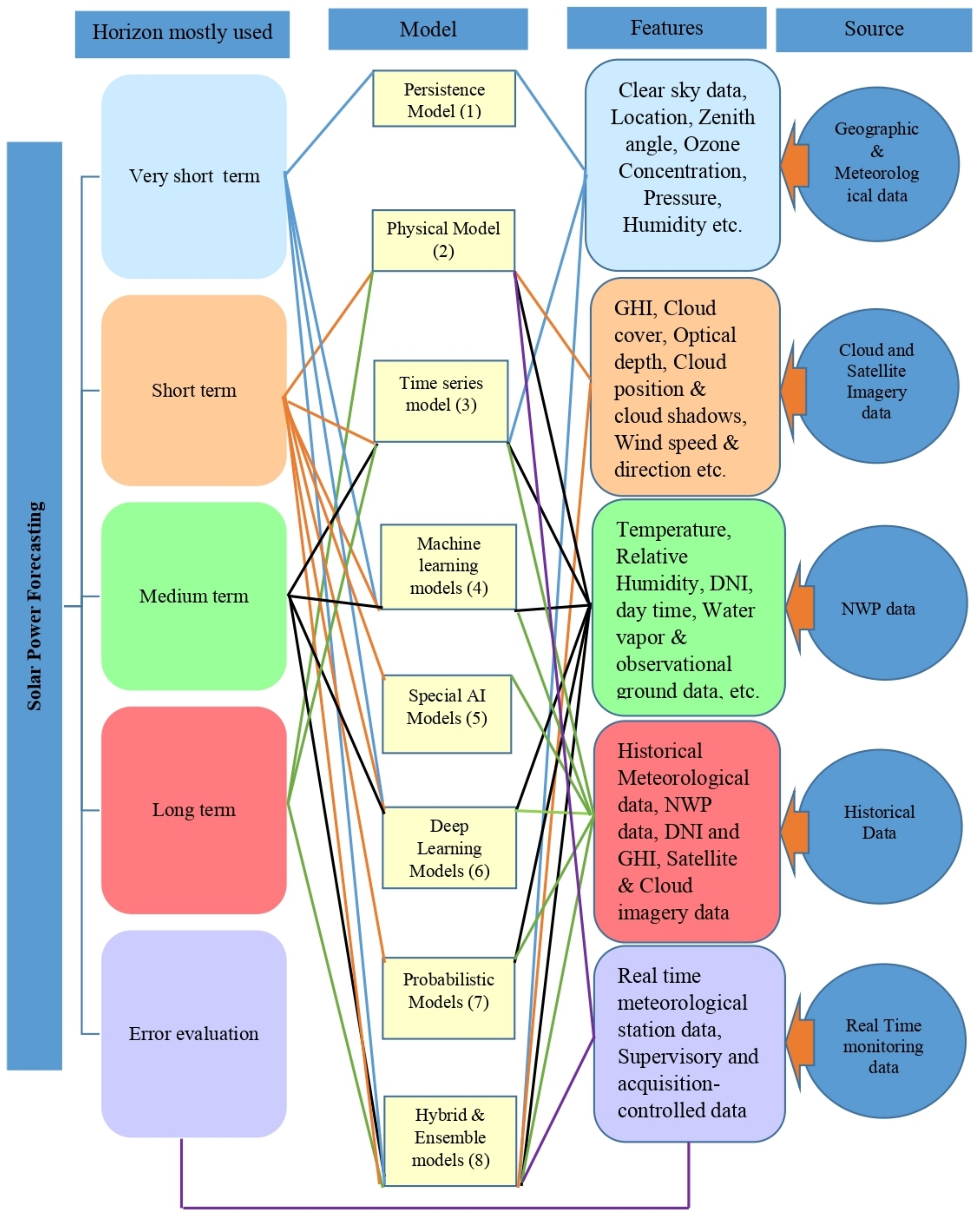
There are no constant classification criteria for solar forecasting. Researchers group PV power forecasting methods through different perspectives such as forecast scale, historical data, time horizon, location, and some other weather data. Based on the application, i.e., different aspects of grid operation, the major forecast classification is based on the time horizon. Depending on the spatial area, forecasting can be further labeled into local forecasts and regional forecasts. Considering the balance between supply and demand, regional forecasts are more preferred for plant and grid control operations.

2.1. Time Horizon

The time horizons are defined as the time interval to the times solar energy has to be forecast from the present time. The clustering of time horizons [7] decides the applications where solar energy has to be used. The time duration decides the model that best suits the accurate PV power forecast. Before the selection of the model, a proper time horizon should be selected to obtain a forecast with acceptable accuracy. Solar forecasting is classified based on time horizon as immediate forecasting in the period of a few seconds to 1 h ahead. Short-term power forecasting are the time intervals carried out from 1 h to 48 h ahead. It helps in continuous monitoring of solar plants, variable load control in solar energy markets, and in achieving unit commitment. Medium-term power forecasting ranges the time interval of 2 days to 1 week ahead and is preferred for maintenance and scheduling of PV power plants and its operations [8]. Long-term power forecasting takes the time interval from 1 week to 1 or more years and is used to plan solar power plants.

2.2. Spatial Resolution

Spatial Resolution is the measurement of the smallest object in the ground area drawn for the sensor or sensor’s instantaneous field of view. It is the linear dimension of the earth represented by each pixel. Many aspects such as temperature, humidity, moisture, etc., influence the area to be selected. Depending on the spatial region, the model used to predict solar power is chosen. The estimation of solar energy can be performed either for a single site or for a region [9]. Stand-alone or isolated systems distribute the power from the source to that particular site. They never transfer power to the grid or take from it, whereas in grid-connected systems, the power produced during peak periods is stored in a battery, and the excess power is sent to the grid. In off-peak times, sufficient power from the grid is taken to the site to meet its load

2.3. Forecast Theme

Theme of the forecast is important, whether the researchers are predicting solar irradiance or PV plant power directly [9]. Predicting solar PV power directly predicts the PV power output, and the former model estimates the output indirectly based on a plant’s performance.

2.4. Weather Factors

Before forecasting solar power, a researcher should look into two major points [10].

• Effect of primary weather elements determined from various PV analytical models and their contributions to the solar power forecast.
• Forecast of solar power ramping events caused by unexpected weather changes.

The classification survey of solar irradiance and power forecasting models is listed in

Table 1. Classification survey of solar irradiance and power forecasting models.

Reference	Title of the Paper	Year	Summary
S. Sreekumar et al. [11]	Solar power prediction models: classification based on time horizon, input, output and application	2018	Presents the classification of solar power forecast models majorly by type of inputs
Priya Gupta et al. [12]	PV power forecasting based on data-driven models: a review	2021	Presents the classification of solar power forecast models based on theme i.e., direct forecasting and indirect forecasting
J. Antonanzas et al. [13]	Review of photovoltaic power forecasting	2016	Presents the classification of solar power forecast models based on spatial region with single and regional solar power forecasts.
Muhammad Naveed Akhter et al. [7]	Review on forecasting of photovoltaic power generation based on machine learning and meta-heuristic techniques.	2019	Presents the classification of solar power forecast models based on time horizon of forecast.

.

3. Survey on Solar Irradiance and Power Forecasting Models

3.1. Survey on Persistence Models

Rui Huang et al. [14] used a system advisor model (SAM) to analyze previously generated solar data from solar anywhere. They performed their entire work in simulations in the system identification toolbox, Matlab platform. The authors concluded that the persistence model accurately predicts for very short-term solar power forecasting.

Prado-Rujas [15] et al. carried out an analysis between simple persistence and smart persistence models to predict solar irradiance. They verified these methods for 1, 11, 31, and 61 min. The simple persistence dominates for 1 and 11 min, whereas for 31 and 61 min, smart persistence works the best.

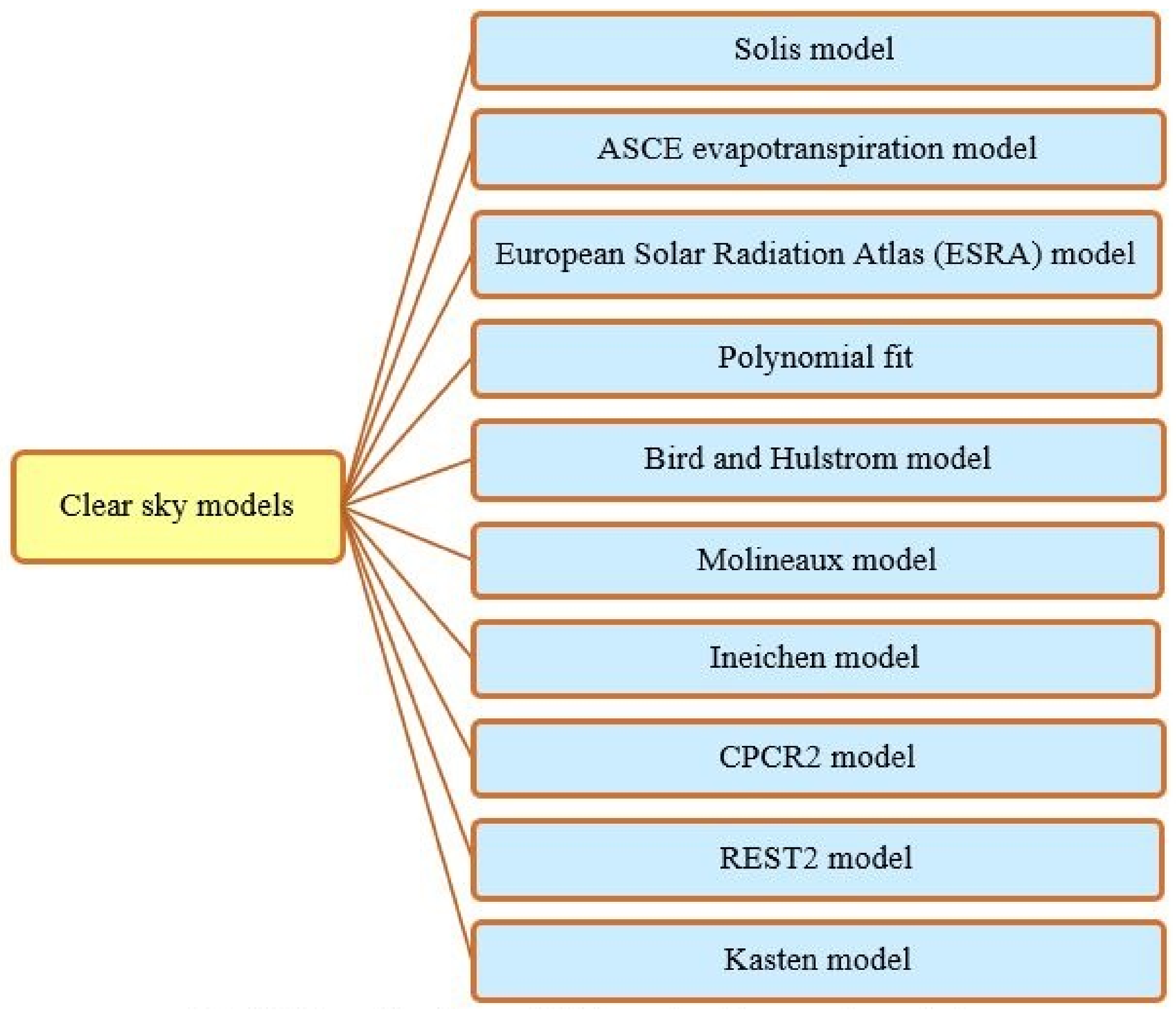
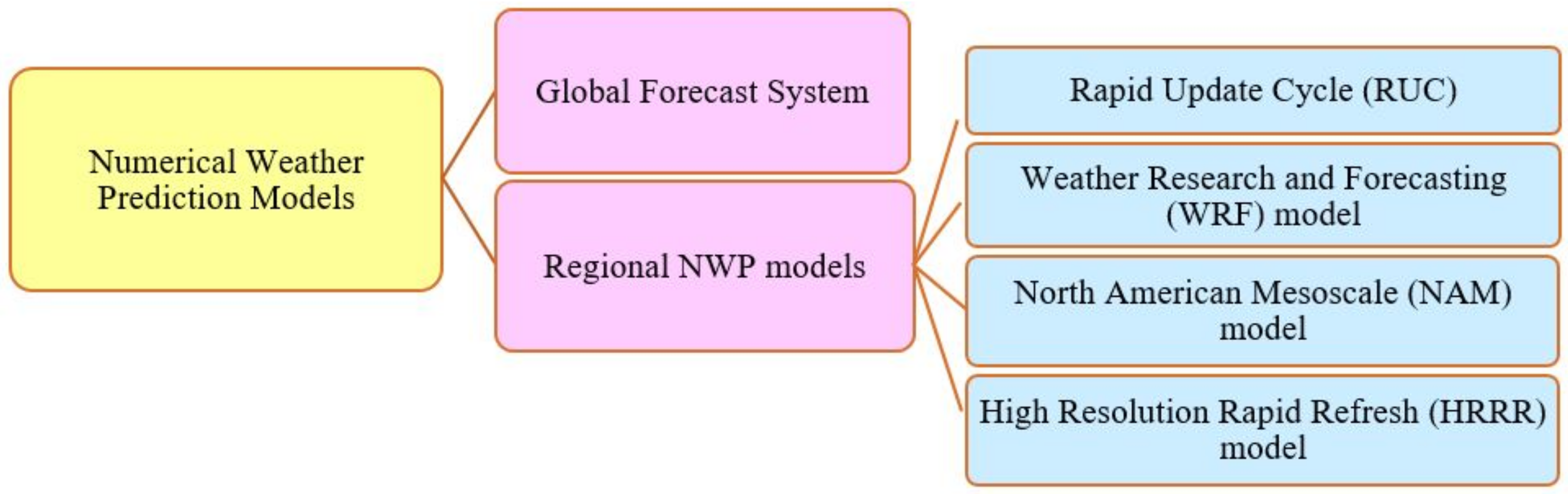
3.2. Survey on Physical Models

M.J. Mayer et al. [16] compared different physical models based on NWP data such as 9 separation, 10 transposition, 3 reflection, 5 cell temperature, 4 PV performance, 2 shading, and 3 inverter models on 16 PV plants to predict solar irradiance for intraday and day-ahead time horizons. The PHYSICAL reflection calculation, EVANS PV, beam shading calculation, and CONSTANT inverter efficiency models perform well with the best RMSE and MAE values.

Ozge et al. [17] compared various physical models such as 11 daily global solar radiation decomposition models and 7 different cell temperature models. The results prove that the CPRG model and the Skoplaki models perform better than other models respectively.

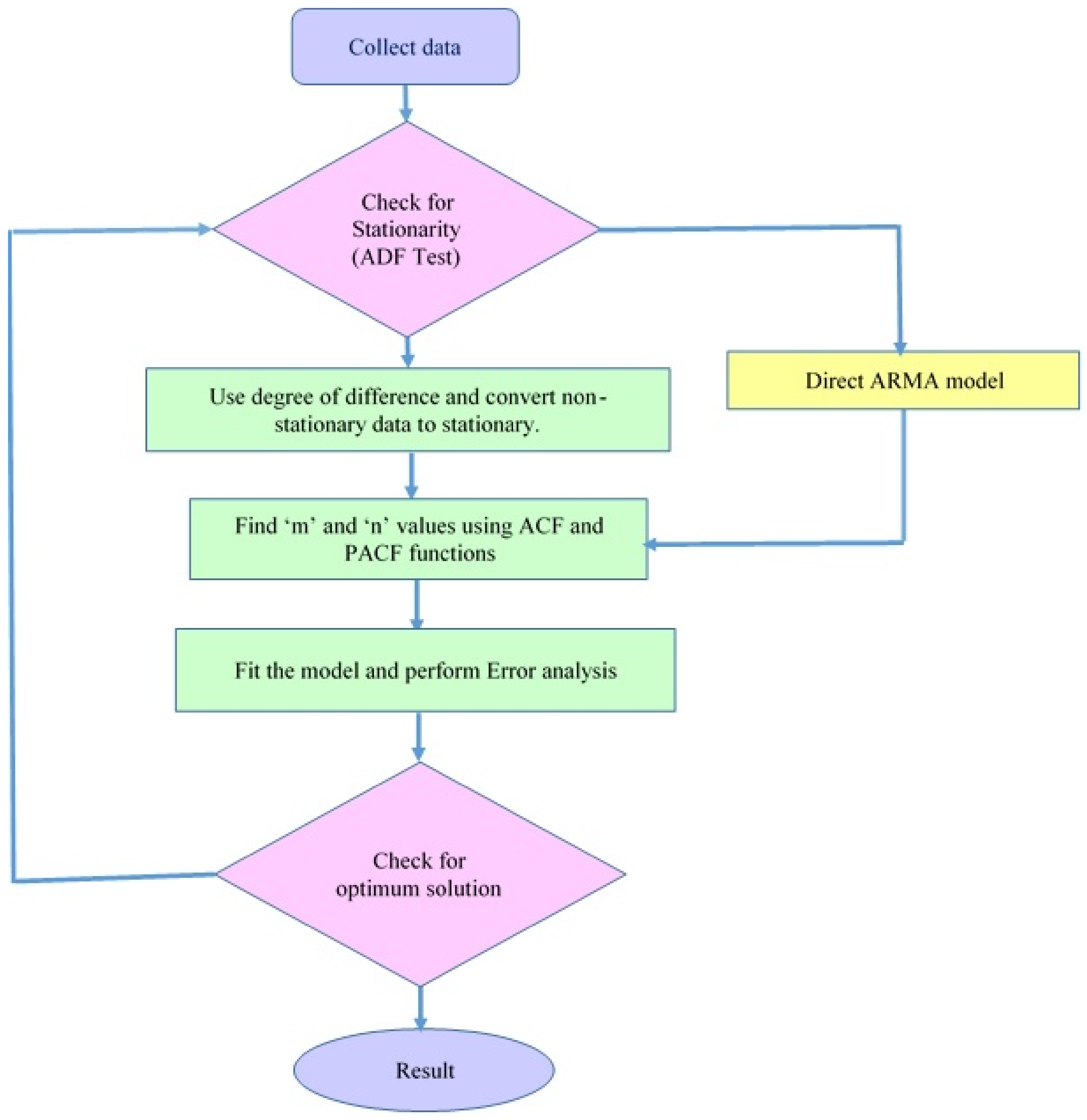
3.3. Survey on Time Series Models

Bismark Singh et al. [18] proposed an ARMA model with data taken from the Australian site. In 14 h of daily data, the Augmented Dickey–Fuller test (ADF) and the Ljung–Box test were used for each hour to test the stationarity and autocorrelation in the time series. The ARMA model was compared with the smart-persistence model to estimate solar radiance. The proposed ARMA model performs better than a smart-persistence model.

Rui Huang et al. [14] compared both the persistence and the ARMA model. For short- and medium-term solar power estimation in the microgrid operation, the authors dealt with reducing the error and suggested using the ARMA model rather than the persistence model.

Mbaye et al. [19] used the Akaike information to determine the p and q value of AR and MA models. The model uses the Box–Pierce test to analyze the error in the model, and the order (29, 0) fits the data and is reliable to the model performance with the acceptable white noise of 5%. The model was validated with metrics such as the RMSE = 0.629, the correlation coefficient = 0.963, the MAE = 0.528, and the MBE = 0.012.

Mohamad As’ad et al. [20] suggested ARIMA as the best model to find the solar power forecast up to seven days. One-year data from New South Wales, Australia, from June 2010 to May 2011 was considered for constructing a model. The results proved that the six months data is used to predict solar power for one day, and three months data is used for two or more than two days in a week.

Ilhami Colak et al. [21] proposed persistence, ARMA, and ARIMA models for one period, two periods, and three periods ahead for solar radiation forecast. The Log-Likelihood Function (LLF) tells whether the model fits the data or not. The accuracy of the ARMA (1, 2) and ARIMA (2, 2, 2) models was obtained by the metrics MAE and MAPE. ARIMA (2, 2, 2) gives the best results compared to the ARMA and persistence models.

Yanting Li et al. [22] evaluated five time series models such as ARMAX, ARIMA, single moving average, double exponential smoothing, and Holte Winter’s additive models for the one-day ahead forecasting of the mean daily output power of a 2.1 kW grid-connected PV system. The exogenous inputs such as daily average temperature, precipitation amount, insulation duration, and humidity were included in the ARMAX model for estimating solar power. These models were compared with the metrics RMSE, MAD, and MAPE. The results show the ARMAX model as the best with RMSE, MAD, and MAPE of 125.84, 98.61, and 82.69%, respectively, compared to the ARIMA (1, 1, 1) model. The authors also concluded the ARMAX model performs better than the neural network model for one-day head forecasting.

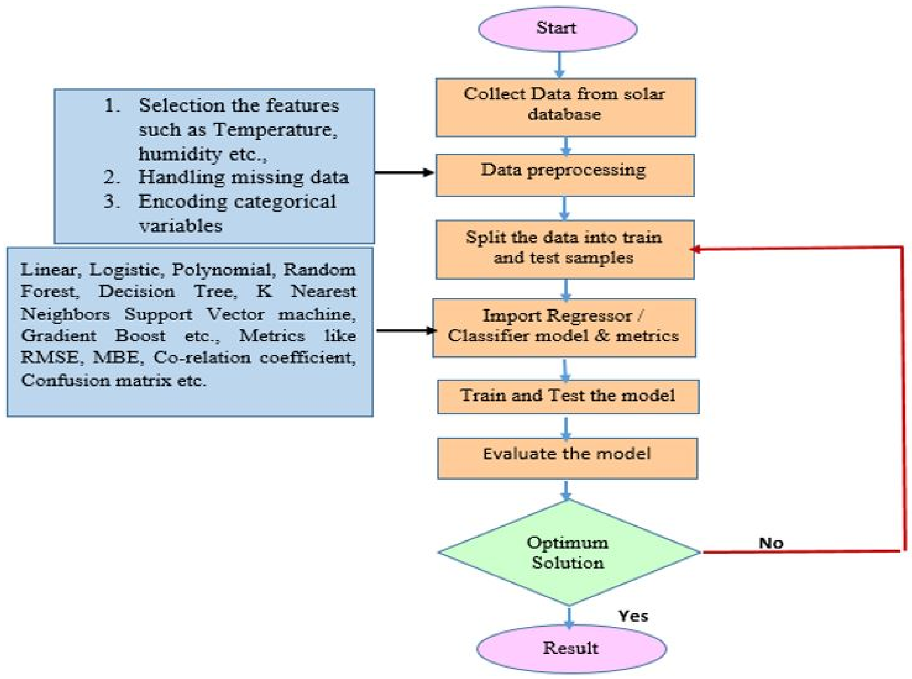
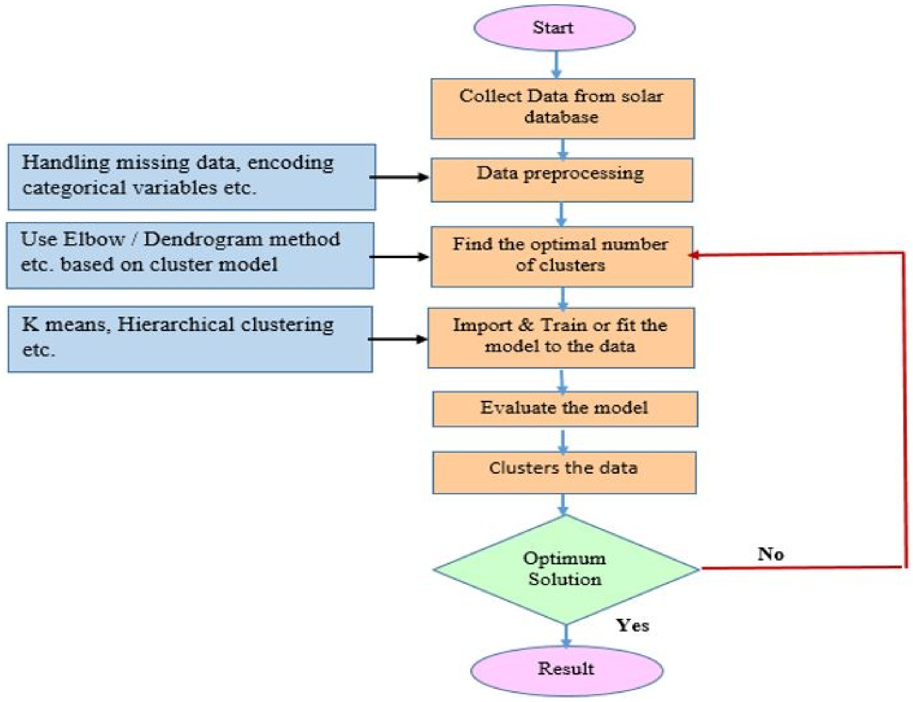
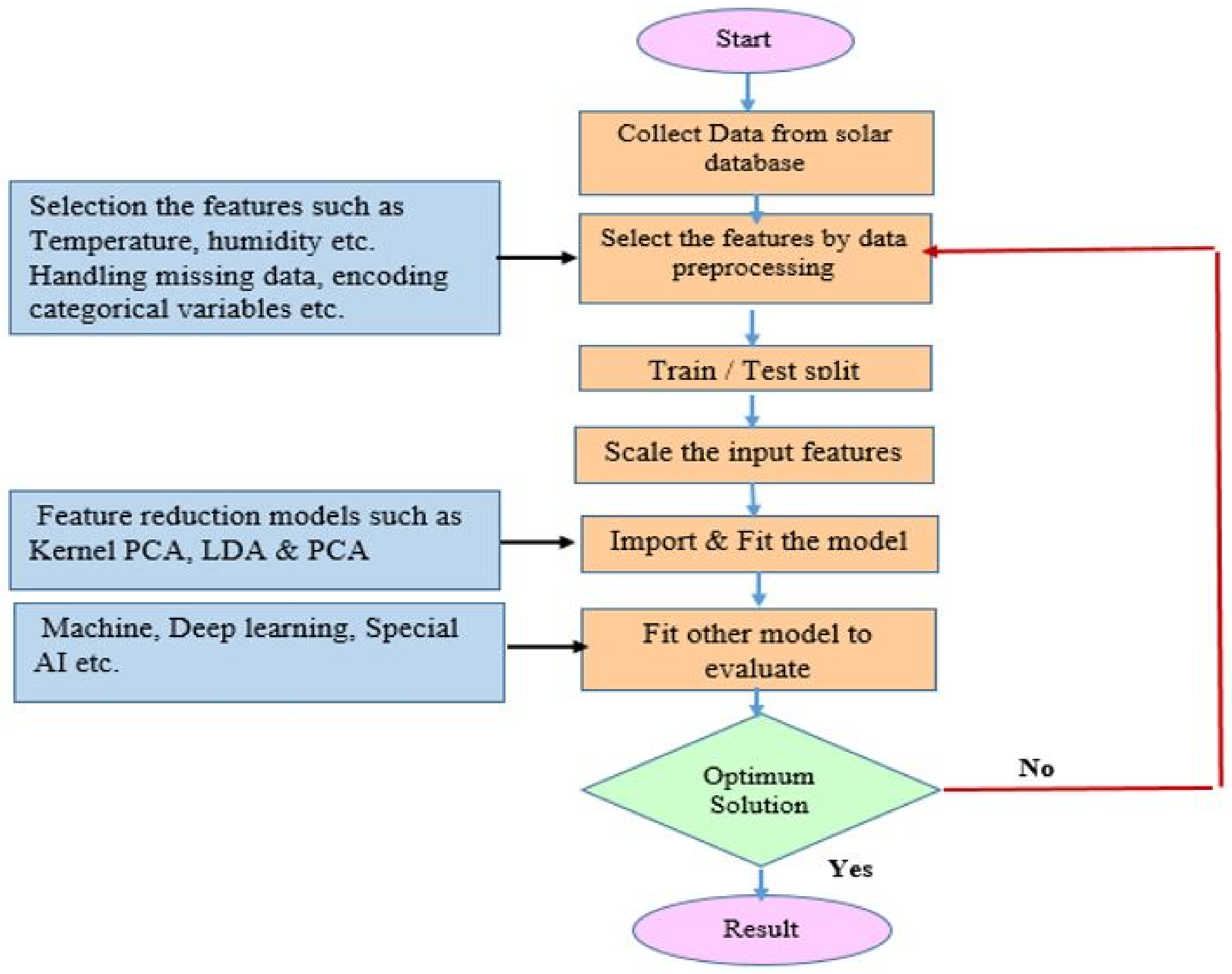
3.4. Survey on Machine Learning Models

Guo et al. [23] used the K-nearest neighbor (KNN) algorithm and two robust fusion algorithms. The authors used the KNN algorithm for the classification in the data and a mean square positioning error of less than 5 cm was achieved as result.

Leva et al. [24] used the ANN algorithm to forecast solar radiation 24 h ahead on three different days such as a sunny day, a partially cloudy day, and a cloudy day with one-year data taken from Italy.

Muhammad Waseem et al. [25] compared extra trees (ET) and random forest (RF) models with other popular machine learning algorithms for a PV system installed in Cardiff, UK. The authors proved these models perform better than support vector regression (SVR). The results show that the training and prediction time is less for the extra trees model compared to the random forest model.

Feng et al. [26] used a support vector machine model to recognize patterns in the first four hours of data to categorize a day in the forecasting stage for short-term solar power forecasting.

Hashemi et al. [27] proposed a paper to calculate snow loss on a PV farm in Ontario, Canada. The snow on the PV panel’s surface reduces solar energy generation. The authors compared five machine learning algorithms such as gradient boosted tree (GBT), random forest, regression tree (RT), recurrent artificial neural networks (RNN), and support vector regression. The results prove that the gradient boosted tree performed best.

C. Pan, J. Tan [28] proposed a paper on the prediction of day-ahead hourly solar power generation and divided the model into two parts: cluster analysis and an ensemble model (EM). To cluster the data, the authors compared spectral clustering (SC), hierarchical clustering (HC), and K-means clustering (KMC) models and the best method taken to cluster the data. Silhouette and the Calinski–Harabasz index also provided help to set the number of clusters to three. The authors concluded that spectral clustering and hierarchical clustering perform better than K-means clustering.

Jiaying Zhang, Yingfan Zhang [29] proposed a paper to predict solar power with data every 15 min from a China Electric Power Station. The density-based spatial clustering of applications with noise (DBSCAN) algorithm was used to cluster data, and thereby the bidirectional long short-term memory (Bi-LSTM) and conventional neural networks (CNN)-gate recurrent unit (GRU) are used on clustered data to forecast solar power, respectively. The authors concluded using the DBSCAN algorithm results in a prediction with a more accurate solution.

Souhaila Chahboun and Mohamed Maarouf [30] proposed a machine learning model to predict solar power. The authors removed unwanted features from the data and considered only six important features that vary 91% of the total variance. The machine learning methods applied to the output data of principal component analysis (PCA) and Bayesian regularized neural networks provided the best result.

Jiapeng Xiu et al. [31] combined principal components analysis and neural networks to forecast PV power. The authors analyzed past data, and through PCA, they transformed 30 inputs into 5 major inputs. Finally, they applied a neural network to estimate solar power to obtain an accurate prediction.

Shojaeighadikolaei et al. [32] proposed a study on the influence of day-ahead weather prediction on weather-aware distributed energy management in microgrids. Reinforcement learning (RL) is employed to improve the model’s accuracy. The outcomes show that the suggested distributed energy management algorithm can effectively deal with generation uncertainty.

3.5. Survey on Deep Learning Models

C.-J. Huang, P.-H. Kuo [33] presented a deep convolutional neural network model (CNN) for short-term PV power forecasting. The authors used a real-time solar power dataset from 2015. The model takes temperature, solar radiation, and PV system output power for the previous five days, and the result is an estimate of PV power for the next 24 h. The authors compare the proposed model with SVM, RF, decision tree (DT), multi-layer perceptron (MLP), and long short-term memory (LSTM) by the MAE and RMSE metrics. The results prove that the proposed model outperforms the other approaches.

Ahmad Alzahrani et al. [34] proposed a deep learning neural network model to forecast short-term solar irradiation. The authors took the data from a solar farm in Canada as input to the model. The training data input samples included four different weather conditions: few clouds, scattered clouds, overcast skies, and clear skies. This study compared the forward neural network (FNN), SVM, and LSTM models. The LSTM approach had the lowest RMSE and produced good outcomes. Among the other approaches, FNN had the worst performance. The performance of the support vector machine was superior to that of the FNN. The deep learning LSTM, on the other hand, outperformed the other approaches.

LIU et al. I [35] proposed a model using the backpropagation neural network (BPNN) to estimate day-ahead PV power in northwestern China. The proposed model included AI data as an extra input variable, leading to a significant reduction in average prediction error on cloudy days while maintaining similar prediction accuracy on sunny days.

WEN et al. [36] proposed a radial basis neural network (RBNN) model treated as a simplified MLP with only one hidden layer. The main differences between MLP and (radial basis function) RBF neural networks are that the linkages between the input and hidden layers in RBNN models are not weighted, and the activation functions on the nodes of the hidden layer are totally symmetrical. The Gaussian, multiquadric, inverse quadric, and polyharmonic spline functions are popular algorithms in RBNN networks. The parameters of RBNN are synaptic weights in the output layer, centers, and spread of the activation functions in the hidden layer. Although it is preferred to have the RBNN centers in each point in the input space, clustering chooses only a fraction of all possible points.

H.J. Lu et al. [37] used a radial basis function neural network with a decoupling method to estimate day-ahead PV power. The findings of the proposed paper compared the ARIMA, the backpropagation neural network (BPNN), and the radial basis function neural network (RBFNN). Finally, they concluded that the proposed model accurately predicts PV power compared to other models.

3.6. Survey on Special Artificial Intelligence Models

Ratshilengo et al. [38] used a genetic algorithm, a recurrent neural network, and K-nearest neighbor models to predict high-frequency solar irradiance from January 2020 to October 2020 data in South Africa. The genetic algorithm model predicted solar irradiance to the best mark with an optimum RMSE of 35.50 kW/m² and MAE of 26.74%.

3.7. Survey on Hybrid and Ensemble Models

Ospina et al. [39] developed a unique hybrid wavelet-based LSTM–deep neural network (DNN) forecasting model for predicting the PV power available in a PV system during a medium to short forecasting period. The results prove the suggested model forecasts the nonlinear response of solar power generation in a PV system and beat other examined models in prediction accuracy.

G Li et al. [40] used the Limberg solar power dataset to develop a hybrid deep learning model that uses artificial intelligence algorithms to predict solar power for short-term horizons. In this case, the model uses CNN to extract essential PV power and weather change features. By using past PV power data on the same date, LSTM generates a forecast for the subsequent time. The authors compared persistence, BPNN, and RBFNN with the hybrid algorithm. The simulation results show that the proposed method has low estimation error.

Seyed Mohammad et al. [41] proposed a hybrid solar irradiance forecasting model with a reinforcement approach. The authors used two different solar stations near Phoenix and Los Angeles in the United States to develop the model. The deep Q learning reinforcement learning technique decidespd the proper subsets of the combined deep optimized CNN models. The proposed deep RL-ensemble approach excelled at existing powerful standard algorithms in diverse time-step horizons.

Bendali et al. [42] proposed a novel hybrid method that uses a genetic algorithm to optimize the deep neural network for solar irradiance forecasting. The model uses 2016 to 2019 time series data of solar irradiance recorded from a Moroccan city. The performance of the developed models was evaluated rigorously for different seasons, including summer, autumn, winter, and spring. The GA-added deep learning models improved their performance significantly. The LSTM-GA and GRU-GA performed well compared to RNN-GA.

Tatiane et al. [43] used data of Algeciras, Spain and Petrolina, Brazil sites to develop an ensemble model of MLP, RBF, SOM, and CFBP. The 4-day data was chosen randomly from these sites to analyze the ensemble and individual models. The ensemble model outperforms the remaining models by the metrics RMSE of 24.086 W/m² and R of 0.996 in Spain and RMSE of 35.467 W/m² and $R^2$ of 0.988 in Brazil.

T. Ahmad et al. [44] proposed a K-nearest neighbor algorithm generalized linear regression (LR) model and an ensemble model for forecasting solar power. The mean absolute errors for the k-NN model in winter, spring, summer, and autumn are 1.62, 1.42, 1.19, and 1.29. This model predicts the best compared to the one-step-secant backpropagation neural network, decision tree, and BFGS quasi-Newton backpropagation neural network models.

Jing Bi et al. [45] proposed an integrated forecasting system based on a new combination of the Savitzky–Golay filter, wavelet decomposition (SGW), and stochastic configuration networks (SCNs). In addition, the research shows the SG filter outperforms the original, MA, and MM filter models with better prediction accuracy.

4. Statistical Metrics for Solar Power Forecasting

4.1. Pearson’s Correlation Coefficient ($R^2$)

Pearson’s correlation coefficient [46] gives the similarity of two sets, i.e., test and training set, through data visualization or some value-based percentage. It is indicated by ‘$\rho$’. The larger the ‘$\rho$’ is, the better the relation between the particular sets. In mathematics, it is represented as

$$\rho =\frac{cov(p,q)}{{\sigma }_p{\sigma }_q}$$

(1)

4.2. Root Mean Squared Error (RMSE)

RMSE compares two datasets with various scales. It gives error as output that went through the forecasting period verified with the train and test data split. It is given as [47]

$$RMSE=\sqrt{{\displaystyle \frac{1}{N}\sum _{k=0}^N{(p_k-q_k)}^2}}$$

(2)

where ‘$q_k$’ is the actual solar power generation at the kth time step; ‘$p_k$’ is the corresponding solar power generation estimated by a forecasting model; and N is the number of points estimated in the forecasting period.

RMSE is a function of three variables such as magnitude average error, number of error samples, and error distribution, and it gives some inappropriate values. Since it is taken root, it gives a small value, so large errors have some effect on the final result.

4.3. Normalized Root Mean Squared Error (NRMSE)

The normalized root mean square error (NRMSE) [9] compares the RMSE among the complete range of the observed variables. NRMSE is the division of the RMSE to the total variables observed. The mathematical expression is

$$NRMSE=\frac{RMSE}{P_{obs,max}-P_{obs,min}}$$

(3)

where ‘$P_{obs,max}$’ and ‘$P_{obs,min}$’ are the maximum and minimum variables. The difference between maximum and minimum gives a number of variables that are observed.

4.4. Maximum Absolute Error (MaxAE)

Absolute error is the deviation between the original and predicted values. The maximum absolute error gives the maximum deviation of it [46].

$$MaxAE=Max|p_k-q_k|$$

(4)

The MaxAE expresses the local difference of forecast errors. It is mainly used in short-term PV power forecasting.

4.5. Mean Absolute Error (MAE)

MAE gives the value of the average of absolute errors taken from two sets (predicted and original sets of data), i.e., by comparing every variable in a set and taking its deviation and averaging the deviations. This metric is mainly used to generate an error in linear regression analysis in machine learning algorithms [48].

$${\displaystyle MAE=\frac{1}{N}\sum _{k=1}^N|p_k-q_k|}$$

(5)

4.6. Mean Absolute Percentage Error (MAPE)

It is the division of MAE by the demand or capacity. It is also indicated as an average of absolute deviations of percentage errors [9].

$${\displaystyle MAPE=\frac{1}{N}\sum _{k=1}^N\frac{|p_k-q_k|}{Capacity}}$$

(6)

4.7. Mean Bias Error (MBE)

It is similar to mean absolute error. It gives the value of the average of many estimations taken from deviations for each value in the two sets [48].

$${\displaystyle MBE=\frac{1}{N}\sum _{k=1}^N|p_k-q_k|}$$

(7)

4.8. Kolmogorov–Smirnov Test Integral (KSI)

It helps in calculating the model’s capacity and propagating statistical observed distributions [46].

$$KSI={\int }_{x_{min}}^{x_{max}}{D}_{n}dx$$

(8)

4.9. Confusion Matrix (CM)

It is a table drawn between actual values and estimated values with positive and negative rates. In the table, the positive rate is denoted as one, and the negative rate with zero. The positive rates are given by true positives and true negatives, while the negative rates are false positives and false negatives. False-positive (FP) is a Type 1 error and false-negative (FN) is a Type 2 error. The model, should try to minimize Type 1 and Type 2 errors [49]. The confusion matrix in given in

Table 2. Confusion matrix.

		Actual Values
	T/F	1	0
Predicted values	1	TP	FP
	0	FN	TN

.

4.10. Accuracy

Accuracy is one of the measures of natural performance. It is defined as the ratio of the observations that are estimated correctly to overall observations. If the dataset is more balanced, then the more the accuracy metric performs well [49].

$$Accuracy=\frac{TP+TN}{TP+TN+FP+FN}$$

(9)

4.11. Precision

Precision is the ratio of positive observations that are assessed correctly of the total number of positive observations [49].

$$Precision=\frac{TP}{TP+FP}$$

(10)

4.12. Recall

It is defined as the number of positive predicted values present in the total actual positive values. It is also referred to as the true positive rate, and it is well known as sensitivity. For achieving good performance through recall in the model, the FN value should be low or reduced as much as possible [49].

$$Recall=\frac{TP}{TP+FN}$$

(11)

4.13. Forecast Score

It is defined as the ratio of prediction efficiency of the proposed model forecast to the prediction efficiency of the persistence forecast as given below [50].

4.13.1. $F_{\beta }$ Score

In some models, false positive and false negative are both important; then both precision and recall should be considered, or an $F_1$ score or $F_{\beta }$ is used.

If $\beta$ = 1, then it becomes $F_1$ score, and if $\beta$ = 0.5, then it is an F = 0.5 score. We can also select the $\beta$ value as 0.5, 1, 2….

$$F_{\beta }=\frac{(1+{\beta }^2)(Precision\times Recall)}{{\beta }^2\times Precision+Recall}$$

(12)

4.13.2. $F_1$ Score

$F_1$ score is the harmonic mean of precision and recall. It takes recall and precision both into account and finally gives the result.

$$F_{1}Score=\frac{2\times Precision\times Recall}{Precision+Recall}$$

(13)

If FP and FN are both important, then select $\beta$ = 1. Suppose the importance of FP is higher than FN; then select $\beta$ = 0.5, i.e., decrease the $\beta$ value below 1. In the same manner, increase $\beta$ value for the vice versa model.

5. Solar Irradiance and Power Forecasting Methodologies

5.1. Persistence Model

The persistence forecast model is used as the basic referral forecast method to compare and evaluate the performance of other advanced forecasting measures. The persistence method enables future data based on the past data with clear sky indices as a trivial model [51]. This model predicts the best with a clear sky or no clouds time interval and there obtains the change of error with solar irradiance. The accuracy of the persistence model is disturbed by the change of cloudiness. The summary of the physical models along with time-horizon-based results are shown in Table 3. The classification of the clear sky forecast models are shown in Figure 3.

Table 3. Summary of Basic models.

Reference	Year	Model	Location	Forecast Horizon	Data	Conclusion	Analysis
Yang et al. [52]	2012	Persistence	Orlando and Miami, USA	1 h ahead	Orlando 2005 October, and Miami 2004 December	RMSE value of 156.81 W/m2 in Miami 160.61 W/m2 in Orlando	Features can be further added from specific to tropical climates to improve forecasting.
Voyant et al. [53]	2012	Persistence	Mediterranean, France	1 h ahead	6 years data	Average nRMSE is 26.2%	Complex and costly to implement in real time Gid connected systems
Marquez et al. [54]	2013	Persistence	Davis and Merced, USA	30, 60, 90, and 120 min ahead	1 year, (1 January 2011 to 6 June 2011 and 23 November 2011 to 31 January 2012)	RMSE value of 61.24 to 107.47 W/m2	Low importance to the ANN architecture optimization analysis and to lag feature selection process.

Table 3. Summary of Basic models.

Reference	Year	Model	Location	Forecast Horizon	Data	Conclusion	Analysis
Yang et al. [52]	2012	Persistence	Orlando and Miami, USA	1 h ahead	Orlando 2005 October, and Miami 2004 December	RMSE value of 156.81 W/m2 in Miami 160.61 W/m2 in Orlando	Features can be further added from specific to tropical climates to improve forecasting.
Voyant et al. [53]	2012	Persistence	Mediterranean, France	1 h ahead	6 years data	Average nRMSE is 26.2%	Complex and costly to implement in real time Gid connected systems
Marquez et al. [54]	2013	Persistence	Davis and Merced, USA	30, 60, 90, and 120 min ahead	1 year, (1 January 2011 to 6 June 2011 and 23 November 2011 to 31 January 2012)	RMSE value of 61.24 to 107.47 W/m2	Low importance to the ANN architecture optimization analysis and to lag feature selection process.

Figure 3. Classification of clear sky forecast models [55].

Figure 3. Classification of clear sky forecast models [55].

5.1.1. Persistence Model 1

This model predicts the power y for all future times is the power y observed at the time of the forecast.

$$K_{t+1}=K_t+K_E$$

(14)

where $K_E$ is the error due to irradiance.

Persistence model 1 is a benchmark more suited to short-term forecasts.

5.1.2. Persistence Model 2

This model states the power forecast for a given time is the power observed the day before at the same time.

$$K_{t+1}=K_t+K_E-24\mathrm{h}$$

(15)

Persistence 2 model is a benchmark model for day-ahead forecasts.

The error increases with fast changes in solar irradiance. Estimation of the measured irradiance and the clear sky irradiance clusters the various persistence models. Since it forecasts through clear sky data, this model takes some time to display the energy that is predicted.

5.1.3. Smart Persistence Model

This model predicts based on previous values, and it includes some modifications to the persistence model. This model adds the calculated change of radiation based on clear sky irradiance. In this case, the data has to be standardized.

$$y(t+h)=y\left(t\right)+\left|y\left(t\right)\right|[\frac{I_{cs}(t+h)}{I_{cs}}-1]$$

(16)

5.2. Physical Model

Satellite imagery (SM) models are preferred to forecast the high spatial resolution cloudiness [56]. These models depend on locating the cloud’s position. The cloud cover and optical depth decide the satellite model performance. The classification of the satellite-based forecast models are shown in Figure 4. These models are used to forecast radiance up to 6 h ahead. The physical satellite models depend on atmospheric component interaction modeled by a radiative transfer model (RTM), and statistical satellite models depend on the regression between the pyrometer-based solar irradiance at ground level and simultaneous digital counts provided by satellite-based instruments [57].

Sky image (SI) models [58,59] are different from NWP and satellite models and are helpful in intra-hour solar forecasting. The physical models concerning sky images include cloud motion, cloud detection, and cloud classification. The solar radiance reaches the Earth’s surface through the atmosphere. Surface irradiance is highly sensitive to the clouds rather than air matter, vapor, and aerosols. The sky images give the cloud features such as brightness, size, shape, spectrum, and texture. The texture is a regional feature that describes the spatial distribution of each pixel in an image. From another perspective, the sky images alone perform the regional forecasts on different forecast horizons through a single camera. The sky imager takes the sky image. There are mainly two components in a sky imager camera and hemispherical mirror. A sunshade is required to shelter the camera from the direct solar radiance. It is on top of the hemispherical mirror with the support of the frame. Along with the sky imager, irradiance meters are in a PV power plant to picture the sky image and measure the irradiance simultaneously. Some parts of the sky image reduce the forecast’s accuracy by creating unwanted noise; so these parts should be separated and terminated. The forecast models based on the NWP physical system are clearly classified in Figure 5.

In numerical weather prediction models [60], numerical modeling of the atmosphere serves as the basis. The NWP model is a mixture of calculus and important physical relations of weather to vary the climatic conditions. In the NWP model, the physical laws predict the cloud coverage and solar radiation depending on the basis. It helps in forecasting the output up to 15 days in advance with more output time of prediction. The adequate extraction of features from the raw NWP data requires time in this data mining phase in addition to the choice of the statistical learning algorithm. The area and time concerns limit the detection of all features of cloud images in NWP models and cannot predict solar radiance for short time horizons. The metrical summary of various physical models based on satellite, sky image, and NWP data are shown in

Table 4. Summary of Physical models.

Reference	Year	Model	Location	Forecast horizon	Data	Conclusion	Analysis
Yeom et al. [61]	2019	Kawamura	Korea	1 h ahead	April 2011 to December 2017	RMSE of 91.79 W/m2	Misclassified results affect the forecast performance of solar radiation
Garniwa et al. [62]	2021	Beyer	Seoul, Korea	1 h ahead	2018 year data	RMSE of 118.95 W/m2	LSTM performs well than physical model
Garniwa et al. [62]	2021	Perez	Seoul, Korea	1 h ahead	2018 year data	RMSE of 89.67 W/m2	LSTM performs well than physical model
Pereira et al. [63]	2019	NWP	Evora and Sines, Portugal	1 h ahead	2015 year data	RMSE = 57.8–164.4 W/m2 based on sky condition	Increase in data can further improve forecast performance.
Mathiesen et al. [64]	2013	NWP	USA	1 h to 1 day ahead	Hourly GHI from the SURFRAD network	rMBE 17.8% and rMAE 25.4%	Based on the cloud parameters, resolution and ramp rate, the result can be further improved
Alfredo et al. [65]	2012	NWP	Spain	6 to 39 h ahead	362 days (2 June 2007 to 27 May 2008)	RMSE error of 11.79% of rated power output	Addition of new input parameters in the third module may increase further performance

.

5.3. Time-Series-Based Forecast Models

The auto-regressive moving average model is a well-known practical tool to estimate the future value of the stationary time series model. The auto regressive component predicts the future based on the previous data. The auto-correlation factor is the metric used in the AR method. The expression for the AR model (order m) is

$${\displaystyle X_t=c+\sum _{k=1}^m{\phi }_k{X}_{t-k}+{\epsilon }_t}$$

(17)

The moving average [66] component predicts the future based on the error or residual in the past data. The partial auto-correlation factor is the metric used in the MA method. The expression for the MA (order n) model is

$${\displaystyle X_t=\mu +\sum _{k=1}^n{\theta }_k{\epsilon }_{t-k}+{\epsilon }_t}$$

(18)

The auto-regressive moving average (ARMA) is the sum of auto-regressive and moving average components. It estimates the future value based on the past data and residual errors. The autoregressive moving average model can be expressed as

$${\displaystyle X_t=c+\sum _{k=1}^m{\phi }_k{X}_{t-k}+\sum _{k=1}^n{\theta }_k{\epsilon }_{t-k}+{\epsilon }_t}$$

(19)

The drawback of the ARMA model is it does not perform for non-stationary data. Below is an auto-regressive integrated moving average (ARIMA) model [51] to overcome that limitation. ARIMA combines three parts: an AR part, an MA part, and an integrated part (number of lagged differences (d) to reach stationary data from non-stationary data).

$$Y_t={(1-L)}^d{X}_t$$

(20)

$${\displaystyle (1-\sum _{k=1}^m{\phi }_k{L}^k){(1-L)}^d{X}_t=(1+\sum _{k=1}^n{\theta }_k{L}^k){\epsilon }_t}$$

(21)

The ARIMA model represents the form ARIMA (m, d, n). The drawback of the ARIMA model is it cannot take informative variables such as temperature, humidity, precipitation, etc. Including these variables leads to better accuracy. The auto-regressive moving average with exogenous inputs (ARMAX) model can take exogenous inputs into account to estimate solar output. A Hausman’s test determines the ‘p’ number of external inputs (order p) to the model. The ARMAX model combines m AR terms, n MA terms, and p exogenous inputs terms.

$${\displaystyle X_t=c+\sum _{k=1}^m{\phi }_k{X}_{t-k}+\sum _{k=1}^n{\theta }_k{\epsilon }_{t-k}+{\epsilon }_t+\sum _{k=1}^p{\delta }_k{d}_{t-k}}$$

(22)

where ‘$X_t$’ is the estimated solar irradiance at a time (t), ‘$X_{t-k}$’ is the past solar irradiance data up to ‘k’ times, ‘${\phi }_k$’is AR models coefficient, ‘${\theta }_k$’ is MA model coefficient, ‘m’ is AR model order, L indicates the lag operator, d is the number of non-seasonal differences, ‘n’ is MA model order, ‘${\epsilon }_t$’ is the white noise. Mathematically, ARIMA (m, d, n) can be converted to the ARMA (m, n) model when d = 0, the d order made the ARIMA a popular tool in time series forecasting to estimate solar power. Mathematically, ARMA (m, n) can be converted to the AR (m) model when n = 0 and to the MA (n) model when m = 0, ${\delta }_k$ is the parameter of the exogenous input. The computational summary of the time series models is shown in

Table 5. Summary of time series models.

Reference	Year	Model	Location	Forecast Horizon	Data	Conclusion	Analysis
Moreno-Munoz et al. [67]	2008	Auto Regressive	south Spain	5 min ahead	4 years data, (1994–1997)	Best Fit: 65%	The use of AI models enhance better prediction performance
Y. Li et al.  [68]	2014	Moving average	Coloane island, Macau	1 day ahead	1 January 2011 to 30 June 2012.	RMSE value of 196.22 W/m2	Analysis of cloud further enhance the performance
Bacher et al. [69]	2009	ARX	Small village in Denmark	Up to 36 h ahead	1 year data	RMSE improvement of 35% in ARX model over naïve predictor model.	Further forecast can be improved with other Time series and AI models Analysis of cloud further enhance the performance
Y. Li et al. [68]	2014	ARIMA	Coloane island of Macau	1 day ahead	1 January 2011 to 30 June 2012.	RMSE value of 171.73 W/m2	Analysis of cloud further enhance the performance
Yang et al. [52]	2012	ARIMA	Orlando and Miami, USA	1 h ahead	Orlando 2005 October, and Miami 2004 December	RMSE value of 29.73 W/m2 in Miami and 32.80 W/m2 in Orlando	Features can be further added from specific to tropical climates to improve forecasting.
Y. Li et al. [68]	2014	ARMAX	Coloane island of Macau	1 day ahead	1 January 2011 to 30 June 2012.	RMSE value of 125.84 W/m2	Analysis of cloud further enhance the performance
Ricardo et al. [70]	2015	VAR	Evora, Portugal	Six hours ahead	1 February 2011 and 6 March 2013	Improvement of 8% to 1.5% over AR model	The algorithms like GA, PCA for future selection can achieve better performance.
Ricardo et al. [70]	2015	VARX	Evora, Portugal	Six hours ahead	1 February 2011 and 6 March 2013	Improvement of 10% to 5.5% over AR model.	Addition of Weather station and NWP data enhance prediction accuracy.
Ines et al. [71]	2017	NARX	North of Barcelona	Any time	1 year 2010	RMSE value of 18.64%	The results should be compared with high solar radiation fluctuations.
Piazza et al. [72]	2016	NARX	Palemo, Silicy, Italy	1 h ahead	2002 to 2008	nRMSE value of 6.1%	The exogeneous variable has to be changed to new parameter from temperature to increase accuracy.
Voyant et al. [73]	2014	ARMA	Mediterranean, France	24 h ahead	10 years data	nRMSE ranges from 28.6 to 32.8%	The use of exogenous input increases the performance. Additionally, the deep and machine learning models can be applied to improve the result.

. The operational analysis of ARMA and ARIMA models with stationary dataset is described in Figure 6 by flowchart representation.

Artificial Intelligence (AI) is an interesting method to create machines that perform functions with intelligent minds. AI has the capability of human thinking, activities such as decision making, computing, and learning and can perform work with high speed and efficiency. Most performance of the AI depends on the training data. The data processing stage is an important part in developing AI models. An analysis of historical data is required to forecast solar power. The inverter failure and the offset in the solar radiation during the off-peak hours mislead the data of PV power radiance. In peak hours, there is missing data because of failure in sensors such as temperature, humidity, etc. The removal of the missing data in these time intervals is mandatory. The entire data should be numerical to validate the input–output relationship, and this also reduces the time of training [74]. Factors such as air mass, clouds, and other environmental variables impact the solar radiation flow from the sun to the Earth’s surface depending on the frequency of sunshine. Wavelet transformation helps the components of solar irradiance corresponding to various time–frequency domains [75]. It is fundamental signal processing that reduces noise in nonstationary series analysis through the wavelet decomposition and wavelet reconstruction process [76]. The Savitzky–Golay (S-G) filter, known as least square polynomial smoothing, is a data smoothing method. It can remove the noisy components while retaining the original signal’s peak and width [77].

5.4. Machine Learning Models

Machine learning [78,79] is a branch of artificial intelligence (AI) and computer science which focuses on the use of data and algorithms to imitate the way that humans learn, gradually improving its accuracy. Figure 7, Figure 8 and Figure 9 show the approach to perform the machine learning models with flow charts. Figure 10, Figure 11, Figure 12 and Figure 13 discuss the pros and cons of machine learning models.

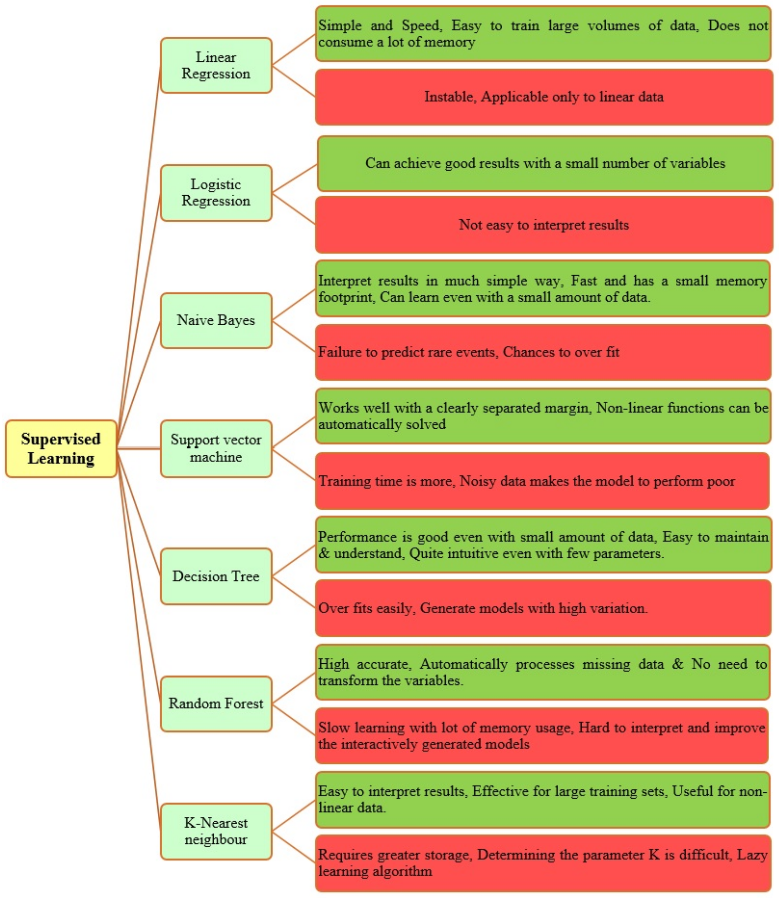
5.4.1. Supervised Learning

Supervised learning is a popular machine learning algorithm used for a dataset that is already labeled. The algorithm is trained through the labeled data to map an input–output relationship. Output can be either a numerical value or classification class. The training data decide the algorithm based on the output that either is a classification or a numerical value.

$${\displaystyle M=\sum _{i=1}^N{X}_i{Y}_i}$$

(23)

where ‘N’ is the number of training samples, ‘$X_i$’ is the multi-dimensional input vector, and ‘$Y_i$’ is the output response. The required work regression or classification decides the algorithm to predict the output. Supervised learning algorithms such as linear regression, multi-linear regression (MLR), logistic regression, K-nearest neighbor (KNN), support vector machine (SVM), decision tree (DT), random forest (RF), extra trees, ensemble learning machine (ELM), gradient boosting (GB), extreme gradient boosting (EGB), and adaptive gradient boosting (AGB) are present. This paper presents some of the popularly used algorithms. An artificial neural network (ANN) combines many processing elements arranged in a sequence of randomly interconnected layers to form a data processing system taken from the methodology involved in the brain’s cerebral cortex. The ANN learns to adjust weights to obtain the accurate output and recalls the weighted adjustment to provide the necessary information [83]. A linear regression model [84] is a frequently used supervised algorithm to establish a linear relationship between two variables. This model predicts output for both regression and classification. When the prediction depends on only one predictor, it is simple regression. The multi-linear regression model uses two or more variables to predict the desired value.

$$Y=mX+C$$

(24)

where ‘Y’ is the output variable, and it depends on the input variable ‘X’ with slope ‘m’. The linear regression model is unable to predict nonlinear data. In such cases, the polynomial regression (PR) model is suggested to estimate the nonlinear data. This model includes a linear regression model and some other independent variables interaction to predict the dependent variable output even from the nonlinearity in the data. The polynomial regression is given by

$$Y={\theta }_0+{\theta }_{1}X+{\theta }_2{X}^2+\dots +{\theta }_n{X}^n$$

(25)

where ‘Y’ is the output variable, and it depends on the input variable ‘X’ with slope or weights ${\theta }_1,{\theta }_2,+\dots +{\theta }_n$, ${\theta }_0$ is the bias or constant term, and ‘n’ is the degree of the polynomial. In addition, ‘n’ determines the suitability for the nonlinear model. The logistic regression (LoR) model is a statistical method based on probability theory mainly used to classify the data. The sigmoid function estimates the probability. The activation function is given by

$$f\left(x\right)=\frac{1}{1+e^{-x}}$$

(26)

The input–output relationship is linear to the small data. The high-dimensional data overfit the model. The predicted output depends on an assumption as linear input–output relationship acts as a drawback to this model. The K-nearest neighbor model (KNN) [85] is a non-parametric decision algorithm to classify or regress the data in a supervised machine learning. This algorithm recognizes the patterns and works well to discriminate patterns in data. The KNN algorithm works classifying the neighborhood points based on Euclidean and Manhattan distance. The ‘K’ value decides the number of neighborhood points taken into account to predict the classification of the data points. If K = 1, the closest neighbor decides the output. If K = 5, the nearest five neighbors’ probabilities calculate the result. The low ‘K’ value underfit and the high ‘K’ value overfit the model, so a proper ‘K’ value is to be chosen to generalize the model. Generally, the ‘K’ value is taken as the square root of a number of samples present in the data. The factors such as K number, size of the training set, and type of metric decide the performance of the K-nearest neighbor.

The decision tree algorithm [86] is a popular classification algorithm that follows the divide-and-conquer strategy similar to a flowchart with each internal node divided into nodes to reach the leaf node. The splitting of the nodes concludes with the leaf node as a solution to the work. The decision node is a split node to divide the tree into branches to reach the best possible result. The root node serves as the base node for the entire tree. The metrics entropy, information gain, gain ratio, and Gini index verify the predicted answer and make the decision tree predict the output accurately. Overgrowth of the tree leads to complexity of the model. The pruning indicates the cutting of unwanted branches and leaves to reduce the complexity and generalize the model. The chi-square test directs the model to remove insignificant nodes in the tree. Many decision trees combine to form an ensemble machine learning random forest model [87] to predict solutions to many regression and classification tasks.

The classification and regression is by the majority in votes and average of values of the prediction models, respectively. The overfitting is a drawback to the decision tree model where the random forest overcomes it. Random forest models can provide accurate results with adjustable changes in the model’s hyper parameters. The extra trees model is extremely randomized decision trees based on score computation. In the decision tree, different splitting rules are applied at each node, and the best split rule is chosen to increase the training speed by making the induction process easy to obtain extra tree model. The major difference between the random forest and extra trees is the selection of a threshold for feature extraction for randomly sampled data. The other difference is no bagging in the extra tree model because the entire dataset is being given to each decision tree to grow, whereas in the random forest, only some random data are used. The changes in the extra trees increase the calculation speed with increased bias and reduced variance compared to other bagging methods. Cortes and Vapnik [88] introduced a support vector machine (SVM) as a machine learning model to solve classification and regression tasks.

The SVM [89] is a popular tool to learn the model by training dataset and gives its effort to generalize the model and predict the required information on new data. The model chooses the finest hyper plane from the training data with +1 and $-1$ as labels with maximum distance from the data points. The model decides the data points based on the features as some data points are behind one label and others are under another label. The name support vectors because the data points close to labels control the hyper plane position.

The hyper plane equation is

$$\omega x+b=0$$

(27)

The model finalizes the solution after minimizing the following equation

$${\displaystyle mi{n}_{\omega ,b}J(\omega ,b)=\frac{1}{2}{\left|\right|\omega \left|\right|}^2+c\sum _{i=1}^n{\delta }_i{\forall }_i[y_i(\omega ,\varphi \left(x_i\right)+b)\ge 1-{\delta }_i]}$$

(28)

where ${\delta }_i\ge 0$, ‘$\omega$’ is the normal vector of the hyperplane or the weights to be updated to set the orientation, ‘b’ is the offset of the hyper plane to the origin, $\varphi \left(x_i\right)$ is the mapping from input space to feature space, and ${\delta }_i$ are the slack variables that permit the non-separable case by allowing misclassification of training instances. A boosting algorithm is an ensemble model that combines different weak models to develop a model with high accuracy. The first model’s output is input to the second model, the second model output to the third model, and the process repeats to obtain the accurate value as a final result. The gradient boosting algorithm [90] learns better than the boosting algorithm by optimizing the loss function by creating a new model with a negative gradient directed to reduce the error in the preceding model. The main drawback of the GBDT algorithm is overfitting the data. To overcome this limitation, some regularization terms were added to the gradient boost algorithm by Chen Tianqi and named as the extreme gradient boost algorithm [91].

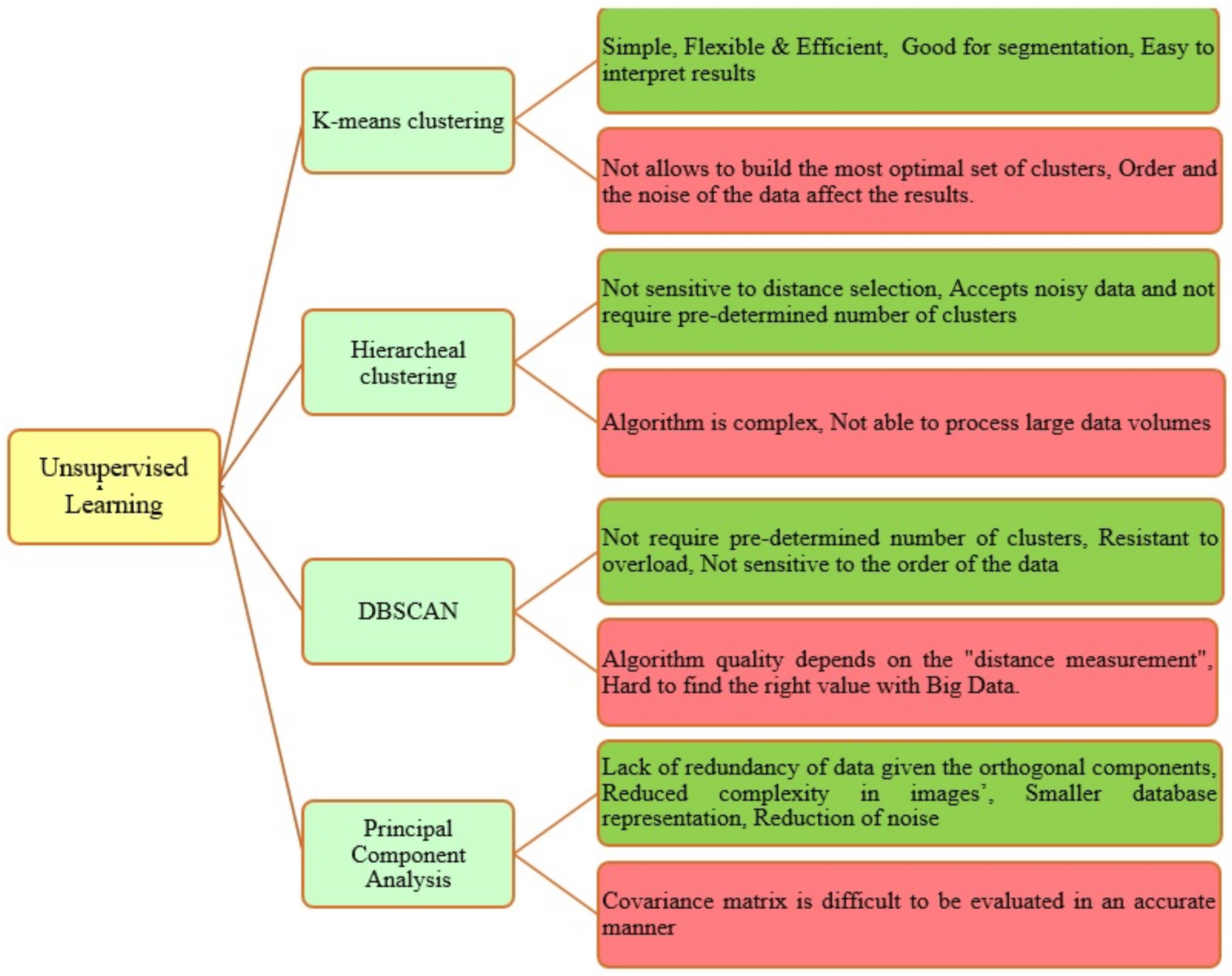
5.4.2. Unsupervised Learning

There should be sufficient knowledge in feature engineering to label data for large datasets. Supervised learning performs the best with labeled data, and unsupervised learning handles the unlabeled data. Unsupervised learning reduces the burden of labeling, and for all tasks, labeled data is not available. The unsupervised algorithms use the raw data as input and detect patterns in the input data to cluster it. These algorithms label the data to feed the labeled data to supervised or semi-supervised learning to achieve good performance in prediction models. Several research improvements in clustering algorithms, principal component analysis (PCA), etc., made unsupervised learning possible in various categorizing applications.

The K-means clustering algorithm [92] is a well-known unsupervised algorithm proposed by MacQueen and rich in clustering the data. K-means clusters the dataset with similarity to the same clusters and dissimilarity to different clusters. The iteration process occurs in the K-means algorithm to find the optimum cluster centers. K-means makes every effort to minimize the squared error difference between the data points and the cluster’s mean in that cluster. The K-means algorithm quickly clusters the large datasets, but the model limits the centroid computation result in local optimum points. The hierarchical clustering is a well-known cluster method that builds a hierarchy of clusters by either combining or dividing the sequence of clusters. There are two popular approaches as agglomerative and divisive algorithms generate an optimum clustered solution in hierarchical clustering. Agglomerative clustering is a bottom-up clustered method that initiates a model with data within singleton clusters and combines clusters in a row to develop a final model with all data in a single cluster or sequence. The most common distance metrics used in agglomerative clustering are single linkage, complete linkage, and average linkage. The single linkage metric usage makes the agglomerative clustering the same as the nearest neighbor clustering model. Divisive clustering is a top-down approach that usually splits the input data into smaller sub classes and iterates until the sub classes split into singleton datasets [93,94].

The DBSCAN algorithm decode clusters based on splitting the high density, medium density, and sparse density data point regions by separate tags. The same cluster samples are closely connected, and if the same category sample data points are high, then it is highly dense; if not it becomes sparse. Two parameters ‘$ϵ$’ and ‘minPts’ play a vital role in the DBSCAN algorithm with one serving as a threshold to consider a data point as a neighbor and the other giving the number of neighbors in the threshold radius respectively. A ‘k’ distance graph helps in finding the ‘$ϵ$’ radius value. These parameters decide the clusters based on the local density of data points in an ‘$ϵ$’ radius region. The minimum minPts to be chosen in the DBSCAN algorithm is three. Mainly three data points are clustered, namely the core point, border point, and the noise point within the ‘$ϵ$’ radius based on minPts number. The principal component analysis (PCA) [30] technique reduces the dimension of multi-featured data by reducing the similarity by converting the samples of correlated features into a new set of samples with uncorrelated features. The PCA [95] is a tool that depicts the geometric properties and reduces similar features in the multivariate statistical data to an unrelated single feature by using matrices.

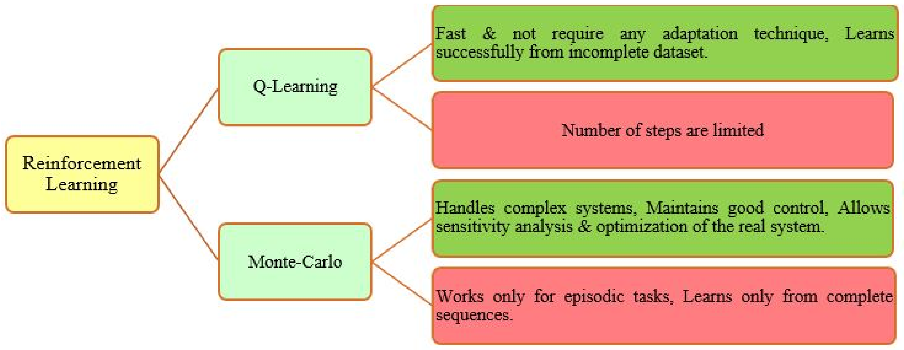
5.4.3. Reinforcement Learning

Reinforcement learning [96] is one of the most popular algorithms in machine learning that makes the object reach the target by rewards and punishments. The RL agent interacts with the information in an uncertain, potentially complex environment and takes the sequence of decisions to reach the objective. The RL model provides the balance between exploitation and exploration. It is a benefit to the RL model compared to supervised models.

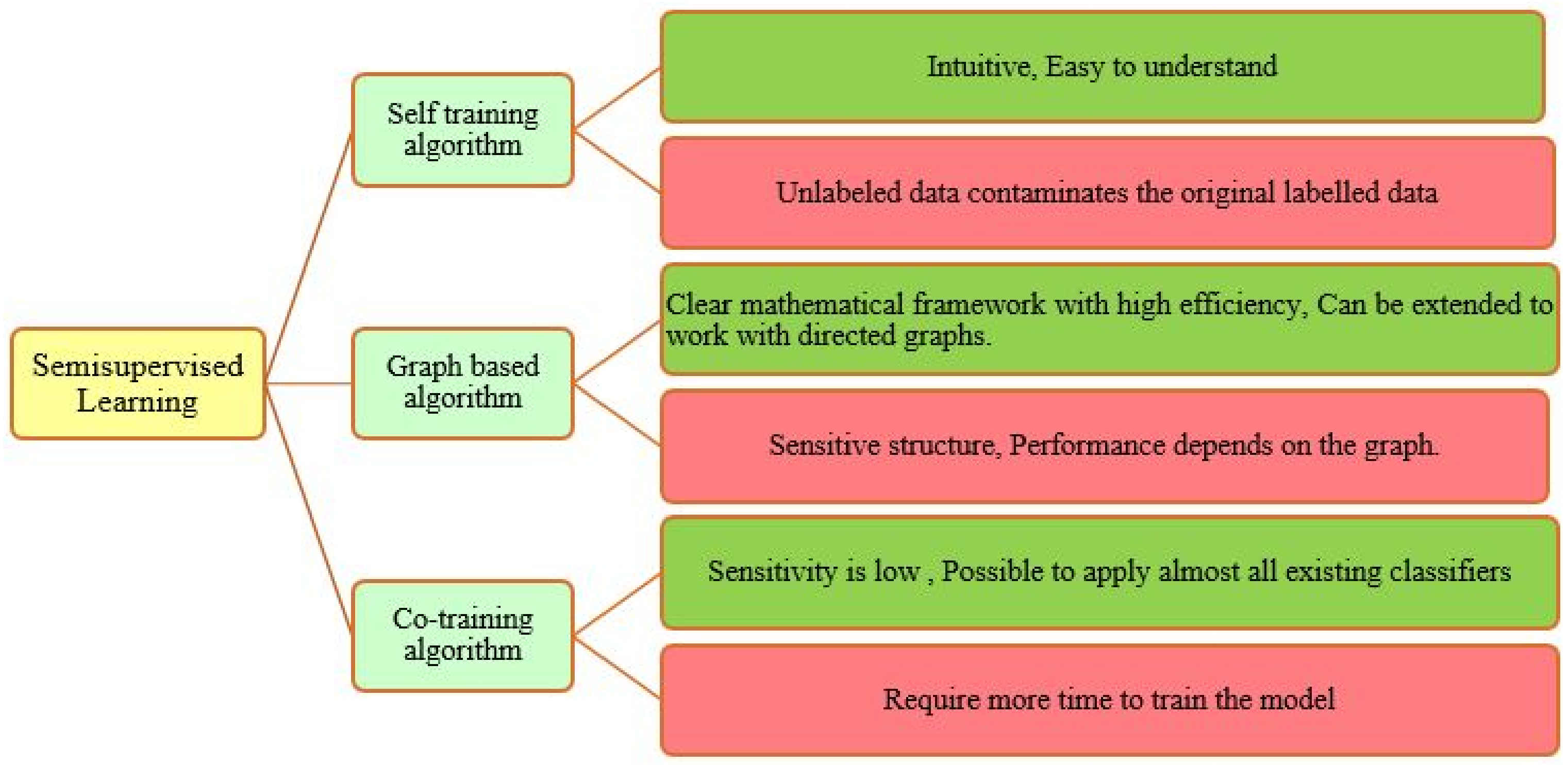
5.4.4. Semi-Supervised Learning

In every case, the complete labeled data are not available, and they price high to collect the labeled dataset. Semi-supervised learning trains the model based on both labeled and unlabeled data. Many models train with the combination of labeled and unlabeled data. Mostly unlabeled data are taken in large quantity compared to labeled data in these models. The metrical summary of the machine learning algorithms such as supervised, unsupervised, etc., for solar energy forecast is shown in

Table 6. Summary of machine learning models.

Reference	Year	Model	Location	Forecast Horizon	Data	Conclusion
Aslam et al.  [97]	2020	FFNN	Seoul/Korea	Hourly	2000 to 2017	RMSE of 109.11 W/m2
Mohammadi et al. [98]	2015	SVM	Bandar Abbas, Iran	Daily and Monthly ahead	1992–2005	MAPE = 3.2601–6.9996%
SANJARI et al. [99]	2017	ANN	Australia	15-min ahead	Two year data 2014 and 2015	CRPS score = 3.81
Marquez et al. [54]	2013	ANN	Davis and Merced, USA	30, 60, 90, and 120 min ahead	1 year (1 January 2011 to 31 January 2012)	RMSE value of 55 to 80 W/m2
Torres et al. [100]	2019	SVR	Oklahoma, USA	3 h ahead	1994 to 2007	MAE = 2225.2 KJ
Wang, J et al. [101]	2018	GBDT	Oregon, USA	1 day ahead	Random 240 day data from the 2015 and 2016 years.	nRMSE varies from 6.96 to 7.72% based on monthly test data
Torres et al. [100]	2019	XGB	Oklahoma, USA	3 h ahead	1994 to 2007	MAE = 2190.9 KJ
Yap et al. [102]	2012	Linear regression	Darwin, Australia	1 h ahead	2008 to 2010	RMSE of 6.72%
Benali et al. [103]	2019	Random Forest	Odeillo, France	hourly	3 years	nRMSE of 19.65% to 27.78%
Liu et al. [104]	2020	SVM	80 sites in China	Daily	1957–2017	$R^2$ = 0.613–0.933 for different sites
Jimenez Perez et al. [105]	2016	EM model	Malaga, Spain	Hourly	2010–2013	rMABE = 15.2%
Basaran et al. [106]	2019	EM model	Afyon, Agri, Sinop, and Hakkari in Turkey	Hourly data	2012–2016	RMSE varies from 4.6–14.6%
Sun et al. [107]	2018	K-means and LSSVM	Beijing, China	Day ahead	2009–2015	MAPE 3.27% to 4.65% from single to multi-step
Bae et al. [108]	2017	SVM RBF	Daejeon, South Korea	1 h ahead	26 months (January 2012 to April 2014)	RMSE = (49.26–62.57) W/m2

.

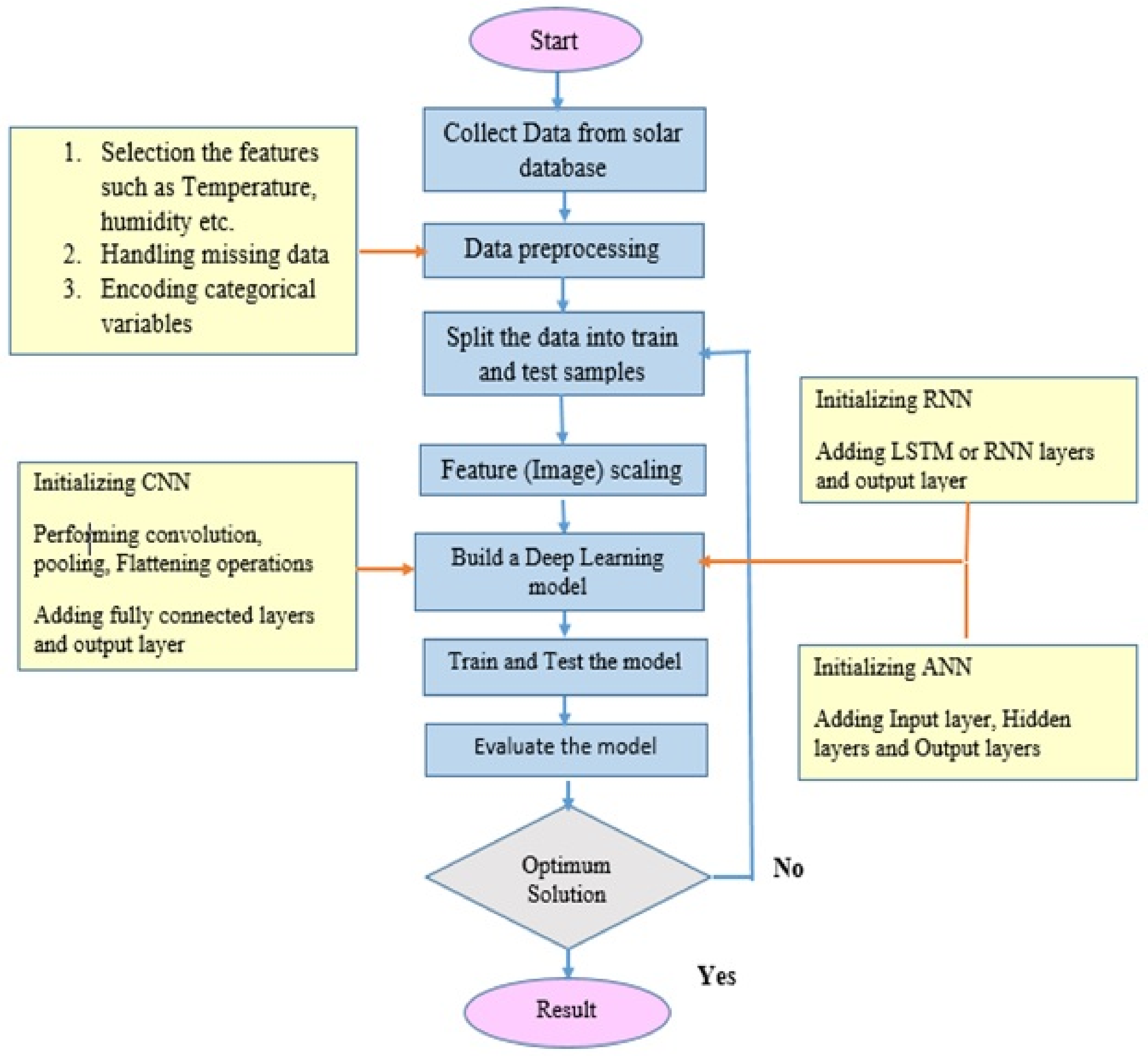
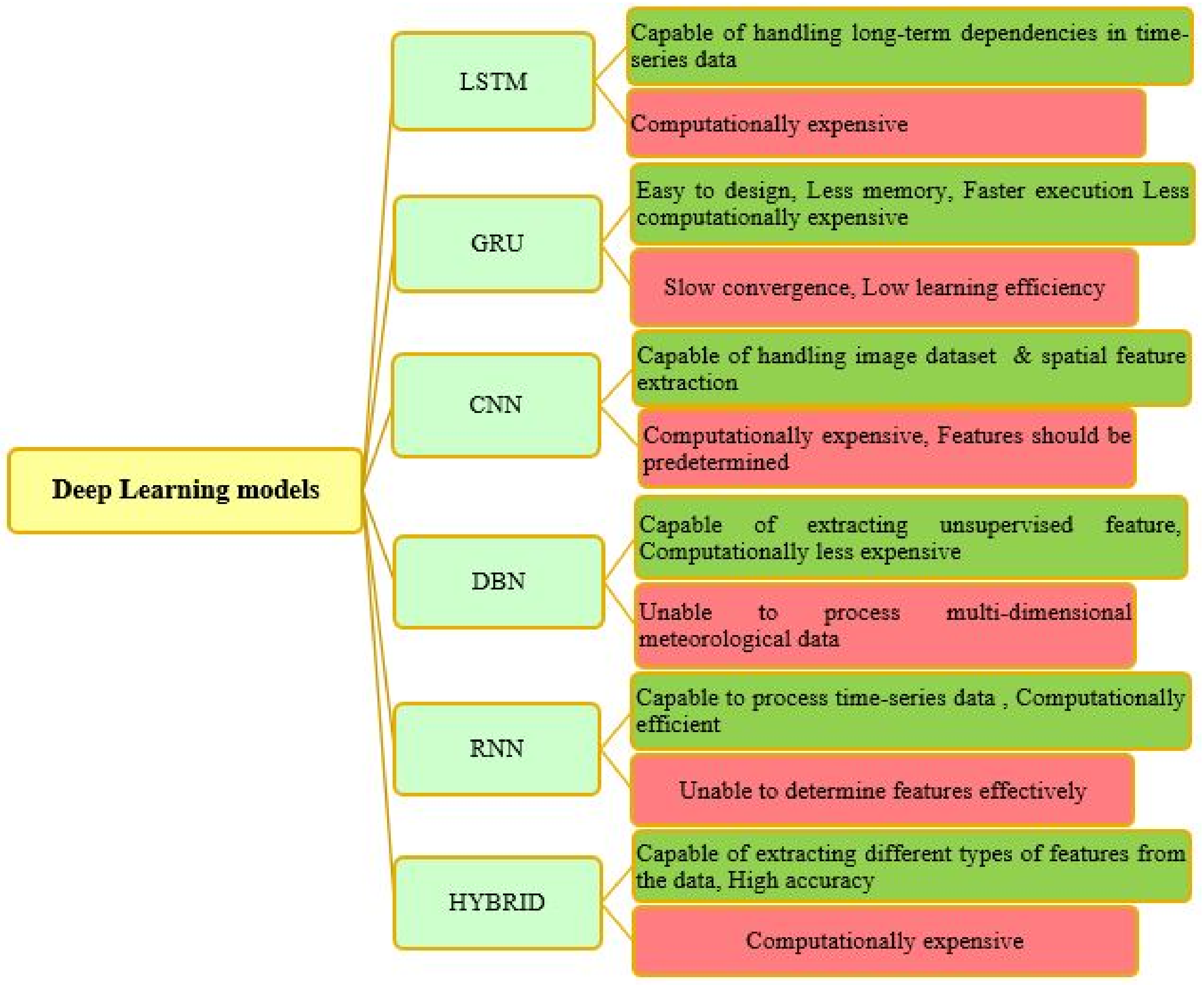
5.5. Deep Learning Models

The input data sometimes contain interconnections and combinations and are not even in the proper structure. To handle datasets of this format through the previous models is not possible. There, we introduce the applications of deep learning, a subset of machine learning. Deep learning models differentiate from machine learning by having a lot of hidden layers by their weights and biases with many activation functions to handle complex datasets. Recent research developments such as long short-term memory, gate recurrent unit, and their combinations proved that the deep learning models predict solar power with accurate results. Figure 14 shows the approach to perform the machine learning models through flowcharts. Figure 15 discusses the merits and demerits of deep learning models.

There are two methods of supervised and unsupervised learning in deep learning. Mainly, three supervised and three unsupervised deep neural networks are discussed in this study.

• Deep multilayer perceptron.
• Convolutional neural networks.
• Recurrent neural networks.
• Auto encoder (AE).
• Restricted Boltzmann Machine (RBM).
• Self-Organizing Maps (SOM).

5.5.1. Supervised Deep Learning

The basic model of DNN is the feed-forward neural network, and here it is named deep multilayer perceptron (DMLP) [110]. DMLP operates through the fully interconnected neuron layers. There is a difference in the number of hidden layers for MLP in DNN compared to ANN architectures. Since the number of hidden layers is high, there will be many more weights, bias, and activation functions in the DMLP infrastructure. The number of neurons in the hidden layer is calculated using empirical formulas during the formulation of the ANN-based model. The formula is given as

$$n=\sqrt{n_i+n_0}$$

(29)

where n is the hidden layer’s neuron number, $n_i$ is the input layer’s neuron number, $n_0$ is the output layer’s neuron number, and an is a bias value ranging from 1 to 10. Computation shows that the hidden layer’s neuron number is set to 60. MLP neural networks [1] are a kind of nonlinear model effective in detecting patterns, modeling, and time series analysis of data. An MLP depends on the data’s structural relationship, a nonlinear mapping between two or more variables. The data supplied to MLP are propagated from the input to the output layer through a hidden layer after the MLP architecture is setup. After the learning phase, the output can be considered assimilated. A suitable learning algorithm minimizes the errors during the training process. It is worth remembering that the MLP model’s learning algorithms depend on the backpropagation approach, which is the steepest gradient descent method. The primary goal of the backpropagation method is to reduce network inaccuracies.

Convolutional neural networks (CNN) [111] are deep learning models that consist of four layers: convolutional, pooling, fully connected, and regression. The convolutional layer contains several convolution filters, each used to create a single feature map. The data can be either a value, image, or video signal. Some algorithms depend on the input dimensions, and they cannot decide the input by feature extraction. Conventional neural networks overcome the disadvantage of detecting features from images with a pooling layer present inside them and perform the best on the multidimensional arrays. The convolutional layer contains several convolution filters, each used to create a single feature map. CNNs also stabilize the neuron layer to layer connections to obtain an accurate prediction. The research developments in graphics and tensor processing units made the CNNs work on large multidimensional data tasks. The function of the pooling layer is to reduce feature map resolution so that input features aggregate. The convolutional layer equation is as follows:

$$y_{i,j,k}^1=F({\left(w_k^1\right)}^T{x}_{i,j}^1+b_k^1)$$

(30)

Maximum and average pooling are the two most used pooling operations. A CNN model [112] is made up of numerous convolutional layers stacked on top of each other, as well as pooling layers. The following function describes the equation of the pooling layers

$$P_{i,j,k}^1=pool(y_{m,n,k}^1)$$

(31)

In most cases, the fully connected layer is beside the regression layer. Every neuron in this layer connects to every neuron from the previous layer in the complete linked layer. The fully connected layer performs the high-level analysis by moving the learned scattered feature representation to one space. The output of the regression layer, which is the final layer of the CNN model, is the final output of the CNN, Zhen et al. and [113] C. Xu et al. [114]. Compared to CNNs and ANNs, the recurrent neural network performs with a different topology. The outputs from the previous state feed as input to the next models in RNNs to capture the temporal features. The gap between RNN and ANN is that RNN uses the last feed-forward’s information generated from its internal state. The RNN uses the Gradient descent algorithm as the back propagation algorithm to solve tasks, but the problem of finding global minima and maxima arises in every case accurately. Gradient vanishing and gradient explosion troubles the RNN in the training phase. Gradient clipping is a simple solution to the gradient explosion problem. Since the gradients are too small to propagate, the gradient vanishing problem makes the model hard to solve. As a result, RNN training performance is not always optimal. The equations for RNN [115] are as follows:

$$S\left(t\right)=\sigma (U^{T}x\left(t\right)+W^{T}S(t-1)+b)$$

(32)

$$y\left(t\right)=\sigma (V^{T}S\left(t\right)+c)$$

(33)

where ‘$x\left(t\right)$’ takes the primary input at time ‘t’. W, U, and V are weight matrices with b and c as constants; ‘$y\left(t\right)$’ is the response at time t, and $\sigma$ is the activation function. Advanced research methods such as long short-term memory (LSTM), and gated recurrent units (GRUs) overcome some of these problems by storing information for a long time and using gate functions. C.-H. Liu et al. [116] Hochreiter and Schmidhuber proposed the long short term memory (LSTM) unit in 1997 as a variant type of RNN. They suggested LSTM as a competent implementation with numerous enhanced modifications. In an LSTM neural network, memory blocks swap the hidden units of an RNN. The essential aspect of LSTM is that it employs an input gate, a forget gate, and an output gate, allowing it to learn what needs to be saved, discarded, and read by regulating the three gates. In LSTM, the previous output first passes through a forget gate, which allows some memory to drop. Then, an input gate injects some additional memories into it. Finally, the output gate processes the final output $y\left(t\right)$. The following equations [117] depict the operation of LSTM units

$$f\left(t\right)=\sigma (w_f^T[h(t-1),x\left(t\right)]+b_f)$$

(34)

$$i\left(t\right)=\sigma (w_i^T[h(t-1),x\left(t\right)]+b_i)$$

(35)

$$g\left(t\right)=Tanh(w_g^T[h(t-1),x\left(t\right)]+b_g)$$

(36)

$$o\left(t\right)=\sigma (w_o^T[h(t-1),x\left(t\right)]+b_o)$$

(37)

$$c\left(t\right)=f\left(t\right)c(t-1)+i_t{g}_t$$

(38)

where ‘w’ and ‘b’ are the weight matrices and biases of associated gates, and $\sigma$ is the activation function. The Bi-LSTM [118] can learn a representation depending on the past and the future and is most sensitive to the input values. It does this by combining another LSTM that moves back to the forward LSTM through the sequence. Therefore, a Bi-LSTM is constructed as multiple inputs on a time scale and produces a series of vectors as output, Dabbagh Manesh et al. [119] Z. Huang et al. [120]. The gate recurrent unit (GRU) is a variant of RNN that uses a gating mechanism to maintain past inputs in the networks’ internal state to process sequential data memories and map them from the previous input history to target vectors. The GRU has fewer gates than the LSTM. Because the GRU merges the input and forget gates into a single gate named the update gate. Two major gates in the GRU are the update gate and the reset gate. The update gate regulates the data from the previous state to the current state. The reset gate governs the ignored past information from the GRU to the present moment. The equations [114] are as follows

$$Z\left(t\right)=\sigma (w_z^{T}x\left(t\right)+w_z^{T}h(t-1))$$

(39)

$$R\left(t\right)=\sigma (w_r^{T}x\left(t\right)+w_r^{T}h(t-1))$$

(40)

$$h\left(t\right)=Tanh(w_h^{T}x\left(t\right)+w_h^t(r\left(t\right)⨀h(t-1)))$$

(41)

$$h\left(t\right)=(1-z\left(t\right))h(t-1)+z\left(t\right)\widetilde{h\left(t\right)}$$

(42)

The present GRU algorithm, on the other hand, has two flaws. The first is that preprocessing data packets for network packets requires a lot of manual work, and the second is that memory utilization is excessive.

5.5.2. Unsupervised Deep Learning

This algorithm does not require tags to predict the output in training the model. Without any supervision, these models detect patterns of hidden structures in the input data to clusters.

An auto encoder (AE) [121] transforms the input latents before feeding them to a decoder for reconstruction at the output. The significant property of AEs is that they have the same training goal as the input.

$$h^{SP}=f(W_{e}SP+b_e)$$

(43)

$$S{P}_d=d\left(W_d{h}^{SP}\right)+b_d$$

(44)

where ‘$h^{SP}$’ is the encoder operator of the solar power input, and ‘$S{P}_d$’ is the decoder operator of AE and $h^{SP}$. ‘$W_d$’ and ‘$W_e$’ are the weight matrixes with biases ‘$b_d$’ and ‘$b_e$’ of decoder and encoder, respectively.

The output characteristic equation

$$O_i=f(W_0.(h_i^{SP}+S{P}_{d,i})+b_0)$$

(45)

The function of activation function gives the desired output

$$Y_i=g(W_y.O_i+b_y)$$

(46)

The restricted Boltzmann machine (RBM) is a generative model that maps the predictions across training datasets using a stochastic distribution. RBMs can be used to speed up training with bipartite graphs of neural interconnections. The RBMs are stacked together to build deep Boltzmann machines. The DBMs are often used as feature detectors to generate representations from data. Supervised learning is further used in fine-tuning network weights and improving performance on specific learning tasks. The self-organizing map (SOM) [122] represents a one- or two-dimensional dataset from a higher dimensional dataset without any change in the topological structure of the dataset. The SOM architecture has an input and an output layer. The neurons in the input layer are connected fully to the output layer neurons. The neurons in the output layer compete one-to-one to result in the best matching unit by the smallest Euclidean distance from the input vector. The Euclidean distance is given by

$$E_d=\sqrt{{\displaystyle \sum _{k=0}^K{(x_k-w_{ik})}^2}}$$

(47)

The SOM groups the nodes based on the similarity concerning the best matching unit. The ordering phase of SOM decides the BMU, and the adjustment phase adjusts the radius of the BMU to achieve the optimum solution. The weight adjustment is given by

$$w_{ik}\left(n\right)=w_{ik}(n-1)+\delta (x_x\left(n\right)-w_{ik}(n-1))$$

(48)

For all, $i=1,2,\dots ,T,k=1,2,\dots$

where ‘$x_k$’ is the kth component of the input vector ‘x’, J is the dimension of the input vector ‘x’, ‘T’ is the total number of neurons in the output layer, and ‘$\delta$’ is the learning rate parameter. Following Kohonen’s rule, the weights given to the BMU and its neighbors are driven to migrate toward the input vector supplied to the network, resulting in a reduced Euclidean distance and assisting them to group similar vectors. The computational summary of the deep learning models are presented in

Table 7. Summary of deep learning models.

Reference	Year	Model	Location	Forecast horizon	Data	Conclusion
Voyant et al. [73]	2014	MLP	Mediterranean, France	24 h ahead	10 years data	nRMSE ranges from 28.6 to 31.9%
F. Wang, et al. [115]	2020	BPNN	Nevada.	Day-ahead	2011 to 2016	RMSE of 10.31%
C. Fang et al. [123]	2020	CNN	Golden, Colorado, USA	10 min ahead	Ten years data 1 January 2008 to 31 December 2017	RMSE of 80.14 W/m2
Yuchi Sun et al. [124]	2019	CNN	USA	15 min ahead	1 year (March 1st 2017 to March 1st 2018)	RMSE: 2.1 kW/25 kW
S. Mishra et al. [125]	2018	RNN	Boulder, Desert Rock, Fort Peck, Sioux Falls, Bondville, Goodwin Creek, and Penn State	1, 2, 3 and 4 h ahead	2009, 2010, 2011, 2015, 2016 and 2017 year data	Mean RMSE of 9.713 to 39.812%
Yu et al. [126]	2019	LSTM	Atlanta, New York, and Hawaii in USA.	1 h ahead	2013 to 2017	RMSE in a range of 45.84 W/m2 and 41.37 W/m2 in two different locations.
Qing et al. [127]	2018	LSTM	Santiago, Cape Verde.	1 h ahead	2.5 years (March 2011 to August 2012 and January 2013 to December 2013)	RMSE value of 76.245 W/m2
Chandola et al. [128]	2020	LSTM	Arid zones of India	3, 6, 24 h ahead	Five years dataset (2010 to 2014)	MAPE values ranging 6.79% to 10.47%.
Jeon and Kim [129]	2020	LSTM	Korea Meteorological Administration.	24 h ahead	1825 days	RMSE of 30 W/m2
Obiora et al. [130]	2020	LSTM	Johannesburg city	1 h ahead	Ten years data 2009 and 2019	Improvement of 3.2% NRMSE over the SVR model
Mukherjee et al. [131]	2018	LSTM	Kharagpur, India	1 h ahead	Fifteen years of recorded data from 2000 to 2014	RMSE value of 57.249 W/m2
Justin et al. [132]	2020	LSTM	Weather station, Rizal	Any time	Six months data (September 2019 to February 2020)	$R^2$ value 0.953 and MAE value 41.738 W/m2
A. Rai et al. [133]	2021	GRU	New Delhi, India	24 h, 48 h, and 360 h	31-December–2015 to 31–December–2016	MAE of 0.0321, 0.0332 and 0.0377

.

5.6. Probabilistic Models

This paper discusses basic probabilistic models [134] such as Gaussian distribution, quantile regression, etc. Gaussian distribution [135] depends on training and testing datasets to forecast solar power with allowable variance. In this case, the probability integral transform evaluates the probability distribution. The quantile regression [136] is a popular regression model for solar power estimation. The QR model individually minimizes the cost function of each quantile. These models use historical data to estimate the output. The literature survey on probabilistic models are analyzed and summarized in

Table 8. Summary of special artificial intelligence models.

Reference	Year	Model	Location	Forecast Horizon	Data	Conclusion
M. Russo et al.  [68]	2014	Genetic Algorithm	ENEL Catania site, Italy	15 min	1 whole year 2010	RMSE: 67.6 W/1000 W
S.Garg et al. [137]	2020	Markov Chains	Bhadla, Jodhpur, Rajasthan, India	Day ahead	5 years (2010–2014)	MAPE value of 5.04 to 26.56 varies from month to month.
V. Gunasekaran et al. [91]	2021	Genetic Algorithm	Bondville IL, Pennstate, PA and Desertrock, NV.	1 min. ahead GHI	2018 to 2020	MAE of 4.64, 3.08 and 4.58 respectively
Yona et al.  [138]	2013	Fuzzy Logic	Okinawa, Japan	24 h ahead	1 year of data	Average MAE of 0.22

.

5.7. Special AI Models

Y.WANG et al. [139] Theoretically, BPNN can estimate any nonlinear function with high precision. The most significant drawback of BPNN is that it may reach a local optimum owing to recurrent calculations. The genetic algorithm (GA) [140] solves these challenges and brings the result to a global optimum. The GA is a stochastic searching strategy that can find the best value rapidly and precisely, Yuqi Tao [141]. The authors considered the operating parameters such as the population number ‘N’, the generation of evolution ‘gen’, the crossover operator ‘PC’, and the mutation operator ‘PM’. The coding starts with initiating the population with weight lengths and thresholds through coding. The initialized weights and thresholds in BP are encoded to read and normalize them. The absolute error between the predicted output and the desired output of the BP network serves as the fitness value. Finally, the operations such as selection, crossover, and mutation provide the optimal weights and thresholds of the model to yield its best optimal solution.

B Gururaj et al. [142] proposed fuzzy logic that had been examined as infinite-valued logic in the 1920s by Tarski et al. Lotfi Zadeh introduced the term fuzzy logic in 1965. Fuzzy sets are mathematical representations of ambiguity and inaccuracy. These models are capable of identifying, expressing, manipulating, and interpreting. Probability provides only either true or false as two conclusions, but fuzzy logic provides the degree of truth. Fuzzification, inference, and de-fuzzification are the three parts of fuzzy logic. The authors investigated many applications of fuzzy logic. In one approach, the fuzzy technique was used for three locations in India to estimate monthly averages of daily irradiances. It is also recommended to add other meteorological variables to the conditional statements in the fuzzy implications employed in this approach to improve the precision of solar irradiation estimation in that approach. A Markov chain [143] technique that models the transition probabilities between discrete power levels generates probabilistic forecasts without assuming a distributional geometry. These models are reviewed analytically and mathematically in

Table 9. Summary of probabilistic models.

Reference	Year	Model	Location	Forecast Horizon	Data	Conclusion
Mitrentsis et al.  [144]	2021	Natural Gradient Boosting	Germany	day-ahead	February 2018 to October 2019	RMSE of 5.77 to 6.17% from reduced to full features
S. Alessandrini et al. [145]	2015	Quantile Regression	Milano, Catania, and Calabria in Italy	0–72-h ahead	January 2010 to December 2011 (Catania), July 2010 to December 2011 (Milano), and April 2011 to March 2013 (Calabria)	CATANIA MRE = 5.92% CALABRIA MRE = 7.72% MILANO MRE = 8.03%
DOUBLEDAY et al. [146]	2021	Bayesian Model Averaging	Texas	1, 4, 12, and 24 h ahead	Two-plus years of data November 2016 to December, 2018.	CRPS score of 5.18 to 7.47 varies from site to site.
KHODAYAR et al. [147]	2020	Convolutional Graph Auto encoder	USA	30-min up to 6 h ahead GHI	1998 up to 2016	CGAE obtains 2.53% better CRPS than ST-QR-Lasso

.

5.8. Hybrid & Ensemble Machine Learning Models

X. Huang et al. [148] examined hybrid models that have received much interest since they can combine the benefits of many approaches. Model combination in forecasting depends on using each model’s distinct feature to catch different patterns in the data. The ensemble machine learning model boosts various weak learners to strong models with an acceptable level of variance and bias. The drawback of overfitting the decision tree model occurs because of the repetition process in the concluding leaf node. There are many methods such as pruning, random forest, extra trees, etc. to overcome this limitation. The hybrid and the ensemble models are mathematically summarized in

Table 10. Summary of hybrid models.

Reference	Year	Model	Location	Forecast Horizon	Data	Conclusion
SANJARI et al.  [99]	2017	Markov Chain, Gaussian mixture and Genetic algorithm	Australia	15-min ahead	Two year (2014 and 2015)	CRPS 2.16
Yona et al.  [138]	2013	Fuzzy theory, RNN	Okinawa, Japan	24 h head	1 year of data	Average MAE of 0.1327
Voyant et al. [53]	2012	ANN and ARMA	Mediterranean, France	1 h ahead	6 years data	average nRMSE is 14.9%
Marzouq et al. [54]	2013	GA-MLP	Fez in Morocco	Daily	7 years (2009 to 2015	$R^2$ = 0.975
Perveen et al. [149]	2019	ANFIS	India	10 min ahead	15 years (2002 to 2016)	Average MAPE = 0.00000021%
Chen et al  [150]	2013	Fuzzy logic, MLP	Singapore	Hourly	One month	MAPE = 6.03–9.65%
Yeom et al.  [151]	2020	CNN- LSTM network	Korean Peninsula.	1 h ahead	1 April 2011 to 31 December 2015	RMSE value of 71.334 W/m2 and $R^2$ value of 0.895.
D. Yang et al. [152]	2021	AnEn+LPQR	Oahu Solar Measurement Grid, Hawaii.	4 s to 1 min ahead	2010 March to 2011 October	CRPS score of 24.7 to 64.5 and Average skill score is 27.80%
A. Rai et al. [133]	2021	AE-GRU	New Delhi, India	24 h, 48 h, and 360 h ahead	1 year (31-December–2015 to 31–December–2016)	$R^2$ Coefficient of 0.8976247 to 0.937336
F. Wang, et al. [115]	2020	LSTM-RNN	Nevada.	Day-ahead	6 years (2011 to 2016)	RMSE value of 8.83%
ZHANG et al. [153]	2021	Federated BayesLSTM-NN	Ningxia, China	Intra hour, Intraday and day ahead	July 2006 to November 2018	MAE of 49.1, 53.1 and 71.6 W/m2
Ratshilengo et al. [38]	2019	GA-SVM	Victoria, Australia	1 h ahead	278 days	RMSE of 11.226 W and MAPE of 1.70%
Jing Bi et. Al [154]	2021	Wavelet Transformation—LSTM	US Virgin Islands	5 min.	19 October 2013 to 19 November 2013	$R^2$= 0.98
Jing Bi et. Al [154]	2021	Wavelet Transformation—BPNN	US Virgin Islands	5 min.	19 October 2013 to 19 November 2013	$R^2$ = 0.99
Jing Bi et. Al [155]	2022	ST-LSTM	Spanish Wikipedia	1 h	1 July 2015 to 1 July 2016.	$R^2$ = 0.99
M. Ghayekhloo [156]	2015	Game Theory (GT)-SOM	Ames, Iowa, United States	1 h, 2 h, 3 h and 1 day ahead	2011 and 2013	RMSE value of 67.921, 82.506, 113.4 and 119.75 W/m2 respectively
Monjoly et. Al [79]	2017	WD–AR	Le Raizet, France	1 h	January 2012 to December 2013	RMSE value of 19.57%
Monjoly et. Al [79]	2017	WD–AR–ANN	Le Raizet, France	1 h	January 2012 to December 2013	RMSE value of 7.90%

and

Table 11. Summary of ensemble learning models.

Reference	Year	Model	Location	Forecast Horizon	Data	Training/Test Split Ratio	Conclusion
Yongqi Liu et al. [5]	2019	CNN and GRU	United States	3 h-ahead GHI	2 years (1 January 2013 to 31 December 2014)	8760 h / 8760 h	Mean RMSE of 69.5 W/m2
Davide Cannizzaro et al. [157]	2021	Convolutional Neural Networks (CNN) and Random Forest (RF)	University Campus in Turin, Italy,	Next 15 min up to next 24 h GHI	December 2009 to November 2015	(6 years) December 2009 to November 2014/December 2014 to November 2015	$R^2$ coefficient of 0.936 to 0.908
Davide Cannizzaro et al. [157]	2021	Convolutional Neural Networks (CNN) and Long Short Term Memory (LSTM)	University Campus in Turin, Italy	Next 15 min up to next 24 h GHI	December 2009 to November 2015 with a time- resolution of 15 min (6 years)	December 2009 to November 2014/December 2014 to November 2015	$R^2$ coefficient of 0.937 to 0.908
Pratima Kumari et al. [158]	2020	Extreme gradient boosting forest and Deep neural networks (XGBF-DNN)	New Delhi, Jaipur and Gangtok in India	1 h GHI ahead	Ten years (from 2005 to 2014)	First eight years of data/Two years of data.	RMSE of 56.68 W/m2, 53.78 W/m2 and 91.86 W/m2 of Jaipur, New Delhi, and Gangtok respectively.
Nonita Sharma et al. [159]	2021	Long Short Term Memory (LSTM) Layer and Maximal Overlap Discrete Wavelet Transform (MODWT)	Yulara Solar System, Australia	1 day, 10 days, and 1 month ahead GHI	January 2016 (12:00:00 a.m.) to 10 June 2020 (4:50:00 a.m.)	2016–2019/2020	RMSE of 0.1109, 0.1231, and 0.1231 kW for 1 day, 10 days, and 1 month, respectively
Fermín Rodríguez et al. [160]	2021	Feed forward neural network and a Spatio-temporal approach	Vitoria–Gasteiz, Spain	10 min ahead GHI	2015–2017 (3 years)	2015–2016/2017	RMSE of 50.80 W/m2
Waqas Khan et al. [161]	2021	DSE-XG (ANN, LSTM and XGBoost)	Bunnik, Netherlands	15 min and 1 h ahead GHI	2016 to 2019 years data by solar gis	Four folds/One fold	RMSE of 0.35, and 0.26 kW for 15 min. and 1 h respectively
Liping Liu et al. [104]	2019	SVM, MLP and MARS	Australia Solar Centre (DKASC), Australia	1 day ahead GHI	15 August 2013 up to 17 June 2018	4 months of each year (from 2014 to 2018), with a total of 600/4 days in 2018	RMSE of 0.1248 to 0.53 kW

, respectively.

The results of various forecast models are compared and the paper is summarized by the conclusion as shown in Figure 16.

Table 12. Colour code representation of represented mapping’s in Figure 16.

Horizon Mostly Used—Model	Source—Model
Very short term—Blue—1,4,6,8	Geographical & Meteorological data—Blue—1,3,8
Short term—Brown—2,3,4,5,6,7,8	Cloud & Satellite Imagery data—Brown—2,8
Medium term—Black—3,4,6,8	NWP data—Black—2,3,4,6,7,8
Long term—Green—2,3,8	Historical data—Green—3,4,5,6,7,8
Error evaluation—Violet	Real time monitoring data—2,8

makes the clear view to understand the pictorial conclusion.

6. Conclusions

This paper explains more than 100 models by their characteristics and metric performance with additionally adding merits and drawbacks of each. The solar irradiance and power forecast model classifications made in this paper allow the researcher to analyse each model in an effective perspective. It also helps find the best model suited for a particular location with a preferred time horizon. The huge amount of nonlinear and non-stationary data influenced the artificial intelligence models to use in predicting the best results. The AI models are broadly classified into three separate groups, namely machine learning, deep learning, and special AI models in the review to enhance a clear view of solar energy forecasting. Some important metrics are briefly explained in our paper to understand each model explained. The deep learning models provide the information to the researcher to use images from satellites and the sky to estimate solar energy more efficiently. Nearly 70 models are compared with the time interval, spatial area, and the metrics, and nearly 30 models are surveyed theoretically. This helps the researcher understand the forecast models from the beginning to recent years. The latest research developments mentioned clearly show the priority of ensemble and hybrid models over other models. Comparing all the models, the ensemble and hybrid models provide better prediction with required time horizon from minutes to several days.

References

1. Lima, M.; Carvalho, P.; Fernández-Ramírez, L.; Braga, A. Improving solar forecasting using Deep Learning and Portfolio Theory integration. Energy 2020, 195, 117016. [Google Scholar] [CrossRef]
2. Alkhayat, G.; Mehmood, R. A Review and Taxonomy of Wind and Solar Energy Forecasting Methods Based on Deep Learning. Energy AI 2021, 4, 100060. [Google Scholar] [CrossRef]
3. Ahmed, R.; Sreeram, V.; Mishra, Y.; Arif, M. A review and evaluation of the state-of-the-art in PV solar power forecasting: Techniques and optimization. Renew. Sustain. Energy Rev. 2020, 124, 109792. [Google Scholar] [CrossRef]
4. Marino, C.; Nucara, A.; Panzera, M.F.; Pietrafesa, M.; Pudano, A. Economic Comparison Between a Stand-Alone and a Grid Connected PV System vs. Grid Distance. Energies 2020, 13, 3846. [Google Scholar] [CrossRef]
5. Liu, Y.; Qin, H.; Zhang, Z.; Pei, S.; Wang, C.; Yu, X.; Jiang, Z.; Zhou, J. Ensemble spatiotemporal forecasting of solar irradiation using variational Bayesian convolutional gate recurrent unit network. Appl. Energy 2019, 253, 113596. [Google Scholar] [CrossRef]
6. Pazikadin, A.; Rifai, D.; Ali, K.; Malik, M.; Abdalla, A.; Faraj, M. Solar irradiance measurement instrumentation and power solar generation forecasting based on Artificial Neural Networks (ANN): A review of five years research trend. Sci. Total Environ. 2020, 715, 136848. [Google Scholar] [CrossRef] [PubMed]
7. Akhter, M.N.; Mekhilef, S.; Mokhlis, H.; Mohamed Shah, N. Review on forecasting of photovoltaic power generation based on machine learning and metaheuristic techniques. IET Renew. Power Gener. 2019, 13, 1009–1023. [Google Scholar] [CrossRef]
8. Singh, I. Solar Power Forecasting: A Review. Int. J. Comput. Appl. 2016, 145, 28–50. [Google Scholar] [CrossRef]
9. Yang, B.; Zhu, T.; Cao, P.; Guo, Z.; Zeng, C.; Li, D.; Chen, Y.; Ye, H.; Shao, R.; Shu, H.; et al. Classification and summarization of solar irradiance and power forecasting methods: A thorough review. CSEE J. Power Energy Syst. 2021. [Google Scholar] [CrossRef]
10. Wang, J.; Zhong, H.; Lai, X.; Xia, Q.; Wang, Y.; Kang, C. Exploring Key Weather Factors From Analytical Modeling Toward Improved Solar Power Forecasting. IEEE Trans. Smart Grid 2017, 10, 1417–1427. [Google Scholar] [CrossRef]
11. Sreekumar, S.; Bhakar, R. Solar Power Prediction Models: Classification Based on Time Horizon, Input, Output and Application. In Proceedings of the 2018 International Conference on Inventive Research in Computing Applications (ICIRCA), Coimbatore, India, 11–12 July 2018; pp. 67–71. [Google Scholar] [CrossRef]
12. Gupta, P.; Singh, R. PV power forecasting based on data-driven models: A review. Int. J. Sustain. Eng. 2021, 14, 1733–1755. [Google Scholar]
13. Antonanzas, J.; Osorio, N.; Escobar, R.; Urraca, R.; Ascacibar, F.J.; Antonanzas, F. Review of photovoltaic power forecasting. Solar Energy 2016, 136, 78–111. [Google Scholar] [CrossRef]
14. Huang, R.; Huang, T.; Gadh, R.; Li, N. Solar generation prediction using the ARMA model in a laboratory-level micro-grid. In Proceedings of the 2012 IEEE Third International Conference on Smart Grid Communications (SmartGridComm), Tainan, Taiwan, 5–8 November 2012; pp. 528–533. [Google Scholar] [CrossRef]
15. Prado-Rujas, I.I.; García-Dopico, A.; Serrano, E.; Pérez, M.S. A Flexible and Robust Deep Learning-Based System for Solar Irradiance Forecasting. IEEE Access 2021, 9, 12348–12361. [Google Scholar] [CrossRef]
16. Mayer, M.; Grof, G. Extensive comparison of physical models for photovoltaic power forecasting. Appl. Energy 2020, 283, 116239. [Google Scholar] [CrossRef]
17. Ayvazoğluyüksel Erol, Ö.; Başaran Filik, Ü. Estimation methods of global solar radiation, cell temperature and solar power forecasting: A review and case study in Eskişehir. Renew. Sustain. Energy Rev. 2018, 91, 639–653. [Google Scholar] [CrossRef]
18. Singh, B.; Pozo, D. A Guide to Solar Power Forecasting using ARMA Models. In Proceedings of the 2019 IEEE PES Innovative Smart Grid Technologies Europe (ISGT-Europe), Bucharest, Romania, 29 September–2 October 2019; pp. 1–4. [Google Scholar] [CrossRef]
19. Mbaye, A.; Ndiaye, M.; Ndione, D.; Diaw, M.; Traore, V.; Amadou, N.; Sylla, M.; Aidara, M.; Diaw, V.; Traoré, A.; et al. ARMA model for short-term forecasting of solar potential ARMA model for short-term forecasting of solar potential: Application to a horizontal surface on Dakar site A. Mbaye et al, ARMA model for short-term forecasting of solar. OAJ Mat. Dev. 2019, 4, 1–8. [Google Scholar]
20. As’ad, M. Finding the Best ARIMA Model to Forecast Daily Peak Electricity Demand. In Proceedings of the Fifth Annual ASEARC Conference-Looking to the Future-Programme and Proceedings, Hong Kong, 2–3 February 2012; p. 12. [Google Scholar]
21. Colak, I.; Yesilbudak, M.; Genc, N.; Bayindir, R. Multi-period Prediction of Solar Radiation Using ARMA and ARIMA Models. In Proceedings of the 2015 IEEE 14th International Conference on Machine Learning and Applications (ICMLA), Miami, FL, USA, 9–11 December 2015; pp. 1045–1049. [Google Scholar] [CrossRef]
22. Li, Y.; Su, Y.; Shu, L. An ARMAX model for forecasting the power output of a grid connected photovoltaic system. Renew. Energy 2014, 66, 78–89. [Google Scholar] [CrossRef]
23. Guo, G.; Wang, H.; Bell, D.; Bi, Y.; Greer, K. KNN Model-Based Approach in Classification. Lect. Notes Comput. Sci. 2003, 2888, 986–996. [Google Scholar] [CrossRef]
24. Leva, S.; Dolara, A.; Grimaccia, F.; Mussetta, M.; Ogliari, E. Analysis and validation of 24 hours ahead neural network forecasting of photovoltaic output power. Math. Comput. Simul. 2015, 131, 88–100. [Google Scholar] [CrossRef]
25. Ahmad, M.; Mourshed, M.; Rezgui, Y. Tree-based ensemble methods for predicting PV power generation and their comparison with support vector regression. Energy 2018, 164, 465–474. [Google Scholar] [CrossRef]
26. Feng, C.; Cui, M.; Hodge, B.M.; Lu, S.; Hamann, H.F.; Zhang, J. Unsupervised Clustering-Based Short-Term Solar Forecasting. IEEE Trans. Sustain. Energy 2019, 10, 2174–2185. [Google Scholar] [CrossRef]
27. Hashemi, B.; Cretu, A.M.; Taheri, S. Snow Loss Prediction for Photovoltaic Farms Using Computational Intelligence Techniques. IEEE J. Photovolt. 2020, 10, 1044–1052. [Google Scholar] [CrossRef]
28. Pan, C.; Tan, J. Day-Ahead Hourly Forecasting of Solar Generation Based on Cluster Analysis and Ensemble Model. IEEE Access 2019, 7, 112921–112930. [Google Scholar] [CrossRef]
29. Zhang, J.; Zhang, Y. Forecast of photovoltaic power generation based on DBSCAN. E3S Web Conf. 2021, 236, 02016. [Google Scholar] [CrossRef]
30. Chahboun, S.; Maaroufi, M. Principal Component Analysis and Machine Learning Approaches for Photovoltaic Power Prediction: A Comparative Study. Appl. Sci. 2021, 11, 7943. [Google Scholar] [CrossRef]
31. Xiu, J.; Zhu, C.; Yang, Z. Prediction of solar power generation based on the principal components analysis and the BP neural network. In Proceedings of the 2014 IEEE 3rd International Conference on Cloud Computing and Intelligence Systems, Shenzhen, China, 27–29 November 2014; pp. 366–369. [Google Scholar] [CrossRef]
32. Shojaeighadikolaei, A.; Ghasemi, A.; Bardas, A.G.; Ahmadi, R.; Hashemi, M. Weather-Aware Data-Driven Microgrid Energy Management Using Deep Reinforcement Learning. In Proceedings of the 2021 North American Power Symposium (NAPS), College Station, TX, USA, 14–16 November 2021; pp. 1–6. [Google Scholar] [CrossRef]
33. Huang, C.J.; Kuo, P.H. Multiple-Input Deep Convolutional Neural Network Model for Short-Term Photovoltaic Power Forecasting. IEEE Access 2019, 7, 74822–74834. [Google Scholar] [CrossRef]
34. Alzahrani, A.; Shamsi, P.; Dagli, C.; Ferdowsi, M. Solar Irradiance Forecasting Using Deep Neural Networks. Procedia Comput. Sci. 2017, 114, 304–313. [Google Scholar] [CrossRef]
35. Liu, J.; Fang, W.; Zhang, X.; Yang, C. An Improved Photovoltaic Power Forecasting Model with the Assistance of Aerosol Index Data. IEEE Trans. Sustain. Energy 2015, 6, 1–9. [Google Scholar] [CrossRef]
36. Wen, S.; Zhang, C.; Lan, H.; Xu, Y.; Tang, Y.; Huang, Y. A Hybrid Ensemble Model for Interval Prediction of Solar Power Output in Ship Onboard Power Systems. IEEE Trans. Sustain. Energy 2021, 12, 14–24. [Google Scholar] [CrossRef]
37. Lu, H.; Chang, G. A Hybrid Approach for Day-Ahead Forecast of PV Power Generation. IFAC-PapersOnLine 2018, 51, 634–638. [Google Scholar] [CrossRef]
38. Ratshilengo, M.; Sigauke, C.; Bere, A. Short-Term Solar Power Forecasting Using Genetic Algorithms: An Application Using South African Data. Appl. Sci. 2021, 11, 4214. [Google Scholar] [CrossRef]
39. Ospina, J.; Newaz, A.; Faruque, M.O. Forecasting of PV plant output using hybrid wavelet-based LSTM-DNN structure model. IET Renew. Power Gener. 2019, 13, 1087–1095. [Google Scholar] [CrossRef]
40. Li, G.; Xie, S.; Wang, B.; Xin, J.; Li, Y.; Du, S. Photovoltaic Power Forecasting With a Hybrid Deep Learning Approach. IEEE Access 2020, 8, 175871–175880. [Google Scholar] [CrossRef]
41. Jalali, S.M.J.; Khodayar, M.; Ahmadian, S.; Shafie-khah, M.; Khosravi, A.; Islam, S.M.S.; Nahavandi, S.; Catalão, J.P.S. A New Ensemble Reinforcement Learning Strategy for Solar Irradiance Forecasting using Deep Optimized Convolutional Neural Network Models. In Proceedings of the 2021 International Conference on Smart Energy Systems and Technologies (SEST), Vaasa, Finland, 6–8 September 2021; pp. 1–6. [Google Scholar] [CrossRef]
42. Bendali, W.; Saber, I.; Bourachdi, B.; Boussetta, M.; Mourad, Y. Deep Learning Using Genetic Algorithm Optimization for Short Term Solar Irradiance Forecasting. In Proceedings of the 2020 Fourth International Conference on Intelligent Computing in Data Sciences (ICDS), Fez, Morocco, 21–23 October 2020; pp. 1–8. [Google Scholar] [CrossRef]
43. Carneiro, T.; Rocha, P.; Carvalho, P.; Fernández-Ramírez, L. Ridge regression ensemble of machine learning models applied to solar and wind forecasting in Brazil and Spain. Appl. Energy 2022, 314, 118936. [Google Scholar] [CrossRef]
44. Ahmad, T.; Manzoor, S.; Zhang, D. Forecasting high penetration of solar and wind power in the smart grid environment using robust ensemble learning approach for large-dimensional data. Sustain. Cities Soc. 2021, 75, 103269. [Google Scholar] [CrossRef]
45. Bi, J.; Yuan, H.; Zhang, L.; Zhang, J. SGW-SCN: An integrated machine learning approach for workload forecasting in geo-distributed cloud data centers. Inf. Sci. 2019, 481, 57–68. [Google Scholar]
46. Jensen; Fowler, T.; Brown, B.; Lazo, J.; Haupt, S. Metrics for Evaluation of Solar Energy Forecasts; Technical Report; National Center for Atmospheric Research: Boulder, CO, USA, 2016. [Google Scholar]
47. Carriere, T.; Kariniotakis, G. An Integrated Approach for Value-Oriented Energy Forecasting and Data-Driven Decision-Making Application to Renewable Energy Trading. IEEE Trans. Smart Grid 2019, 10, 6933–6944. [Google Scholar] [CrossRef]
48. Antonanzas, J.; Pozo-Vazquez, D.; Fernandez-Jimenez, L.; Ascacibar, F.J. The value of day-ahead forecasting for photovoltaics in the Spanish electricity market. Sol. Energy 2017, 158, 140–146. [Google Scholar] [CrossRef]
49. Markoulidakis, I.; Rallis, I.; Georgoulas, I.; Kopsiaftis, G.; Doulamis, A.; Doulamis, N. Multiclass Confusion Matrix Reduction Method and Its Application on Net Promoter Score Classification Problem. Technologies 2021, 9, 81. [Google Scholar] [CrossRef]
50. Yang, D.; Kleissl, J.; Gueymard, C.; Pedro, H.; Coimbra, C. History and trends in solar irradiance and PV power forecasting: A preliminary assessment and review using text mining. Sol. Energy 2018, 168, 60–101. [Google Scholar] [CrossRef]
51. Prema, V.; Bhaskar, M.S.; Almakhles, D.; Gowtham, N.; Rao, K.U. Critical Review of Data, Models and Performance Metrics for Wind and Solar Power Forecast. IEEE Access 2022, 10, 667–688. [Google Scholar] [CrossRef]
52. Yang, D.; Jirutitijaroen, P.; Walsh, W. Hourly solar irradiance time series forecasting using cloud cover index. Sol. Energy 2012, 86, 3531–3543. [Google Scholar] [CrossRef]
53. Voyant, C.; Muselli, M.; Paoli, C.; Nivet, M.L. Numerical Weather Prediction (NWP) and hybrid ARMA/ANN model to predict global radiation. Energy 2012, 39, 341–355. [Google Scholar] [CrossRef]
54. Marquez, R.; Pedro, H.; Coimbra, C. Hybrid solar forecasting method uses satellite imaging and ground telemetry as inputs to ANNs. Sol. Energy 2013, 92, 176–188. [Google Scholar] [CrossRef]
55. Inman, R.; Pedro, H.; Coimbra, C. Solar forecasting methods for renewable energy integration. Prog. Energy Combust. Sci. 2013, 39, 535–576. [Google Scholar] [CrossRef]
56. Nespoli, A.; Niccolai, A.; Ogliari, E.; Perego, G.; Collino, E.; Ronzio, D. Machine Learning techniques for solar irradiation nowcasting: Cloud type classification forecast through satellite data and imagery. Appl. Energy 2022, 305, 117834. [Google Scholar] [CrossRef]
57. Ardiansyah Ramadhan, R.A.; Heatubun, Y.; Tan, S.; Lee, H.J. Comparison of physical and machine learning models for estimating solar irradiance and photovoltaic power. Renew. Energy 2021, 178, 1006–1019. [Google Scholar] [CrossRef]
58. Feng, C.; Liu, Y. A taxonomical review on recent artificial intelligence applications to PV integration into power grids. Int. J. Electr. Power Energy Syst. 2021, 132, 107176. [Google Scholar] [CrossRef]
59. Lin, F.; Zhang, Y.; Wang, J. Recent advances in intra-hour solar forecasting: A review of ground-based sky image methods. Int. J. Forecast. 2022. [Google Scholar] [CrossRef]
60. Andrade, J.R.; Bessa, R.J. Improving Renewable Energy Forecasting with a Grid of Numerical Weather Predictions. IEEE Trans. Sustain. Energy 2017, 8, 1571–1580. [Google Scholar] [CrossRef]
61. Yeom, J.M.; Park, S.; Chae, T.; Kim, J.Y.; Lee, C.S. Spatial Assessment of Solar Radiation by Machine Learning and Deep Neural Network Models Using Data Provided by the COMS MI Geostationary Satellite: A Case Study in South Korea. Sensors 2019, 19, 2082. [Google Scholar] [CrossRef]
62. Putra, P.; Ardiansyah Ramadhan, R.A.; Lee, H.J. Application of Semi-Empirical Models Based on Satellite Images for Estimating Solar Irradiance in Korea. Appl. Sci. 2021, 11, 3445. [Google Scholar] [CrossRef]
63. Pereira, S.; Canhoto, P.; Salgado, R.; Costa, M.J. Development of an ANN based corrective algorithm of the operational ECMWF global horizontal irradiation forecasts. Sol. Energy 2019, 185, 387–405. [Google Scholar] [CrossRef]
64. Mathiesen, P.; Collier, C.; Kleissl, J. A high-resolution, cloud-assimilating numerical weather prediction model for solar irradiance forecasting. Sol. Energy 2013, 92, 47–61. [Google Scholar] [CrossRef]
65. Fernandez-Jimenez, L.; Muñoz Jiménez, A.; Falces, A.; Mendoza-Villena, M.; Garcia-Garrido, E.; Lara-Santillan, P.; Zorzano Alba, E.; Zorzano-Santamaria, P. Short-term power forecasting system for photovoltaic plants. Renew. Energy 2012, 44, 311–317. [Google Scholar] [CrossRef]
66. Prema, V.; Rao, U. Development of statistical time series models for solar power prediction. Renew. Energy 2015, 83, 100–109. [Google Scholar] [CrossRef]
67. Moreno-Munoz, A.; de la Rosa, J.J.G.; Posadillo, R.; Bellido, F. Very short term forecasting of solar radiation. In Proceedings of the 2008 33rd IEEE Photovoltaic Specialists Conference, San Diego, CA, USA, 11–16 May 2008; pp. 1–5. [Google Scholar] [CrossRef]
68. Russo, M.; Leotta, G.; Pugliatti, P.; Gigliucci, G. Genetic programming for photovoltaic plant output forecasting. Sol. Energy 2014, 105, 264–273. [Google Scholar] [CrossRef]
69. Bacher, P.; Madsen, H.; Nielsen, H. Online Short-term Solar Power Forecasting. Sol. Energy 2009, 83, 1772–1783. [Google Scholar] [CrossRef]
70. Bessa, R.; Trindade, A.; Silva, C.; Miranda, V. Solar power forecasting in smart grids using distributed information. Int. J. Electr. Power Energy Syst. 2015, 72, 16–23. [Google Scholar] [CrossRef]
71. Sansa, I.; Najiba, m.b. Solar Radiation Prediction Using NARX Model; INTECH Open Science: London, UK, 2018. [Google Scholar] [CrossRef]
72. Di Piazza, A.; Di Piazza, M.C.; Vitale, G. Solar and wind forecasting by NARX neural networks. Renew. Energy Environ. Sustain. 2016, 1, 39. [Google Scholar] [CrossRef]
73. Voyant, C.; Randimbivololona, P.; Nivet, M.L.; Paoli, C.; Muselli, M. 24-hours ahead global irradiation forecasting using Multi-Layer Perceptron. Meteorl. Appl. 2014, 21, 644–655. [Google Scholar] [CrossRef]
74. Shah, A.; Ahmed, K.; Han, X.; Saleem, A. A Novel Prediction Error Based Power Forecasting Scheme for Real PV System using PVUSA Model: A Grey Box Based Neural Network Approach. IEEE Access 2021, 9, 87196–87206. [Google Scholar] [CrossRef]
75. Cao, J.C.; Cao, S.H. Study of forecasting solar irradiance using neural networks with preprocessing sample data by wavelet analysis. Energy 2006, 31, 3435–3445. [Google Scholar] [CrossRef]
76. Bi, J.; Zhang, L.; Yuan, H.; Zhou, M. Hybrid task prediction based on wavelet decomposition and ARIMA model in cloud data center. In Proceedings of the 2018 IEEE 15th International Conference on Networking, Sensing and Control (ICNSC), Zhuhai, China, 27–29 March 2018; pp. 1–6. [Google Scholar] [CrossRef]
77. Bi, J.; Li, S.; Yuan, H.; Zhao, Z.; Liu, H. Deep Neural Networks for Predicting Task Time Series in Cloud Computing Systems. In Proceedings of the 2019 IEEE 16th International Conference on Networking, Sensing and Control (ICNSC), Banff, AB, Canada, 9–11 May 2019; pp. 86–91. [Google Scholar] [CrossRef]
78. AlMahamid, F.; Grolinger, K. Reinforcement Learning Algorithms: An Overview and Classification. In Proceedings of the 2021 IEEE Canadian Conference on Electrical and Computer Engineering (CCECE), Virtually, 12–17 September 2021; pp. 1–7. [Google Scholar] [CrossRef]
79. Lai, J.P.; Chang, Y.M.; Chen, C.H.; Pai, P.F. A Survey of Machine Learning Models in Renewable Energy Predictions. Appl. Sci. 2020, 10, 5975. [Google Scholar] [CrossRef]
80. Singh, A.; Thakur, N.; Sharma, A. A review of supervised machine learning algorithms. In Proceedings of the 2016 3rd International Conference on Computing for Sustainable Global Development (INDIACom), New Delhi, India, 16–18 March 2016; pp. 1310–1315. [Google Scholar]
81. Caballé, N.; Castillo-Sequera, J.; Gomez-Pulido, J.A.; Gómez, J.; Polo-Luque, M. Machine Learning Applied to Diagnosis of Human Diseases: A Systematic Review. Appl. Sci. 2020, 10, 5135. [Google Scholar] [CrossRef]
82. Dineva, K.; Atanasova, T. Systematic Look at Machine Learning Algorithms—Advantages, Disadvantages and Practical Applications. In Proceedings of the 20th International Multidisciplinary Scientific Geoconference, Albena, Bulgaria, 18–24 August 2020; pp. 317–327. [Google Scholar] [CrossRef]
83. Uhrig, R. Introduction to artificial neural networks. In Proceedings of the IECON ’95—21st Annual Conference on IEEE Industrial Electronics, Orlando, FL, USA, 6–10 November 1995; Volume 1, pp. 33–37. [Google Scholar] [CrossRef]
84. Kaur, J.; Goyal, A.; Handa, P.; Goel, N. Solar power forecasting using ordinary least square based regression algorithms. In Proceedings of the 2022 IEEE Delhi Section Conference (DELCON), New Delhi, India, 11–13 February 2022; pp. 1–6. [Google Scholar] [CrossRef]
85. Taunk, K.; De, S.; Verma, S.; Swetapadma, A. A Brief Review of Nearest Neighbor Algorithm for Learning and Classification. In Proceedings of the 2019 International Conference on Intelligent Computing and Control Systems (ICCS), Madurai, India, 15–17 May 2019; pp. 1255–1260. [Google Scholar] [CrossRef]
86. Schmitz, G.; Aldrich, C.; Gouws, F. ANN-DT: An algorithm for extraction of decision trees from artificial neural networks. IEEE Trans. Neural Netw. 1999, 10, 1392–1401. [Google Scholar] [CrossRef] [PubMed]
87. McCandless, T.; Jiménez, P.A. Examining the Potential of a Random Forest Derived Cloud Mask from GOES-R Satellites to Improve Solar Irradiance Forecasting. Energies 2020, 13, 1671. [Google Scholar] [CrossRef] [PubMed]
88. Yang, H.T.; Huang, C.M.; Huang, Y.C.; Pai, Y.S. A Weather-Based Hybrid Method for 1-Day Ahead Hourly Forecasting of PV Power Output. IEEE Trans. Sustain. Energy 2014, 5, 917–926. [Google Scholar] [CrossRef]
89. Wang, Y.; Xia, Q.; Kang, C. Secondary Forecasting Based on Deviation Analysis for Short-Term Load Forecasting. IEEE Trans. Power Syst. 2011, 26, 500–507. [Google Scholar] [CrossRef]
90. Park, J.; Moon, J.; Jung, S.; Hwang, E. Multistep-Ahead Solar Radiation Forecasting Scheme Based on the Light Gradient Boosting Machine: A Case Study of Jeju Island. Remote Sens. 2020, 12, 2271. [Google Scholar] [CrossRef]
91. Gunasekaran, V.; Kovi, K.; Arja, S.; Chimata, R. Solar Irradiation Forecasting Using Genetic Algorithms. arXiv 2021, arXiv:2106.13956. [Google Scholar]
92. Kang, M.C.; Sohn, J.M.; Park, J.; Lee, S.K.; Yoon, Y.T. Development of algorithm for day ahead PV generation forecasting using data mining method. Midwest Symp. Circuits Syst. 2011, 7, 1–4. [Google Scholar] [CrossRef]
93. Li, J.; Shao, B.; Li, T.; Ogihara, M. Hierarchical Co-Clustering: A New Way to Organize the Music Data. IEEE Trans. Multimed. 2012, 14, 471–481. [Google Scholar] [CrossRef]
94. Zhou, S.; Xu, Z.; Liu, F. Method for Determining the Optimal Number of Clusters Based on Agglomerative Hierarchical Clustering. IEEE Trans. Neural Netw. Learn. Syst. 2017, 28, 3007–3017. [Google Scholar] [CrossRef]
95. Karamizadeh, S.; Abdullah, S.; Manaf, A.; Zamani, M.; Hooman, A. An Overview of Principal Component Analysis. J. Signal Inf. Process. 2013, 4, 173–175. [Google Scholar] [CrossRef]
96. Naeem, M.; Rizvi, S.T.H.; Coronato, A. A Gentle Introduction to Reinforcement Learning and its Application in Different Fields. IEEE Access 2020, 8, 209320–209344. [Google Scholar] [CrossRef]
97. Muhammad, A.; Lee, J.M.; Kim, H.S.; Lee, S.; Hong, S. Deep Learning Models for Long-Term Solar Radiation Forecasting Considering Microgrid Installation: A Comparative Study. Energies 2019, 13, 147. [Google Scholar] [CrossRef] [Green Version]
98. Mohammadi, K.; Shamshirband, S.; Chong, W.T.; Arif, M.; Petkovic, D.; Chintalapati, D.S. A new hybrid Support Vector Machine-Wavelet Transform approach for estimation of horizontal global solar radiation. Energy Convers. Manag. 2015, 92, 162–171. [Google Scholar] [CrossRef]
99. Sanjari, M.J.; Gooi, H.B. Probabilistic Forecast of PV Power Generation Based on Higher Order Markov Chain. IEEE Trans. Power Syst. 2017, 32, 2942–2952. [Google Scholar] [CrossRef]
100. Torres-Barrán, A.; Alonso, Á.; Dorronsoro, J. Regression Tree Ensembles for Wind Energy and Solar Radiation Prediction. Neurocomputing 2017, 326–327, 151–160. [Google Scholar] [CrossRef]
101. Wang, J.; Li, P.; Ran, R.; Che, Y.; Zhou, Y. A Short-Term Photovoltaic Power Prediction Model Based on the Gradient Boost Decision Tree. Appl. Sci. 2018, 8, 689. [Google Scholar] [CrossRef]
102. Yap, K.; Karri, V. Comparative Study in Predicting the Global Solar Radiation for Darwin, Australia. J. Sol. Energy Eng. 2012, 134, 034501. [Google Scholar] [CrossRef]
103. Lamara, B.; Notton, G.; Fouilloy, A.; Voyant, C.; Rabah, D. Solar Radiation Forecasting using Artificial Neural Network and Random Forest Methods: Application to Normal Beam, Horizontal Diffuse and Global Components. Renew. Energy 2018, 132, 871–884. [Google Scholar] [CrossRef]
104. Liu, L.; Zhan, M.; Bai, Y. A recursive ensemble model for forecasting the power output of photovoltaic systems. Sol. Energy 2019, 189, 291–298. [Google Scholar] [CrossRef]
105. Jiménez-Pérez, P.; López, L. Modeling and forecasting hourly global solar radiation using clustering and classification techniques. Sol. Energy 2016, 135, 682–691. [Google Scholar] [CrossRef]
106. Basaran, K.; Ozcift, A.; Kilinç, D. A New Approach for Prediction of Solar Radiation with Using Ensemble Learning Algorithm. Arab. J. Sci. Eng. 2019, 44, 7759–7771. [Google Scholar] [CrossRef]
107. Sun, S.; Wang, S.; Zhang, G.; Zheng, J. A decomposition-clustering-ensemble learning approach for solar radiation forecasting. Sol. Energy 2018, 163, 189–199. [Google Scholar] [CrossRef]
108. Bae, K.Y.; Jang, H.S.; Sung, D.K. Hourly Solar Irradiance Prediction Based on Support Vector Machine and Its Error Analysis. IEEE Trans. Power Syst. 2017, 32, 935–945. [Google Scholar] [CrossRef]
109. Kumari, P.; Toshniwal, D. Deep learning models for solar irradiance forecasting: A comprehensive review. J. Clean. Prod. 2021, 318, 128566. [Google Scholar] [CrossRef]
110. Kisi, O.; Zounemat-Kermani, M.; Salazar, G.; Zhu, Z.; Gong, W. Solar radiation prediction using different techniques: Model evaluation and comparison. Renew. Sustain. Energy Rev. 2016, 61, 384–397. [Google Scholar] [CrossRef]
111. Si, Z.; Yang, M.; Yu, Y. Hybrid Solar Forecasting Method Using Satellite Visible Images and Modified Convolutional Neural Networks. IEEE Trans. Ind. Appl. 2021, 57, 5–16. [Google Scholar] [CrossRef]
112. Zang, H.; Liu, L.; Sun, L.; Cheng, L.; Wei, Z.; Sun, G. Short-term global horizontal irradiance forecasting based on a hybrid CNN-LSTM model with spatiotemporal correlations. Renew. Energy 2020, 160, 26–41. [Google Scholar] [CrossRef]
113. Wang, F.; Zhang, Z.; Chai, H.; Yu, Y.; Lu, X.; Wang, T.; Lin, Y. Deep Learning Based Irradiance Mapping Model for Solar PV Power Forecasting Using Sky Image. In Proceedings of the 2019 IEEE Industry Applications Society Annual Meeting, Baltimore, MD, USA, 29 September–3 October 2019; pp. 1–9. [Google Scholar] [CrossRef]
114. Xu, C.; Shen, J.; Du, X.; Zhang, F. An Intrusion Detection System Using a Deep Neural Network With Gated Recurrent Units. IEEE Access 2018, 6, 48697–48707. [Google Scholar] [CrossRef]
115. Wang, F.; Xuan, Z.; Zhen, Z.; Li, K.; Wang, T.; Shi, M. A day-ahead PV power forecasting method based on LSTM-RNN model and time correlation modification under partial daily pattern prediction framework. Energy Convers. Manag. 2020, 212, 112766. [Google Scholar] [CrossRef]
116. Liu, C.H.; Gu, J.C.; Yang, M.T. A Simplified LSTM Neural Networks for One Day-ahead Solar Power Forecasting. IEEE Access 2021, 9, 17174–17195. [Google Scholar] [CrossRef]
117. Sibtain, M.; Li, X.; Saleem, S.; Mansoor, Q.; Saqlain, M.; Tahir, T.; Apaydin, H. A Multistage Hybrid Model ICEEMDAN-SE-VMD-RDPG for a Multivariate Solar Irradiance Forecasting. IEEE Access 2021, 9, 37334–37363. [Google Scholar] [CrossRef]
118. Li, S.; Bi, J.; Yuan, H.; Zhou, M.; Zhang, J. Improved LSTM-based Prediction Method for Highly Variable Workload and Resources in Clouds. In Proceedings of the 2020 IEEE International Conference on Systems, Man, and Cybernetics (SMC), Toronto, ON, Canada, 11–14 October 2020; pp. 1206–1211. [Google Scholar] [CrossRef]
119. Dabbaghjamanesh, M.; Kavousi-Fard, A.; Zhang, J. Stochastic Modeling and Integration of Plug-In Hybrid Electric Vehicles in Reconfigurable Microgrids With Deep Learning-Based Forecasting. IEEE Trans. Intell. Transp. Syst. 2021, 22, 4394–4403. [Google Scholar] [CrossRef]
120. Huang, Z.; Yang, F.; Xu, F.; Song, X.; Tsui, K.L. Convolutional Gated Recurrent Unit–Recurrent Neural Network for State-of-Charge Estimation of Lithium-Ion Batteries. IEEE Access 2019, 7, 93139–93149. [Google Scholar] [CrossRef]
121. Hao, Y.; Sheng, Y.; Wang, J. Variant Gated Recurrent Units With Encoders to Preprocess Packets for Payload-Aware Intrusion Detection. IEEE Access 2019, 7, 49985–49998. [Google Scholar] [CrossRef]
122. Gupta, A.; Gupta, K.; Saroha, S. A review and evaluation of solar forecasting technologies. Mater. Today Proc. 2021, 47, 2420–2425. [Google Scholar] [CrossRef]
123. Feng, C.; Zhang, J. SolarNet: A Deep Convolutional Neural Network for Solar Forecasting via Sky Images. In Proceedings of the 2020 IEEE Power & Energy Society Innovative Smart Grid Technologies Conference (ISGT), Washington, DC, USA, 17–20 February 2020; pp. 1–5. [Google Scholar] [CrossRef]
124. Sun, Y.; Venugopal, V.; Brandt, A. Short-term solar power forecast with deep learning: Exploring optimal input and output configuration. Sol. Energy 2019, 188, 730–741. [Google Scholar] [CrossRef]
125. Mishra, S.; Palanisamy, P. Multi-time-horizon Solar Forecasting Using Recurrent Neural Network. In Proceedings of the 2018 IEEE Energy Conversion Congress and Exposition (ECCE), Portland, OR, USA, 23–27 September 2018; pp. 18–24. [Google Scholar] [CrossRef]
126. Yu, Y.; Cao, J.; Zhu, J. An LSTM Short-Term Solar Irradiance Forecasting Under Complicated Weather Conditions. IEEE Access 2019, 7, 145651–145666. [Google Scholar] [CrossRef]
127. Qing, X.; Niu, Y. Hourly day-ahead solar irradiance prediction using weather forecasts by LSTM. Energy 2018, 148, 461–468. [Google Scholar] [CrossRef]
128. Guermoui, M.; Melgani, F.; Danilo, C. Multi-step Ahead Forecasting of Daily Global and Direct Solar Radiation: A Review and Case Study of Ghardaia Region. J. Clean. Prod. 2018, 201, 716–734. [Google Scholar] [CrossRef]
129. Jeon, B.K.; Kim, E.J. Next-Day Prediction of Hourly Solar Irradiance Using Local Weather Forecasts and LSTM Trained with Non-Local Data. Energies 2020, 13, 5258. [Google Scholar] [CrossRef]
130. Obiora, C.N.; Ali, A.; Hasan, A.N. Estimation of Hourly Global Solar Radiation Using Deep Learning Algorithms. In Proceedings of the 2020 11th International Renewable Energy Congress (IREC), Hammamet, Tunisia, 29–31 October 2020; pp. 1–6. [Google Scholar] [CrossRef]
131. Mukherjee, A.; Ain, A.; Dasgupta, P. Solar Irradiance Prediction from Historical Trends Using Deep Neural Networks. In Proceedings of the 2018 IEEE International Conference on Smart Energy Grid Engineering (SEGE), Oshawa, ON, Canada, 12–15 August 2018; pp. 356–361. [Google Scholar] [CrossRef]
132. de Guia, J.D.; Concepcion, R.S.; Calinao, H.A.; Alejandrino, J.; Dadios, E.P.; Sybingco, E. Using Stacked Long Short Term Memory with Principal Component Analysis for Short Term Prediction of Solar Irradiance based on Weather Patterns. In Proceedings of the 2020 IEEE Region 10 Conference (TENCON), Osaka, Japan, 16–19 November 2020; pp. 946–951. [Google Scholar] [CrossRef]
133. Rai, A.; Shrivastava, A.; Jana, K. A Robust Auto Encoder-Gated Recurrent Unit (AE-GRU) Based Deep Learning Approach for Short Term Solar Power Forecasting. Optik 2021, 252, 168515. [Google Scholar] [CrossRef]
134. Li, B. A review on the integration of probabilistic solar forecasting in power systems. Sol. Energy 2020, 207, 777–795. [Google Scholar] [CrossRef]
135. Panamtash, H.; Mahdavi, S.; Zhou, Q. Probabilistic Solar Power Forecasting: A Review and Comparison. In Proceedings of the 52nd North American Power Symposium, Virtual, 11–14 April 2021; pp. 1–6. [Google Scholar] [CrossRef]
136. Wang, H.Z.; Yi, H.; Peng, J.; Wang, G.; Liu, Y.; Jiang, H.; Liu, W. Deterministic and probabilistic forecasting of photovoltaic power based on deep convolutional neural network. Energy Convers. Manag. 2017, 153, 409–422. [Google Scholar] [CrossRef]
137. Garg, S.; Agrawal, A.; Goyal, S.; Verma, K. Day Ahead Solar Irradiance Forecasting using Markov Chain Model. In Proceedings of the 2020 IEEE 17th India Council International Conference (INDICON), New Delhi, India, 11–13 December 2020; pp. 1–5. [Google Scholar] [CrossRef]
138. Yona, A.; Senjyu, T.; Funabashi, T.; Kim, C.H. Determination Method of Insolation Prediction with Fuzzy and Applying Neural Network for Long-Term Ahead PV Power Output Correction. IEEE Trans. Sustain. Energy 2013, 4, 527–533. [Google Scholar] [CrossRef]
139. Wang, Y.; Shen, Y.; Mao, S.; Cao, G.; Nelms, R.M. Adaptive Learning Hybrid Model for Solar Intensity Forecasting. IEEE Trans. Ind. Inform. 2018, 14, 1635–1645. [Google Scholar] [CrossRef]
140. Van Deventer, W.; Jamei, E.; Thirunavukkarasu, G.; Seyedmahmoudian, M.; Tey, K.S.; Horan, B.; Mekhilef, S.; Stojcevski, A. Short-term PV power forecasting using hybrid GASVM technique. Renew. Energy 2019, 140, 367–379. [Google Scholar] [CrossRef]
141. Tao, Y.; Chen, Y. Distributed PV Power Forecasting Using Genetic Algorithm Based Neural Network Approach. In Proceedings of the 2014 International Conference on Advanced Mechatronic Systems, Kumamoto, Japan, 10–12 August 2014; pp. 557–560. [Google Scholar] [CrossRef]
142. B Gururaj, M.P.; Amani, A. An Identification and Estimation of Solar Energy in India Using Fuzzy Logic (AI) Technique. Int. J. Core Eng. Manag. 2017, 72–79. [Google Scholar]
143. Tawn, R.; Browell, J. A review of very short-term wind and solar power forecasting. Renew. Sustain. Energy Rev. 2022, 153, 111758. [Google Scholar] [CrossRef]
144. Mitrentsis, G.; Lens, H. An interpretable probabilistic model for short-term solar power forecasting using natural gradient boosting. Appl. Energy 2022, 309, 118473. [Google Scholar] [CrossRef]
145. Alessandrini, S.; Delle Monache, L.; Sperati, S.; Cervone, G. An analog ensemble for short-term probabilistic solar power forecast. Appl. Energy 2015, 157, 95–110. [Google Scholar] [CrossRef]
146. Doubleday, K.; Jascourt, S.; Kleiber, W.; Hodge, B.M. Probabilistic Solar Power Forecasting Using Bayesian Model Averaging. IEEE Trans. Sustain. Energy 2021, 12, 325–337. [Google Scholar] [CrossRef]
147. Khodayar, M.; Mohammadi, S.; Khodayar, M.E.; Wang, J.; Liu, G. Convolutional Graph Autoencoder: A Generative Deep Neural Network for Probabilistic Spatio-Temporal Solar Irradiance Forecasting. IEEE Trans. Sustain. Energy 2020, 11, 571–583. [Google Scholar] [CrossRef]
148. Huang, X.; Shi, J.; Gao, B.; Tai, Y.; Chen, Z.; Zhang, J. Forecasting Hourly Solar Irradiance Using Hybrid Wavelet Transformation and Elman Model in Smart Grid. IEEE Access 2019, 7, 139909–139923. [Google Scholar] [CrossRef]
149. Perveen, G.; Rizwan, M.; Goel, N. An ANFIS-based model for solar energy forecasting and its smart grid application. Eng. Rep. 2019, 1, e12070. [Google Scholar] [CrossRef]
150. Shuaixun, C.; Gooi, H.; Wang, M. Solar radiation forecast based on fuzzy logic and neural networks. Renew. Energy 2013, 60, 195–201. [Google Scholar] [CrossRef]
151. Yeom, J.M.; Deo, R.; Adamowski, J.; Park, S.; Lee, C.S. Spatial mapping of short-term solar radiation prediction incorporating geostationary satellite images coupled with deep convolutional LSTM networks for South Korea. Environ. Res. Lett. 2020, 15, 094025. [Google Scholar] [CrossRef]
152. Yang, D.; Yagli, G.; Srinivasan, D. Sub-minute probabilistic solar forecasting for real-time stochastic simulations. Renew. Sustain. Energy Rev. 2022, 153, 111736. [Google Scholar] [CrossRef]
153. Zhang, X.; Fang, F.; Wang, J. Probabilistic Solar Irradiation Forecasting Based on Variational Bayesian Inference with Secure Federated Learning. IEEE Trans. Ind. Inform. 2021, 17, 7849–7859. [Google Scholar] [CrossRef]
154. Bi, J.; Zhang, K.; Yuan, H. Workload and Renewable Energy Prediction in Cloud Data Centers with Multi-scale Wavelet Transformation. In Proceedings of the 2021 29th Mediterranean Conference on Control and Automation (MED), virtually, 22–25 June 2021; pp. 506–511. [Google Scholar] [CrossRef]
155. Bi, J.; Zhang, X.; Yuan, H.; Zhang, J.; Zhou, M. A Hybrid Prediction Method for Realistic Network Traffic With Temporal Convolutional Network and LSTM. IEEE Trans. Autom. Sci. Eng. 2022, 19, 1869–1879. [Google Scholar] [CrossRef]
156. A novel clustering approach for short-term solar radiation forecasting. Sol. Energy 2015, 122, 1371–1383. [CrossRef]
157. Cannizzaro, D.; Aliberti, A.; Bottaccioli, L.; Macii, E.; Acquaviva, A.; Patti, E. Solar radiation forecasting based on convolutional neural network and ensemble learning. Expert Syst. Appl. 2021, 181, 115167. [Google Scholar] [CrossRef]
158. Kumari, P.; Toshniwal, D. Extreme gradient boosting and deep neural network based ensemble learning approach to forecast hourly solar irradiance. J. Clean. Prod. 2020, 279, 123285. [Google Scholar] [CrossRef]
159. Sharma, N.; Mangla, M.; Yadav, S.; Goyal, N.; Singh, A.; Verma, S.; Saber, T. A sequential ensemble model for photovoltaic power forecasting. Comput. Electr. Eng. 2021, 96, 107484. [Google Scholar] [CrossRef]
160. Rodríguez, F.; Martín, F.; Fontan, L.; Galarza, A. Ensemble of machine learning and spatiotemporal parameters to forecast very short-term solar irradiation to compute photovoltaic generators’ output power. Energy 2021, 229, 120647. [Google Scholar] [CrossRef]
161. Khan, W.; Walker, S.; Zeiler, W. Improved solar photovoltaic energy generation forecast using deep learning-based ensemble stacking approach. Energy 2022, 240, 122812. [Google Scholar] [CrossRef]
Figure 1. Photovoltaic capacity additions in GW.
Energies 15 06267 g001
Figure 2. Renewable energy capacity additions in GW.
Energies 15 06267 g002
Figure 4. Classification of satellite-based forecasting models [8].
Energies 15 06267 g004
Figure 5. Classification of forecasting models based on NWP physical system [55].
Energies 15 06267 g005
Figure 6. Flow chart for ARMA and ARIMA models.
Energies 15 06267 g006
Figure 7. Flow chart for supervised machine learning models.
Energies 15 06267 g007
Figure 8. Flow chart for clustering based unsupervised models.
Energies 15 06267 g008
Figure 9. Flow chart for feature reduction based unsupervised models.
Energies 15 06267 g009
Figure 10. Pros. (Light Green) and Convs. (Light Red) of Supervised learning models [80].
Energies 15 06267 g010
Figure 11. Pros. (Light Green) and Convs. (Light Red) of Unsupervised learning models [81].
Energies 15 06267 g011
Figure 12. Pros. (Light Green) and Convs. (Light Red) of Reinforcement learning models [78,82].
Energies 15 06267 g012
Figure 13. Pros. (Light Green) and Convs. (Light Red) of Semi-supervised learning models [82].
Energies 15 06267 g013
Figure 14. Flow chart for deep learning models.
Energies 15 06267 g014
Figure 15. Pros. (Light Green) and Convs. (Light Red) of deep learning models [109].
Energies 15 06267 g015
Figure 16. Pictorial conclusion of solar energy forecasting models.
Energies 15 06267 g016