
Computational Design Analysis of a Hydrokinetic Horizontal Parallel Stream Direct Drive Counter-Rotating Darrieus Turbine System: A Phase One Design Analysis Study

Abstract
:1. Introduction
2. Materials and Methods
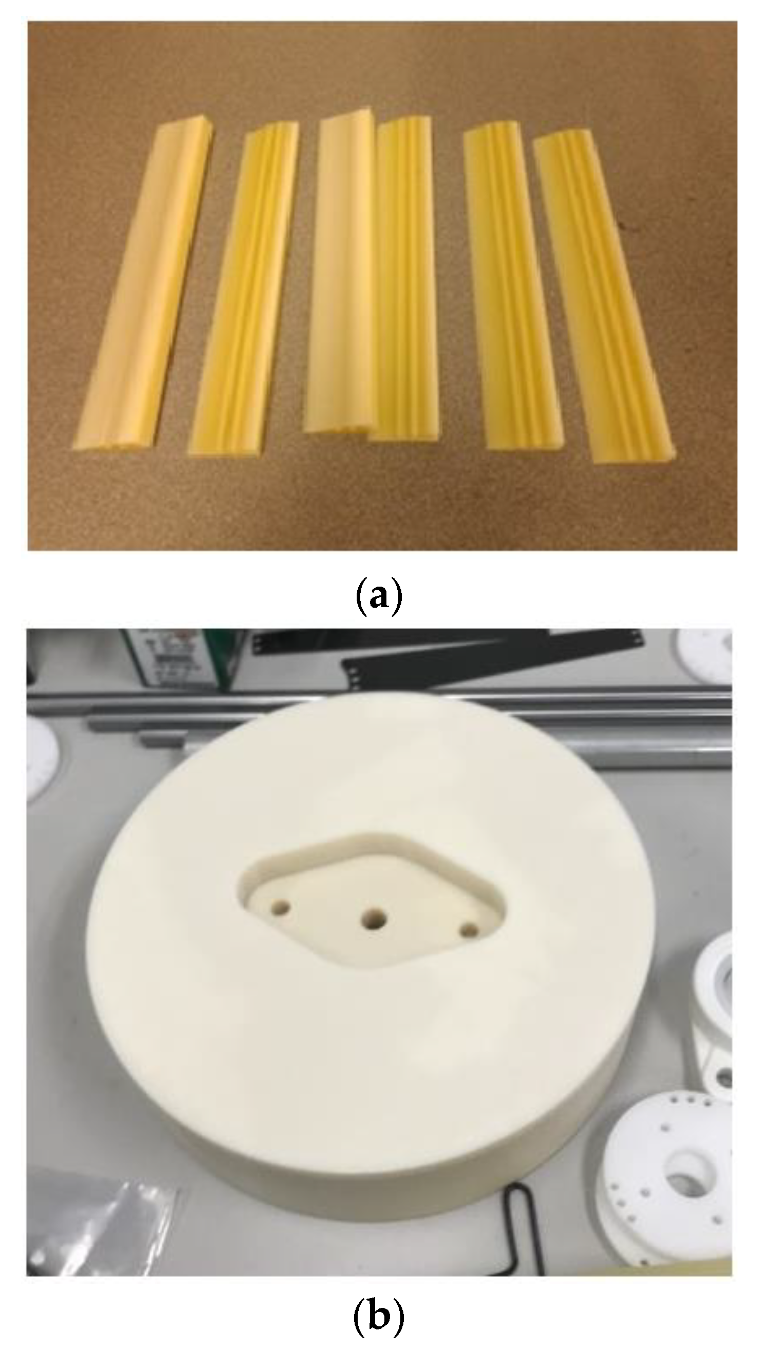
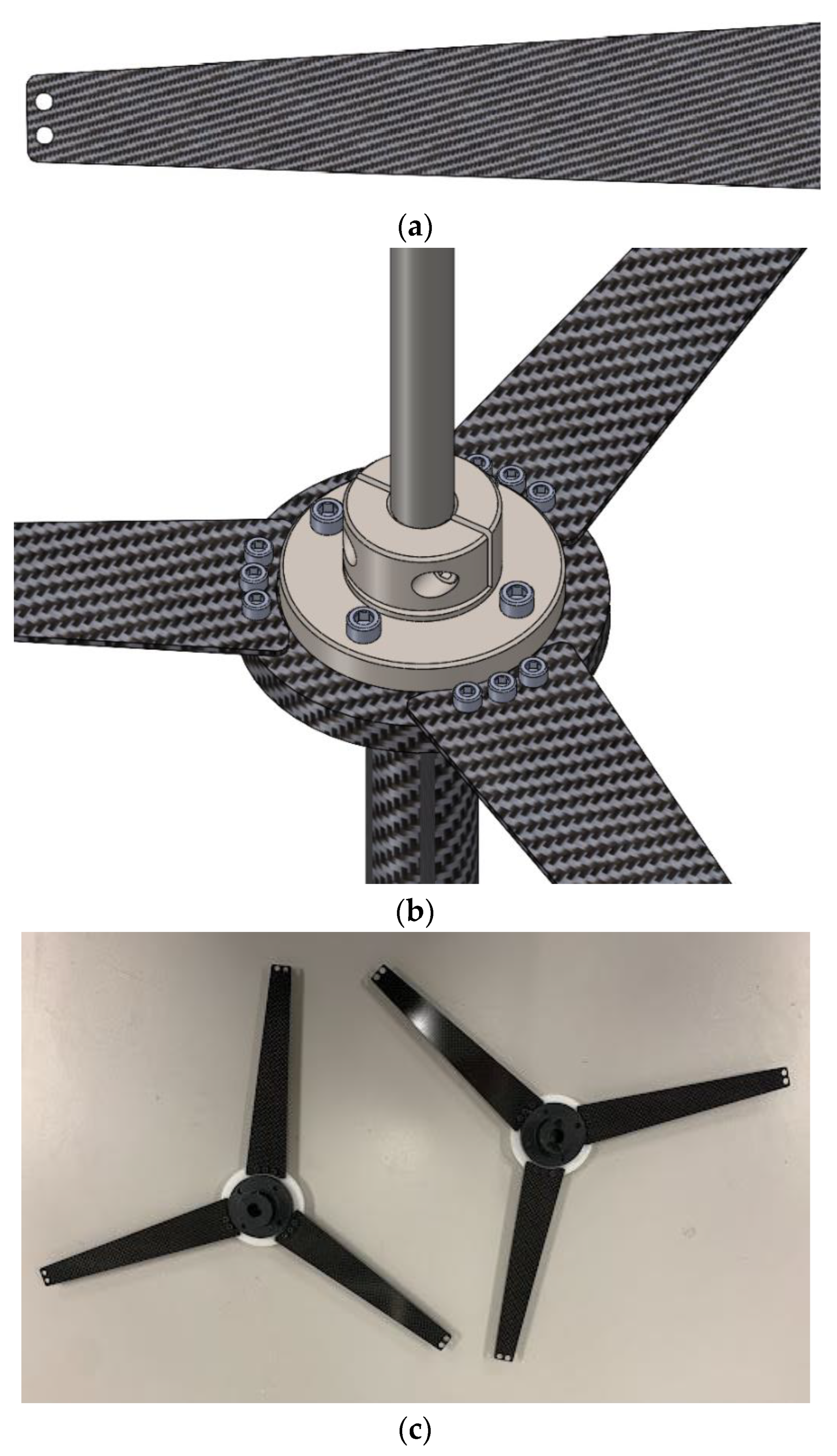
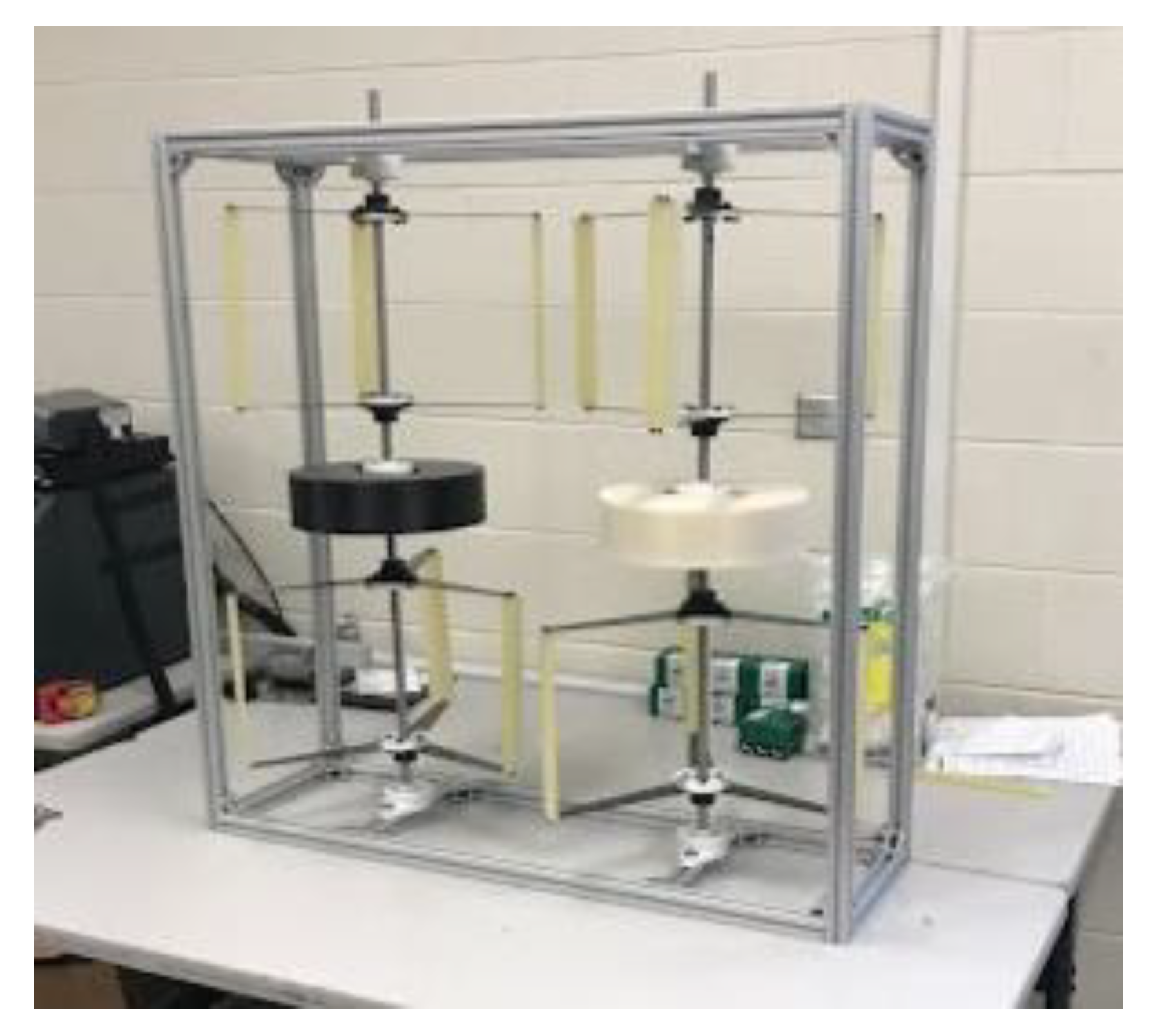
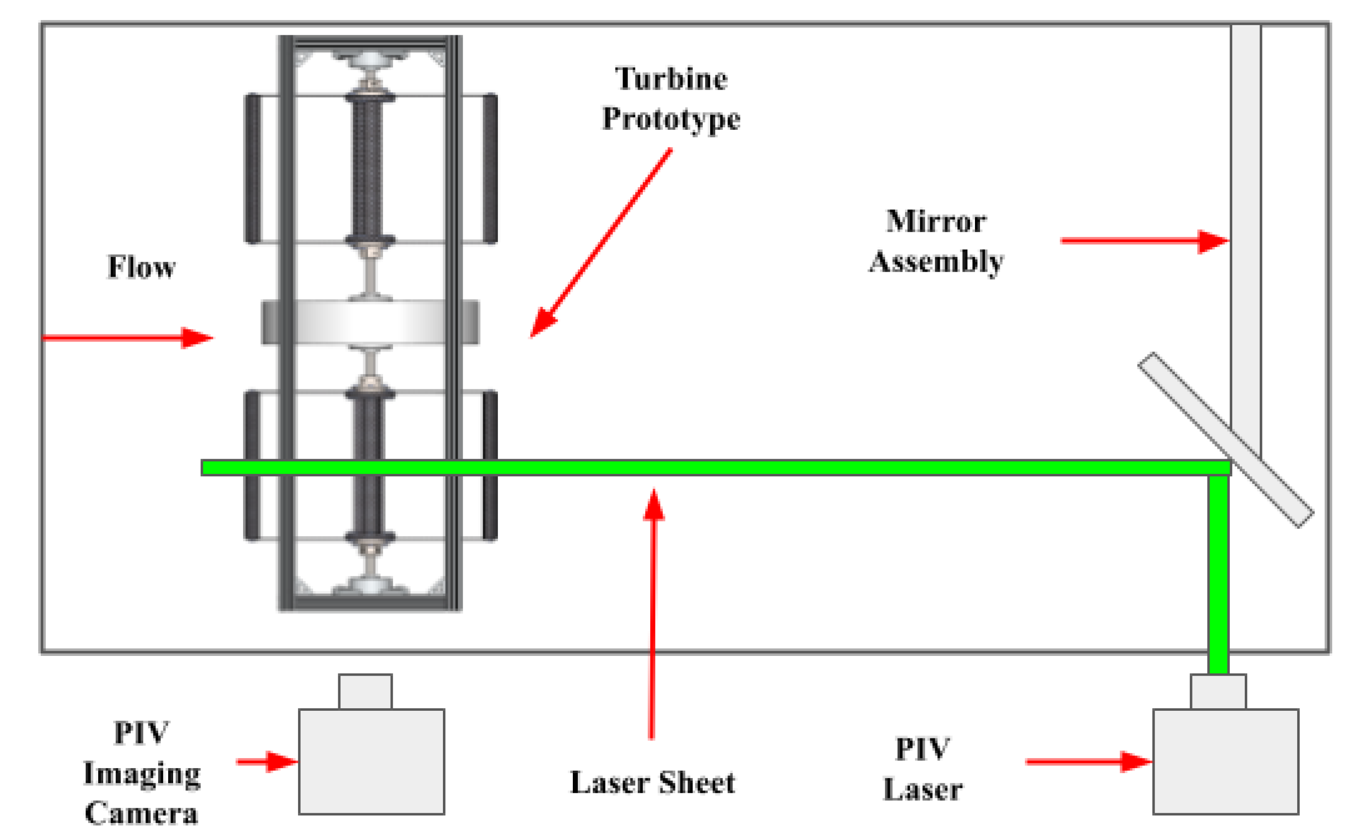
2.1. DD-VADHT Prototype
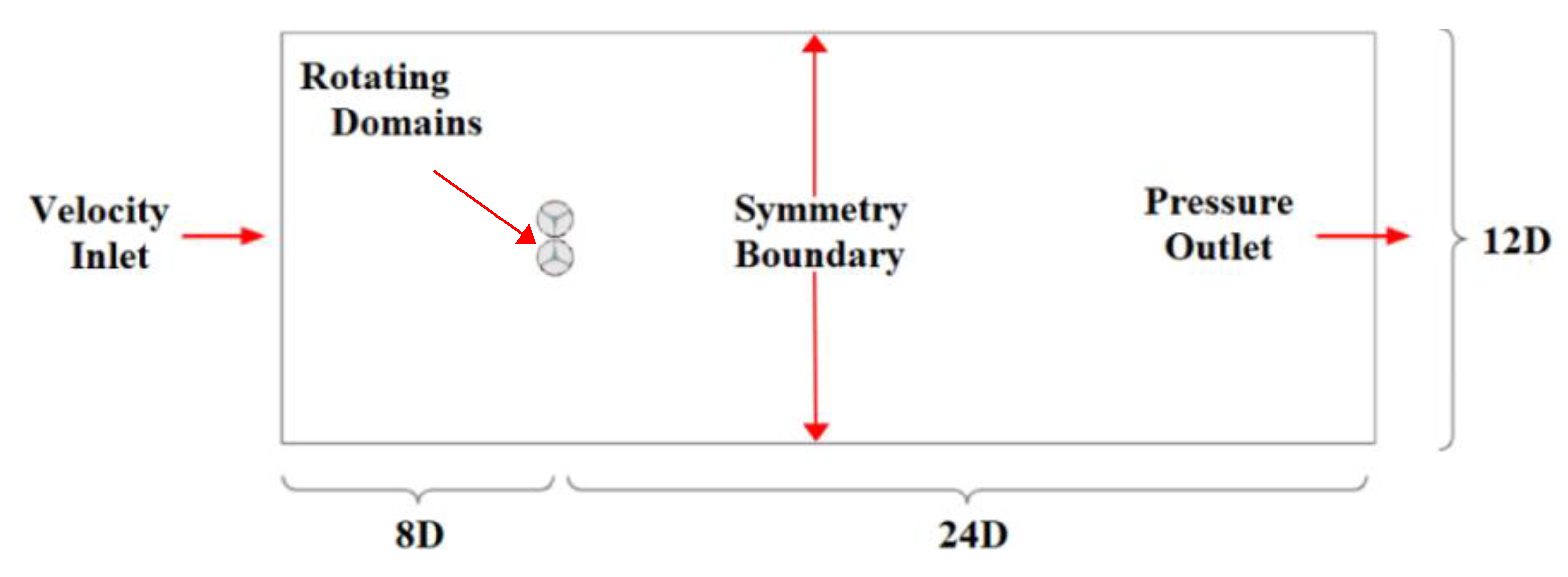
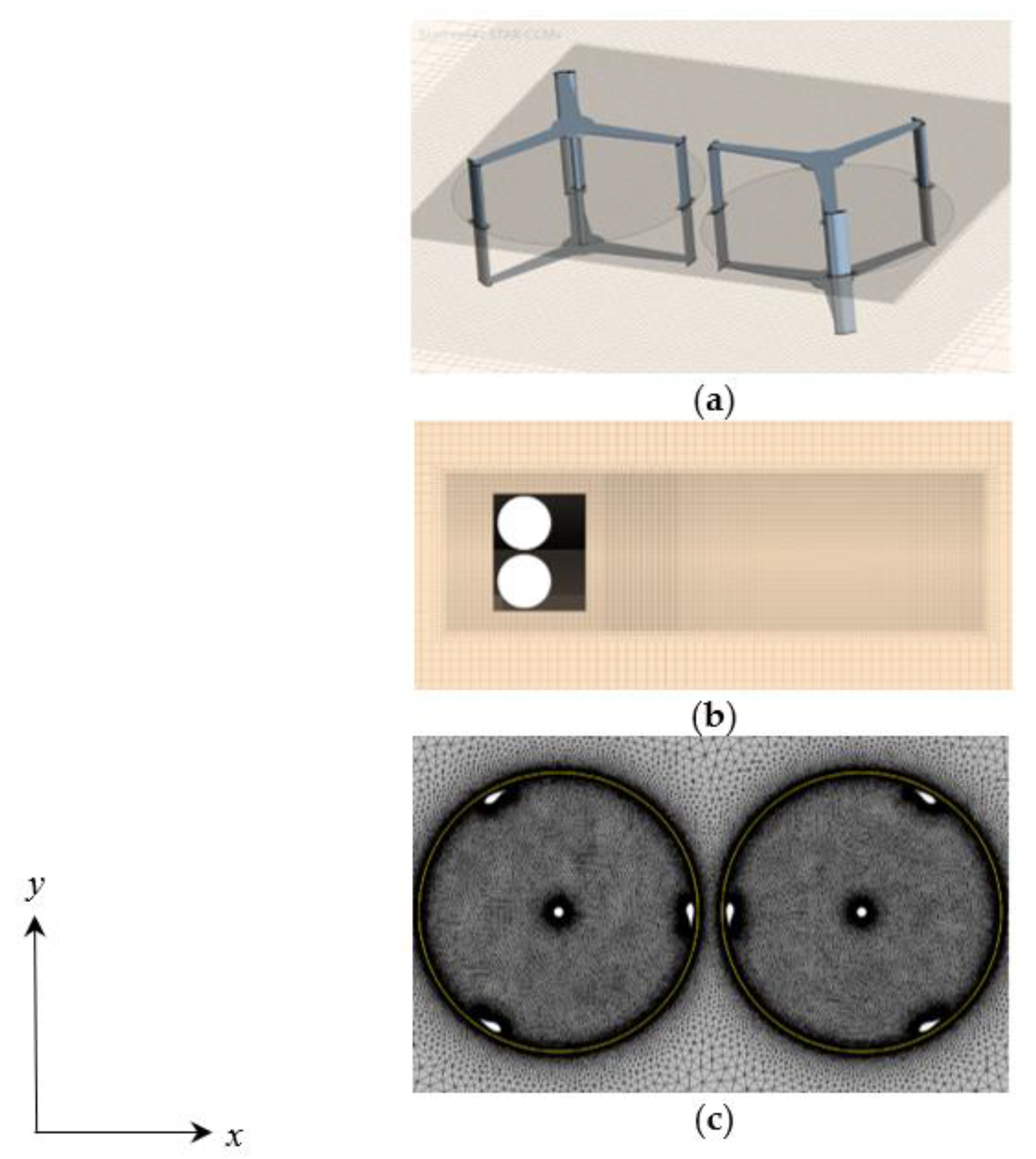
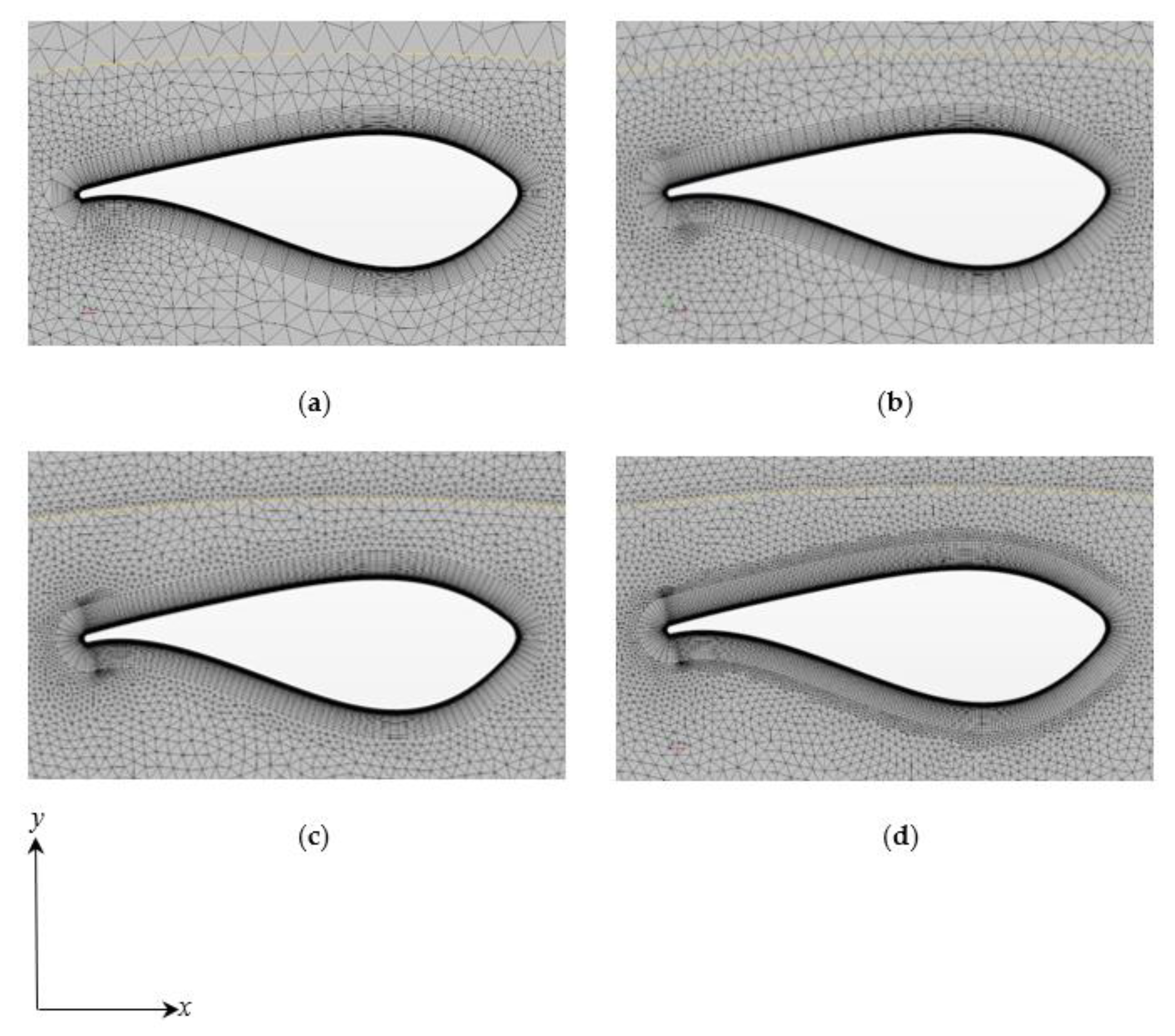
2.2. CFD Modelling and Meshing Methodology
2.3. CFD Flow Modelling Methodology
3. Results
4. Conclusions
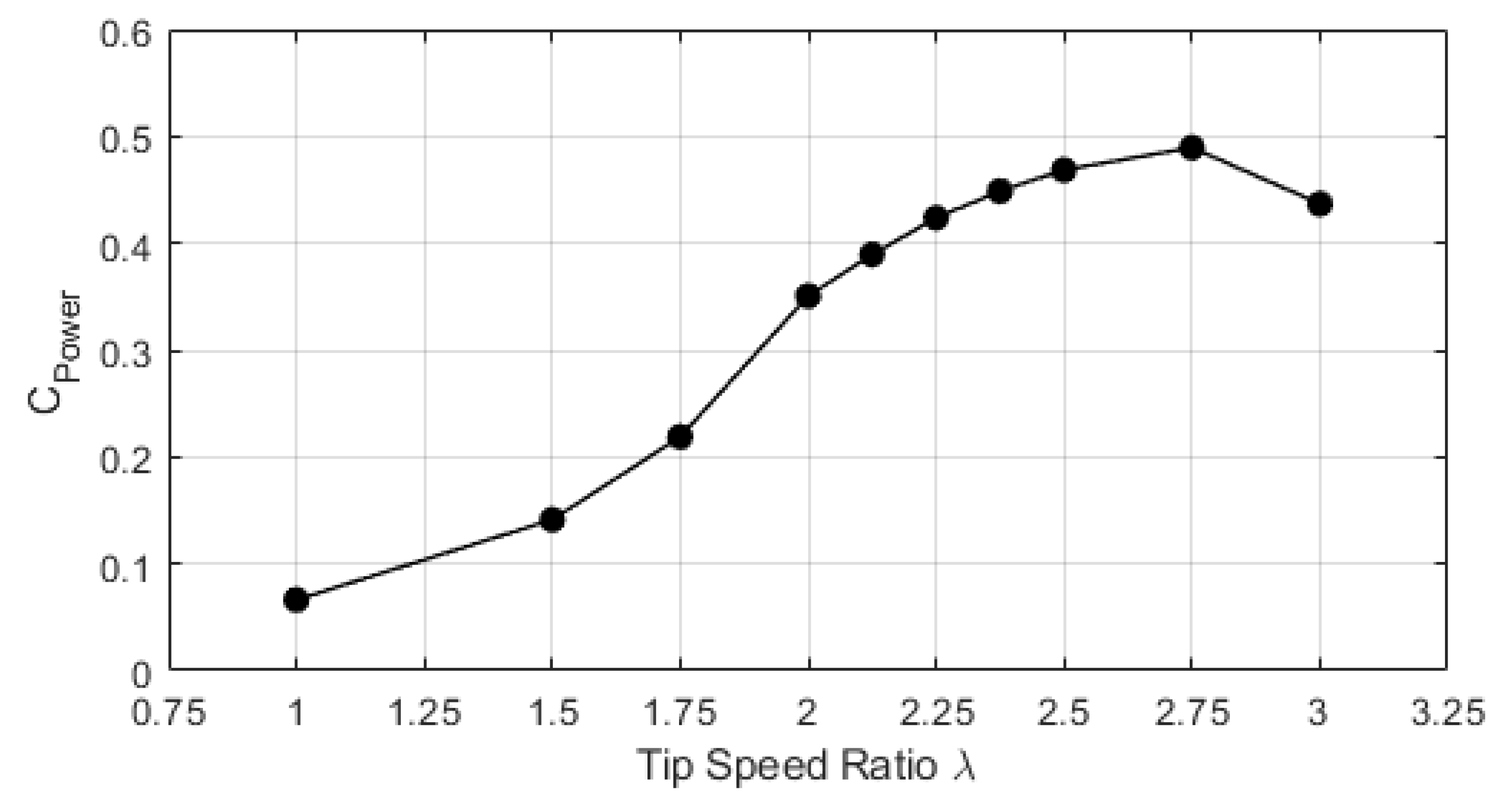
- It appears to be capable of extracting more energy from a double swept area than a single swept area by comparing to previous designs when analyzing ripple effect, torque coefficient, and power coefficient.
- It promises good torque smoothing and possibly good self-starting capabilities, although more work should be done (i.e., CFD, one-dimensional data code analyses and experimental) to verify this.
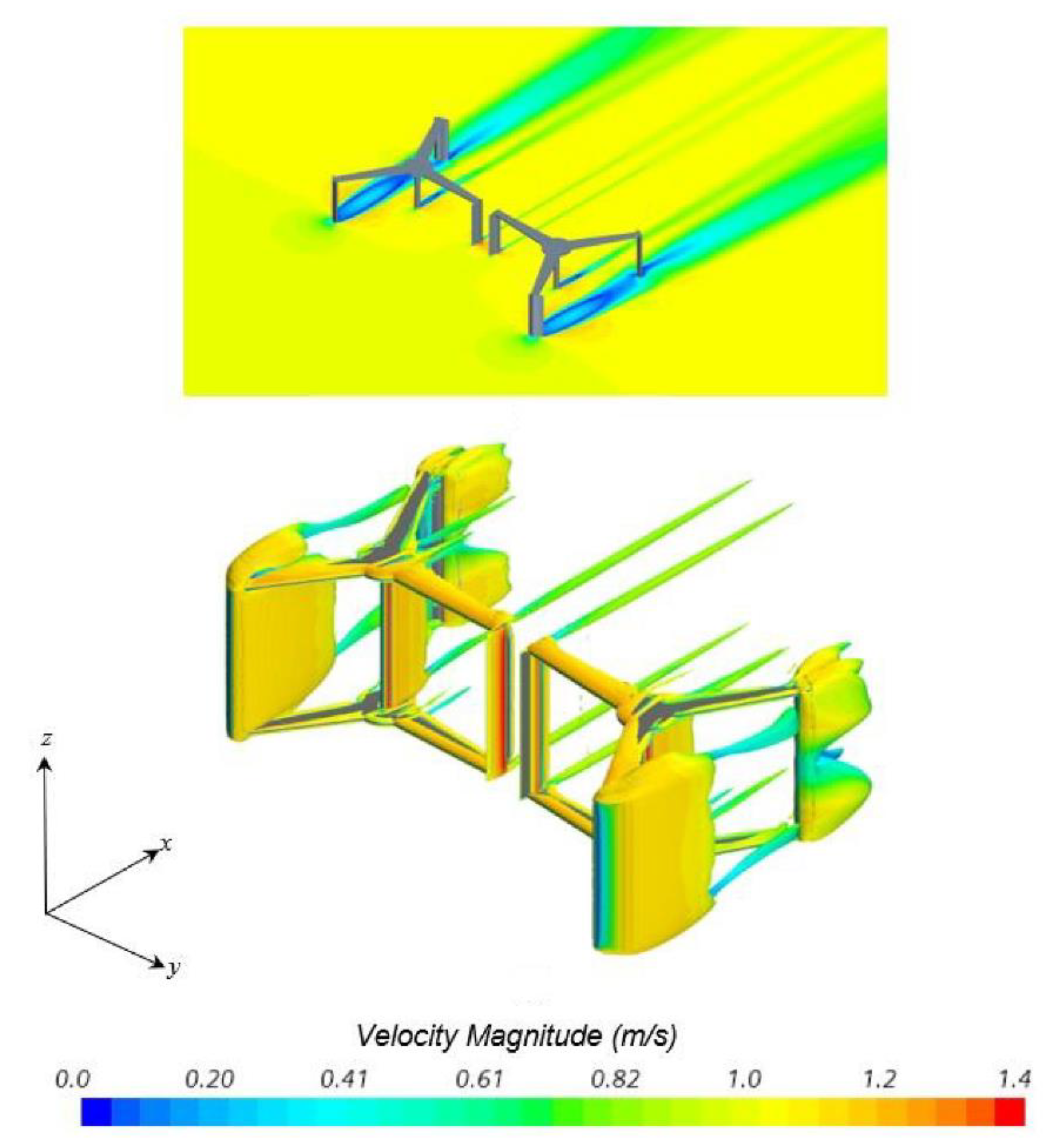
- Additionally, it shows good flow velocity reduction performance for smooth flow transitions between blades and generating sufficient lift.
- A 3-D CFD study should be performed to analyze the vorticity flow pattern behavior between the rotating domains. It is difficult to provide conclusive remarks of vorticity in 2-D simulations as vorticity varies in three dimensions. Better conclusions can be drawn from 3-D simulations regarding vorticity.
- A Large-Eddy Simulation (LES) study will be achieved for analyzing recirculation regions and eddies around curved surfaces and between the rotating domains.
- Analyze multi-blade profiles and lag angles to access performance output using a 2-D simulation over a range of RPMs and inlet flow velocities. A comparison analysis will be helpful in assessing ripple effect for different design configuration and design optimization.
Author Contributions
Funding
Data Availability Statement
Acknowledgments
Conflicts of Interest
Abbreviations
| c | Chord length |
| C1ε | First constant for ε |
| C2ε | Second constant for ε |
| C3ε | Third constant for ε |
| CP | Power coefficient |
| CT | Torque coefficient |
| CTmax | Maximum torque coefficient |
| CTmin | Minimum torque coefficient |
| CTave | Average torque coefficient |
| Cµ | Turbulent eddy viscosity constant |
| Gk | Generation of turbulence kinetic energy due to kinetic energy |
| Gb | Generation of turbulence kinetic energy due to buoyancy |
| H | Turbine height |
| P | Pressure |
| R | Turbine radius |
| Sk | User-defined source term for k |
| Sε | User-defined source terms for ε |
| ui | i-direction velocity |
| uj | j-direction velocity |
| V | Velocity |
| y | Distance to the surface |
| y+ | y plus value |
| YM | Contribution of the fluctuating dilatation in compressible turbulence |
| vt | Eddy viscosity |
| Sij | Strain-rate tensor of the mean field |
| uτ | Friction velocity |
| τ | Reynolds stress tensor |
| τij | Reynolds stress tensor |
| τw | Wall shear stress |
| µ | Dynamic viscosity |
| µt | Turbulent eddy viscosity |
| σk | Turbulent Prandtl number for k |
| σε | Turbulent Prandtl number for ε |
| p | Density |
| ϴ | Azimuth angle |
| λ | Tip speed ratio |
| 2-D | Two-dimensional |
| 3-D | Three-dimensional |
| CFD | Computational fluid dynamics |
| DD-VADHT | Direct-drive vertical axis Darrieus hydrokinetic turbine |
| PIV | Particle image velocimetry |
| RANS | Reynolds-averaged Navier–Stokes |
| TSR | Tip speed Ratio |
References
- Olabi, A.; Abdelkareem, M. Energy storage systems towards 2050. Energy 2020, 219, 119634. [Google Scholar] [CrossRef]
- Han, X.-W.; Zhang, W.-B.; Ma, X.-J.; Zhou, X.; Zhang, Q.; Bao, X.; Guo, Y.-W.; Zhang, L.; Long, J. Review—Technologies and Materials for Water Salinity Gradient Energy Harvesting. J. Electrochem. Soc. 2021, 168, 090505. [Google Scholar] [CrossRef]
- Zhang, Y.X.; Zhao, Y.J.; Li, J.X. Ocean Wave Energy Converters: Technical Principle, Device Realization, and Performance Evaluation. Renew. Sustain. Energy Rev. 2021, 141, 110764. [Google Scholar] [CrossRef]
- González, A.T.; Dunning, P.; Howard, I.; McKee, K.; Wiercigroch, M. Is wave energy untapped potential? Int. J. Mech. Sci. 2021, 205, 106544. [Google Scholar] [CrossRef]
- Ahmed, A.; Azam, A.; Wang, Y.E.; Zhang, Z.; Li, N.; Jia, C.; Mushtaq, R.M.; Rehman, M.; Gueye, T.; Shahid, M.B.; et al. Additively Manufactured Nano-Mechanical Energy Harvesting Systems: Advancements, Potential Applications, Challenges and Future Perspectives. Nano Converg. 2021, 8, 37. [Google Scholar] [CrossRef] [PubMed]
- Xia, C.; Zhu, Y.; Zhou, S.; Peng, H.; Feng, Y.; Zhou, W.; Shi, J.; Zhang, J. Simulation study on transient performance of a marine engine matched with high-pressure SCR system. Int. J. Engine Res. 2022, 98, 107248. [Google Scholar] [CrossRef]
- Ren, L.; Kong, F.P.; Wang, X.F.; Song, Y.; Li, X.; Zhang, F.; Sun, N.; An, H.; Jiang, Z.; Wang, J. Triggering Ambient Polymer-Based Li-O-2 Battery via Photo-Electro-Thermal Energy. Nano Energy 2022, 98, 107248. [Google Scholar] [CrossRef]
- Akinyele, D.; Rayudu, R. Review of Energy Storage Technologies for Sustainable Power Networks. Sustain. Energy Technol. Assess. 2014, 8, 74–91. [Google Scholar] [CrossRef]
- Gunn, K.; Stock-Williams, C. Quantifying the global wave power resource. Renew. Energy 2012, 44, 296–304. [Google Scholar] [CrossRef]
- Dunnett, D.; Wallace, J.S. Electricity generation from wave power in Canada. Renew. Energy 2009, 34, 179–195. [Google Scholar] [CrossRef]
- Khanjanpour, M.; Javadi, A.; Akrami, M. CFD Analyses of Tidal Hydro-turbine (THT) for Utilizing in Sea Water Sealination. In Proceedings of the ISER 209th International Conference, London, UK, 7 July 2019. [Google Scholar]
- Soleimani, K.; Ketabdari, M.J.; Khorasani, F. Feasibility Study on Tidal and Wave Energy Converstion in Iranian Seas. Sustain. Energy Technol. Assess. 2015, 11, 77–86. [Google Scholar]
- Hammons, T.J. Tidal power. Proc. IEEE 1993, 81, 419–433. [Google Scholar] [CrossRef]
- Novo, P.G.; Kyozuka, Y. Tidal stream energy as a potential continuous power producer: A case study for West Japan. Energy Convers. Manag. 2021, 245, 114533. [Google Scholar] [CrossRef]
- Chowdhury, M.S.; Rahman, K.S.; Selvanathan, V.; Nuthammachot, N.; Suklueng, M.; Mostafaeipour, A.; Habib, A.; Akhtaruzzaman; Amin, N.; Techato, K. Current trends and prospects of tidal energy technology. Environ. Dev. Sustain. 2020, 23, 8179–8194. [Google Scholar] [CrossRef]
- Antonio, F.D.O. Wave Energy Utilization: A Review of Technologies. Renew. Sustain. Energy Rev. 2010, 14, 899–918. [Google Scholar]
- Gallego, A.; Side, J.; Baston, E.; Waldman, S.; Bell, M.; James, M.; Davies, I.; O’Hara, R.; Heath, M.; Sabatino, A.; et al. Large Scale Three-Dimensional Modelling for Wave and Tidal Energy Resource and Environmental Impac: Methodologies for Quantifying Acceptable Thresholds for Sustainable Exploitation. Ocean Coast. Manag. 2017, 147, 67–77. [Google Scholar] [CrossRef] [Green Version]
- Träsch, M.; Déporte, A.; Delacroix, S.; Germain, G.; Gaurier, B.; Drevet, J.-B. Wake characterization of an undulating membrane tidal energy converter. Appl. Ocean Res. 2020, 100, 102222. [Google Scholar] [CrossRef]
- Damacharla, P.; Fard, A.J. A Rolling Electrical Generator Design and Model for Ocean Wave Energy Conversion. Inventions 2020, 5, 3. [Google Scholar] [CrossRef] [Green Version]
- Liu, W.; Liu, L.; Wu, H.; Chen, Y.; Zheng, X.; Li, N.; Zhang, Z. Performance analysis and offshore applications of the diffuser augmented tidal turbines. Ships Offshore Struct. 2022, 1–10. [Google Scholar] [CrossRef]
- Mohammed, M. Peformance Investigation of H-rotor Darrieus Turbine with New Airfoil Shapes. Energy 2012, 47, 520–530. [Google Scholar]
- Batten, W.; Bahaj, A.; Molland, A.; Chaplin, J. Experimentally validated numerical method for the hydrodynamic design of horizontal axis tidal turbines. Ocean Eng. 2007, 34, 1013–1020. [Google Scholar] [CrossRef]
- Thiébot, J.; Du Bois, P.B.; Guillou, S. Numerical modeling of the effect of tidal stream turbines on the hydrodynamics and the sediment transport—Application to the Alderney Race (Raz Blanchard), France. Renew. Energy 2015, 75, 356–365. [Google Scholar] [CrossRef]
- Batten, W.; Bahaj, A.; Molland, A.; Chaplin, J. Hydrodynamics of marine current turbines. Renew. Energy 2006, 31, 249–256. [Google Scholar] [CrossRef]
- Polagye, B. Hydrodynamic Effects of Kinetic Power Extraction by In-Stream Tidal Turbines. Ph.D. Thesis, University of Washington, Seattle, WA, USA, 2009. [Google Scholar]
- Cacciali, L.; Battisti, L.; Anna, S.D. Free Surface Double Actuator Disc Theory and Double Multiple Streamtube Model for In-Stream Darrieus Hydrokinetic Turbines. Ocean Eng. 2022, 260, 112017. [Google Scholar] [CrossRef]
- Espina-Valdes, R.; Fernandez-Jimenez, A.; Fernandez-Pacheco, V.M.; Gharib-Yosry, A.; Eduardo, E. Experimental Analysis of the Influence of the Twist Angle of the Blades of Hydrokinetic Darrieus Helical Turbines. Ing. Agua 2022, 26, 205–216. [Google Scholar]
- Kumar, R.; Sarkar, S. Effect of design parameters on the performance of helical Darrieus hydrokinetic turbines. Renew. Sustain. Energy Rev. 2022, 162, 112431. [Google Scholar] [CrossRef]
- Kamal, M.; Saini, R. A review on modifications and performance assessment techniques in cross-flow hydrokinetic system. Sustain. Energy Technol. Assess. 2021, 51, 101933. [Google Scholar] [CrossRef]
- Shaheen, M.; Abdallah, S. Efficient clusters and patterned farms for Darrieus wind turbines. Sustain. Energy Technol. Assess. 2017, 19, 125–135. [Google Scholar] [CrossRef]
- Hau, W. Wind Turbines: Fundamentals, Technologies, Application, Economics; Springer Science & Business Media: Berlin/Heidelberg, Germany, 2013. [Google Scholar]
- Joubert, J.R.; Van Niekerk, J.L.; Reinecke, J.; Meyer, I. Wave Energy Converters (WECs); Centre for Renewable and Sustainable Energy Studies: Cape Town, South Africa, 2013. [Google Scholar]
- Clarke, J.A.; Connor, G.; Grant, A.D.; Johnstone, C.M. Design and testing of a contra-rotating tidal current turbine. Proc. Inst. Mech. Eng. Part A J. Power Energy 2007, 221, 171–179. [Google Scholar] [CrossRef] [Green Version]
- Usui, Y.; Kanemoto, T.; Hiraki, K. Counter-rotating type tidal stream power unit boarded on pillar (performances and flow conditions of tandem propellers). J. Therm. Sci. 2013, 22, 580–585. [Google Scholar] [CrossRef]
- Didane, D.H.; Rosly, N.; Zulkafli, M.F.; Shamsudin, S.S. Performance evaluation of a novel vertical axis wind turbine with coaxial contra-rotating concept. Renew. Energy 2018, 115, 353–361. [Google Scholar] [CrossRef]
- Janon, A.; Boonsuk, T. A Parametric Study of Starting Time Profile for a Novel Direct-Drive Vertical Axis Darrieus Hydroki-netic Turbine with an Axial-Flux Permanent Magnet Generator. In Proceedings of the IEEE 2019 Conference on Power and Energy Systems (ICPES), Perth, Australia, 10–12 December 2019. [Google Scholar]
- Janon, A.; Sangounsak, K.; Sriwannarat, W. Making a case for a Non-standard frequency axial-flux permanent-magnet generator in an ultra-low speed direct-drive hydrokinetic turbine system. AIMS Energy 2020, 8, 156–168. [Google Scholar] [CrossRef]
- Hara, Y.; Horita, N.; Yoshida, S.; Akimoto, H.; Sumi, T. Numerical Analysis of Effects of Arms with Different Cross-Sections on Straight-Bladed Vertical Axis Wind Turbine. Energies 2019, 12, 2106. [Google Scholar] [CrossRef] [Green Version]
- Asbusannuga, H.; Ozkaymak, M. The Effect of Geometry Variants on the Performance on VAWT-Rotor with Incline-Straight Blades. AIP Adv. 2021, 11, 045307. [Google Scholar] [CrossRef]
- Villeneuve, T.; Winckelmans, G.; Dumas, G. Increasing the efficiency of vertical-axis turbines through improved blade support structures. Renew. Energy 2021, 169, 1386–1401. [Google Scholar] [CrossRef]
- Mosbahi, M.; Ayadi, A.; Chouaibi, Y.; Driss, Z.; Tucciarelli, T. Experimental and numerical investigation of the leading edge sweep angle effect on the performance of a delta blades hydrokinetic turbine. Renew. Energy 2020, 162, 1087–1103. [Google Scholar] [CrossRef]
- Vijayan, J.; Renam, B.B. A Brief Study on the Implementation of Helical Cross-Flow Hydrokinetic Turbines for Small Scale Power in the Indian SHP Sector. Int. J. Renew. Energy Dev. 2022, 11, 676–693. [Google Scholar]
- Yagmur, S.; Kose, F. Numerial Evolution of Unsteady Wake Characteristics of H-Type Darrieus Hydrokinetic Trubine for a Hydro Farm Arrangement. Appl. Ocean Res. 2021, 110, 102582. [Google Scholar] [CrossRef]
- Tunio, I.A.; Shah, M.A.; Hussain, T.; Harijan, K.; Mirjat, N.H.; Memon, A.H. Investigation of duct augmented system effect on the overall performance of straight blade Darrieus hydrokinetic turbine. Renew. Energy 2020, 153, 143–154. [Google Scholar] [CrossRef]
- Basumatary, M.; Biswas, A.; Misra, R.D. Experimental verification of improved performance of Savonius turbine with a combined lift and drag based blade profile for ultra-low head river application. Sustain. Energy Technol. Assess. 2021, 44, 100999. [Google Scholar] [CrossRef]
- Mosbahi, M.; Derbel, M.; Lajnef, M.; Mosbahi, B.; Driss, Z.; Aricò, C.; Tucciarelli, T. Performance Study of Twisted Darriues Hydrokinetic Turbine with Novel Blade Design. J. Energy Resour. Technol. Tranaction ASME 2021, 143, 091302. [Google Scholar] [CrossRef]
- Yagmur, S.; Kose, F.; Dogan, S. A study on performance and flow characteristics of single and double H-type Darrieus turbine for a hydro farm application. Energy Convers. Manag. 2021, 245, 114599. [Google Scholar] [CrossRef]
- Arpino, F.; Cortellessa, G.; Scungio, M.; Fresilli, G.; Facci, A.; Frattolillo, A. PIV measurements over a double bladed Darrieus-type vertical axis wind turbine: A validation benchmark. Flow Meas. Instrum. 2021, 82, 102064. [Google Scholar] [CrossRef]
- Keanee, R.D.; Adrian, R.J. Theory of Cross-Correlation Analysis of PIV Images. Appl. Sci. Res. 1992, 49, 191–215. [Google Scholar] [CrossRef]
- Stanislas, M.; Monnier, J.C. Practicle Aspects of Image Recording in Particle Image Velocimetry. Meas. Sci. Technol. 1997, 8, 1417–1426. [Google Scholar] [CrossRef]
- Lazar, E.; DeBlauw, B.; Glumac, N.; Dutton, C.; Elliott, G. A Practical Approach to PIV Uncertainty Analysis. In Proceedings of the 27th AIAA Aerodynamics Measurement and Ground Testing Conference, Chicago, IL, USA, 28 June–1 July 2010. [Google Scholar]
- Raffel, M.; Willer, C.E.; Wereley, S.; Kompenhans, J. Particle Image Velocimetry: A Practical Guide; Springer: Berlin/Heidelberg, Germany, 2007. [Google Scholar]
- Stanley, N.; Ciero, A.; Timms, W.; Hewlin, R.L., Jr. Development of 3-D Printed Optically Clear Rigid Anatomical Vessels for Particle Image Velocimetry Analysis in Cardiovascular Flow. In Proceedings of the ASME 2019 International Mechanical Engineering Congress and Exposition, Volume 7: Fluids Engineering, Salt Lake City, UT, USA, 11–14 November 2019. [Google Scholar] [CrossRef]
- Hewlin, R.L.; Kizito, J.P. Development of an Experimental and Digital Cardiovascular Arterial Model for Transient Hemodynamic and Postural Change Studies: A Preliminary Framework Analysis. Cardiovasc. Eng. Technol. 2018, 9, 1–31. [Google Scholar] [CrossRef]
- Crooks, J.M. Design and Evaluation of a Direct Drive Dual Axis Counter Rotating Hydrokinetic Darrieus Turbine System. Master’s Thesis, University of North Carolinat at Charlotte (UNC-C), Charlotte, NC, USA, 2022. [Google Scholar]
- Hewlin, R.L., Jr.; Smith, E.; Cavalline, T.; Karimoddini, A. Aerodynamic Performance Evaluation of a Skydio UAV via CFD as a Platform for Bridge Girder Inspection: Phase 1 Study. In Proceedings of the ASME 2021 Fluids Engineering Division Summer Meeting, Volume 1: Aerospace Engineering Division Joint Track, Computational Fluid Dynamics, Virtual, 10–12 August 2021. [Google Scholar]
- Maître, T.; Amet, E.; Pellone, C. Modeling of the flow in a Darrieus water turbine: Wall grid refinement analysis and comparison with experiments. Renew. Energy 2013, 51, 497–512. [Google Scholar] [CrossRef]
- Zadeh, S.N.; Komeili, M.; Paraschivoiu, M. Mesh convergence study for 2-D straight-blade vertical axis wind turbine simulations and estimation for 3-D simulations. Trans. Can. Soc. Mech. Eng. 2014, 38, 487–504. [Google Scholar] [CrossRef]
- Sleiti, A.K.; Kapat, J.S. Comparison between EVM and RSM turbulence models in predicting flow and heat transfer in rib-roughened channels. J. Turbul. 2006, 7, N29. [Google Scholar] [CrossRef]
- Allard, M.A. Performance and Wake Analysis of a Darrieus Wind Turbine on the Roof of a Building Using CFD. Master’s Thesis, Concordia University, Montreal, QC, Canada, 2020. [Google Scholar]
- Khan, J.R. Comparison Between Discrete Phase Model and Multiphase Model for Wet Compression. In Proceedings of the ASME Turbo Expo 2013: Turbine Technical Conference and Exposition, Volume 5A: Industrial and Cogeneration, Manufacturing Materials and Metallurgy, Marine; Microturbines, Turbochargers, and Small Turbomachines, San Antonio, TX, USA, 3–7 June 2013. [Google Scholar]
- Alfonsi, G. Reynolds-Averaged Navier–Stokes Equations for Turbulence Modeling. Appl. Mech. Rev. 2009, 62, 040802. [Google Scholar] [CrossRef]
- Kiho, S.; Shiono, M.; Suzuki, K. The power generation from tidal currents by darrieus turbine. Renew. Energy 1996, 9, 1242–1245. [Google Scholar] [CrossRef]
- Niblick, A.L. Experimental and Analytical Study of Helical Cross-Flow Turbines for a Tidal Micropower Generation System. Master’s Thesis, University of Washington, Seattle, WA, USA, 2012. [Google Scholar]
- Hall, T.J. Numerical Simulation of a Cross Flow Maring Hydrokintic Turbine. Master’s Thesis, University of Washington, Seattle, WA, USA, 2012. [Google Scholar]


| Description | Notation | Value |
|---|---|---|
| Chord length | c | 1.3in |
| Turbine radius | R | 8.5in |
| Turbine height | H | 10in |
| Blade profile | - | NACA 0018 |
| Number of blades | N | 3 |
| Tip speed ratio | λ | 2 |
| Step | Description | Parameter |
|---|---|---|
| Camera pixel | CMOS camera pixel specifications | 1920 × 1200 pixels |
| Filter | Band pass filter fitted with the CMOS lens | 532 nm |
| Inlet velocity | Average inlet velocity on the water tunnel | 1 m/s |
| Laser energy | Energy emitted by the laser during acquisition | 700–832 mJ |
| Particle type | Seeding particle diameter and type | 1 µm Glass hollow |
| Frequency | Acquisition frequency of photographs | 15 Hz |
| Time | Time interval between frames | 2 ms |
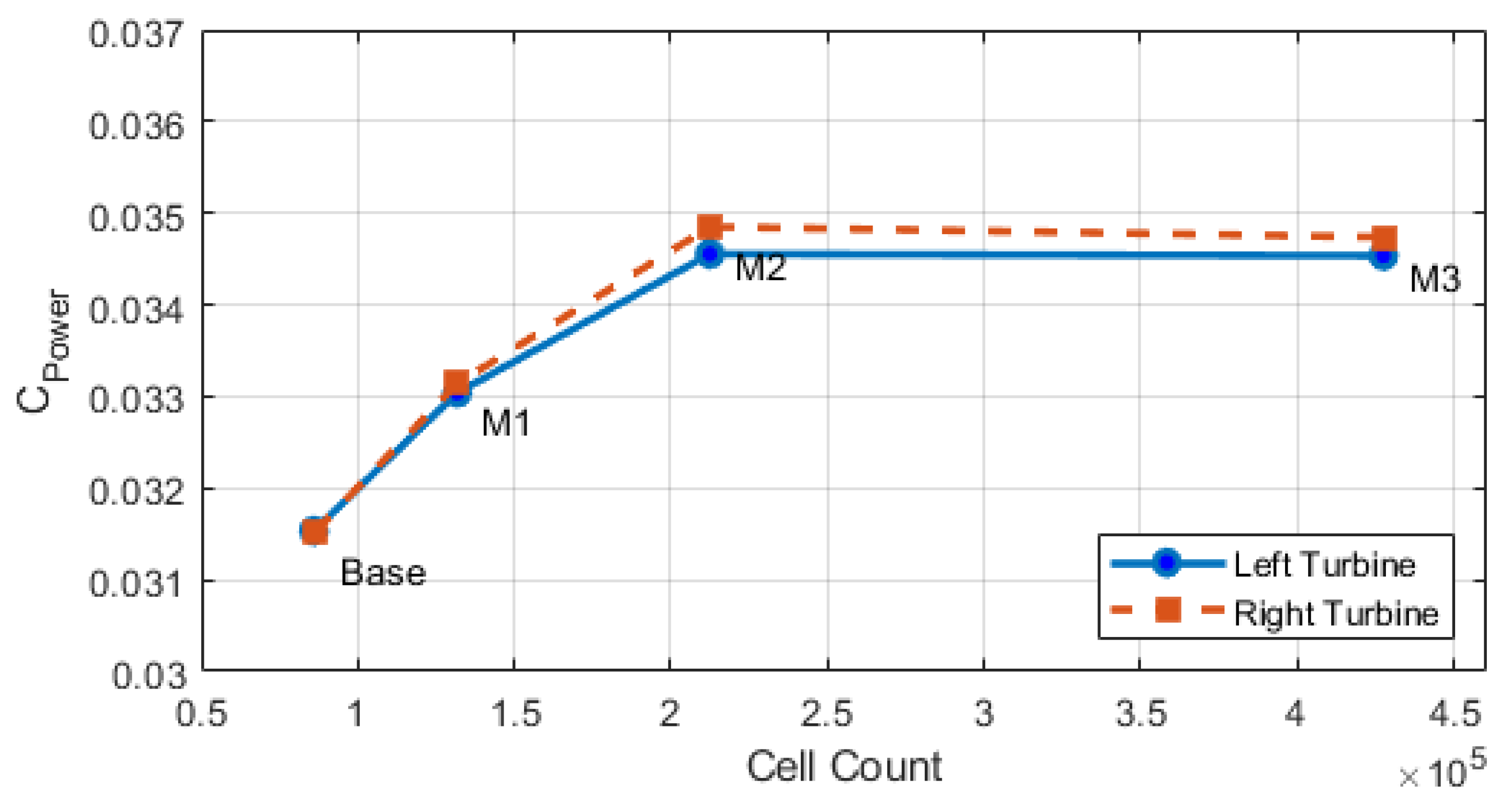
| Mesh | Base Size | Refinement Ratio | Cell Count | Left CP | Left CP |
|---|---|---|---|---|---|
| Base | 10.0in | - | 85,995 | 0.09298 | 0.09291 |
| M1 | 5.0in | 1.53 | 131,750 | 0.09742 | 0.09772 |
| M2 | 2.5in | 1.61 | 212,454 | 0.10189 | 0.10276 |
| M3 | 1.0in | 2.01 | 427,539 | 0.10183 | 0.10243 |
Publisher’s Note: MDPI stays neutral with regard to jurisdictional claims in published maps and institutional affiliations. |
© 2022 by the authors. Licensee MDPI, Basel, Switzerland. This article is an open access article distributed under the terms and conditions of the Creative Commons Attribution (CC BY) license (https://creativecommons.org/licenses/by/4.0/).
Share and Cite
Crooks, J.M.; Hewlin, R.L., Jr.; Williams, W.B. Computational Design Analysis of a Hydrokinetic Horizontal Parallel Stream Direct Drive Counter-Rotating Darrieus Turbine System: A Phase One Design Analysis Study. Energies 2022, 15, 8942. https://doi.org/10.3390/en15238942
Crooks JM, Hewlin RL Jr., Williams WB. Computational Design Analysis of a Hydrokinetic Horizontal Parallel Stream Direct Drive Counter-Rotating Darrieus Turbine System: A Phase One Design Analysis Study. Energies. 2022; 15(23):8942. https://doi.org/10.3390/en15238942
Chicago/Turabian StyleCrooks, John M., Rodward L. Hewlin, Jr., and Wesley B. Williams. 2022. "Computational Design Analysis of a Hydrokinetic Horizontal Parallel Stream Direct Drive Counter-Rotating Darrieus Turbine System: A Phase One Design Analysis Study" Energies 15, no. 23: 8942. https://doi.org/10.3390/en15238942