
Optimum Parallel Processing Schemes to Improve the Computation Speed for Renewable Energy Allocation and Sizing Problems

1
Department of Electrical Engineering, Istanbul Technical University, 34467 Istanbul, Turkey
2
Department of Electrical Engineering, Mathematics and Computer Science, University of Twente, 7522 NB Enschede, The Netherlands
3
Department of Electrical and Electronics Engineering, Marmara University, 34722 Istanbul, Turkey
*
Author to whom correspondence should be addressed.
Energies 2022, 15(24), 9301; https://doi.org/10.3390/en15249301
Submission received: 4 November 2022
/
Revised: 2 December 2022
/
Accepted: 6 December 2022
/
Published: 8 December 2022
(This article belongs to the Special Issue Modeling and Analysis of Active Distribution Networks and Smart Grids)
Abstract
:The optimum penetration of distributed generations into the distribution grid provides several technical and economic benefits. However, the computational time required to solve the constrained optimization problems increases with the increasing network scale and may be too long for online implementations. This paper presents a parallel solution of a multi-objective distributed generation (DG) allocation and sizing problem to handle a large number of computations. The aim is to find the optimum number of processors in addition to energy loss and DG cost minimization. The proposed formulation is applied to a 33-bus test system, and the results are compared with themselves and with the base case operating conditions using the optimal values and three popular multi-objective optimization metrics. The results show that comparable solutions with high-efficiency values can be obtained up to a certain number of processors.
1. Introduction
1.1. Background
Optimization tools are used in various studies to make the best decisions possible in swarm-based problems [1,2,3]. Researchers have been considering more details of the methods and datasets in order to obtain more reliable and fast solutions for their optimization problems. The number of calculations and computational time increase with the increasing scale of the network and the number and type of objectives. In some cases, simulations can take several days or even weeks to complete the process. The deployment of parallel computing to handle a large number of computations is the primary focus of this study. Moreover, we aim to analyze the relationship between the accuracy and the speed of the performed parallel computation since parallel computing may converge to different values than serial computing. In this regard, the results for both cases are compared, and the accuracy of parallel computing is evaluated comparatively.
DGs have been penetrating into the distribution network for energy loss minimization [4,5,6], voltage profile improvement [7,8,9], peak clipping, cost minimization [10], and similar purposes through constrained optimization formulations. Therefore, the optimal DG siting and sizing problem involves solving algebraic or differential equations concerning the consolidation of high- and low-energy consumption points in the power grid. The number of calculations is also related to consumer behavior and the number of alternative locations [11]. Most of the past studies have concentrated on the formulation of DG siting and sizing problems, while decreasing the computational time was relatively discarded. However, the computational time required for reliable solutions for the increasing number of inputs and objective functions is getting more important day by day, especially for operational problems involving real-time solutions.
This study is therefore devoted to decreasing the computational time of optimal DG planning problems. In this regard, we investigated the most efficient parallel computing scheme that reduces the computational time without scarifying the accuracy of the serial configurations. The related formulation is tested in known power distribution test systems.
1.2. Literature Review
Many formulations have been proposed for the siting and sizing of DGs, some focusing on the single-objective problem, others on multi-objectives aiming to reduce active losses [12], improve the voltage profiles [13], improve the reliability indices of the distribution network (DN) [14], minimize the emission rate [15], provide better load distribution by peak clipping [16], and reduce the operation cost of micro-grids without bringing discomfort to the users [17]. Among several alternatives, photovoltaics (PVs) and wind turbines (WTs) are the two most-common DG units that can be placed close to the load centers. In [11], a nonlinear single- or multi-objective cost function was minimized in order to achieve optimal DG allocation and sizing, which was developed in accordance with the utilities’ interests and concerns. Then, optimization equations were solved using either analytical methods or heuristic approaches, depending on the problem types and desired computational speed. Due to the application ease of their derivative-free solution procedures for the formulations comprising the use of both the integer and the real control variables, heuristic approaches are often preferred.
The optimum sizing and siting of a single DG to minimize the daily energy losses and voltage violations in a DN was achieved by employing the meta-heuristic cuckoo search algorithm [18]. Then, the resulting daily percentage energy losses were decreased from 3.46% to 0.92% and 3.75% to 1.01% without any voltage magnitude violations for the summer and winter seasons, respectively. Sultana et al. used the grey wolf optimizer (GWO) for multi-DG allocation and sizing in a distribution system to minimize the reactive power losses and improve the voltage profiles [19]. Another study used an analytical method for expansion planning of the Addis North distribution network, considering the integration of the optimal sizes of distributed generations for the projected demand growths [20]. The active and reactive power losses were minimized by 21.285% and 19.633%, respectively, and the voltage profiles were improved by 8.78%. A multi-objective ant lion optimization (ALO) algorithm was modified to determine the near-optimal numbers, sizes, locations, and types of the DG units for the objectives of voltage profile improvement and installation cost minimization [21]. The resulting optimal values were then tested with the extreme monthly distributions to identify the impacts of load and generation volatilities on the voltage profiles. The enhanced multi-objective harmony search optimization algorithm reduced the power losses and improved the voltage profiles [22]. Another paper used the same heuristic algorithm to determine the optimal state of switching devices (open or closed) in a given distribution network, aiming to minimize active power losses [23].
The ALO algorithm and its multi-objective variation (MOALO) are becoming more well-known in recent times. It was used to address smart grid issues such as voltage profile improvement, cost optimization of distributed generation, and power loss reduction in [24,25]. In [26], the authors found optimal distributed energy resource (DER) size configurations that aim to minimize DER losses. The MOALO algorithm was used in this work to determine the Pareto-front-optimal solutions to minimize installation costs and optimize voltage profiles.
There are several parallel computing applications in the power systems area. In [27], the authors solved the optimal switching problem by parallel processing of mixed-integer linear programming. The authors of [28] solved the reactive power optimization problem by using an adaptive differential evolution method. Several heuristic algorithms were utilized for parallel computing in solving bidding problems in local energy markets in [29]. A parallel particle swarm optimization was used in [30] to maximize the profits of the industrial customers that provide operational services to the power grid. The economic dispatch problem was solved using a parallel bat algorithm in [31]. An optimal distributed reactive power supply was formulated and solved by using a parallel harmony search algorithm in [32].
In most of the studies related to parallel computing, the main aim was to improve communication and cooperation among processors to increase computational speed and efficiency [33,34,35,36,37,38]. In [33], the authors tried to explain how to achieve multi-processor operations with excellent efficiency by making better use of multiple processors. Three techniques, namely the parallel island model, parallel evaluation of a population, and parallel evaluation of a single solution were used. This paper will utilize the second method, which is a variation of the master/slave method.
Speedup and efficiency are the most popular parameters used to evaluate the computational speed in parallel processing. The speedup of an n-processor computation is the ratio of the time required to solve a problem with a single processor to the time required to solve the problem with n processors. It is obvious that an ideal system with n-processors has a speedup equal to n. However, this is not the case in practice since each processor spends some time on communication and cannot use 100% of its time for computation. Therefore, efficiency is used to measure the percentage of time that a processor uses for the computation task. In other words, the speedup compares how many times faster a problem can be solved as a function of the number of parallel units, and efficiency measures how much of that benefit is obtained per contributing processor unit [39].
1.3. Contribution
With the advancement of technology and increase in the size of the network, it is necessary to address more complex issues in order to make the best decisions among several alternatives. This issue motivated us to gather a great deal of information in the relevant field, which increases the number of calculations required to arrive at the best decision. However, one of the most-significant considerations for researchers is the calculation time. The associated literature for such research reveals few investigations into time consumption, despite the fact that it must be included. In this regard, the computational time is handled as an additional objective in this paper, along with the other network objectives.
The following summarizes the major contributions of the study:
- A parallel computation approach based on the master/slave method is applied to the optimal allocation and sizing of DG units in a DN, considering minimizing energy losses and DG costs.
- The impacts of the number of parallel processors on the optimal control parameters, objective functions, and dependability of the method are determined.
- The range of the optimal number of parallel processors providing better speedup and efficiency is determined.
- Optimum solutions for the different number of processors are discussed with respect to three multi-objective optimization performance criteria.
The structure of the paper is as follows. The proposed problem’s formulation is covered in Section 2. The implementation of the optimization algorithm and its paralleling solution are discussed in Section 3. The test systems are detailed in Section 4, and the results are analyzed in Section 5. Conclusions are summarized in Section 6.
2. Problem Formulation
2.1. Objectives
This article aims to decrease the computational time of a multi-objective optimization problem to minimize active energy losses and annual DG costs. The mathematical formulation of the optimization problem can be stated as follows:
where and are the two objective functions and and are the location and the size of the intended DGs, respectively. and are the equality and inequality constraint of the state variables , respectively. The details will be discussed in Section 2.2.
2.1.1. Active Energy Losses
The first objective function of the optimization problem is the energy losses along a specified period. Mathematically, it can be expressed as
where represents the entire optimization time frame in hours, corresponds to the number of buses in the feeder, and is the resistance of the line connecting buses j and k. At hour-i, is the line current between buses j and k. The limit violation of the dependent variables (here, bus voltage magnitudes) is often embedded in the objective function using penalty factors [40]. In this regard, the augmented objective function is expressed as follows:
where C is the constant that balances the penalty term and the main OF and P is the penalty factor expressed below.
The voltage magnitude of at is denoted by . Because of the high resistance (R) over the reactance (X) ratios, unbalanced characteristics of the distributed load, radial configuration of the feeder, and dispersed generation in the distribution lines [41], we used the forward–backward sweep (FBS) technique to solve the power flow equations.
2.1.2. Annual DG Costs
The second objective of the process is to reduce the annual investment and operating costs of PV and WT units. PV and WT expenses are calculated on an annual basis and include installation, operation, and maintenance costs. Notably, regardless of their size, DG units are assumed to have the same unit costs and estimated lifespan. The annual DG cost formulation is given below:
where and represent the overall annual cost of PV and WT units. These costs are proportional to the DG sizes (power).
where refers to the marginal unit setup cost in USD/kW, whereas denotes the units’ annual marginal operational and maintenance costs in USD/kW−yr. The unit’s anticipated lifetime in years is denoted by , and the unit size is denoted by S; and indicate the total number of DG units determined by the optimization procedure. Finally, denotes the capacity recovery factor of a DER unit with a lifetime of years and an interest rate of r.
2.2. Problem Constraints
2.2.1. Equality Constraints (Power Balance Equations)
The equality constraints of the optimization are the nodal power balance equations at each time bin:
where P and Q denote the active and reactive powers, respectively. The subscripts MG, PV, WT, load, and losses signify the main grid, PV unit, WT unit, bus load, and feeder losses, respectively. The subscript i denotes the time bin at which the balance is supplied.
2.2.2. Limits of Main Grid Supply
Limits of main grid supply are stated below:
where and represent the maximum active and reactive power that the main grid can supply at , respectively. Note that these limits rely on the main grid generation capacity at and corresponding load level of the distribution grid [21].
2.2.3. Limits of WT and PV Generation
The active power generation of the WT and PV units was restricted to 1 MW, considering the incentives provided for the distributed generation units having 1 MW and lower capacity in Turkey. On the other hand, the lower limit for DG units was set to 500 kW to enable a fixed unit size cost for all DG units to be more realistic.
3. Implementation of Particle Swarm Optimization Algorithm and Parallel Processing
3.1. Particle Swarm Optimization Algorithm
Particle swarm optimization (PSO) is a nature-inspired meta-heuristic method that mimics the social behavior of birds and has grown in popularity for solving multi-objective optimization problems. The details of the method can be found in [42,43]. The most-common abbreviated description of the PSO algorithm, expressed in this manner, is as follows: In a D-dimensional search space, each particle represents a possible solution to the optimized problem, and it can memorize both the ideal location of the swarm and its own position. As each new generation of particles is born, various particle information is gathered and used to compute the new location of the new generation of particles. The particles go around the multi-dimensional search space, gradually changing states until they find an optimal state or until calculation limitations are reached. A unique relationship is established via the objective functions, which act as a connecting link between the aspects of the objective space. This method has had a considerable amount of empirical data to support it.
3.2. Overview of Multi-Objective Optimization Process
An expression for an n-dimensional multi-objective optimization model is formulated as
where is a control and state variable vector, is the ith objective function, and and are the inequality and equality constraints, respectively. The Pareto optimality idea is applied in multi-objective optimization problems to generate non-dominated solutions, which are also known as Pareto-optimal solutions [44]. This approach enables the flexibility of selecting the best solution from a set of near-Pareto-optimal solutions based on problem-specific needs.
3.3. Parallel Processing of Multi-Objective PSO Algorithm
This study uses the master/slave communication policy of the processors inherited from [33]. The method uses a master processor (MP) and a predetermined number of migration points (MPs). Note that the number of iterations is constant for all slave processors, and at each MP, the slave processors send their results to the MP [33]. When the final MP is reached, the MP publishes the final proposed solution as the final solution. The flow chart of the parallel processing depicted in Figure 1 explains the process visually. Note that the domination percentage (DP) index is used to determine the non-dominated solutions found by slave processors. The details of the DP index are explained in Section 5.2.1.
As can be seen from the figure, after the computation procedure starts in the master processor, a variable named as iterations per processor (IPP) is created. This variable is responsible for determining the iterations performed on each processor. After a processor obtains this information, it locally initializes its swarm by using randomly created values of the variables (locations and sizes of the DGs) in the allowed ranges. Then, the objective function is evaluated for all the swarm members, and the objective function values are calculated. The best-ever position for any particle and the best position in the current swarm are stored as and . Then, the velocity and the position values are updated according to the given equations, in each iteration:
Note that x and v represent the position of the particle and its velocity, respectively. The two coefficients and are generally taken as 2. Another coefficient w is called the inertia factor, which is generally taken as a value between 0.4 and 1.4. The i and k values are used for representing an individual particle in a swarm and the iteration number, respectively.
Then, the non-dominated particles need to be found. There are three possibilities for any two particles ( and ); may dominate ; may dominate ; neither nor dominate the other one based on the Pareto dominance definition given below.
Definition 1.
Pareto dominance: The particle dominates with m objective values, if:
The next step updates the set of non-dominated solutions by using the non-dominated particles. The method applies the crowding distance, which is a parameter for calculating the distance between the non-dominated set of particles to control the number of non-dominated particles to update non-dominated particles. It can allow the new non-dominated particles to be added to a set of non-dominated particles either by updating or removing some particles when the set becomes full. This process is briefly explained as follows:
- The new particle is not added to the archive set if at least one non-dominated particle dominates it.
- An additional particle is added to the set if it dominates any non-dominated particle, and the corresponding particle is thus removed.
- This new solution is added to the set if the new particle does not dominate any non-dominated particles in the set.
- In the case that the set of non-dominated particles reaches its capacity when a new particle needs to be added, the grid mechanism is used to reorganize the objective domain, and the most-crowded segment removes a particle from the set. Please refer to [40] for more details.
The local algorithm in a processor then checks if the migration point is reached. If this is not the case, it continues the process of updating the operation of the velocity and position of the particles. If the migration point is reached, it sends its Pareto solutions to the master processor. If the last migration point is reached, it again sends the Pareto solutions to the master processor.
The master processor is responsible for receiving all Pareto fronts sent by all processors, then it sorts them according to the DP evaluation [9] and sends them back to all processors. If all processors reach their last migration point, then it again receives all the Pareto solutions and lists them as the final solutions.
Although the number of MPs can be adjusted to any value, the accuracy of the computations is heavily reliant on this parameter. It is self-evident that selecting a small MP value leads to an unreliable solution, while selecting a large MP value leads to low computing efficiency. This is discussed in detail in [45], where the ideal number of processors and the MPs were determined as 20 and 50, respectively. We will utilize the same MP value for parallel execution in this study.
4. Test Systems
The proposed methodology was applied to the 33-bus radial distribution test system given in Figure 2 [46]. Note that the base case total load of the system is 5084.26 kW and 2547.32 kVAR, respectively. All the feeder buses are considered to be applicable for DG allocation except the main generator (grid) bus, and more than one DG is not allowed to be allocated in the same bus. The scaled daily load curve is illustrated in Figure 3a. Note that the figure comprises average values for three consecutive days (72 h), representing the summer, fall/spring, and winter seasons. The load patterns were taken from the Turkish distribution grid, and the details can be found in [47].
The average daily outputs of PV and WT units are depicted in Figure 3b and Figure 3c, respectively. They are the averages of the seasonal loads of one year of data from a specific region in Turkey, where the average capacity factors are 35% and 34% for the WT and PV units, respectively. The details can be found in [47]. Note that all the outputs are scaled to their rated values, and the same output characteristics are used for similar types of PV and WT units in the feeder since the feeder lengths are short enough so that the units will experience the same meteorological conditions.
On the other hand, the DG outputs were limited to 1 MW, considering the side-specific financial incentives provided for the DG units having 1 MW or less capacity in Turkey. Moreover, the minimum DG size was set to 50 kW so that a fixed unit size cost for all DG units will be more meaningful. Finally, we limited the maximum number of DG units installed in the system to 8 regardless of their types, considering the practical availability conditions in real distribution networks in Turkey.
5. Results and Discussion
Six different parallel simulation scenarios were tested for the same network and DG configurations. Each scenario tries to solve the mentioned constrained optimization problem using a different number of processors, 1, 2, 6, 10, 15, and 20. The number of MPs was set to 50 for all scenarios, ensuring the best-possible optimal communication between the processors. The processor model was selected as an Intel (R) Xeon (R) CPU E5-2680 v4 @ 2.40 GHz. Please refer to [48] for the processor details. We used Matlab’s parallel computing toolbox for performing parallel simulations [49].
The specific functionalities to send, receive, and broadcast the data that allows message-passing-type communications were utilized. We set the maximum number of iterations and the maximum number of execution of the code to 10,000 and 100, respectively. Although the simulation in [45] indicated that 700 iterations are sufficient for such optimization issues, our study attempted to propose a more reliable solution by increasing both the number of iterations and the number of executions. The 30 search agents were assigned to the optimizer alongside a repository size of 200.
The simulation period was chosen as 72 h (three days), where each day was considered for one season. The constant C in Equation (3) was set to 100, which was found to be the best value balancing the losses and voltage violations for the test system’s load data. The relevant DG parameters used in the simulations are illustrated in Table 1.
Using the simulation times as a starting point, the results were compared to find the best number of processors based on the speedup and efficiency indices. Then, the best Pareto solutions found by the simulations were determined, and the optimality of the solutions was tested based on the DP, hypervolume (HV) index, and spacing index [40].
5.1. Speedup and Efficiency
The computational time statistics are illustrated in Table 2. The average computational times (ACTs) are also depicted in Figure 4. As expected, the ACT of a single processor case, 4886 seconds, decreases with the increasing number of processors. The resulting ACTs are 47.0%, 15.2%, 9.2%, 6.9%, and 5.9% of the base case serial ACT for 2, 6, 10, 15, and 20 processors, respectively. On the other hand, the relative standard deviation (standard deviation/ACT) of the computational time is 8.5% for the serial case. It increases with the number of processors and becomes 22.8% for the 20-processor case. A Similar behavior is also valid for the relative solution range ([Max. value-Min.value]/ACT) of the computational times. These increasing relative standard deviations and relative solution ranges with the rising number of processors indicate an increase in the dispersion of the solutions. This can be interpreted as the increasing number of processors decreasing the dependability of the solutions, which in turn brings an upper limit on the number of processors in practical implementations.
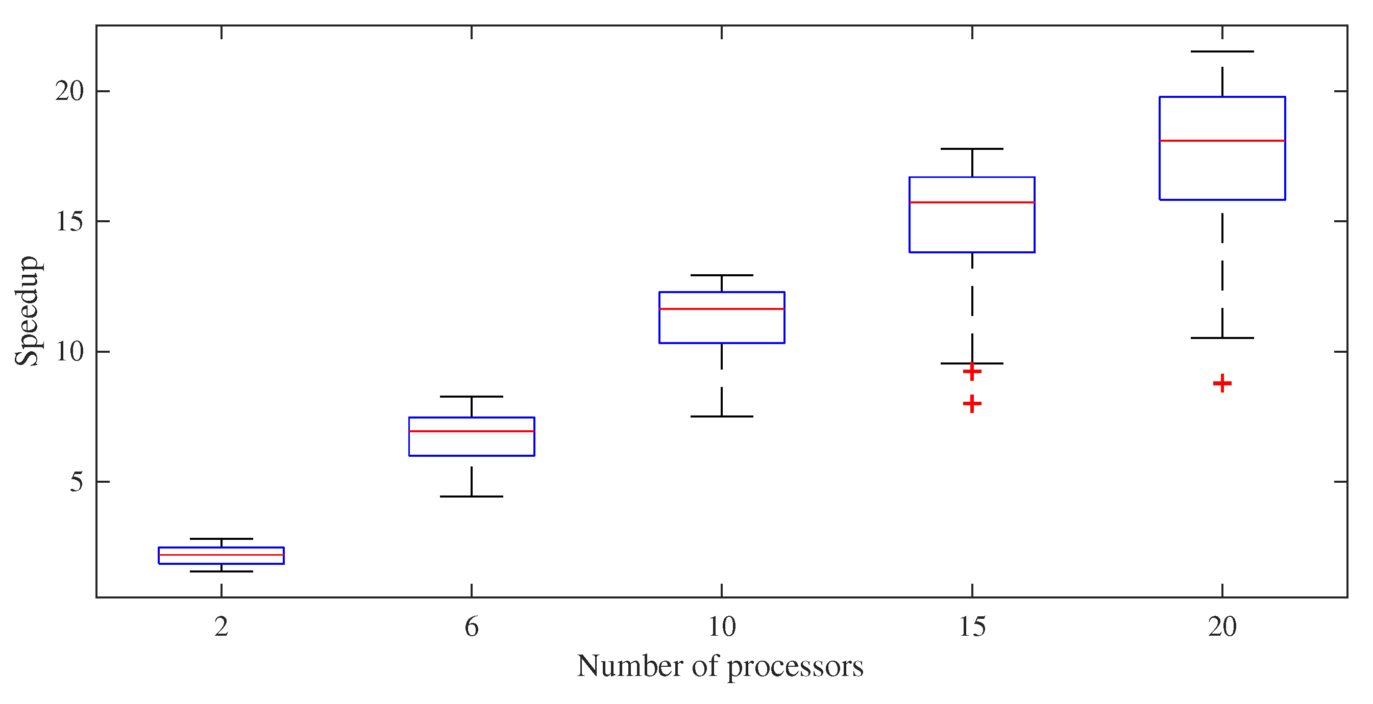
The speedup and efficiency are the two important indices used for the evaluation of parallel processing performance. They are defined as follows:
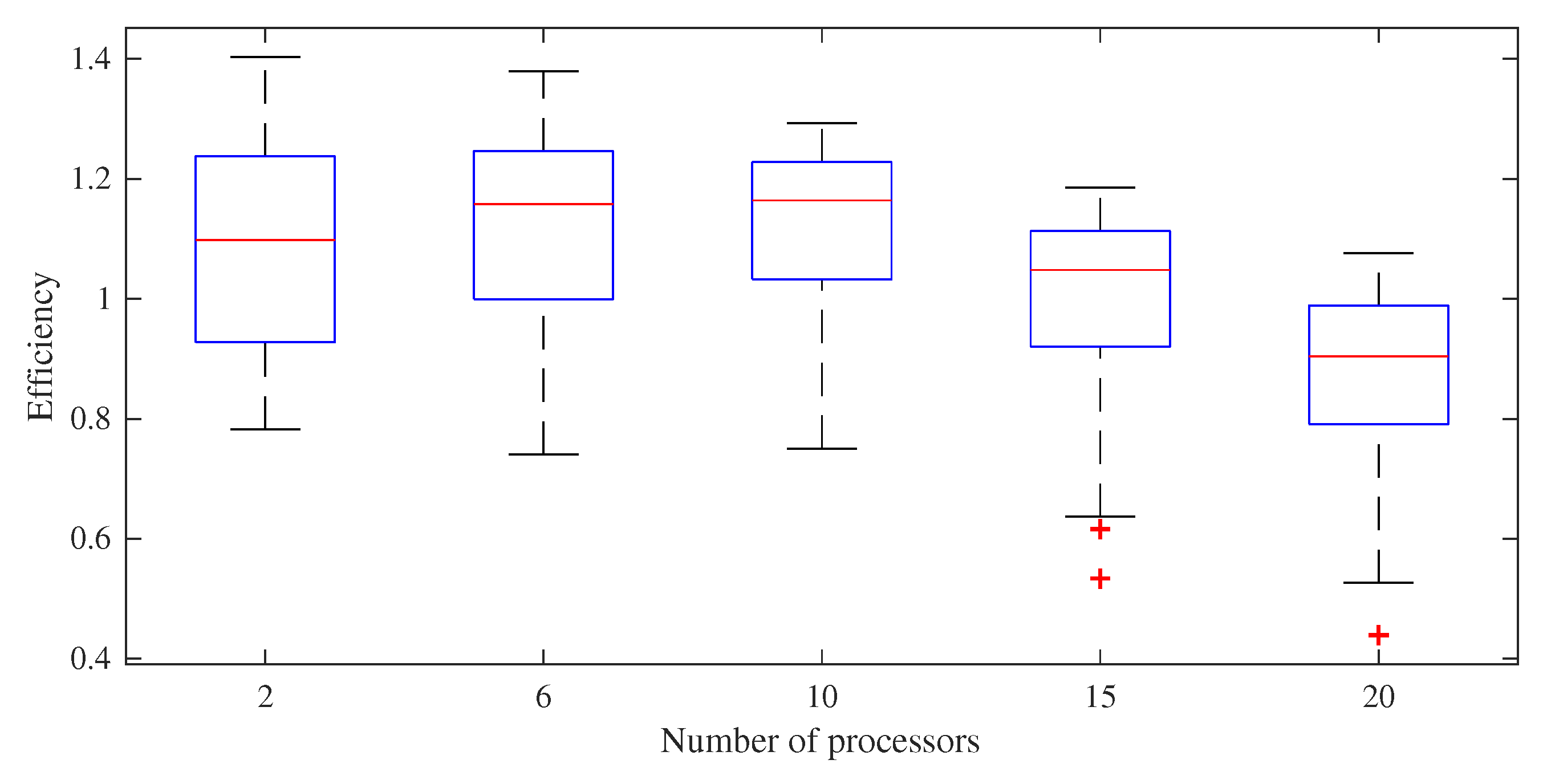
The box plot of the speedup and efficiency are shown in Figure 5 and Figure 6 for each scenario, respectively. The dispersion in speedup increases with the increasing number of processors, as expected. On the other hand, the efficiency of the computation decreases after 10 processors. The speedup and the efficiency behavior for the average computational times are shown in Figure 7 for the scenarios held. The expectation is a linear speedup (or efficiencies less than 1) due to Amdahl’s law [50], which states that the parallel computational speedups may not exceed the linear speedups. As is known, the multi-objective PSO algorithm is based on the search of the solution space by using swarm information. In the application, the total number of iterations is shared by each processor, and the solution space may be searched with the use of more physical sources, which can lead to obtaining solutions faster [51]. It is clear that the speedup increases up to a certain number of processors, then the increasing rate decreases and goes to saturation. We observed a maximum speedup of 17 when 20 processors were used in the simulations. Note that the efficiency decrease after 10 processors is mainly because of the communication overhead between the processors.
5.2. Pareto Solutions
The non-dominated Pareto solutions obtained from 100 independent simulations for each scenario are shown in Figure 8. The relevant regions are zoomed in to provide a clear visualization. The results show that none of the scenarios dominate the others everywhere in the Pareto space; instead, each scenario offers a better near-optimal solution in a different zone. Such a behavior makes it challenging to identify the optimum number of processors providing the best Pareto distribution. Therefore, we need some indices to quantify the quality of the solutions obtained by the different numbers of processors. In this regard, the DP, spacing metric (SM), and HV indices were used to compare the performance of the solutions in finding near-optimal solutions over a wide range of the Pareto space.
5.2.1. Domination Percentage
The DP [9] provides information about the quality and convergence of the solutions. For example, given two sets of solutions, and , DP(, ) refers to the percentage of solutions in that are dominated by at least one solution in .
The DP metric results are shown in Table 3, where the entries in each row show the percentage of the solutions of that set that are dominated by the solutions of the set corresponding to the column. According to the numerical results, the Pareto set of the two-processor case shows the highest domination percentage, while their domination by other cases is minimum. That is, the entries in Column #2 are the maximum values in their corresponding rows, and the entries in Row #2 are the minimum values in their related columns. In this regard, the solutions of the 2-processor case dominate 65%, 80%, 81%, 90%, and 89% of the solutions corresponding to the 1-processor, 6-processor, 10-processor, 10-processor, 15-processor, and 20-processor cases, respectively. On the other hand, the maximum domination of the solutions of the two-processor case is 22%. Another interesting result is that the domination percentages of the solution sets decrease with the increasing number of processors, with one exception. In summary, the two-processor solutions reduce the average computational time of the serial case by 53%, while showing the highest domination percentage (better Pareto quality in the sense of domination percentage). This is followed by the six-processor solution set. The worst one is the 20-processor solution set. At this point, it is worth saying that the domination percentage compares the solution set, but does not quantify the quality differences between the solution sets.
5.2.2. Spacing Metric
An estimate of how evenly non-dominated solutions are distributed in the Pareto front space is provided by this metric. The spacing metric (SM) computes a relative distance measure between consecutive non-dominated solutions in the obtained set based on the distribution of vectors. Note that the small SM corresponds to closely distributed solutions in the Pareto front space, and the solutions’ quality is better.
Based on the average spacing metric values in Table 4, the best case providing the most-uniform Pareto distribution is the two-processor scenario with an average SM value of 0.0063. It is followed by the serial configuration and six-processor scenarios. One can again realize that the SM values get worse for the increasing number of processors. On the other hand, the two-processor scenario shows the lowest standard deviation, indicating more uniform solutions. The relative standard deviations of the other scenarios (standard deviation/average value) are all around 50%.
5.2.3. Hypervolume Index
The volume of a Pareto space dominated by a set of non-dominated solutions is computed by the HV index. Each scenario’s HV index gives us a clear idea of the convergence and diversity of the non-dominated solutions. Note that higher values of the HV mean that the solution set is closer to an optimal Pareto set and may also indicate a more uniform distribution of solutions in the Pareto space.
The results of the HV index statistics for the different processor scenarios are shown in Table 5. The highest average HV index is 0.1882 for simulations using two processors. It is followed by the 20-processor and 10-processor cases. The worst one is the serial computation case. The two-processor case also shows the minimum standard deviation, indicating more evenly distributed Pareto fronts in 100 simulations.
5.2.4. Pareto Solution Candidate and Corresponding Values
The Pareto-optimal solutions for each scenario are shown in Figure 9. A specific solution within the cost values of USD 0.580 and 0.587 million is shown in red color for each scenario. This solution that will be used to compare the scenarios from the point of objective values and optimal DG allocations and sizing will be called the Pareto solution candidate (PSC). In comparison, PSC-x refers to the PSC of the x-processor case, and the base case is the scenario where there is no DG considered in the system. The locations, types, and sizes of the DG units are shown in Table 6. The total size (cost) and energy losses are also illustrated in the table.
One can easily realize that all PSCs utilize WT-type distributed generation units besides a relatively small PV unit in PSC-20. This is mainly because of high WT outputs compared to PV systems during fall and winter (See Figure 3b,c) in the region. Although there are some differences between the locations of installed units, the distribution of DG units seems reasonable when considering the branches as a whole. Due to the number of buses and bus loads, in all scenarios, branches between bus-7 and bus-18 and between bus-26 and bus-33 accommodate most of the distributed generation units, while the branch between bus-19 and bus-22 does not need any DG supply. The total DG size for all cases is between 4190 kW and 4240 kW, showing no more than 2% of differences. If the results are evaluated together, we can conclude that the allocation and sizing of the units for the PSC of different scenarios can be considered to be similar to the serial case.
Since the cost of PSCs is almost kept constant, comparisons were made from the point of power and energy losses of different scenarios. The total energy loss along 72 h was 10.453 MWh (4.6% of the energy consumption) for the base case operating conditions. The energy loss improvements of the cases are 4.329 MWh (1.9%), 4.329 MWh (1.9%), 4.326 MWh (1.9%), 4.324 MWh (1.9%), 4.321 MWh (1.9%), and 4.322 MWh (1.9%) for the PSCs of the 1-, 2-, 6-, 10-, 15-, and 20-processor scenarios, respectively. The improvements of PCSs in power losses are illustrated in Figure 10. Based on the simulation results, all the PSCs reduce the power losses compared to the base case. PSC1 and PSC2 improve the energy losses by 58.5%, PSC6, PSC10, and PSC20 by 58.6%, and PSC15 by 58.7%. We can again conclude that there is an agreement between the energy losses and hourly power losses of PSCs for different scenarios.
Since one of the optimization goals is to satisfy the inequality constraints (eliminate all the voltage violations), the final comparison was performed with respect to the minimum voltage magnitudes of PCSs. The minimum voltage magnitude was originally 0.9131 p.u. for the base case operating conditions without and with installed DGs. The minimum voltage magnitude was found to be 0.9502 p.u for PSC-1 and PSC-15, 0.9505 p.u. for PSC-2 and PSC-6, and 0.9500 p.u. for PSC-10 and PSC-20. From a practical point of view, we can conclude that all the PSCs of different scenarios are successful in eliminating the undervoltage problems.
6. Conclusions
Since there were relatively less efforts on decreasing the computational time in optimal DG allocation and sizing problems, this paper was devoted to decreasing the computational time of the optimization process. Moreover, the relationship between the accuracy and speed of the parallel computation was also analyzed. In this context, a parallel MOPSO computation was applied to the IEEE 33-bus test system, which aims to penetrate DGs into a DN for the minimization of energy losses and annual DG costs.
Six different parallel simulation scenarios, each corresponding to a different number of processors, were tested for the same network and DG configurations. The non-dominated Pareto solutions obtained from 100 independent simulations for each scenario showed that none of the scenarios dominate the others everywhere in the Pareto space. Therefore, three popular indices were used to quantify the quality of the solutions obtained by different numbers of processors. According to the DP, SM, and HV indices, the t-processor case was found to be the best. On the other hand, the Pareto solutions were found to be more dispersed for a higher number of processors. Such a dispersion was concluded to limit the number of processors for practical implementations.
When the optimal locations and sizes of the different scenarios were compared, all the scenarios were found to provide a similar distribution of the DGs and comparable improvements in energy losses around 58% with respect to the base case operating conditions. On the other hand, the efficiency of parallel processing was found to decrease beyond 10 processors.
Note that the system characteristics and constraints used for the proposed methodology are not common in the literature, and different problem constraints affect the results directly. On the other hand, since the paper aimed to speed up the computation process of a single processor and attain dependable solutions, comparisons were made with a single processor case for the selected heuristic algorithm.
Author Contributions
Software, S.Y.; Formal analysis, B.A.; Investigation, B.A. and O.C.; Project administration, A.O. All authors have read and agreed to the published version of the manuscript.
Funding
This study was supported by funding from the “117E773 Advanced Evolutionary Computation for Smart Grid and Smart Community” project, which is a part of the 1001 Project sponsored by TUBITAK, the Turkish Council for Scientific and Technological Research.
Data Availability Statement
Conflicts of Interest
The authors declare no conflict of interest.
References
- Aghaei, J.; Muttaqi, K.M.; Azizivahed, A.; Gitizadeh, M. Distribution expansion planning considering reliability and security of energy using modified PSO (Particle Swarm Optimization) algorithm. Energy 2014, 65, 398–411. [Google Scholar] [CrossRef] [Green Version]
- Kumawat, M.; Gupta, N.; Jain, N.; Bansal, R.C. Swarm-intelligence-based optimal planning of distributed generators in distribution network for minimizing energy loss. Electr. Power Compon. Syst. 2017, 45, 589–600. [Google Scholar] [CrossRef]
- Tan, W.S.; Hassan, M.Y.; Rahman, H.A.; Abdullah, M.P.; Hussin, F. Multi-distributed generation planning using hybrid particle swarm optimisation-gravitational search algorithm including voltage rise issue. IET Gener. Transm. Distrib. 2013, 7, 929–942. [Google Scholar] [CrossRef]
- Yammani, C.; Maheswarapu, S.; Matam, S.K. A Multi-objective Shuffled Bat algorithm for optimal placement and sizing of multi distributed generations with different load models. Int. J. Electr. Power Energy Syst. 2016, 79, 120–131. [Google Scholar] [CrossRef]
- Abu-Mouti, F.S.; El-Hawary, M.E. Optimal Distributed Generation Allocation and Sizing in Distribution Systems via Artificial Bee Colony Algorithm. IEEE Trans. Power Deliv. 2011, 26, 2090–2101. [Google Scholar] [CrossRef]
- Lalitha, M.P.; Reddy, V.V.; Usha, V. Optimal DG Placement for Minimum Real Power Loss in Radial Distribution Systems Using PSO. J. Theor. Appl. Inf. Technol. 2010, 13, 108. [Google Scholar]
- Borges, C.L.T.; Falcao, D.M. Impact of distributed generation allocation and sizing on reliability, losses and voltage profile. In Proceedings of the 2003 IEEE Bologna Power Tech Conference Proceedings, Bologna, Italy, 23–26 June 2003; Volume 2, p. 5. [Google Scholar]
- Javed, H.; Muqeet, H.A.; Shehzad, M.; Jamil, M.; Khan, A.A.; Guerrero, J.M. Optimal energy management of a campus microgrid considering financial and economic analysis with demand response strategies. Energies 2021, 14, 8501. [Google Scholar] [CrossRef]
- Ahmadi, B.; Ceylan, O.; Ozdemir, A. Distributed energy resource allocation using multi-objective grasshopper optimization algorithm. Electr. Power Syst. Res. 2021, 201, 107564. [Google Scholar] [CrossRef]
- Nusair, K.; Alhmoud, L. Application of equilibrium optimizer algorithm for optimal power flow with high penetration of renewable energy. Energies 2020, 13, 6066. [Google Scholar] [CrossRef]
- Ahmadi, B.; Ceylan, O.; Ozdemir, A. Grey wolf optimizer for allocation and sizing of distributed renewable generation. In Proceedings of the 2019 54th International Universities Power Engineering Conference (UPEC), Bucharest, Romania, 3–6 September 2019; pp. 1–6. [Google Scholar] [CrossRef]
- Chiang, M.Y.; Huang, S.C.; Hsiao, T.C.; Zhan, T.S.; Hou, J.C. Optimal Sizing and Location of Photovoltaic Generation and Energy Storage Systems in an Unbalanced Distribution System. Energies 2022, 15, 6682. [Google Scholar] [CrossRef]
- Dharavat, N.; Sudabattula, S.K.; Velamuri, S.; Mishra, S.; Sharma, N.K.; Bajaj, M.; Elgamli, E.; Shouran, M.; Kamel, S. Optimal Allocation of Renewable Distributed Generators and Electric Vehicles in a Distribution System Using the Political Optimization Algorithm. Energies 2022, 15, 6698. [Google Scholar] [CrossRef]
- Yang, Y.; Wei, Q.; Liu, S.; Zhao, L. Distribution Strategy Optimization of Standalone Hybrid WT/PV System Based on Different Solar and Wind Resources for Rural Applications. Energies 2022, 15, 5307. [Google Scholar] [CrossRef]
- Schultz, H.S.; Carvalho, M. Design, Greenhouse Emissions, and Environmental Payback of a Photovoltaic Solar Energy System. Energies 2022, 15, 6098. [Google Scholar] [CrossRef]
- Li, X.; Jones, G. Optimal Sizing, Location, and Assignment of Photovoltaic Distributed Generators with an Energy Storage System for Islanded Microgrids. Energies 2022, 15, 6630. [Google Scholar] [CrossRef]
- Wang, Y.; Huang, Y.; Wang, Y.; Li, F.; Zhang, Y.; Tian, C. Operation optimization in a smart micro-grid in the presence of distributed generation and demand response. Sustainability 2018, 10, 847. [Google Scholar] [CrossRef] [Green Version]
- Majidi, M.; Ozdemir, A.; Ceylan, O. Optimal DG allocation and sizing in radial distribution networks by Cuckoo search algorithm. In Proceedings of the 2017 19th International Conference on Intelligent System Application to Power Systems (ISAP), San Antonio, TX, USA, 17–20 September 2017; pp. 1–6. [Google Scholar] [CrossRef]
- Sultana, U.; Khairuddin, A.B.; Mokhtar, A.; Zareen, N.; Sultana, B. Grey wolf optimizer based placement and sizing of multiple distributed generation in the distribution system. Energy 2016, 111, 525–536. [Google Scholar] [CrossRef]
- Ayalew, M.; Khan, B.; Giday, I.; Mahela, O.P.; Khosravy, M.; Gupta, N.; Senjyu, T. Integration of Renewable Based Distributed Generation for Distribution Network Expansion Planning. Energies 2022, 15, 1378. [Google Scholar] [CrossRef]
- Ahmadi, B.; Ceylan, O.; Ozdemir, A. Impacts of Load and Generation Volatilities on the Voltage Profiles Improved by Distributed Energy Resources. In Proceedings of the 2020 55th International Universities Power Engineering Conference (UPEC), Turin, Italy, 1–4 September 2020; pp. 1–6. [Google Scholar]
- Nekooei, K.; Farsangi, M.M.; Nezamabadi-Pour, H.; Lee, K.Y. An improved multi-objective harmony search for optimal placement of DGs in distribution systems. IEEE Trans. Smart Grid 2013, 4, 557–567. [Google Scholar] [CrossRef]
- Dias Santos, J.; Marques, F.; Garcés Negrete, L.P.; Andrêa Brigatto, G.A.; López-Lezama, J.M.; Muñoz-Galeano, N. A Novel Solution Method for the Distribution Network Reconfiguration Problem Based on a Search Mechanism Enhancement of the Improved Harmony Search Algorithm. Energies 2022, 15, 2083. [Google Scholar] [CrossRef]
- Hadidian-Moghaddam, M.J.; Arabi-Nowdeh, S.; Bigdeli, M.; Azizian, D. A multi-objective optimal sizing and siting of distributed generation using ant lion optimization technique. Ain Shams Eng. J. 2018, 9, 2101–2109. [Google Scholar] [CrossRef]
- Abul’Wafa, A.R. Ant-lion optimizer-based multi-objective optimal simultaneous allocation of distributed generations and synchronous condensers in distribution networks. Int. Trans. Electr. Energy Syst. 2019, 29, e2755. [Google Scholar] [CrossRef]
- VC, V.R. Ant Lion optimization algorithm for optimal sizing of renewable energy resources for loss reduction in distribution systems. J. Electr. Syst. Inf. Technol. 2018, 5, 663–680. [Google Scholar]
- Hinneck, A.; Pozo, D. Optimal Transmission Switching: Improving Exact Algorithms by Parallel Incumbent Solution Generation. IEEE Trans. Power Syst. 2022, 1–14. [Google Scholar] [CrossRef]
- Zhang, X.; Chen, W.; Dai, C.; Cai, W. Dynamic multi-group self-adaptive differential evolution algorithm for reactive power optimization. Int. J. Electr. Power Energy Syst. 2010, 32, 351–357. [Google Scholar] [CrossRef]
- Angulo, A.; Rodríguez, D.; Garzón, W.; Gómez, D.F.; Al Sumaiti, A.; Rivera, S. Algorithms for bidding strategies in local energy markets: Exhaustive search through parallel computing and metaheuristic optimization. Algorithms 2021, 14, 269. [Google Scholar] [CrossRef]
- Rodríguez-García, J.; Ribó-Pérez, D.; Álvarez Bel, C.; Peñalvo-López, E. Maximizing the Profit for Industrial Customers of Providing Operation Services in Electric Power Systems via a Parallel Particle Swarm Optimization Algorithm. IEEE Access 2020, 8, 24721–24733. [Google Scholar] [CrossRef]
- Tsai, C.-F.; Dao, T.-K.; Pan, T.-S.; Nguyen, T.-T.; Chang, J.-F. Parallel bat algorithm applied to the economic load dispatch problem. J. Internet Technol. 2016, 17, 761–769. [Google Scholar]
- Ceylan, O.; Liu, G.; Tomsovic, K. Parallel harmony search based distributed energy resource optimization. In Proceedings of the 2015 18th International Conference on Intelligent System Application to Power Systems (ISAP), Porto, Portugal, 11–16 September 2015; pp. 1–6. [Google Scholar] [CrossRef]
- Alba, E. Parallel Evolutionary Computations; Springer: Berlin/Heidelberg, Germany, 2006; Volume 22. [Google Scholar]
- Shigeto, Y.; Sakai, M. Parallel computing of discrete element method on multi-core processors. Particuology 2011, 9, 398–405. [Google Scholar] [CrossRef]
- Fox, G.C.; Williams, R.D.; Messina, G.C. Parallel Computing Works! Elsevier: Amsterdam, The Netherlands, 2014. [Google Scholar]
- Schmidberger, M.; Morgan, M.; Eddelbuettel, D.; Yu, H.; Tierney, L.; Mansmann, U. State-of-the-art in Parallel Computing with R. J. Stat. Softw. 2009. [Google Scholar] [CrossRef] [Green Version]
- Salleh, S.; Zomaya, A.Y. Scheduling in Parallel Computing Systems: Fuzzy and Annealing Techniques; Springer Science & Business Media: New York, NY, USA, 2012; Volume 510. [Google Scholar]
- Scarcello, L.; Giordano, A.; Mastroianni, C. Edge Computing Parallel Approach for Efficient Energy Sharing in a Prosumer Community. Energies 2022, 15, 4543. [Google Scholar] [CrossRef]
- Eager, D.L.; Zahorjan, J.; Lazowska, E.D. Speedup versus efficiency in parallel systems. IEEE Trans. Comput. 1989, 38, 408–423. [Google Scholar] [CrossRef] [Green Version]
- Ahmadi, B.; Ceylan, O.; Ozdemir, A.; Fotuhi-Firuzabad, M. A multi-objective framework for distributed energy resources planning and storage management. Appl. Energy 2022, 314, 118887. [Google Scholar] [CrossRef]
- Rana, A.; Darji, J.; Pandya, M. Backward/forward sweep load flow algorithm for radial distribution system. Int. J. Sci. Res. Dev. 2014, 2, 398–400. [Google Scholar]
- Nebro, A.J.; Durillo, J.J.; Garcia-Nieto, J.; Coello Coello, C.A.; Luna, F.; Alba, E. SMPSO: A new PSO-based metaheuristic for multi-objective optimization. In Proceedings of the 2009 IEEE Symposium on Computational Intelligence in Multi-Criteria Decision-Making(MCDM), Nashville, TN, USA, 30 March–2 April 2009; pp. 66–73. [Google Scholar] [CrossRef]
- Wang, D.; Tan, D.; Liu, L. Particle swarm optimization algorithm: An overview. Soft Comput. 2018, 22, 387–408. [Google Scholar] [CrossRef]
- Censor, Y. Pareto optimality in multiobjective problems. Appl. Math. Optim. 1977, 4, 41–59. [Google Scholar] [CrossRef]
- Younesi, S.; Ahmadi, B.; Ceylan, O.; Ozdemir, A. Allocation of Distributed Generators Using Parallel Grey Wolf Optimization. Mod. Power Syst. 2021, 22, 387–408. [Google Scholar]
- Baran, M.; Wu, F. Network reconfiguration in distribution systems for loss reduction and load balancing. IEEE Trans. Power Deliv. 1989, 9, 101–102. [Google Scholar]
- EPIAS. EPIAS Transparency Platform. Available online: https://seffaflik.epias.com.tr/transparency/index.xhtml (accessed on 3 June 2022).
- Intel. Intel Xeon Processor. Available online: https://ark.intel.com/content/www/us/en/ark/products/91754/intel-xeon-processor-e5-2680-v4-35m-cache-2-40-ghz.html (accessed on 3 June 2022).
- Sharma, G.; Martin, J. MATLAB®: A language for parallel computing. Int. J. Parallel Program. 2009, 37, 3–36. [Google Scholar] [CrossRef] [Green Version]
- Amdahl, G.M. Validity of the Single Processor Approach to Achieving Large Scale Computing Capabilities, Reprinted from the AFIPS Conference Proceedings, Vol. 30 (Atlantic City, N.J., Apr. 18–20), AFIPS Press, Reston, Va., 1967, pp. 483–485, when Dr. Amdahl was at International Business Machines Corporation, Sunnyvale, California. IEEE Solid-State Circuits Soc. Newsl. 2007, 12, 19–20. [Google Scholar] [CrossRef]
- Alba, E. Parallel evolutionary algorithms can achieve super-linear performance. Inf. Process. Lett. 2002, 82, 7–13. [Google Scholar] [CrossRef]
Figure 1.
The flow chart of the parallel multi-objective PSO algorithm.

Figure 2.
The line diagram of the 33-bus test system.

Figure 3.
Load-, PV-, and WT-scaled outputs for different seasons of the year.

Figure 4.
Average computational times of the scenarios.

Figure 5.
Box plot of the speedup results.

Figure 6.
Box plot of the efficiency results.

Figure 7.
Speedup and efficiency versus number of processors.

Figure 8.
Non-dominated Pareto solutions for different scenarios.

Figure 9.
The non-dominated Pareto solutions for different numbers of processors and PSCs.

Figure 10.
The active power losses for PSCs.


Table 1.
DG parameters [9].
Table 1.
DG parameters [9].
| Max DG number | 8 | (USD/kW) | 1830 |
| DG types | 2 | (USD/kW) | 1600 |
| (year) | 30 | (USD/kW-yr) | 18 |
| (year) | 25 | (USD/kW-yr) | 25 |
Table 2.
Computation time statistics for each scenario.
| # Processor | Average | STD | Min | Max |
|---|---|---|---|---|
| 1 | 4886 | 414 | 4405 | 6115 |
| 2 | 2297 | 372 | 1741 | 3122 |
| 6 | 745 | 120 | 590 | 1100 |
| 10 | 448 | 67 | 378 | 651 |
| 15 | 338 | 70 | 275 | 610 |
| 20 | 290 | 66 | 227 | 557 |
Table 3.
Domination percentage metric for the Pareto solutions of different scenarios.
| x | DP(x,1) | DP(x,2) | DP(x,6) | DP(x,10) | DP(x,15) | DP(x,20) |
|---|---|---|---|---|---|---|
| 1 | 65 | 39 | 26 | 21 | 17 | |
| 2 | 22 | 18 | 13 | 9 | 6 | |
| 6 | 53 | 80 | 25 | 35 | 11 | |
| 10 | 61 | 81 | 68 | 39 | 22 | |
| 15 | 65 | 90 | 60 | 52 | 29 | |
| 20 | 73 | 89 | 74 | 61 | 47 |
Table 4.
SM statistics of Pareto solutions for different scenarios.
| # Processor | Average | STD | Min | Max |
|---|---|---|---|---|
| 1 | 0.0088 | 0.0036 | 0.0030 | 0.0195 |
| 2 | 0.0063 | 0.0022 | 0.0038 | 0.0158 |
| 6 | 0.0082 | 0.0041 | 0.0032 | 0.0281 |
| 10 | 0.0100 | 0.0048 | 0.0034 | 0.0261 |
| 15 | 0.0105 | 0.0053 | 0.0030 | 0.0283 |
| 20 | 0.0111 | 0.0049 | 0.0028 | 0.0299 |
Table 5.
HV results for Pareto solution found in different scenarios.
| # Processor | Average | STD | Min | Max |
|---|---|---|---|---|
| 1 | 0.1688 | 0.0048 | 0.1533 | 0.1759 |
| 2 | 0.1882 | 0.0040 | 0.1777 | 0.1953 |
| 6 | 0.1805 | 0.0048 | 0.1664 | 0.1890 |
| 10 | 0.1839 | 0.0042 | 0.1752 | 0.1916 |
| 15 | 0.1735 | 0.0045 | 0.1607 | 0.1828 |
| 20 | 0.1850 | 0.0042 | 0.1756 | 0.1931 |
Table 6.
The units’ size and location for the PSCs.
| PSC-1 | PSC-2 | PSC-6 | ||||||
|---|---|---|---|---|---|---|---|---|
| Type | Location | Size (kW) | Type | Location | Size (kW) | Type | Location | Size (kW) |
| WT | 8 | 500 | WT | 10 | 530 | WT | 8 | 500 |
| WT | 13 | 830 | WT | 14 | 650 | WT | 13 | 810 |
| WT | 18 | 490 | WT | 17 | 530 | WT | 18 | 500 |
| WT | 25 | 460 | WT | 25 | 480 | WT | 25 | 410 |
| WT | 30 | 920 | WT | 30 | 1000 | WT | 30 | 1000 |
| WT | 32 | 1000 | WT | 32 | 1000 | WT | 32 | 1000 |
| Total unit size (kW) | 4200 | 4190 | 4220 | |||||
| Total losses (kWh) | 4329 | 4329 | 4326 | |||||
| PSC-10 | PSC-15 | PSC-20 | ||||||
| Type | Location | Size (kW) | Type | Location | Size (kW) | Type | Location | Size (kW) |
| WT | 10 | 700 | WT | 12 | 500 | PV | 8 | 150 |
| WT | 16 | 1000 | WT | 14 | 490 | WT | 13 | 1000 |
| WT | 25 | 590 | WT | 18 | 590 | WT | 17 | 590 |
| WT | 30 | 940 | WT | 25 | 680 | WT | 25 | 500 |
| WT | 32 | 1000 | WT | 30 | 1000 | WT | 30 | 1000 |
| WT | 33 | 980 | WT | 32 | 1000 | |||
| Total unit size (kW) | 4230 | 4240 | 4240 | |||||
| Total losses (kWh) | 4324 | 4321 | 4322 | |||||
Publisher’s Note: MDPI stays neutral with regard to jurisdictional claims in published maps and institutional affiliations. |
© 2022 by the authors. Licensee MDPI, Basel, Switzerland. This article is an open access article distributed under the terms and conditions of the Creative Commons Attribution (CC BY) license (https://creativecommons.org/licenses/by/4.0/).
Share and Cite
MDPI and ACS Style
Younesi, S.; Ahmadi, B.; Ceylan, O.; Ozdemir, A. Optimum Parallel Processing Schemes to Improve the Computation Speed for Renewable Energy Allocation and Sizing Problems. Energies 2022, 15, 9301. https://doi.org/10.3390/en15249301
AMA Style
Younesi S, Ahmadi B, Ceylan O, Ozdemir A. Optimum Parallel Processing Schemes to Improve the Computation Speed for Renewable Energy Allocation and Sizing Problems. Energies. 2022; 15(24):9301. https://doi.org/10.3390/en15249301
Chicago/Turabian StyleYounesi, Soheil, Bahman Ahmadi, Oguzhan Ceylan, and Aydogan Ozdemir. 2022. "Optimum Parallel Processing Schemes to Improve the Computation Speed for Renewable Energy Allocation and Sizing Problems" Energies 15, no. 24: 9301. https://doi.org/10.3390/en15249301
Note that from the first issue of 2016, this journal uses article numbers instead of page numbers. See further details here.