
A Deep Neural Network as a Strategy for Optimal Sizing and Location of Reactive Compensation Considering Power Consumption Uncertainties


Smart Grid Research Group—GIREI (Spanish Acronym), Salesian Polytechnic University, Quito EC170702, Ecuador
*
Author to whom correspondence should be addressed.
Energies 2022, 15(24), 9367; https://doi.org/10.3390/en15249367
Submission received: 8 November 2022
/
Revised: 25 November 2022
/
Accepted: 8 December 2022
/
Published: 10 December 2022
(This article belongs to the Special Issue Machine Learning Applications in Power System)
Abstract
:This research proposes a methodology for the optimal location and sizing of reactive compensation in an electrical transmission system through a deep neural network (DNN) by considering the smallest cost for compensation. An electrical power system (EPS) is subjected to unexpected increases in loads which are physically translated as an increment of users in the EPS. This phenomenon decreases voltage profiles in the whole system which also decreases the EPS’s reliability. One strategy to face this problem is reactive compensation; however, finding the optimal location and sizing of this compensation is not an easy task. Different algorithms and techniques such as genetic algorithms and non-linear programming have been used to find an optimal solution for this problem; however, these techniques generally need big processing power and the processing time is usually considerable. That being stated, this paper’s methodology aims to improve the voltage profile in the whole transmission system under scenarios in which a PQ load is randomly connected to any busbar of the system. The optimal location of sizing of reactive compensation will be found through a DNN which is capable of a relatively small processing time. The methodology is tested in three case studies, IEEE 14, 30 and 118 busbar transmission systems. In each of these systems, a brute force algorithm (BFA) is implemented by connecting a PQ load composed of 80% active power and 20% reactive power (which varies from 1 MW to 100 MW) to every busbar, for each scenario, reactive compensation (which varies from 10 Mvar to 300 Mvar) is connected to every busbar. Then power flows are generated for each case and by selecting the scenario which is closest to 90% of the original voltage profiles, the optimal scenario is selected and overcompensation (which would increase cost) is avoided. Through the BFA, the DNN is trained by selecting 70% of the generated data as training data and the other 30% is used as test data. Finally, the DNN is capable of achieving a 100% accuracy for location (in all three case studies when compared with BFA) and objective deviation has a difference of 3.18%, 7.43% and 0% for the IEEE 14, 30 and 118 busbar systems, respectively (when compared with the BFA). With this methodology, it is possible to find the optimal location and sizing of reactive compensation for any transmission system under any PQ load increment, with almost no processing time (with the DNN trained, the algorithm takes seconds to find the optimal solution).
1. Introduction
The global growth in electricity consumption due to human and economic activities, including the incorporation of new technologies in the distribution network such as electric cars, charging stations, distributed generation for self-supply and renewable energy, created an industry with new technologies with high reactive content and power electronics, and has led to problems in the distribution and transmission networks, causing a decrease in the quality of services such as low voltages, increased losses in conductors and increased operating costs [1].
Planning in the operation and expansion of electrical systems must consider these changes and one of the current and practical tools to improve the technical and economic operating conditions of power systems is reactive power compensation.
Reactive power compensation, whether based on FACTS devices or capacitor banks, provides benefits in the operation of networks when the compensators are installed in an adequate place and with an optimum capacity. Thus, several research works have been developed with optimization algorithms, some focused only on finding the optimal location and others to additionally determine the size of the compensator. Among the optimized variables considered in these works, most researchers consider reducing active power losses and improving the power factor and voltage profiles, as well as reducing operating costs and installation of these devices [2].
1.1. Literature Review
Electric power systems have become increasingly large and complex, and their operation in terms of voltage stability is at its limit with a small safety margin, which is why this research’s literature review shows different classical optimization techniques applied to reactive power compensation and new techniques based on autonomous learning that are applied to solve the problems that arise in distribution and transmission networks (especially focusing on voltage profiles improvement and losses reduction).
In [3], a detailed analysis of the different objectives that are pursued in the distribution and transmission systems regarding sizing and optimal placement of reactive power compensation devices is shown. This research also indicates existing technologies related to FACTS as well as the different optimization criteria to improve the operating and economic conditions of the EPS.
In [1], new techniques that have been developed in machine learning are shown, the most important techniques are ANN (artificial neural networks) in combination with control techniques such as fuzzy control. This research focuses on stability improvement by locating reactive compensation in the electrical power system.
The research in [4] analyzes the location and sizing of FACTS compensators, specifically D-STATCOMP, using a hybrid heuristic combining the algorithm based on the prey targeting behaviour of whales and grey wolf optimization. The methodology is tested in distribution systems for power quality improvement and voltage stability and its performance is compared with conventional optimization methods GA, ABC, PSO, GWO and WOA to determine its effectiveness.
In [5], the authors use particle swarm optimization (PSO) to determine the capacity and location of capacitor banks to guarantee the operation of a microgrid under minimum cost criteria, improving the power factor and reducing the maximum and average voltage deviations of the system.
BCC capacitor banks for reactive compensation in distribution systems that are used to improve power factor, power losses reduction and minimization of annual operating cost are discussed in [2]. This research proposes a hybrid method based on particle swarm optimization together with a particle swarm gravitational search algorithm (PSOGSA) as an optimization mechanism to solve the problem of optimal BCC allocation with minimization of annual operating cost and improvement of system power quality and propose a voltage-loss cost index (VLCI) as an allocation mechanism. The methodology is tested in the 33- and 69-bus radial systems, as well as on a real distribution network of 111 nodes in Moscow.
In [6], the location and sizing of the UPQC power quality conditioner are proposed, considering the reconfiguration of the distribution network for loss reduction all under an exhaustive search. The model is tested in a radial-type network of 69 nodes.
In [7], a convex-genetic method is proposed to determine the location and size of a D-STATCOM to reduce power losses and minimize the annual operating costs of a 33-node radial distribution network. The results show a processing time for the algorithm of 3.11 h.
The investigation in [8] shows a transmission system planning strategy that considers the optimization of several costs, among them, active power losses, reactive power generation, FACTS devices and transmission line loadability, through a probabilistic hybridization of the crow search algorithm and JAYA. The heuristic is validated in two test systems of 30 and 75 nodes.
In [9], the research uses the dolphin algorithm to determine the location and size of reactive compensation in 16- and 33-busbar distribution networks under different models for various types of loads (constant and mixed power, current and impedance), minimizing power losses and voltage drops between nodes.
In [10], a methodology is presented to optimize the cost/benefit ratio in the installation of FACTS in distribution networks employing a differential evolution algorithm considering the lowest capacity and cost of the FACT device and minimizing the power losses in the network. The methodology is evaluated in systems of 30, 33 and 69 nodes.
In [11], the research proposes a heuristic that considers the modified artificial bee colony algorithm for optimal reactive compensation placement through UPQC to improve the power quality of the IEEE 30-node network and compares the results with other methods such as PSO and the genetic algorithm.
In [12,13], a planning methodology is established for the simultaneous location of reactive compensation devices, specifically the OUPQC with its series and shunt units (SEU and SHU) using the Cuckoo search algorithm and load growth. The methodology is tested in the 69-node IEEE network in steady state and the results are effective in improving the quality of the network in economic and technical terms.
In [14], the location of reactive compensation in an electrical power system is established and analyzed by employing deep neural networks to improve the voltage profile in each of the nodes of the evaluated systems (14, 30 and 118 nodes). The standard deviation of all voltage profiles over a referential value is evaluated to determine the power flows and training data of the neural network and finally to determine the optimal location of the reactive compensation.
In [15], an application based on fuzzy logic and bio-genetic algorithms is established to help decision-making in the field of operation and reactive power compensation of an islanded power grid. The research’s objective is to improve power quality in terms of power factor, voltages and loss reduction.
In [16], the planning of transmission networks to improve long-term operating conditions is analyzed by using probabilistically modelling of load scenarios as well as capital and operating costs in the face of massive installation of FACTS devices to minimize generation cost. The heuristic algorithm consists of a sequence of quadratic schedules solved by CPLEX and tested on the IEEE 30-bus system and extended to a 2736-bus model in Poland.
In [17], a methodology is established to compensate for the reactive power by minimizing the total harmonic distortion of voltage and current as well as the installation cost of the passive filter. The optimization problem is solved with a learning algorithm and Pareto distribution.
The work in [18] presents a methodology for optimal reactive power compensation in electrical microgrids using a multi-criteria decision algorithm based on heuristic methods.
Research in [19] presents a model to solve capacitor allocation considering PV penetration and feeder reconfiguration simultaneously in a distribution network minimizing capacitor costs and power losses. The model uses PSO to solve the allocation problem and is tested on a 33-node IEEE network.
In [20], a heuristic based on the whale optimization algorithm is proposed for the optimal placement, sizing and coordination of FACTS devices, specifically TCSC, SVC and UPFC. In the transmission network, the management of the algorithm allows for minimizing operating costs, energy losses and voltage deviations, and is further compared with genetic algorithm (GA) and particle swarm optimization (PSO). The research results show that the total system operating costs and transmission line losses were significantly reduced with the WOA method compared with existing meta-heuristic optimization techniques.
In [21], the research compares a probability-based heuristic with an artificial neural network for optimal sizing and location of distributed generation arrays and flexible AC transmission systems to improve DG-FACTS for operation improvement of two 9-bus and 57-bus systems. The results show that the neural network is more efficient in terms of DG-FACTS capacity sizing compared to the heuristic.
In [22], three different evolutionary techniques, the big bang–big crunch algorithm, gravitational search algorithm and bacterial foraging algorithm are used in conjunction to train and validate an ANN. This research’s strategy manages reactive power and corrects the voltage profile. Additionally, as a study case, the IEEE 30 busbar system was used. The results showed an improvement in the system’s voltage profiles.
As has been stated in this section, reactive compensation has been widely studied and optimal location and sizing have been analyzed with optimization techniques, fuzzy logic and probabilistic logic, among others. However, all those techniques need considerable processing power and their processing time is quite considerable as well. A summary of the main strategies used in the literature review for reactive compensation through optimization algorithms or artificial neural networks is shown in Table 1.
Therefore, this research proposes a methodology which aims to improve the voltage profile in the whole transmission system under scenarios in which a PQ load is randomly connected to any busbar of the system. The optimal location of sizing of reactive compensation will be found through deep neural networks, which require significantly less processing power and are faster than optimization algorithms described in the literature review.
1.2. Organization
This paper is organized into four main sections: Section 1 presents an introduction and literature review of the main techniques, algorithms and methodologies that have been used by other authors for optimal location and sizing for reactive compensation in electrical power systems. Additionally, machine learning techniques and their application for electrical power systems are discussed.
Section 2 fully explains the brute force algorithm which will provide the training and test data for the deep neural network. This section also describes the algorithm restrictions for each case study.
Section 3 shows the resulting values for sizing and location of reactive compensation through the DNN, also these results are compared with the brute force algorithm data which provides the reference values for this paper’s methodology. Additionally, a detailed discussion of each study case is provided in this section.
Finally, Section 4 summarizes the conclusions that this research achieved.
2. Methodology
This work proposes the use of a deep neural network to find the optimal value of reactive compensation and its sizing to improve the voltage profiles in an electrical transmission network. These optimal values will be found in any scenario in which a load of random values with active and reactive components is randomly connected to a node of the electrical transmission network.
The criteria to improve the voltage profiles is based on obtaining a global indicator called objective deviation (it will be further explained in this section) of all the voltage profiles that are at least 90% greater or equal to the original voltage profiles of the system (without additional loads) and seeking the lowest possible cost (using the smallest reactive compensation).
Voltage profiles are obtained by calculating power flows through the Newton–Raphson algorithm, after power flows are calculated values for voltage profiles, angle deviation and active and reactive power are saved in a new matrix which later is used for evaluation of objective deviation and also will be training data for the deep neural network.
This methodology is composed of a brute force algorithm for the generation of electrical network training data, particle swarm optimization to find the deep neural network structure with the best performance, training of the neural network and validation of the results based on the data previously generated.
The methodology is explained in detail in the following sections starting with the study cases.
2.1. Cases of Study
- IEEE 14 busbar transmission system
The IEEE-14 bus system is taken as a case study to test the methodology this research will establish for optimal location and sizing of reactive compensation. This transmission system was developed for research and its aim is to provide mechanisms for the improvement of various electrical parameters involved. The system has 14 busbars, 5 generators and 11 loads.
- IEEE 30 busbar transmission system
The IEEE 30 busbar transmission system is the second transmission system in which the methodology will be tested. This test system represents a real transmission system located in the Midwestern USA. The second study case has 30 busbars, 2 generators and 9 loads.
- IEEE 118 busbar transmission system
Finally, the IEEE 118 busbar transmission system is the third study case for this research. Similarly to the IEEE 30 busbar system, this transmission system also shows a portion of the American Electric Power System located in the Midwestern USA. This system has 118 buses, 19 generators and 91 loads.
2.2. Deep Learning
According to the literature review, deep learning is all the machine learning techniques, algorithms and methodologies that follow a singular structure which resembles how the human nervous system takes and makes decisions. The majority of these techniques have a neural network architecture that extracts features and characteristics from databases to predict and anticipate behaviour in unknown data.
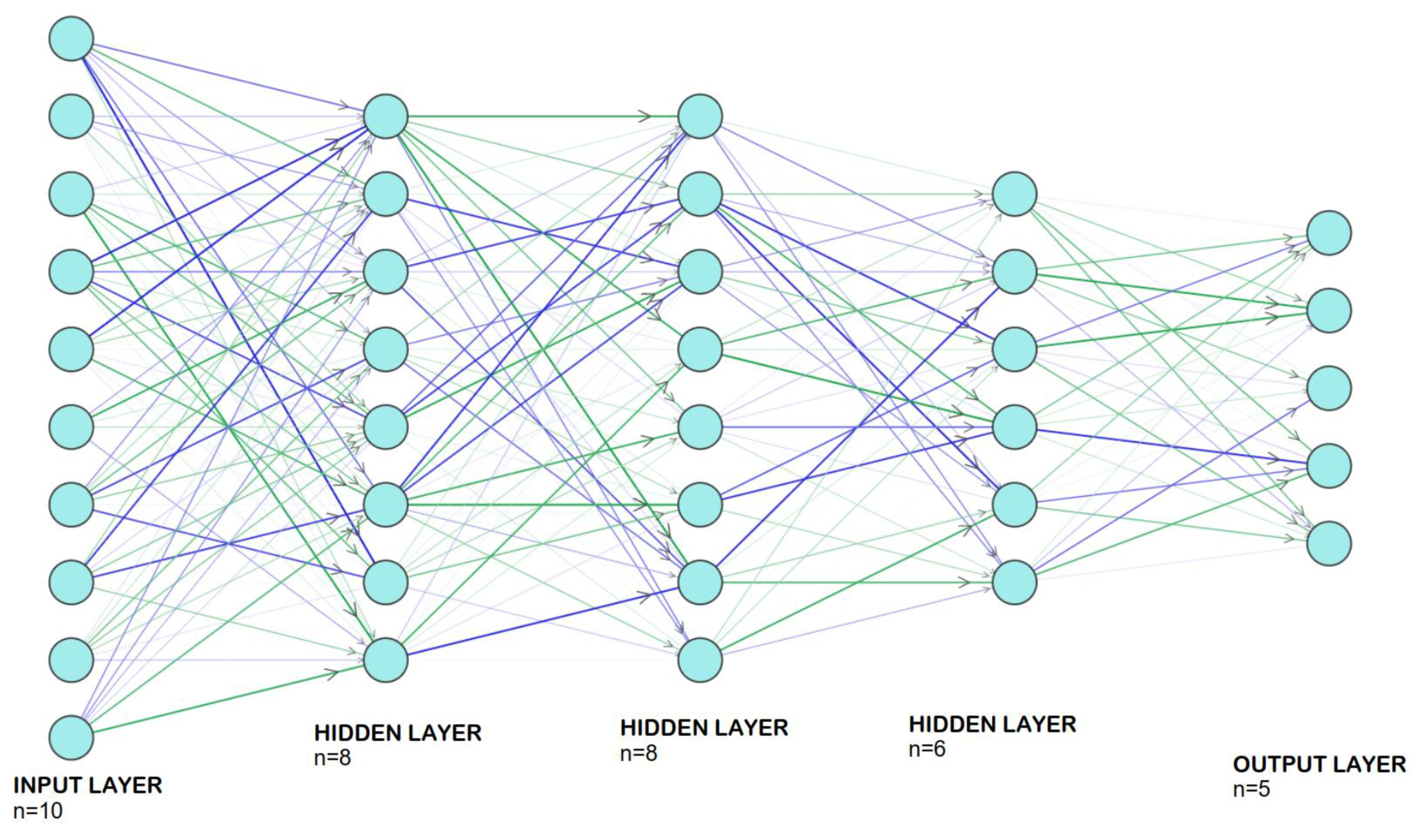
Deep neural networks are composed of layers and neurons, a DNN can have hundreds of hidden layers and similarly, each layer contains a significant number of neurons, this is the reason why a DNN can have a large structure and is known as a deep network. In most cases, neurons in each layer are connected to neurons of the next layer, this connection pattern repeats in all the , as shown in Figure 1, which shows a general structure for a deep neural network and its most important characteristics. Figure 1 is an example in which there are 10 neurons in the input layer, 5 neurons in the output layer and there are three hidden layers with 8, 8 and 6 neurons, respectively.
2.3. Training Data for Deep Neural Network
This work aims to improve the voltage profiles in transmission networks by finding the optimal location and sizing of reactive compensation in transmission systems. For this purpose, certain restrictions have been established that this paper takes as a basis for the proposed algorithm.
2.3.1. Restrictions for the Connection of Randomly Located Loads in the EPS
In the first place, it is proposed that a load can be added randomly to the system in any busbar, said load has an active and reactive component with a ratio of 80% active power and 20% reactive power (load example, P = 10 MW, Q = 2.5 Mvar).
The maximum load values are defined in each test system based on stability criteria. Thus, in the IEEE 14-bar system, the highest load is found at node 3 with a value of 94 MW, and based on a stability analysis it was determined that this load can be increased by up to 220%, reaching a value of 206 MW. For this reason, a limit of 200 MW is established for the load that will be placed randomly in the nodes of the system.
Similarly, in the IEEE 30 busbar system, the highest load corresponding to 94 MW is located at node 5. When performing a stability analysis, it was determined that this load can be increased by up to 190%, reaching a value of 202 MW, by which a limit of 200 MW is established for the load that will be placed randomly in the nodes of the system.
Finally, when analyzing the IEEE system of 118 bars, the highest load corresponds to 130 MW, located at node 80. When performing a stability analysis, it was determined that this load can be increased by up to 180%, reaching a value of 234 MW, which is why a limit of 230 MW is established for the load that will be placed randomly in the nodes of the system. All load restrictions for the study cases are shown in Table 2.
2.3.2. Criteria for Optimal Compensation Sizing and Location Selection
When a load is connected to any busbar of the EPS, all voltage profile levels are decreased in some busbars more than others. When these new voltage profiles are compared to the original ones, it can be inferred that the bigger the additional load connected to the EPS, the bigger the drop for the voltage profiles.
When reactive compensation es connected to a busbar, the effect of the additional load is counteracted and the bigger the compensation the higher the voltage profiles in the compensated system. However, having high voltage profiles is not the most doable strategy because overcompensation might happen and voltage profiles over the security margins might emerge (1.05 (p.u.)). Additionally, the higher the reactive compensation, the higher the cost associated with it.
Since it is impossible to analyze individually every busbar and its voltage profile, this paper uses a modified approach to the standard deviation. This will allow studying all the voltage profiles of the system as a whole. From now on, this criteria will be called objective deviation, and it works by comparing each voltage profile against 1.0 (p.u.), as shown in Equation (1).
Objective deviation will be calculated in the original conditions for every transmission system, then after an additional load is connected to a certain busbar and compensation is applied, the objective deviation will be calculated in this new system. This paper proposes to find the reactive power value and its location that would be able to generate an objective deviation that is at least 90% similar to the original voltages profiles objective deviation.
By following this strategy, the methodology will guarantee that at least the original state of voltage profiles will be reached after a load was randomly located in any busbar also the cost will be the minimum because the smallest value of compensation that reaches the condition (objective deviation) will be selected.
2.3.3. Brute Force Algorithm for Optimal Location and Sizing of Reactive Compensation: Training Data Generation
To generate the training data for the deep neural network, a load with active component P and reactive component Q was added to each bus of the different IEEE test systems. This load is composed of 80% active power and 20% reactive power to represent real-world loads. Scenarios are generated with loads that increase in steps of 1 MW (and their corresponding reactive values) until reaching the maximum value previously established (to avoid instability). This is done in each bar of the electrical power system.
Subsequently, for each added load scenario, reactive compensation scenarios are generated in which reactive compensation is located starting with values of 10 Mvar in steps of 10 Mvar in each busbar and all busbars. This process is detailed in Algorithm 1.
In Algorithm 1, in the first step, the original parameters for each study case are loaded, and for the second step, the original objective deviation is calculated. For the third step, all possible combinations of loads are connected to each busbar. In the fourth step, for each scenario of extra load connected to the system, all possible scenarios of compensation are added to the system. Finally, power flows are calculated and all values are saved.
| Algorithm 1 Brute force algorithm: load connection and compensation for every possible busbar. |
|
For each of the compensation scenarios, power flows are calculated and the objective deviation of each system is evaluated. Based on the objective deviation, whose value is at least 90% greater than or equal to the target deviation before the inclusion of extra loads, the optimal compensation value and its location are found. This process is detailed in Algorithm 2.
In Algorithm 2, in the first step, all the values generated in Algorithm 1 are loaded, and for the second step, objective deviations for each compensation scenario are calculated. For the third step, the best objective deviation is found for each scenario of added load. In the fourth step, the value of compensation for each best objective compensation is extracted. Finally, all values are stored for later use in the deep neural network training.
| Algorithm 2 Brute force algorithm: best compensation location and sizing. |
|
2.3.4. Deep Neural Network Topology: Number of Layers, Neurons and Hyper-Parameters
- The DNN’s hyper-parameters
For every hidden neuron and output, it is necessary to define an activation function, this paper uses rectified linear unit activation functions () as they are the most widely used activation function in the literature review.
For validation, the DNN’s error will be evaluated by the mean square error function () and the smaller the error, the closer the outputs are to the target values provided for the BFA.
A summary of the most important hyper-parameters is shown as follows:
- Activation functions: .
- Error validation function: .
- Epochs for training: 1000.
- Maximum training time: .
- Performance goal for error: 0.
- Training function: .
Number of neurons and layers
Particle swarm optimization was used to find an adequate value for the number of layers NL for the deep neural network and for each layer the number of neurons in that layer is determined as well. Therefore, PSO is used to find the DNN’s topology that has the smallest possible error when regarding the DNN’s performance.
Particle swarm optimization uses operators called particles, the algorithm generates a number of particles i, and each particle has two main characteristics, particle position and particle velocity . Position and velocity indicate how the algorithm will decide the behaviour for the particles corresponding to the next algorithm iteration and how the search process will be carried out [23,24].
In every algorithm’s iteration, each particle saves two “best” values and they are used for calculations in subsequent iterations. The values stored are the best position for each particle and the best position for the whole population in the current iteration . Finally, when the algorithm ends, the best position, which is the solution to the problem, is saved in Gbest [25,26].
Equations (2) and (3) show how to calculate the velocity and position for every particle. Coefficient is the acceleration coefficient for each particle and is the acceleration coefficient for all the particles in an iteration. Additionally, w is a value that is known as inertia.
For the deep neural network, the numbers of layers NL and neurons in each layer are integers, which is why it is necessary to modify the speed update equation to (4), where the random values generated are restricted as integers. In addition, the variables of and take the value of 2 and w the value of 1 (most common values for fast convergence [25]).
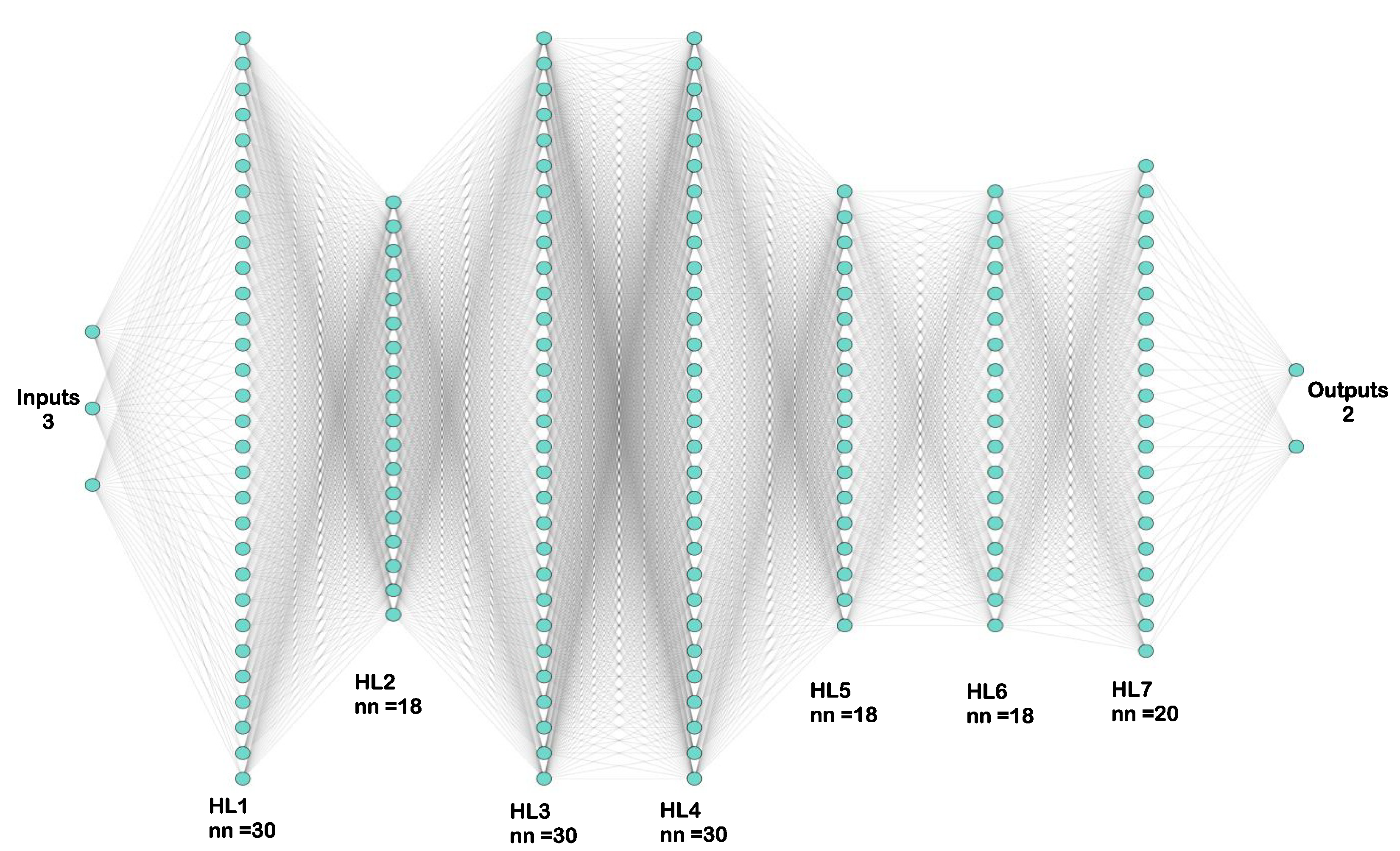
Finally, PSO was implemented considering a population of 500 particles. The topology for the deep neural is shown in Figure 2 and is fully detailed as it follows:
- Inputs: 3, sizing (P and Q) and busbar location for the added load.
- Number of hidden layers: .
- Neurons for the 1st hidden layer: .
- Neurons for the 2nd hidden layer: .
- Neurons for the 3rd hidden layer: .
- Neurons for the 4th hidden layer: .
- Neurons for the 5th hidden layer: .
- Neurons for the 6th hidden layer: .
- Neurons for the 7th hidden layer: .
- Inputs: 2, reactive compensation sizing (Q) and busbar location.
3. Analysis of Results
3.1. Case Study: IEEE 14 Busbar System
When applying Algorithm 1 to the IEEE 14 busbar system, a PQ load was connected to every busbar, with values from 1 MW–0.25 Mvar to 100 MW–25 Mvar using steps of 1 MW. Algorithm 1 generates a matrix of 1414 rows and three columns where the first column is the active load power P, the second column is the reactive load power Q and the third column is the busbar in which the load was connected. This matrix is the input data for the deep neural network.
Then, by applying Algorithm 2 to the different scenarios generated with Algorithm 1, for each case of added load, Algorithm 2 connected reactive compensation in every busbar, with values from 10 Mvar to 300 Mvar using steps of 10 Mvar, having 420 reactive compensation scenarios for every load added in Algorithm 1. Afterwards, the algorithm selects the optimal location and size for the reactive compensation by following the previously detailed criteria. A matrix of 1414 rows and two columns is generated, where the first column is the compensation value and the second column is its busbar location. This matrix is the target data for the neural network.
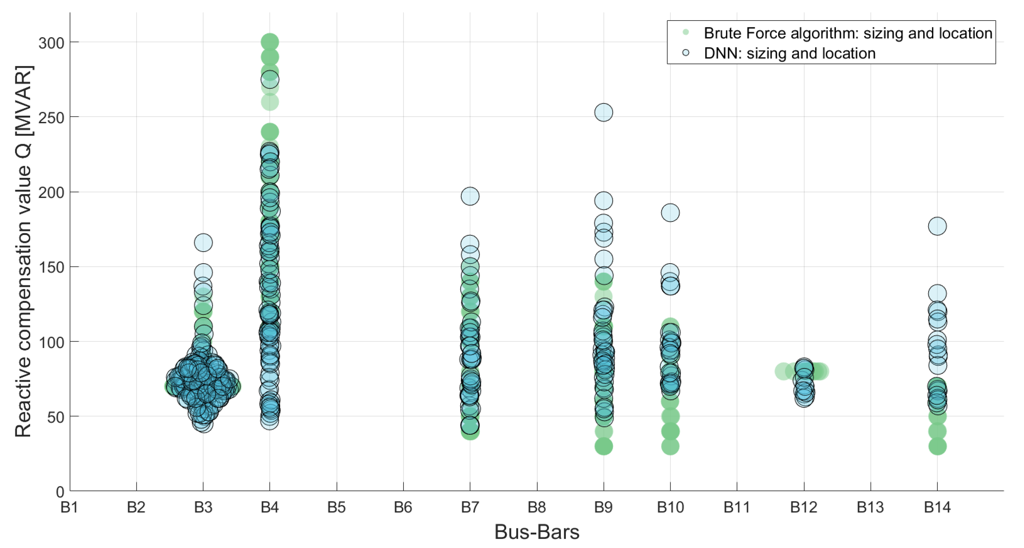
Afterwards, the DNN was trained by randomly selecting 70% of the input data and for validation, the other 30% was used as test data. By doing this, the test data allow the algorithm to verify the behaviour of the DNN results and to compare them with the brute force algorithm results, this analysis can be seen in Figure 3 for the test data (424 randomly selected cases).
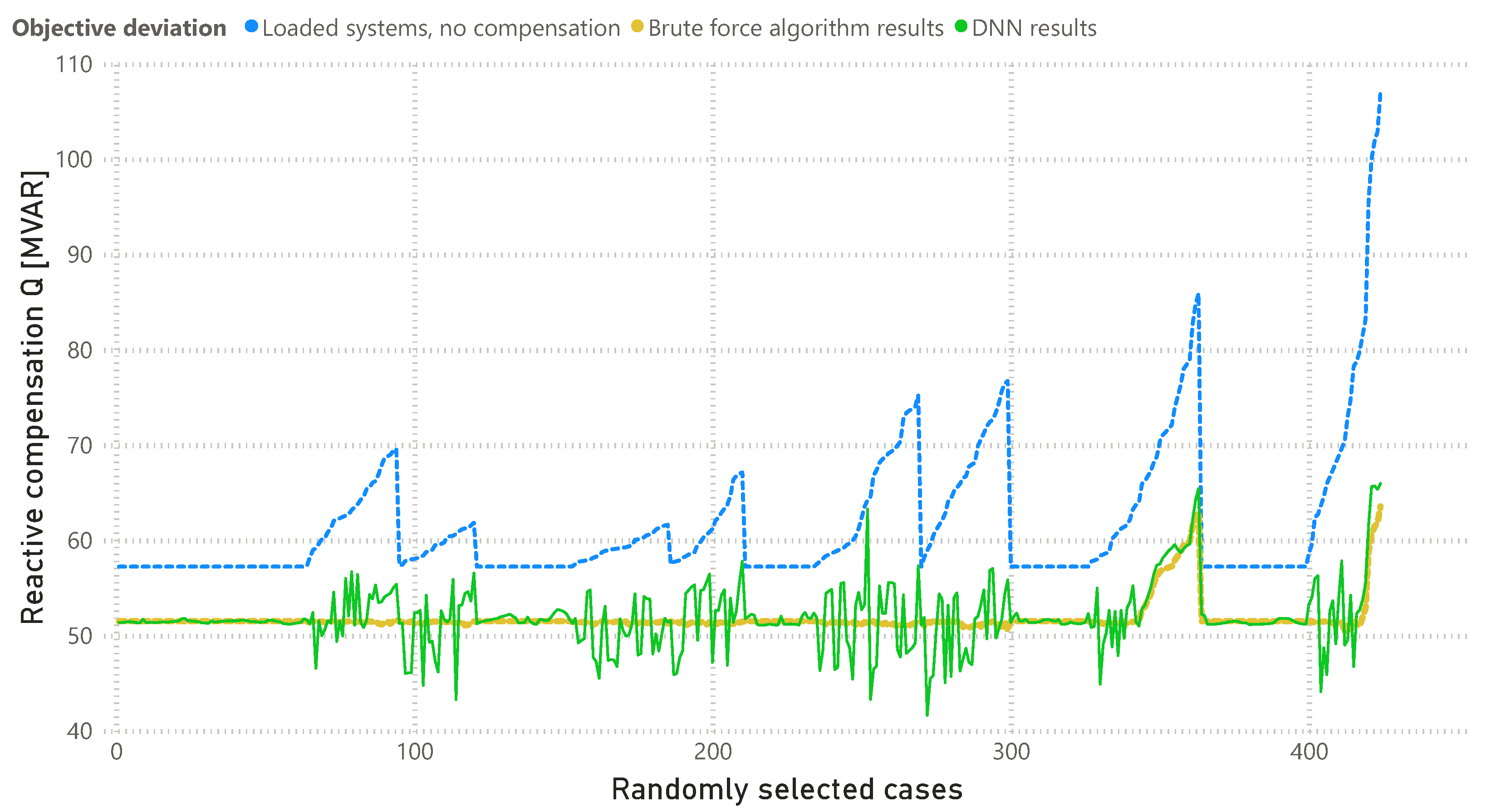
As can be seen in Figure 3, the x-axis shows the busbar location for reactive compensation and in both cases (the BFA and DNN) all compensation locations overlap, which indicates that DNN shows 100% accuracy for reactive compensation location (when compared with the BFA). For compensation sizing, the objective deviation for each scenario (424 test data scenarios) is calculated and a comparison between the results of objective deviation from the brute force algorithm, DNN and loaded system without compensation is shown in Figure 4. It should be noted that each objective deviation value is calculated following Equation (1), in other words, one point in every line represents the objective deviation of an IEEE 14 busbar system case of analysis.
Figure 4 shows that the main objective of this paper’s methodology is achieved because the DNN was capable of finding the optimal location and sizing for reactive compensation. Compensation location presents 100% accuracy and a comparison between the objective deviation for the brute force algorithm and the DNN when comparing all the test scenarios presents a difference of 3.18% (yellow and green lines in Figure 4).
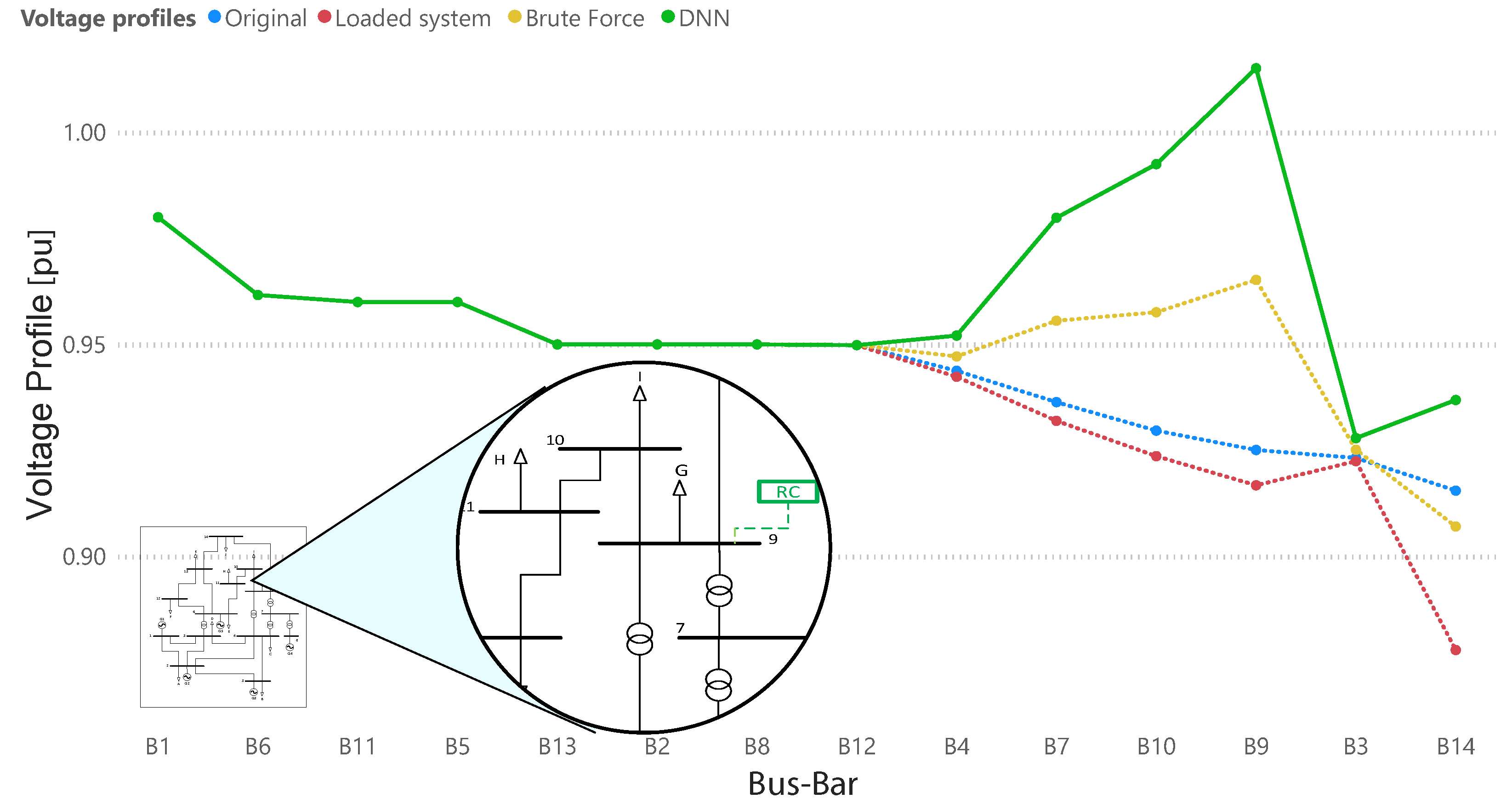
Additionally, one scenario where the objective deviation from BFA and DNN have similar values is shown in Figure 5. This figure shows the resulting voltage profiles after compensation, where, as it was proposed, the DNN improves the voltage profiles after a PQ load was connected to the system.
Figure 5 organizes voltage profiles from highest to lowest, by doing so the diagram is focused on the most affected busbars due to the connection of the additional load. In this particular scenario, a load of 100 MW–24 Mvar was connected to busbar 10 and the results from the DNN indicate that reactive compensation of 72 Mvar should be connected at busbar 10. This scenario affects specifically busbars 7, 10, 9 and 10, and after compensation was connected, all these affected busbars improved their voltage profiles and not only the busbar where compensation is connected, which in itself demonstrates this is an optimal solution.
Moreover, Figure 4 also shows scenarios where some results from the DNN have lower values (objective deviation) when compared with the brute force results; however, even in those cases, the resulting voltage profiles will achieve this research’s restrictions by been at least 90% higher than the original voltage profiles and no higher than the upper limit of 1.05 (p.u.). An example of this scenario is shown in Figure 6.
Figure 6 also organizes voltage profiles from highest to lowest. In this scenario, a load of 24 MW–6 Mvar was connected to busbar 14 and the results from the DNN indicate that reactive compensation of 107 Mvar should be connected at busbar 9.
This scenario specifically affects busbars 3, 9 and 14, and after compensation was connected all these affected busbars improved their voltage profiles. Improving not only the voltage profile at the busbar where compensation is connected demonstrates that the methodology finds an optimal solution.
Additionally, it is important to state that Figure 6 shows a scenario in which the reactive compensation sizing from the DNN is slightly greater than the results from the BFA for this reason voltage profiles of busbars 7, 9 and 10 are greater than the BFA ones; however, compensation locations are 100% accurate and the 1.05 p.u. upper limit for the voltage profile is not violated.
Finally, regarding processing time, BFA analyzes 30 permutations of reactive compensation in every busbar, then all cases are compared following limitations previously stated in Algorithms 1 and 2; thus a total of 420 scenarios are analyzed for each load added to the system. Every load flow is calculated in around 10 ms, which in total gives 4.2 s of processing time for a single scenario of added load. For the IEEE 14 busbar scenario, 1414 cases were analyzed and the total processing time for the BFA optimal values was 1.65 h. On the other hand, once the DNN was fully trained the processing time for all 1414 scenarios was 0.5 s.
3.2. Case Study: IEEE 30 Busbar System
Similarly to the previous case, when Algorithm 1 is applied to the IEEE 30 busbar system, a PQ load was connected to every busbar, with values from 1MW–0.25 Mvar to 100 MW–25 Mvar using steps of 1 MW. Algorithm 1 generates a matrix of 3030 rows and three columns where the first column is the active load power P, the second column is the reactive load power Q and the third column is the busbar in which the load was connected. This matrix is the input data for the deep neural network.
Then, Algorithm 2 is applied to all the scenarios generated with Algorithm 1. Algorithm 2 connected reactive compensation in every busbar, with values from 10 Mvar to 300 Mvar using steps of 10 Mvar, having 900 reactive compensation scenarios for every load added in Algorithm 1. Subsequently, the algorithm selects the optimal location and size for the reactive compensation. A matrix of 3030 rows and two columns is generated, where the first column is the compensation value and the second column is its busbar location. This matrix is the target data for the neural network.
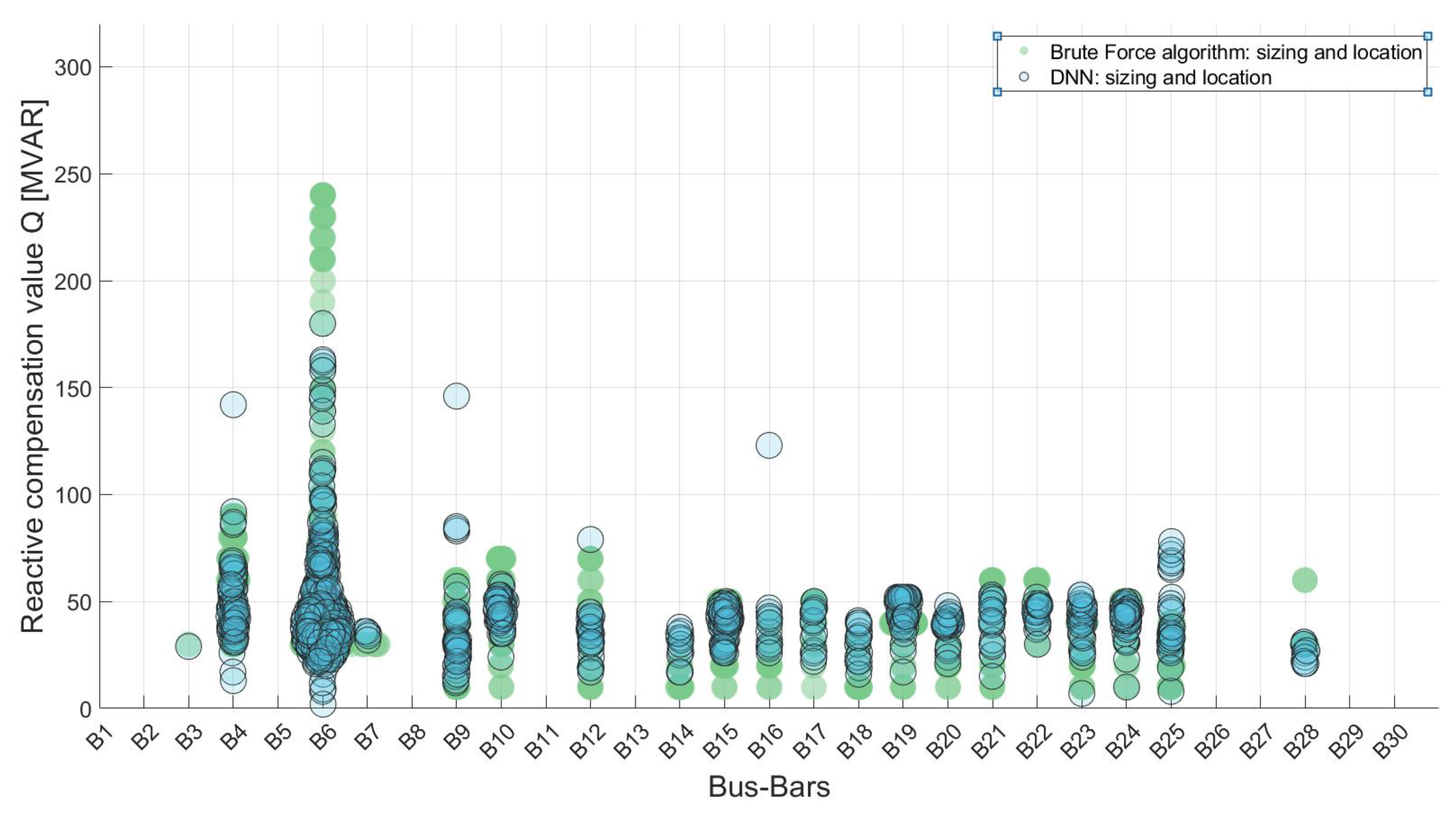
Afterwards, the DNN that was previously trained is also used for this case study. As for the IEEE 14 busbar system, 70% of the input data was selected randomly for validation, the other 30% was used as test data. Results for location and sizing between brute force and DNN are shown in Figure 7 for the test data (909 randomly selected cases).
As can be seen in Figure 7, the x-axis shows the busbar location for reactive compensation and in both cases (the BFA and DNN) all compensation locations overlap, which indicates that DNN shows 100% accuracy for reactive compensation location (when compared with the BFA). For compensation sizing, the objective deviation for each scenario (909 test data scenarios) is calculated and a comparison between the results of objective deviation from the brute force algorithm, DNN and loaded system without compensation is shown in Figure 8. It should be noted that each objective deviation value is calculated following Equation (1), in other words, one point in every line represents the objective deviation of an IEEE 30 busbar system case of analysis.
Figure 8 shows that the DNN is capable of finding the optimal location and sizing of reactive compensation in bigger transmission systems. Compensation location presents a 100% accuracy (when compared with the BFA) and a comparison between the objective deviation for the brute force algorithm and the DNN when comparing all the test scenarios presents a difference of 7.43% (yellow and green lines in Figure 8).
Additionally, taking as an example one scenario where the objective deviation from brute force algorithm and DNN have similar values, the resulting voltage profiles after compensation are shown in Figure 9, showing once again that the DNN achieves its objective.
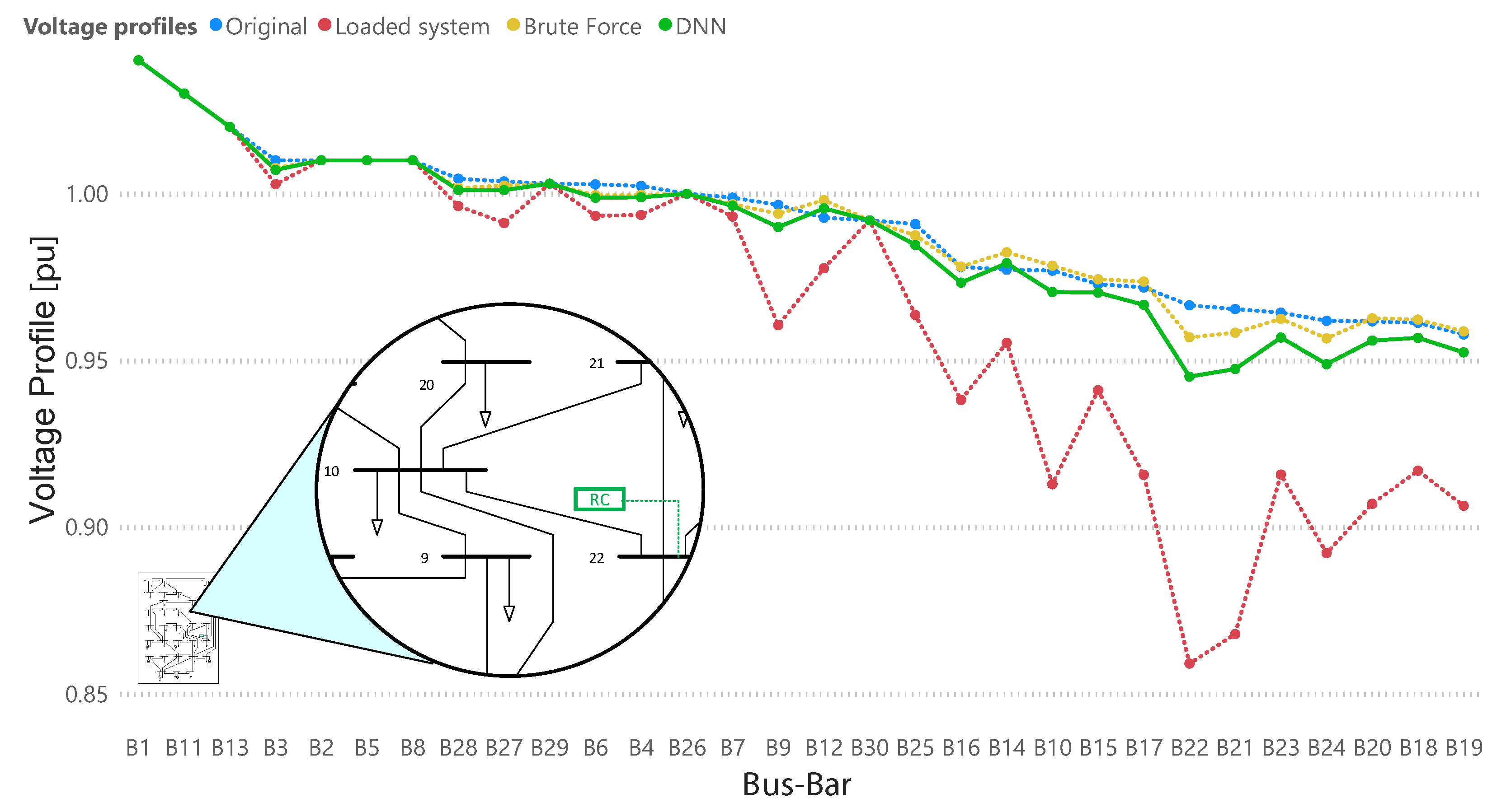
Figure 9 organizes voltage profiles from highest to lowest. In this scenario, a load of 100 MW–24 Mvar was connected to busbar 22 and the results from the DNN indicate that reactive compensation of 52 Mvar should be connected at busbar 22.
This scenario affects mainly busbars 10, 17, 21, 22 and 24, and after compensation was connected, all these affected busbars improved their voltage profiles and not only the busbar where compensation is connected, which in itself demonstrates this is an optimal solution.
Moreover, Figure 8 also shows scenarios where some results from the DNN have lower values (objective deviation) when compared with the brute force results, and as in the previous case study, even in those cases, the resulting voltage profiles will achieve this research’s restrictions by being at least 90% higher than the original voltage profiles and no higher than the upper limit of 1.05 (p.u.). An example of this scenario is shown in Figure 10.
Figure 10 also organizes voltage profiles from highest to lowest. In this scenario, a load of 76 MW–19 Mvar was connected to busbar 14 and the results from the DNN indicate that reactive compensation of 41 Mvar should be connected to busbar 15. This scenario affects mainly busbars 10, 14, 15, 16 and 17, and after compensation, connecting all these affected busbars improved their voltage profiles and not only the busbar where the compensation is connected, which in itself demonstrates that this is an optimal solution.
Finally, regarding processing time, the BFA analyzes 30 permutations of reactive compensation in every busbar, then all cases are compared following limitations previously stated in Algorithms 1 and 2; thus a total of 900 scenarios are analyzed for each load added to the system, every load flow is calculated in around 10 ms, which in total gives 9 s of processing time for a single scenario of added load. For the IEEE 30 busbar scenario, 3030 cases were analyzed and the total processing time for the BFA optimal values was 7.58 h. On the other hand, once the DNN was fully trained the processing time for all 3030 scenarios was 1.2 s.
3.3. Case Study: IEEE 118 Busbar System
Finally, the methodology was tested in the IEEE 118 busbar transmission system. When Algorithm 1 is applied to this system, a PQ load was connected to every busbar, with values from 1MW–0.25 Mvar to 100 MW–25 Mvar using steps of 1 MW. Algorithm 1 generates a matrix of 11918 rows and three columns, where the first column is the active load power P, the second column is the reactive load power Q and the third column is the busbar in which the load was connected. This matrix is the input data for the deep neural network.
Then, Algorithm 2 is applied to all the scenarios generated with Algorithm 1. Algorithm 2 connected reactive compensation in every busbar, with values from 10 Mvar to 300 Mvar using steps of 10 Mvar, having 3540 reactive compensation scenarios for every load added in Algorithm 1. Subsequently, the algorithm selects the optimal location and size for the reactive compensation. A matrix of 3540 rows and two columns is generated, where the first column is the compensation value and the second column is its busbar location. This matrix is the target data for the neural network.
Once again, the DNN was re-trained with this new data. A total of 70% of the input data was selected randomly for validation, the other 30% was used as test data. A total of 3575 scenarios of reactive compensation are analyzed, and the optimal location and sizing of reactive compensation for each one of these scenarios resulted in a 100% accuracy when compared with the results of the brute force algorithm (these results are not graphically shown due to their massive number).
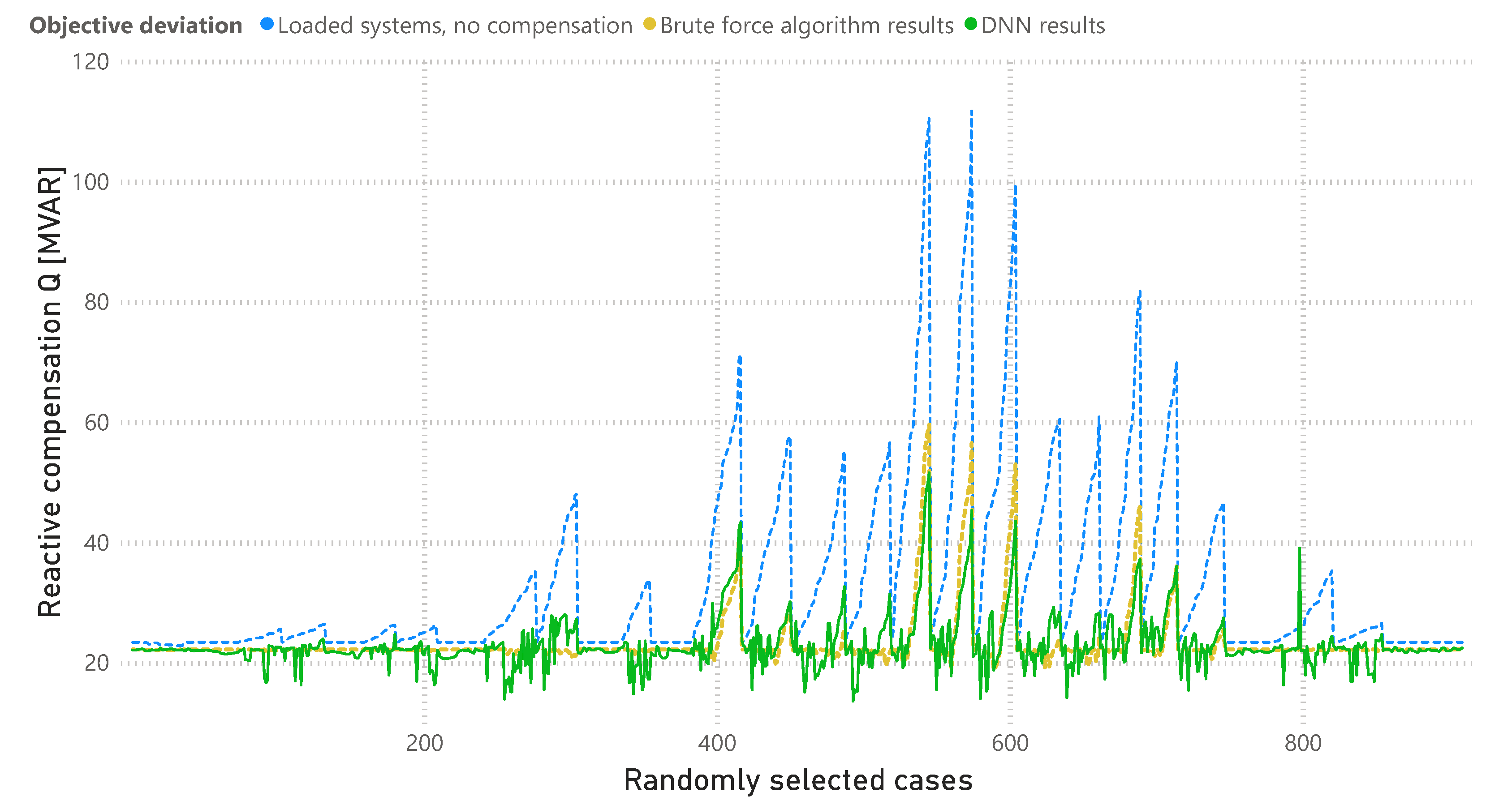
Then, for the 3575 scenarios objective, the deviation is calculated and a comparison between the results of objective deviation from the brute force algorithm, DNN and the loaded system without compensation is shown in Figure 11 (one of every five cases is shown due to the large amount of data). It should be noted that each objective deviation value is calculated following Equation (1). In other words, one point in every line represents the objective deviation of an IEEE 118 busbar system case of analysis.
Figure 11 shows that the objective deviation from the brute force algorithm and the DNN are the same (blue and green superposed lines), showing that due to further training the DNN has further improved, having a 100% accuracy for objective deviation (when compared with the BFA).
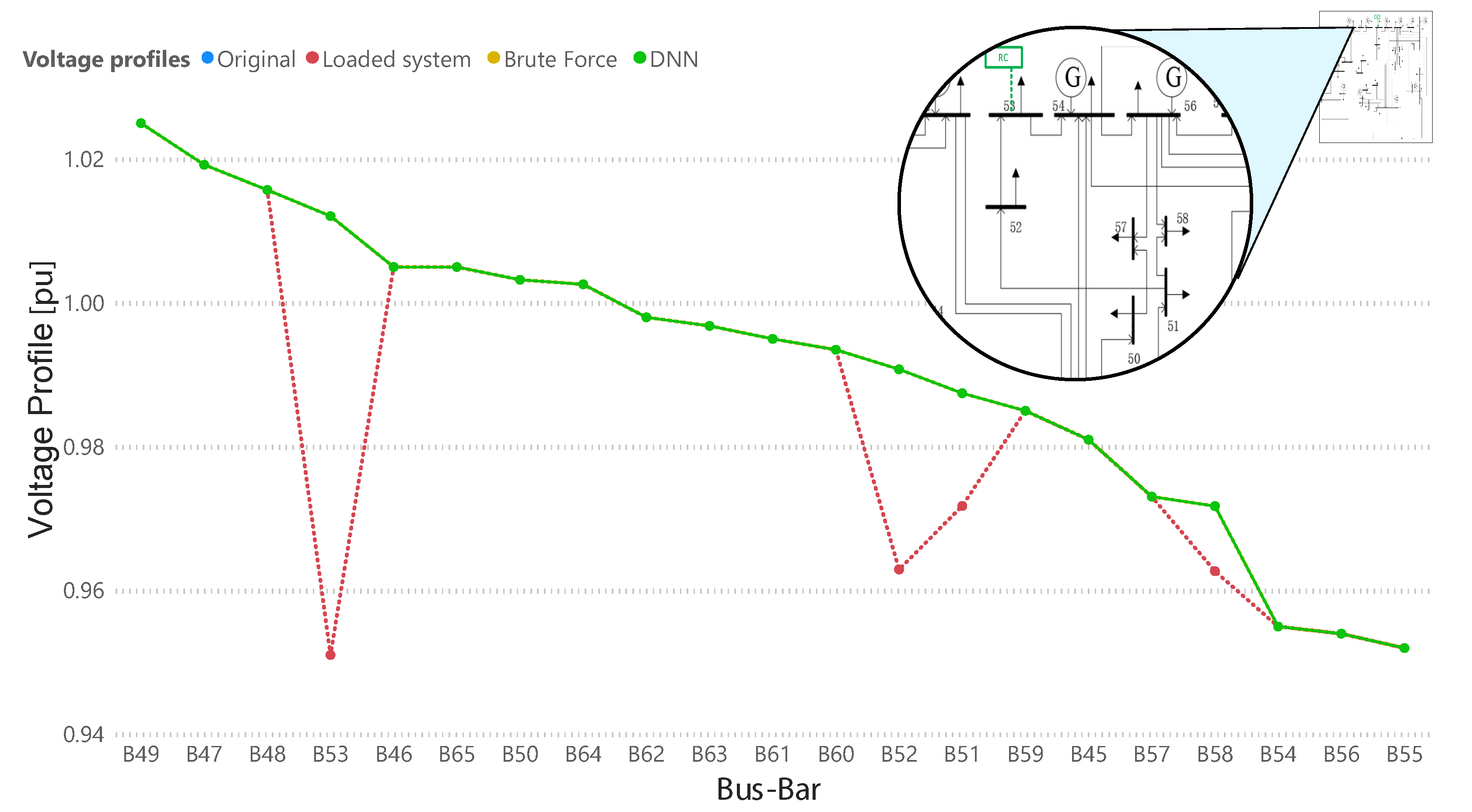
Moreover, taking as an example any scenario (all have 100% accuracy), the resulting voltage profiles for one compensation case are shown in Figure 12. Due to the large number of busbars, for this figure only the affected busbars (drop in voltage profiles) are displayed.
Figure 12 shows once again that the DNN achieves its objective and has further improved due to additional training. In these figures, once again it is shown that the optimal values for location and sizing of reactive compensation are the same as the ones from the DNN.
Figure 12 also organizes voltage profiles from highest to lowest. In this scenario, a load of 35 MW–8.75 Mvar was connected to busbar 73 and the results from the DNN indicate that reactive compensation of 70 Mvar should be connected at busbar 53. This scenario affects mainly busbars 51, 53, 53 and 58, and after compensation was connected, all these affected busbars improved their voltage profiles and not only the busbar where compensation is connected, which in itself demonstrates this is an optimal solution.
Finally, regarding processing time, the BFA analyzes 30 permutations of reactive compensation in every busbar, then all cases are compared following limitations previously stated in Algorithms 1 and 2; thus a total of 3540 scenarios are analyzed for each load added to the system, every load flow is calculated in around 10 milliseconds which in total gives 35.4 s of processing time for a single scenario of added load. For the IEEE 118 busbar scenario, 11,918 cases were analyzed and the total processing time for the BFA optimal values was 117.19 h. On the other hand, once the DNN was fully trained the processing time for all 11,918 scenarios was 5 s.
3.4. Results Summary
Table 3 shows a summary of results for optimal compensation and sizing of reactive compensation that this paper’s methodology achieved through deep neural networks. These results are compared with the results provided by the brute force algorithm.
4. Conclusions
Training is critical for the performance of a deep neural network, which is proved by this research when comparing this methodology’s performance for the IEEE 14, 30 and 118 busbar systems. The three study cases presented differences of 4.18%, 7.43% and 0% for reactive compensation sizing, respectively, when compared with a brute force algorithm. The third study case (IEEE 18 busbar system) had a 100% accuracy, which is an indicator of proper training and that sufficient data was taken for training (3540 scenarios were analyzed).
For the three study cases, the DNN achieved 100% accuracy for optimal reactive compensation location. On the other hand, for reactive compensation sizing, the IEEE 14 and 30 busbar systems had differences of 4.18% and 7.43%, respectively, when compared with a brute force algorithm. However, these differences do not indicate bad performance in compensation sizing, on the contrary, these differences indicate cases where the compensation was slightly over the result stated by the brute force technique. Nevertheless the DNN accomplished the restrictions established for this research (improved voltages profiles to at least 90%).
When compared with other methodologies such as optimization techniques or even the brute force algorithm that this paper itself uses for training the deep neural network, the biggest advantage of this work’s methodology is the processing speed that a computer takes to find the optimal solution for optimal location and sizing of reactive compensation under any random load addition scenario.
The DNN took 0.5 s to process and find the optimal solution for 1414 cases in the IEEE 14 busbar system, while the BFA took 1.65 h. For the IEEE 30 busbar, the DNN took 1.2 s to process 3030 cases while the BFA took 7.58 h. Finally, for the IEEE 118 busbar system the DNN took 5 s to process 11918 cases while the BFA took 117.19 h.
Author Contributions
M.J.: Conceptualisation, Methodology, Validation, Writing—review and editing, Data curation, Formal analysis. D.C.: Methodology, Validation, Writing—review and editing. J.M.: Writing—review and editing. All authors have read and agreed to the published version of the manuscript.
Funding
This work supported by Universidad Politécnica Salesiana and GIREI—Smart Grid Research Group under the project Forecast of electricity demand in the short and medium term using time series techniques and optimization heuristics.
Data Availability Statement
Not applicable.
Conflicts of Interest
The authors declare no conflict of interest.
Abbreviations
The following abbreviations are used in this manuscript:
| DNN | Deep neural network |
| BFA | Brute force algorithm |
| EPS | Electrical power system |
| PQ | Electrical load with active and reactive components |
| Objective deviation for voltage profiles | |
| Voltage profile in busbar i | |
| N | Number of busbars in a transmission system |
| NL | Number of layers of a deep neural network |
| Layer k of the deep neural network | |
| Number of neurons for layer k of the deep neural network | |
| PSO algorithm speed at time t | |
| PSO algorithm position at time t | |
| w | PSO algorithm inertia coefficient |
| PSO algorithm personal acceleration coefficient | |
| PSO algorithm social acceleration coefficient | |
| Particle i best position at time t in PSO | |
| Global best position at time t in PSO | |
| Decimal random value for updated local position in PSO algorithm | |
| Decimal random value for updated global position in PSO algorithm | |
| Integer random value for updated local position in PSO algorithm | |
| Integer random value for updated global position in PSO algorithm | |
| RSS | Residual sum of squares |
| Original electricity demand at position i | |
| Nbus | Number of busbars in an electrical power system |
| Impedance of line | |
| Active power load at node i | |
| Reactive power load at node i | |
| Max and min values of active power for generator at node i | |
| Max and min values of reactive power for generator at node i | |
| Max and min values of active power for generator at nodes | |
| Generation cost | |
| B | Susceptance |
| Voltage at node i | |
| Active power between nodes i and j | |
| Reactive power between nodes i and j | |
| Objective deviation of voltage profiles under normal conditions | |
| maxP | Maximum active power value for additional loads to be connected to the system |
| Variable for all combinations of electrical power systems with added loads | |
| Variable for all additional loads connected to the electrical power system | |
| maxComp | Maximum reactive compensation considered for this research |
| Variable for all scenarios of reactive compensations considered for each additional load connected to the electrical power system after power flow calculation | |
| Voltage profile at node i after power flow calculation | |
| Active power between nodes i and j after power flow calculations | |
| Reactive power between nodes i and j after power flow calculations | |
| Variable for all reactive compensations connected at the electrical power system | |
| Number of busbars at which compensation was connected | |
| Number of compensations at busbar | |
| OBJ | Objective deviation calculated for a compensated system |
| Index | Location of best scenario of objective deviation |
| Value of best objective deviation | |
| Value of best reactive compensation |
References
- Amroune, M. Machine Learning Techniques Applied to On-Line Voltage Stability Assessment: A Review. Arch. Comput. Methods Eng. 2021, 28, 273–287. [Google Scholar] [CrossRef]
- Tolba, M.A.; Zaki Diab, A.A.; Tulsky, V.N.; Abdelaziz, A.Y. VLCI approach for optimal capacitors allocation in distribution networks based on hybrid PSOGSA optimization algorithm. Neural Comput. Appl. 2019, 31, 3833–3850. [Google Scholar] [CrossRef]
- Ismail, B.; Abdul Wahab, N.I.; Othman, M.L.; Radzi, M.A.M.; Naidu Vijyakumar, K.; Mat Naain, M.N. A Comprehensive Review on Optimal Location and Sizing of Reactive Power Compensation Using Hybrid-Based Approaches for Power Loss Reduction, Voltage Stability Improvement, Voltage Profile Enhancement and Loadability Enhancement. IEEE Access 2020, 8, 222733–222765. [Google Scholar] [CrossRef]
- Tejaswini, V.; Susitra, D. Optimal Location and Compensation Using D-STATCOM: A Hybrid Hunting Algorithm. J. Control. Autom. Electr. Syst. 2021, 32, 1002–1023. [Google Scholar] [CrossRef]
- Alexander, A.T.; Gonzalo Manuel, G.S.; DIego Luis, G.S.; Leony, O.M. Optimum location and sizing of capacitor banks using VOLT VAR compensation in micro-grids. IEEE Lat. Am. Trans. 2020, 18, 465–472. [Google Scholar] [CrossRef]
- Gholami, K.; Karimi, S.; Dehnavi, E. Optimal unified power quality conditioner placement and sizing in distribution systems considering network reconfiguration. Int. J. Numer. Model. Electron. Netw. Devices Fields 2019, 32, e2467. [Google Scholar] [CrossRef] [Green Version]
- Montoya, O.D.; Chamorro, H.R.; Alvarado-Barrios, L.; Gil-González, W.; Orozco-Henao, C. Genetic-convex model for dynamic reactive power compensation in distribution networks using D-STATCOMs. Appl. Sci. 2021, 11, 3353. [Google Scholar] [CrossRef]
- Karmakar, N.; Bhattacharyya, B. Optimal reactive power planning in power transmission system considering facts devices and implementing hybrid optimisation approach. IET Gener. Transm. Distrib. 2020, 14, 6294–6305. [Google Scholar] [CrossRef]
- Al-Jubori, W.K.S.; Hussain, A.N. Optimum reactive power compensation for distribution system using dolphin algorithm considering different load models. Int. J. Electr. Comput. Eng. 2020, 10, 5032–5047. [Google Scholar] [CrossRef]
- Sanam, J. Optimization of planning cost of radial distribution networks at different loads with the optimal placement of distribution STATCOM using differential evolution algorithm. Soft Comput. 2020, 24, 13269–13284. [Google Scholar] [CrossRef]
- Gaddala, K.; Raju, P.S. Optimal location of UPQC for power quality improvement: Novel hybrid approach. J. Eng. Des. Technol. 2020, 18, 1519–1541. [Google Scholar] [CrossRef]
- Patil, B.; Karajgi, S. Simultaneous placement of facts devices using Cuckoo search algorithm. Int. J. Power Electron. Drive Syst. 2020, 11, 1344–1349. [Google Scholar] [CrossRef]
- Amini, M.; Jalilian, A. Optimal sizing and location of open-UPQC in distribution networks considering load growth. Int. J. Electr. Power Energy Syst. 2021, 130, 106893. [Google Scholar] [CrossRef]
- Jaramillo, M.; Tipán, L.; Muñoz, J. A novel methodology for optimal location of reactive compensation through deep neural networks. Heliyon 2022, 8, e11097. [Google Scholar] [CrossRef] [PubMed]
- Kirgizov, A.K.; Dmitriev, S.A.; Safaraliev, M.K.; Pavlyuchenko, D.A.; Ghulomzoda, A.H.; Ahyoev, J.S. Expert system application for reactive power compensation in isolated electric power systems. Int. J. Electr. Comput. Eng. 2021, 11, 3682–3691. [Google Scholar] [CrossRef]
- Frolov, V.; Thakurta, P.G.; Backhaus, S.; Bialek, J.; Chertkov, M. Operations- and uncertainty-aware installation of FACTS devices in a large transmission system. IEEE Trans. Control. Netw. Syst. 2019, 6, 961–970. [Google Scholar] [CrossRef] [Green Version]
- Belazzoug, M.; Chanane, A.; Sebaa, K. An efficient NSCE algorithm for multi-objective reactive power system compensation with UPFC. Indones. J. Electr. Eng. Comput. Sci. 2020, 22, 40–51. [Google Scholar] [CrossRef]
- Agha, A.; Attar, H.; Alfaoury, A.; Khosravi, M.R. Maximizing electrical power saving using capacitors optimal placement. Recent Adv. Electr. Electron. Eng. 2020, 13, 1041–1050. [Google Scholar] [CrossRef]
- Eltawil, N.; Sulaiman, M.; Shamshiri, M.; Bin Ibrahim, Z. Optimum allocation of capacitor and DG in MV distribution network using PSO and opendss. ARPN J. Eng. Appl. Sci. 2019, 14, 363–371. [Google Scholar]
- Nadeem, M.; Imran, K.; Khattak, A.; Ulasyar, A.; Pal, A.; Zeb, M.Z.; Khan, A.N.; Padhee, M. Optimal Placement, Sizing and Coordination of FACTS Devices in Transmission Network Using Whale Optimization Algorithm. Energies 2020, 13, 753. [Google Scholar] [CrossRef] [Green Version]
- Siddiqui, A.S.; Prashant. Optimal Location and Sizing of Conglomerate DG- FACTS using an Artificial Neural Network and Heuristic Probability Distribution Methodology for Modern Power System Operations. Prot. Control. Mod. Power Syst. 2022, 7, 9. [Google Scholar] [CrossRef]
- Chandrasekaran, K.; Selvaraj, J.; Xavier, F.J.; Kandasamy, P. Artificial neural network integrated with bio-inspired approach for optimal VAr management and voltage profile enhancement in grid system. Energy Sour. Part Recover. Util. Environ. Eff. 2021, 43, 2838–2859. [Google Scholar] [CrossRef]
- Li, C.; Coster, D.C. Article Improved Particle Swarm Optimization Algorithms for Optimal Designs with Various Decision Criteria. Mathematics 2022, 10, 2310. [Google Scholar] [CrossRef]
- Sengupta, S.; Basak, S.; Peters, R. Particle Swarm Optimization: A Survey of Historical and Recent Developments with Hybridization Perspectives. Mach. Learn. Knowl. Extr. 2018, 1, 157–191. [Google Scholar] [CrossRef] [Green Version]
- Rokbani, N.; Abraham, A.; Alimi, A.M. Fuzzy Ant supervised by PSO and simplified ant supervised PSO applied to TSP. In Proceedings of the 13th International Conference on Hybrid Intelligent Systems, HIS 2013, Gammarth, Tunisia, 4–6 December 2013; pp. 251–255. [Google Scholar] [CrossRef] [Green Version]
- Severino, A.G.V.; de Lima, J.M.M.; de Araújo, F.M.U. Industrial Soft Sensor Optimized by Improved PSO: A Deep Representation-Learning Approach. Sensors 2022, 22, 6887. [Google Scholar] [CrossRef]
Figure 1.
Deep neural network general topology example.

Figure 2.
Deep neural network topology applied in this research.

Figure 3.
Sizing and location results: DNN vs. brute force algorithm—IEEE 14 busbar.

Figure 4.
Objective deviations for 424 scenarios: original system, loaded system, brute force results and DNN results.
Figure 4.
Objective deviations for 424 scenarios: original system, loaded system, brute force results and DNN results.

Figure 5.
Voltage profiles for 14 bus-bar system: original system, loaded system, BFA and DNN compensation—BFA and DNN present similar results.
Figure 5.
Voltage profiles for 14 bus-bar system: original system, loaded system, BFA and DNN compensation—BFA and DNN present similar results.

Figure 6.
Voltage profiles for 14 bus-bar system: original system, loaded system, BFA and DNN compensation—where DNN results are better than BFA.
Figure 6.
Voltage profiles for 14 bus-bar system: original system, loaded system, BFA and DNN compensation—where DNN results are better than BFA.

Figure 7.
Sizing and location results: DNN vs. brute force algorithm—IEEE 30 busbar.

Figure 8.
Objective deviations for 909 scenarios: original system, loaded system, brute force results and DNN results.
Figure 8.
Objective deviations for 909 scenarios: original system, loaded system, brute force results and DNN results.

Figure 9.
Voltage profiles for 30 bus-bar system: original system, loaded system, BFA and DNN compensation—BFA and DNN present similar results.
Figure 9.
Voltage profiles for 30 bus-bar system: original system, loaded system, BFA and DNN compensation—BFA and DNN present similar results.

Figure 10.
Voltage profiles for 30 bus-bar system: original system, loaded system, BFA and DNN compensation—where DNN results are better than BFA.
Figure 10.
Voltage profiles for 30 bus-bar system: original system, loaded system, BFA and DNN compensation—where DNN results are better than BFA.

Figure 11.
Objective deviations for 3575: original system, loaded system, brute force results and DNN results.
Figure 11.
Objective deviations for 3575: original system, loaded system, brute force results and DNN results.

Figure 12.
Voltage profiles for 188 bus-bar system: original system, loaded system, brute force results and DNN results.
Figure 12.
Voltage profiles for 188 bus-bar system: original system, loaded system, brute force results and DNN results.


Table 1.
Most relevant results and methodologies for reactive compensation in the literature review.
Table 1.
Most relevant results and methodologies for reactive compensation in the literature review.
| Author | Year | Methodology | Test System | Parameters Considered | |||||
|---|---|---|---|---|---|---|---|---|---|
| Voltage Profile | Losses | Stability | Cost | Power Factor | THD | ||||
| Nadeem [20] | 2020 | Whale Optimization Algorithm | 14, 30 buses | ✓ | ✓ | - | - | - | - |
| Tejaswini [4] | 2021 | Hybrid heuristic: Prey Targeting Behavior of Whale and Grey Wolf Optimization | Distribution System | - | - | ✓ | - | - | - |
| Siddiqui [21] | 2022 | Probability-Based Heuristics with an Artificial Neural Network | 9, 57 Buses | - | ✓ | - | - | - | ✓ |
| Chandrasekaran [22] | 2021 | Artificial Neural Network Integrated with a Bio-Inspired Approach | 30 Buses | ✓ | ✓ | - | - | - | - |
| Gholami [6] | 2019 | Reconfiguration of the Distribution Network | 69 Buses | - | ✓ | - | - | - | - |
| Montoya [7] | 2021 | Genetic–Convex Method | 33 Buses | - | ✓ | - | ✓ | - | - |
| Karmakar [8] | 2020 | Probabilistic Hybridisation of Crow Search Algorithm and JAYA | 30, 75 Buses | - | ✓ | - | ✓ | - | - |
| Al-Jubori [9] | 2020 | Dolphin algorithm | 16, 33 Buses | ✓ | ✓ | - | ✓ | - | - |
| Kirgizov [15] | 2021 | Fuzzy Logic and Bio-Genetic Algorithms | 46 Buses | ✓ | ✓ | - | - | ✓ | - |
| Alexander [5] | 2020 | Particle Swarm Optimization | Micro-grid | ✓ | ✓ | - | - | ✓ | - |
| Present Work | Depp Neural Network and Particle Swarm Optimization | IEEE 14, 30 and 118 Buses | ✓ | - | - | ✓ | - | - | |
Table 2.
Maximum load restrictions for study cases in the IEEE 14, 30 and 118 busbar systems.
| Parameters | IEEE Test System: Case of Study | ||
|---|---|---|---|
| 14 Busbar | 30 Busbar | 118 Busbar | |
| Highest Load | 94 MW | 94 MW | 130 MW |
| Location | B3 | B5 | B80 |
| Maximum load increment before instability | 220% of the maximum load | 190% of the maximum load | 180% of the maximum load |
Table 3.
Results comparison between the DNN and BFA for all study cases.
| BFA Algorithm | DNN’s Data Cases | DNN Performance (Compared with BFA) | Processing Time | ||||
|---|---|---|---|---|---|---|---|
| Study Case | Number of Scenarios Analized | Training Scenarios (70%) | Validation Scenarios (30%) | For Location | For Sizing | BFA (Hours) | DNN (Seconds) |
| IEEE 14 busbar | 1414 | 989 | 425 | 100% accurate | 4.18% difference | 1.65 | 0.5 |
| IEEE 30 busbar | 3030 | 2121 | 909 | 100% accurate | 7.43% difference | 7.58 | 1.2 |
| IEEE 118 busbar | 11,918 | 8342 | 3576 | 100% accurate | 0% difference | 117.19 | 5 |
Publisher’s Note: MDPI stays neutral with regard to jurisdictional claims in published maps and institutional affiliations. |
© 2022 by the authors. Licensee MDPI, Basel, Switzerland. This article is an open access article distributed under the terms and conditions of the Creative Commons Attribution (CC BY) license (https://creativecommons.org/licenses/by/4.0/).
Share and Cite
MDPI and ACS Style
Jaramillo, M.; Carrión, D.; Muñoz, J. A Deep Neural Network as a Strategy for Optimal Sizing and Location of Reactive Compensation Considering Power Consumption Uncertainties. Energies 2022, 15, 9367. https://doi.org/10.3390/en15249367
AMA Style
Jaramillo M, Carrión D, Muñoz J. A Deep Neural Network as a Strategy for Optimal Sizing and Location of Reactive Compensation Considering Power Consumption Uncertainties. Energies. 2022; 15(24):9367. https://doi.org/10.3390/en15249367
Chicago/Turabian StyleJaramillo, Manuel, Diego Carrión, and Jorge Muñoz. 2022. "A Deep Neural Network as a Strategy for Optimal Sizing and Location of Reactive Compensation Considering Power Consumption Uncertainties" Energies 15, no. 24: 9367. https://doi.org/10.3390/en15249367
Note that from the first issue of 2016, this journal uses article numbers instead of page numbers. See further details here.