Impact of Renewable Energy Sources and Nuclear Energy on CO₂ Emissions Reductions—The Case of the EU Countries

Abstract

The aim of this work is to analyse the dependence of carbon dioxide (CO₂) emissions on total energy consumption, the energy produced from renewable sources, the energy produced in nuclear power plants and the gross domestic product (GDP) in 22 European countries, over the period 1992–2019. The fully modified ordinary least squares model (FMOLS) and dynamic OLS (DOLS) were used to estimate the long-term cointegration relationship between the variables. First differenced (FD) general moments methods (GMM) were used in the estimation of short-run relationship dynamics. The results suggest that energy produced from renewable sources causes a reduction in CO₂ emissions per capita. On the other hand, total energy consumption increases CO₂ emissions in the long run. Although the mitigation effect of nuclear power was not found to be significant across the entire block of countries studied, a closer look at countries utilising nuclear energy reveals that nuclear energy positively affects the reduction in CO₂ emissions. Economic growth also has a positive effect on the reduction in CO₂ emissions, which confirms the decoupling of economic development from environmental impacts. These findings are crucial for understanding the causality between these variables and the adoption of new or revision of existing policies and strategies promoting the carbon-neutral and green economy at the EU and national level.

1. Introduction

Energy has been an integral part of the European Union since the earliest stages of its creation, starting with the European Coal and Steel Community (1951) and later EURATOM (in 1957) through the Single European Act and the Single Market Program. The main priorities in this area have evolved and shifted over time, from ensuring energy security and reducing energy dependency through forming the internal energy market, to the present day, where energy-related issues are closely linked to the climate agenda [1]. Linking the energy and climate agendas is based on the evidence of a number of studies as well as comprehensive research by the Intergovernmental Panel on Climate Change (IPCC) climatologists, who warn that if CO₂ emissions do not peak in 2025 and halve in the next decade, achieving a temperature rise of 1.5 °C (compared to pre-industrial levels) by the end of the millennium we will be in jeopardy. If no mitigating action is taken, the effects of warming will be further aggravated, some of which will be irreversible [2,3,4].

Concerns about the negative impacts of climate change have been reflected in international strategic documents such as the Kyoto Protocol and the current Paris Agreement, which have been accepted by a majority of world leaders as an expression of commitment to a global initiative to reduce CO₂ emissions. It was the adoption of the Paris Agreement that encouraged the EU to rethink its goals of decarbonising the economy and energy transition [5]. The European Green Deal, adopted in 2019, presented the Union’s ambition to become the first carbon-neutral continent by 2050 and declared climate action as the top priority. In June 2021, the EU adopted the European Climate Law. The document makes both the new targets and the goal of reaching climate neutrality by 2050 binding for all member states. In addition, a month later, the European Commission presented “Fit for 55”—a package of legislative proposals which aims to modernise climate and energy policy and introduce new measures to enhance transformational changes in society, economy and industry aimed at achieving climate neutrality targets.

Although overall greenhouse gas emissions in Europe have been declining over the last three decades [6], energy production and consumption remain the leading producers of carbon emissions. They are therefore seen as cornerstones of climate change mitigation and achieving the ambitious net carbon neutrality targets that the EU has committed to reaching by the middle of the century.

Reducing the carbon intensity of the energy sector is possible through a combination of measures, focused on increasing energy efficiency and boosting the use of renewable and low-carbon energy sources. To capture the untapped potential of energy efficiency, the European Commission has taken a number of measures, in particular in the residential sector [7]. Another strand of measures aims at increasing the share of renewables such as wind, water, solar and geothermal energy. It consists of investments in new and existing technologies as well as the creation of an efficient energy system ensuring the supply of large shares of renewable energy to the final consumer [8]. However, efforts to decarbonise economies are also associated with the possibility of higher use of so-called low-carbon sources, including nuclear energy. Here, however, the views of the professional community differ significantly. Some authors consider this resource as sustainable and inevitable for achieving decarbonization targets [9,10], while others point to the limitations of the technology [11] and the need to perceive technology throughout the life cycle lenses [12], pointing to the carbon footprint associated with power plant construction, as well as the problem of nuclear waste and the risks of its proliferation [13,14].

In light of decarbonisation efforts and the fulfilment of ambitious EU goals in the area of carbon neutrality, it is therefore very important to understand the role of RES and nuclear energy in reducing greenhouse gas emissions. This study analyses the long-term and short-term relationship between economic growth, energy consumption, energy consumption from low-carbon sources and CO₂ emissions. Even though nuclear energy is among the controversial energy sources and the views of the public, politicians and experts on nuclear energy are largely critical, the position of this energy source plays an important role in achieving the goals of carbon neutrality and energy security of many European countries. This study therefore also focuses on the importance of this energy source and its contribution to the decarbonisation of the energy sector within individual countries and the EU as a whole.

The paper is organised as follows: an overview of the related literature is presented in Section 2. The materials and methods are described in the Section 3, followed by a presentation of the results and their discussion. The last part concludes the paper.

2. Literature Review

The challenges of climate change, energy resource limitations and sustainable economic development have sparked the interest of the professional community in exploring the nexus between economic growth, energy consumption and greenhouse gas emissions. The relationship between economic, energy and environmental variables is well-known and extensively documented in the literature [15,16,17,18,19]. Some studies use single-country cases to assess the relationships between these variables. For example, Ang [20] explores the dynamic relationship between energy consumption, economic output and CO₂ emissions in France. Empirical results over the period 1960–2000 suggest a positive impact of economic growth on CO₂ and energy consumption in the long run and the short-run causality running from growth of energy use to economic growth.

Zhang and Cheng focus their scientific interest on the economy–energy–emissions nexus in China. Analysis of data from 1960–2007 suggests a unidirectional Granger causality running from economic output to energy consumption, and a long-run unidirectional causality running from energy use to CO₂ [21]. A more recent study concerning China confirms the existence of long-term equilibrium between the examined variables. The findings indicate that energy consumption positively impacts economic growth. However, CO₂ emissions are positively related to economic slowdown. The author of the study highlights the importance of environmental regulation, and how it boosts the economy, although the results are visible only in the long run [22]. However, in another study examining the relationship between economic growth, energy consumption and CO₂ emissions in China, the variables urbanisation and international trade are included in the model. The results indicated that economic growth, energy consumption and international trade significantly contribute to the increase in CO₂ emissions, while urbanisation reduces CO₂ emissions in the long run [23].

Many studies addressing the energy–economy–environment nexus provide a multi-country or regional perspective. The Middle East and North Africa (MENA) countries were investigated by Farhani and Shahbaz [24]. The results of their analysis confirm the environmental Kuznets curve hypothesis in the relationship between economic growth and CO₂ emissions. Panel data analysis revealed short-run causality running from electricity consumption (both renewable and non-renewable) and output to CO₂ emissions. Bidirectional causality between electricity consumption and CO₂ emissions is present in the long run. Similarly, Gorus and Aydin [25] found a unidirectional relationship running from energy consumption to CO₂ in the short-run in the MENA region. However, the study does not confirm the nexus between economic growth and carbon emissions, implying that conservation energy policies do not negatively impact the economy of the MENA countries, both in the long and short run.

More recently, Mensah et al. [26] analysed 22 African countries, both oil and non-oil exporters. They found bidirectional causality between energy consumption and economic growth and energy consumption and carbon emissions. The results differ for both groups: in the case of oil-exporting countries, the relationship between economic growth and emissions is confirmed in the long run. However, the unidirectional relationship running from energy consumption to economic growth has been confirmed in the case of non-oil exporters in a long- and short-term perspective.

The factors influencing carbon emissions were investigated in a study by Ahmed et al. [27]. The results of a panel data analysis of five South Asian economies suggested that energy consumption, trade openness and population growth have a positive effect on carbon emissions, which means that they cause an increase in CO₂ emissions.

Many studies employ the environmental Kuznets curve (EKC) to explore the relationship between economic growth, energy consumption and environmental impacts. E.g., Pao and Tsai [28] focused on the trio nexus in BRIC (Brazil, Russia, India and China) countries. The study indicates the long-run bidirectional causality between energy consumption and CO₂ emissions as well as energy consumption and economic output. Similarly, three regions consisting of 48 countries were analysed in a study by Kais and Sami [29]. The positive impact of energy use on CO₂ emissions was confirmed for all the panels. In both studies, the relationship between GDP per capita and CO₂ emissions confirms the validity of the EKC hypothesis.

Empirical evidence supports the positive impact of renewables at the energy–economy–environment nexus. Economic growth contributes to environmental pollution and renewable energy use. Renewables are, in turn, considered a mitigating factor in reducing greenhouse gas emissions [30,31,32] and also contribute to economic growth [33,34]. For example, Cheng and Liu [35] analysed the effect of energy consumption from different sources on economic growth in China. Their findings indicate that in terms of multiplying effect, clean energy (i.e., hydro, nuclear, wind and solar) has the highest contribution rate to economic growth.

The effect of non-renewable and renewable energy use on CO₂ emissions was also investigated for OECD countries [36]. The study in question provides evidence of the boosting effect of non-renewable resources and the mitigating effect of renewables on CO₂ emission levels. Mixed results were obtained in the study by Anwar et al. [37], who employed data from 59 countries divided into different income groups. The results vary among the studied panel countries. However, they conclude that a higher share of nuclear energy leads to a reduction in CO₂ emissions, except for the panel of upper–middle-income countries.

However, Charfeddine and Kahia [38] scrutinised the role of renewable energy consumption in MENA countries. The results of the panel data analysis suggest only a slight influence of renewables consumption and financial development on CO₂ emissions and economic growth. Based on the outputs of the analysis, the authors present policy recommendations for enhancing economic development and improving environmental quality in the region.

Several studies also focus on the energy–economy–emissions nexus in EU countries [39,40,41,42]. For example, the study by Menegaki [43] of 27 EU countries confirmed the neutrality hypothesis, suggesting that renewables do not play a significant role in GDP growth in Europe over the period 1997–2007. However, short-term causality was found between renewables, greenhouse gas emissions and employment. More recently, Radmehr et al. [44] have analysed the nexus between renewable energy consumption, CO₂ emissions and economic growth in the EU countries in the period 1995–2014. They found a feedback relation between economic growth and carbon emissions, and between economic growth and renewable energy consumption. The findings also provide evidence of the unidirectional relationship between renewable energy and CO₂ emissions, implying that a higher share of renewables in the energy mix is associated with a decrease in CO₂ emissions.

Similarly, Petruška et al. [18] analysed the dependence of CO₂ emissions on primary energy consumption at different GDP levels in 28 EU countries, including Great Britain. The study revealed that with increasing GDP levels, the regression coefficient of the dependence of CO₂ emissions on energy consumption decreases.

Several studies scrutinising the role of nuclear energy in the energy–economy–emissions nexus can be found in the literature. Nuclear energy–economic growth in 13 OECD countries was examined by Ozcan and Ari [45]. Their findings support the feedback hypothesis, i.e., nuclear energy consumption and economic growth influence and complement each other, both in the short run and long run. Moreover, in 6 out of 13 countries, nuclear energy positively and significantly impacted the real GDP in the long run. This analysis was complemented by Gozgor et al. [46], who provided evidence that both non-renewable and renewable energy consumption in OECD countries is positively associated with a higher rate of economic growth. Al-Mulali et al. [47] performed an analysis of disaggregated renewable electricity production by the source of CO₂ emissions in 23 EU member states. According to the results of the analysis, combustible renewables and waste, hydro energy and nuclear energy have a negative effect on CO₂ emissions, while the effect of solar and wind power is insignificant in the long run. Taking into account the other variables, the study suggests that GDP growth, urbanisation and financial development contribute to CO₂ increase, while trade openness reduces it in the long run.

Despite the plethora of studies examining the energy–economy–environment nexus, this study has a clear rationale and novelty: (1) the inclusion of the variables nuclear and renewable energy sources is especially vital as EU countries need to address both the problem of decarbonising the economy and at the same time reducing their energy dependence on fossil fuels imported from third countries. (2) The analysis employs current and robust estimation techniques, including fully modified OLS (FMOLS) and dynamic OLS (DOLS) to estimate long-run cointegration relationships; the panel VAR model and general moment model (GMM) were deployed for short-run dynamics estimation and finally, impulse response function was used to trace the reaction of a model’s variables to a shock in one or more variables. (3) The study fills a knowledge gap on the role of renewables and nuclear energy in climate change mitigation and decarbonisation of energy systems. Given the changing conditions of an exogenous nature, such as the COVID-19 pandemic and the war in Ukraine, an analysis of the evolution of these factors is essential when deciding on a modification or thorough revision of energy and climate policies. The study also reflects the 2030 Agenda and its Sustainable Development Goals, in particular SDG 7 on affordable and clean energy, SDG 12 on responsible production and consumption and SDG 13 on climate action.

3. Materials and Methods

3.1. Data Sources and Description of Variables

This study analyses the effect of energy consumption, renewable energy consumption, nuclear energy consumption and gross domestic product on CO₂ emissions. Renewable energy sources include wind energy, solar energy, hydro energy, geothermal energy and biomass. Data from 22 European countries from 1992 to 2019 were used for the analysis. The countries are as follows: Austria (AUT), Belgium (BEL), Bulgaria (BGR), Czech Republic (CZE), Denmark (DNK), Finland (FIN), France (FRA), Germany (DEU), Greece (GRC), Hungary (HUN), Ireland (IRL), Italy (ITA), Luxembourg (LUX), Netherlands (NLD), Poland (POL), Slovenia (SVN), Slovak Republic (SVK), Spain (ESP), Romania (ROU), Portugal (PRT), Sweden (SWE) and United Kingdom (GBR). The relationships between the five variables were examined. The list of investigated variables along with their abbreviated names used in the analyses is as follows:

• Carbon dioxide (CO₂) emissions per capita (tons)—CO₂;
• Gross domestic product (GDP) per capita (thousands USD)—GDP;
• Total energy consumption per capita (MWh)—TEC;
• Energy produced from renewable sources per capita (MWh)—RES;
• Energy produced in nuclear power plants per capita (MWh)—Nuclear.

3.2. Descriptive Statistics

The main focus of the study was analysing the effect of economic variables (GDP per capita) and energy variables (total energy consumption per capita, renewable energy per capita and nuclear energy per capita) on the carbon dioxide (CO₂) emissions per capita. The dependence of carbon dioxide (CO₂) emissions per capita on other variables was investigated in a multidimensional context. Summarised descriptive statistics are presented in

Table 1. Descriptive statistics of investigated variables.

Variable	Unit	Mean	Std. Dev	Min	Max
CO2	tons	8.784	3.721	3.818	31.253
GDP	thousands USD	30.406	17.058	4.504	124.591
TEC	MWh	44.345	17.233	17.920	114.632
RES	MWh	4.259	5.394	0.055	26.539
Nuclear	MWh	4.637	5.726	0	23.385

.

3.3. Empirical Methodology

Data that are repeated T times at regular time intervals from N statistical units (individuals, regions, countries, etc.) are well-known as panel data. Panel data properties are a combination of properties of cross-sectional data and time series. Their values are often denoted Y_it, where the i subscript, i = 1, 2, …, N, denotes the cross-section dimension, whereas the t subscript, t = 1, 2, …, T denotes the time-series dimension [48].

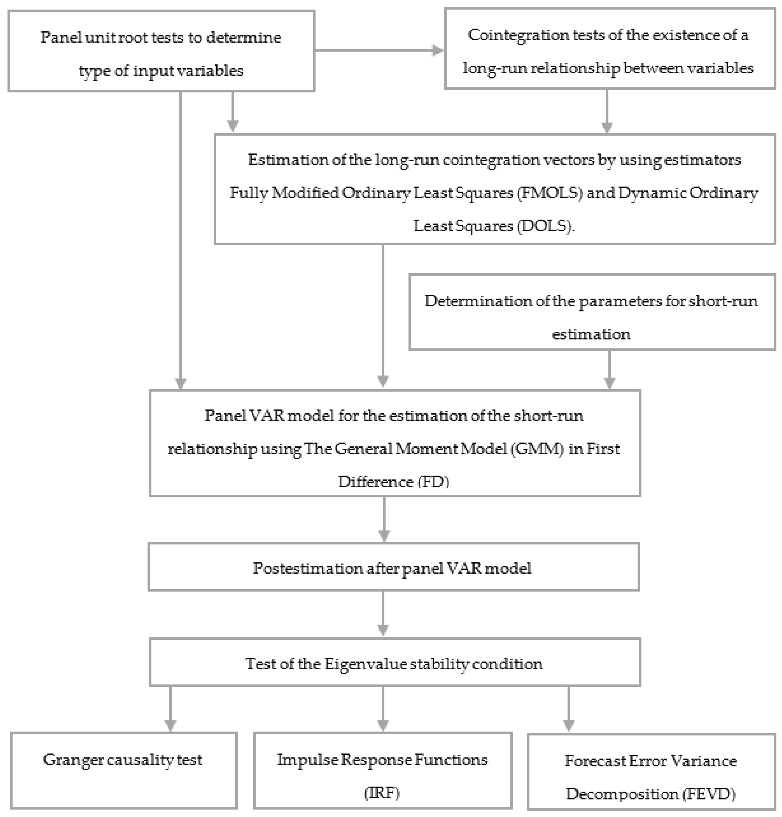
In this study, we use panel cointegration analysis and longitudinal dynamic estimation to analyse the relationship between CO₂ emissions, gross domestic product, energy consumption, renewable energy consumption and nuclear energy consumption on panel data of 22 countries for 28 years. In the short run, we use panel vector autoregression (PVAR) and the subsequent Granger causality test estimation. We used the impulse response function (IRF) and forecast error variance decomposition (FEVD) methods to evaluate the VAR output.

For better clarity, the methodological apparatus is captured in the process flowchart in Figure 1.

As a first step, before applying these methods, it is necessary to check whether the series in all panels are covariance stationary or whether their autoregressive representation contains one or more unit roots. The order of integration of the series under consideration is determined using panel root tests. The first such tests were used in the 1990s. Currently, we distinguish between first- and second-generation panel unit root tests. The main difference between the generations of unit root tests is that the first generation assumes that the individual time series in the panel were cross-sectionally independent, while the second generation finds ways to account for cross-sectional dependence [49]. Different norm definitions for different types of cross-sectional dependence were proposed by [50]. As for the tests of first-generation roots, we apply Harris and Tzavalis [51], Breitung [52]; Breitung and Das [53], Levin et al. [54], Im et al. [55] and Fisher type [56] tests, which have as null hypothesis that all panels contain a unit root, and Hadri’s [57] test, which in turn has as null hypothesis that all panels are stationary. Almost all of these tests assume strongly balanced panel data, and several of them have the limitation of assuming that all panels have the same autoregressive parameter in the autoregressive model being tested. In this study, we used one of the second-generation tests, namely Pesaran’s CIPS test [49,58], with tabulated critical values following Pesaran [49].

The second step is to establish the existence of a cointegrating relationship between the variables under analysis. The evolution of economic time series, whose correlation is justified by some economic theories, does not diverge over time. After short-term fluctuations, the system returns to equilibrium. Statisticians refer to this state as cointegration. Cointegration tests are used to determine whether there is a long-run stable relationship between variables. In the second step, we used Kao [59], Pedroni [60,61] and Westerlund [62] cointegration tests on a panel data set.

After demonstrating the existence of cointegration, a long-term dynamic estimate was made in the panels using two consistent estimates, FMOLS (fully modified ordinary least squares) [63] and DOLS (dynamic ordinary least squares) [64,65], proposed in the panel data by Phillips and Moon [66], Kao and Chiang [67] and Pedroni [68]. According to Pedroni [69], the FMOLS estimator has the ability to consider heterogeneity between panel units and can control for the bias induced by the potential endogeneity of regressors, and the serial correlation and heteroskedasticity of residuals [58].

In the third step, we used the panel vector autoregression (PVAR) model [70] following [71] and the Granger causality test [72] to analyse the relationship between CO₂ emissions, gross domestic product, energy consumption, renewable energy consumption and nuclear energy consumption in the short run. The coefficients of the PVAR model were estimated using general moment methods (GMMs) within a first difference (FD) model.

The k-variate homogeneous panel VAR of order p with panel-specific fixed effects takes the following form of a system of linear equations:

$$\begin{gathered} Y_{it}={\displaystyle \sum }_{j=1}^p{Y}_{it-j}{A}_j+X_{it}B+u_i+e_{it} \\ i\in \left\{1,2, \dots ,N\right\}, t\in \left\{1,2, \dots ,T\right\} \end{gathered}$$

(1)

where Y_it = (Log_CO_{2 it}, Log_GDP_it, Log_TEC_it, Log_RES_it, Nuclear_it) is a vector of k = 5 endogenous dependent variables, X_it is a (1 × l) vector of l exogenous covariates and the terms u_i and e_it are (1 × k) vectors of dependent variable-specific panel fixed effects and idiosyncratic errors. The (k × k) matrices A_j for j = 1, 2, …, p and the (l × k) matrix B are parameters to be estimated, and e_it are mutually independent with zero mean and constant variance. PVAR combines features of panel models and VAR models while systematic cross-sectional heterogeneity is modelled as panel-specific fixed effects.

For the same reasons, we use the PVAR model as described in [38], including: (I) the possibility of evaluating the reaction of our investigated variable, i.e., CO₂ emissions, to a one standard deviation shock on all the explanatory variables; (II) the ability to evaluate the contribution of all the variables of the system to the variability in CO₂ emissions by using forecast error variance decomposition (FEVD); and (III) the PVAR model allows the analysis of the causality direction between all the models under the study framework.

To solve Equation (1), we use the general moment model (GMM) in the first difference (FD). The GMM estimator of the above equation proposed by Hansen [73] is consistent when its two assumptions are met. This estimator includes the weighting matrix assumed to be non-singular, symmetric and positive semidefinite, which may be selected to maximise efficiency [71]. The order of the PVAR model was estimated using the [73] J statistic of over-identifying restriction and commonly used maximum likelihood-based model-selection criteria, the Akaike information criteria (AIC) [74], the Bayesian information criteria (BIC) [75,76,77] and the Hannan–Quinn information criteria (HQIC) [78]. The optimal lag order p and moment condition q are chosen through MMSC [79] for the GMM estimator based on Hansen’s J statistic of over-identifying restriction [73]. This is a selection of a pair of model and moment selection vectors (p, q) that minimise:

MMSC_BIC,n (k, p, q) = J_n (k²p, k²q) − (|q| − |p|) k² ln n

MMSC_AIC,n (k, p, q) = J_n (k²p, k²q) − 2k² (|q| − |p|)

MMSC_HQIC,n (k, p, q) = J_n (k²p, k²q) − Rk (|q| − |p|) ln ln n R > 2

where J_n (k, p, q) is Hansen’s statistic of over-identifying restriction for a k-variate panel VAR model of order p and moment conditions based on q lags of the dependent variable with sample size n. The overall coefficient of determination CD can be used as an alternative criterion [71].

In the last, fourth step, the analysis of the results was performed using the impulse response functions (IRF) and forecast error variance decomposition (FEVD) methods.

An important prerequisite for the implementation of the PVAR model is the eigenvalue stability condition. Lütkepohl [80] shows that a VAR model is stable if all moduli of eigenvalues of companion matrix A (type k × p) are strictly less than 1.

$$A=\left[\begin{array}{ccc}\begin{array}{cc}{A}_1& A_2\\ I_k& O_k\end{array}& \begin{array}{cc}{A}_3& \dots \\ O_k& \dots \end{array}& \begin{array}{cc}{A}_{p-1}& A_p\\ O_k& O_k\end{array}\\ \begin{array}{cc}{O}_k& I_k\\ ⋮& ⋮\end{array}& \begin{array}{cc}{O}_k& \dots \\ ⋮& \ddots \end{array}& \begin{array}{cc} O_k& O_k\\ ⋮& ⋮\end{array}\\ \begin{array}{cc}{O}_k& O_k\\ O_k& O_k\end{array}& \begin{array}{cc}{O}_k& \cdots \\ O_k& O_k\end{array}& \begin{array}{cc}{O}_k& O_k\\ I_k& O_k\end{array}\end{array}\right]$$

Stability implies that the panel VAR is invertible and has an infinite order vector moving average (VMA) representation, providing known interpretation to estimated impulse response functions (IRFs) and forecast error variance decompositions (FEVDs) [71].

As regards the IRF, if the solution of (1) is stable, it can be written in the form:

$${\mathrm{y}}_{\mathrm{t}}={{\displaystyle \sum }}_{i=0}^{\infty }{\theta }_i{w}_{t-i}$$

(2)

where the components of w_t = (w_1t, w_2t, …, w_Kt)′ are uncorrelated and have unit variance, ${\displaystyle \sum }_u=$ I_k. Representation (2) is obtained by decomposing ${\displaystyle \sum }_u$ as ${\displaystyle \sum }_u=$ P P′ where P is a lower triangular matrix, and defining ${\theta }_i$ = ${\phi }_i$P a ${\omega }_t$ =$P^{-1}$u_t [80]. Meanwhile, u_t = (u_1t, u_2t, …, u_kt)′ is a k-dimensional white noise or innovation process and ${\phi }_i$ are computed recursively:

$${\phi }_0=I_k \mathrm{and} {\phi }_i={{\displaystyle \sum }}_{j=1}^i{\phi }_{i-j}{A}_j\hspace{1em}i=1,2, \dots$$

(3)

The jk-th element of ${\theta }_i$ is assumed to represent the effect on variable j of a unit innovation in the k-th variable that has occurred i periods ago [80]. IRF confidence intervals may be derived analytically based on the asymptotic distribution of the panel VAR parameters and the cross-equation error variance–covariance matrix. Alternatively, the confidence interval may likewise be estimated using Monte Carlo simulation and bootstrap resampling methods.

Forecast error variance decompositions (FEVDs) determine how much of the variance of the forecast errors of each variable can be explained by exogenous shocks to the other variables. The FEVD is part of a structural analysis that “decomposes” the forecast error variance into the benefits of specific exogenous shocks. According to Abrigo and Love [71], the h-step ahead forecast error can be expressed as follows:

$$Y_{it+h}-E\left(Y_{it+h}\right)={{\displaystyle \sum }}_{i=0}^{h-1}{e}_{i\left(t+h-i\right)}{\phi }_i,$$

(4)

where Y_it+h is the observed vector at time t + h and E(Y_it+h) is h-step ahead predicted vector made at time t. The contribution of a variable m to the h-step ahead forecast error variance of variable n may be calculated as

$${{\displaystyle \sum }}_{i=0}^{h-1}{\theta }_{mn}^2={{\displaystyle \sum }}_{i=1}^{h-1}({i^{\prime }}_n\mathrm{P} {\phi }_i^{\prime }{i}_m{)}^2$$

(5)

where i_m is m-th column of I_k.

FEVD shows how important shock is in explaining the variation in the variables in the model. It shows how this importance changes over time. For example, some shocks may not be responsible for variation in the short run but may cause longer-term fluctuations.

The economic software Stata 15.1 was used to test the variables and to estimate the models.

4. Results and Discussion

4.1. Panel Unit Root Tests

Panel unit root tests are used to determine the type of a random variable, i.e., whether the variable is a non-stationary process of type I (1) [51,56,81]. We report the results of the logarithmic (except the variable nuclear) variables in levels and first differences. The following tests were used to test the unit root:

• Fisher (augmented Dickey–Fuller test)—Time trend, Lagged difference 1;
• Fisher (Phillips–Perron unit root test)—Time trend, Lagged difference 1;
• Im–Pesaran–Shin [55]—Time trend, Lagged specification 1;
• Levin–Lin–Chu [54]—Time trend, Lagged specification 1;
• Breitung [52]—Time trend, Lagged difference 1;
• Hadri [57]—Time trend;
• Second-generation unit root test, CIPS and CIPS* test [49]—Time trend.

Rejection of the null hypothesis in all tests except the Hadri test means stationarity. In the case of the Hadri test, acceptance of the null hypothesis means stationarity in all panels. The test results are shown in

Table 2. Panel unit root tests.

Variable	Panel Unit Root Tests
	1st-Generation (p-Value)							2nd-Gener.
		Fisher (ADF)	Fisher (PP)	IPS	LLC	Breitung	Hadri	CIPS
Log_GDP	P	0.8839	0.9977	0.5506	0.010	0.0783	0.000	−2.035
	Z	0.5765	0.9883
	L*	0.5878	0.9827
	Pm	0.8761	0.9905
D.Log_GDP	P	0.000	0.000	0.000	0.000	0.000	0.000	−3.798 ***
	Z	0.000	0.000
	L*	0.000	0.000
	Pm	0.000	0.000
Log_CO2	P	0.9171	0.9339	0.8553	0.0202	0.9543	0.000	−2.454
	Z	0.9002	0.9398
	L*	0.8967	0.9391
	Pm	0.9052	0.9113
D.Log_CO2	P	0.000	0.000	0.000	0.000	0.000	0.4880	−5.229 ***
	Z	0.000	0.000
	L*	0.000	0.000
	Pm	0.000	0.000
Log_TEC	P	0.7400	0.5265	0.5297	0.0009	0.7906	0.000	−2.722 **
	Z	0.5714	0.7502
	L*	0.5537	0.6720
	Pm	0.7516	0.5543
D.Log_TEC	P	0.000	0.000	0.000	0.000	0.000	0.1404	−5.008 ***
	Z	0.000	0.000
	L*	0.000	0.000
	Pm	0.000	0.000
Log_RES	P	0.0001	0.000	0.003	0.0329	0.003	0.000	−3.670 ***
	Z	0.0013	0.000
	L*	0.0005	0.000
	Pm	0.000	0.000
D.Log_RES	P	0.000	0.000	0.000	0.000	0.000	0.9453	−5.642 ***
	Z	0.000	0.000
	L*	0.000	0.000
	Pm	0.000	0.000
Nuclear	P	0.8234	0.0996	*	0.9138	0.2019	0.000	−1.574
	Z	0.2295	0.0133
	L*	0.1999	0.004
	Pm	0.8240	0.0932
D.Nuclear	P	0.000	0.000	*	0.0002	0.000	0.9977	−2.815 ***
	Z	0.000	0.000
	L*	0.000	0.000
	Pm	0.000	0.000

* Insufficient number of time periods to compute W-t bar statistics. In CIPS test superscript *, ** and *** means 10%, 5% and 1% significance level.

. The table shows that the variables on the level (except Log_RES) have a unit root, but their difference is already stationary. This means that the variables are first order integrated I(1). In the case of the variable Log_RES, tests that consider the variable Log_RES to be stationary predominate. The only test that considers Log_RES as I(1) is the Hadri test. Results that deviate from most tests are shown in grey in the table. The Levin–Lin–Chu (LLC) test and Breitung test assume that all panels have the same autoregressive parameter. The Breitung test also has power in the heterogeneous case, where each panel has its own autoregressive parameter. However, the Im–Pesaran–Shin (IPS) test does not have this restrictive presumption and allows each panel to have its own autoregressive parameter. The IPS test result and Breitung test result are in all cases consistent with the Fisher augmented Dickey–Fuller (ADF) test results and, with the exception of the nuclear variable, with a small N = 14, also with the Fisher Phillips–Perron (PP) test results. In the case of the Log_TEC variable, the result of the second-generation CIPS test in accordance with the result of the LLC test differs from all other first-generation tests. Regarding the second-generation CIPS test with test statistics in Table 2, rejection of the null hypothesis means stationarity. The critical values for the rejection of the null hypothesis of CIPS test are −2.58 for 10%, −2.66 for 5% and −2.81 for 1% significance level, in our case for N = 22 and T = 28 [49].

4.2. Panel Cointegration Test

In the analysis of time series, we distinguish between a long-run relationship and a short-run relationship. A short-run relationship only exists for a short period of time, and then it vanishes. A long-run relationship has a much longer duration and does not change over time. We can determine the existence of a long-run relationship by a cointegration test.

Table 3. Panel cointegration tests; H0: no cointegration; default H1: all panels are cointegrated.

		Panel Cointegration Test	p-Value
H0: No cointegration		H1: All panels are cointegrated
Kao test	1	Modified Dickey–Fuller	0.0658
	2	Dickey–Fuller	0.0659
	3	Augmented Dickey–Fuller	0.4550
	4	Unadjusted modified Dickey–Fuller	0.000
	5	Unadjusted Dickey–Fuller	0.0019
Pedroni test	1	Modified Philips–Perron	0.0010
	2	Philips–Perron	0.0880
	3	Augmented Dickey–Fuller	0.0399
Westerlund test	1	Group-mean variance-ratio variance, H1: all panels are cointegrated	0.0115
	2	Group-mean variance-ratio variance, H1: some panels are cointegrated	0.0414

shows the results of three types of cointegration tests:

• KAO test—Lags(1);
• Pedroni test—AR parameter is panel-specific, includes panel-specific time trend, Lags(1);
• Westerlund tests—include panel-specific time trend; the Bartlett kernel with Newey–West lags [82] was used to estimate long-run variance.

One of the ten tests does not reject the null hypothesis of no cointegration (Kao-augmented Dickey–Fuller). Thus, we can proceed to the estimation of the cointegration relationship between the variables analysed.

4.3. Long-Run Dynamics Estimation

Since least squares estimation is not consistent in the panel data, fully modified OLS (FMOLS) and dynamic OLS (DOLS) are used to estimate long-run cointegration relationships. They were proposed by Kao and Chiang [67] and Pedroni [68]. DOLS uses past (lags) and future values of the differences in the variables (leads) and thus takes into account the presence of autocorrelation and endogeneity of variables. Estimates of cointegration coefficients using FMOLS and DOLS [83] are presented in

Table 4. FMOLS and DOLS estimation results in the long run (by country).

	Panel FMOLS				Panel DOLS
	Log_GDP	Log_RES	Log_TEC	Nuclear	Log_GDP	Log_RES	Log_TEC	Nuclear
AUT	0.000	−0.49 ***	1.40 ***	0.000	0.01 *	−0.65 ***	1.35 **	0.000
BEL	−0.25 ***	−0.03	1.18 ***	−0.01 ***	0.15 ***	−0.15 ***	0.64 **	−0.01
BGR	0.05 ***	−0.06 ***	0.99 ***	−0.01 ***	0.11 ***	−0.11 ***	0.79 **	−0.01 *
CZ	−0.07 ***	−0.05 ***	1.04 ***	−0.01***	−0.09 ***	0.01 ***	1.40 ***	−0.01 ***
DNK	−0.29 ***	0.03	1.42	0000	−0.22 ***	0.02 ***	1.53 ***	0000
FIN	0000	−0.32 ***	1.83 ***	0.01 ***	0.10 ***	−0.78 ***	1.49 ***	−0.01
FRA	−0.08 ***	−0.12 ***	1.59 ***	−0.01 ***	−0.14 ***	−0.08 ***	1.26 ***	−0.01 ***
DEU	−0.53 ***	0.13 ***	1.27 ***	−0.01 ***	−0.53 ***	0.12 ***	0.83 ***	−0.01 ***
GRC	−0.26 ***	−0.01	1.60 ***	0.000	−0.35 ***	0.03 **	1.79 ***	0.000
HUN	−0.09 ***	−0.02 ***	1.11 **	−0.02 ***	0.10 ***	−0.08 ***	1.53 ***	0.000
IRL	−0.07 ***	−0.06 ***	1.10 ***	0.000	−0.02	−0.09 ***	1.02 ***	0000
ITA	−0.11 ***	−0.09 ***	1.19 ***	0.000	−0.07 ***	−0.15 ***	1.06 ***	0.000
LUX	−0.19 ***	−0.01	1.00 ***	0.000	−0.36 ***	0.17 ***	0.98 ***	0.00
NLD	−0.06 ***	−0.03 ***	0.58 ***	0.000	0.13 *	−0.11 ***	0.63 ***	−0.13 ***
POL	−0.10 ***	0.000	1.02 ***	0.000	−0.14 ***	0.02 ***	0.96 ***	0.000
SVN	−0.06 ***	−0.22 ***	1.39 ***	−0.002 ***	0.04 **	−0.49 ***	1.29 ***	−0.02 ***
SVK	−0.03 ***	−0.14 ***	1.04 ***	−0.01 ***	−0.02 ***	−0.23 ***	0.76 ***	−0.01 ***
ESP	−0.12 ***	−0.19 ***	1.26 ***	−0.01 **	−0.05	−0.22 ***	1.16 ***	−0.02 *
ROU	−0.05 ***	−0.17 ***	1.25 ***	−0.02 ***	0.000	−0.25 ***	0.75 ***	−0.01
PRT	−0.14 ***	−0.24 ***	1.25 ***	0.000	−0.10 ***	−0.29 ***	1.36 ***	0.000
SWE	−0.18 ***	−0.70 ***	2.17 ***	−0.01 ***	−0.14 ***	−0.98 ***	2.86 ***	−0.02 ***
GBR	−0.18 ***	−0.03 *	1.39 ***	−0.03 ***	−0.08	−0.10 **	1.25 ***	−0.03 ***
EU22	−0.13 ***	−0.13 ***	1.27 ***	−0.01	−0.08 ***	−0.20 ***	1.21 ***	−0.01

Note: ***, ** and * stand for significance level at 1%, 5% and 10%.

.

The coefficient estimates for the EU22 can be obtained as the average of the estimated coefficients for the individual countries (so-called mean group). The coefficients are strongly significant in almost all cases except for the variable nuclear. Even so, the coefficient on the nuclear variable is significant for most of the countries analysed. In terms of the FMOLS model, we obtain significant coefficients for 13 countries where nuclear power plants are operated: BEL, BGR, CZ, FIN, FRA, DEU, HUN, SVN, SVK, ESP, ROU, SWE and GBR, of which 12 countries have a negative coefficient. In the DOLS model, the coefficients for nuclear are significant for 10 countries, all of which are negative, i.e., as the share of nuclear power in the energy mix increases, the per capita CO₂ emissions decrease. In all these cases, the coefficient for nuclear is negative, i.e., nuclear power generation causes a reduction in CO₂ emissions per capita.

Results of the analysis also confirm long-run causality running from GDP to CO₂ emissions. It implies that since the economy grows, CO₂ emissions decrease. On the other hand, total energy consumption has a significant positive impact on CO₂, i.e., an increase in energy consumption causes an increase in CO₂ emissions.

The comparison of the FMOLS and DOLS outputs shows the predominant consistency of the coefficients and the proximity of their numerical values.

In the case of Slovakia, all coefficients are significant. GDP per capita, energy produced from renewable sources per capita, and energy produced in nuclear power plants per capita cause a reduction of carbon dioxide emissions per capita. On the contrary, total energy consumption per capita causes an increase in CO₂ emissions per capita. The same comment can be used for almost all countries studied and for the EU as a whole if the variable nuclear is not taken into account. The impact of the nuclear variable is not significant from the overall perspective of the block of 22 European countries.

4.4. Short-Run Dynamics Estimation

After estimating long-run cointegration vectors we examine short-run and causal relationships. Since the analysed variables are cointegrated and their first difference is stationary, it makes sense to deal with the estimation of the short-run relationship. For this purpose, the panel VAR model [70] Equation (1) was estimated. The general moment model (GMM) [84,85] in first difference (FD) was used to solve Equation (1) [79,84].

Regarding VAR model selection, the optimal moments and model lag order were determined based on the criteria of Andrews and Lu [79]. To ensure that the number of instrumental variables is greater than the number of endogenous variables (GMM model is overidentified), lag2, lag3, lag 4 and lag 5 of endogenous variables were selected as instrumental variables. The moment and model selection criteria (MMSC) are shown in

Table 5. Order selection table.

lag	CD	J	J p-Value	MMSCBIC	MMSCAIC	MMSCQIC
1	1	77.98326	0.3841055	−389.007	−72.01674	−196.3398
2	1	37.47426	0.9044813	−273.8526	−62.52574	−145.4078
3	1	11.19275	0.9919546	−144.4707	−38.80725	−80.24826
4	0.999	-	-	-	-	-

Note: CD—coefficient of determination, J—Hansen’s J statistics, MMSC—moment and model selection criteria: Akaike information criteria (AIC), the Bayesian information criteria (BIC), and the Hannan–Quinn information criteria (HQIC).

.

The lowest value of the MBIC, MAIC and MQIC criteria is for lag 1. We used this parameter (lag 1) to estimate the PVAR model using GMM FD and the instrumental variables lag2, lag3, lag4 and lag5.

4.5. Panel VAR Estimation Results and Granger Causality

In the FD specification we used the second lags of untransformed variables as the earliest lag used as an instrument. The results of estimating the first-order panel VAR model in the GMM pattern and in the first difference (FD) are displayed in

Table 6. Result of first-order panel VAR model estimation in the GMM FD framework.

Equation	Log_CO2		Log_GDP		Log_RES
	Coef	p-Val	Coef	p-Val	Coef	p-Val
L1Log_CO2	0.6831	0.032	0.2957	0.134	2.4302	0.038
L1Log_GDP	−0.1117	0.102	0.9424	0.000	0.3801	0.224
L1Log_RES	−0.1584	0.754	0.0370	0.270	0.8944	0.000
L1Log_TEC	0.0335	0.944	−0.9147	0.006	−4.0431	0.038
L1Nuclear	−0.0038	0.418	0.0031	0.433	0.0064	0.749
Equation	Log_TEC		Nuclear
	Coef	p-Val	Coef	p-Val
L1Log_CO2	0.51997	0.095	35.609	0.360
L1Log_GDP	0.0413	0.510	4.9377	0.546
L1Log_RES	−0.1616	0.720	−0.8652	0.876
L1Log_TEC	−0.0827	0.857	−33.2113	0.587
L1Nuclear	−0.0031	0.471	0.4592	0.452

.

Unlike the long-run relationship, in the case of the short-run, this relationship is not so strong. We can say that, with the exception of three cases, it does not exist at all. The coefficients are significant in the case of log_TEC and log_GDP, log_TEC and log_RES, as well as log_CO₂ and log_RES. We can interpret them as a decrease in total energy consumption in year t-1; then it will be reflected as an increase in GDP and also as an increase in renewable energy production in year t, and the increase in CO₂ emissions in year t-1 will be reflected as an increase in the utilisation of renewable resources in year t.

The result of the postestimation of the Granger causality test is shown in

Table 7. Panel VAR Granger causality Wald test.

Variables	p-Value
Log_CO2		Log_GDP		Log_RES
Log_GDP	0.102	Log_CO2	0.134	Log_CO2	0.038
Log_RES	0.754	Log_RES	0.270	Log_GDP	0.224
Log_TEC	0.944	Log_TEC	0.006	Log_TEC	0.038
Nuclear	0.418	Nuclear	0.443	Nuclear	0.749
All	0.149	All	0.014	All	0.109
Log_TEC		Nuclear
Log_CO2	0.095	Log_CO2	0.360
Log_GDP	0.510	Log_GDP	0.546
Log_RES	0.720	Log_RES	0.876
Nuclear	0.471	Log_TEC	0.587
All	0.036	All	0.668

, but the results are the same as in Table 6, because according to the MMSC, a first-order VAR model was recommended and used. However, we can say that total energy consumption Granger causes energy produced from renewable sources; carbon dioxide (CO₂) emissions Granger cause energy produced from renewable sources; and the total energy consumption Granger causes gross domestic product.

An important prerequisite for implementing the PVAR model is the eigenvalue stability condition. We calculated the eigenvalues of the accompanying matrix according to Lütkepohl [80] and plotted their absolute values. All eigenvalues lie inside the unit circle (Figure 2). The estimated panel VAR model satisfies the stability condition.

Another informative post-estimation statistic besides the Granger causality test is the impulse response function (IRF). Impulse responses are most often interpreted through network plots of the individual responses of each variable to an implemented shock at a particular time horizon. The Cholesky decomposition of the covariance matrix of the error terms into the product of the lower triangular matrix P and its transpose P’ leads to different matrices for different arrangements of the variables. Therefore, the ordering of the variables is important. The order of the variables for the impulse response was determined as nuclear, Log_RES, Log_TEC, Log_CO₂, Log_GDP. The non-zero impulse responses are shown in Figure 3.

If we display the confidence interval using a Monte Carlo simulation, we get the following images (Figure 4). The impulse responses of the variable nuclear to the impulses of other variables is assumed to be zero.

Forecast error variance decomposition (FEVD) is another post-estimation statistic. This is a breakdown of the prediction error variability into the benefits of specific exogenous shocks. FEVD shows both the importance of shock and the change in its importance over time, explaining its variability.

Forecast error in response variable Log_CO₂ is reported in

Table 8. Forecast error in response variable Log_CO₂.

Forecast Horizon	Nuclear	Log_RES	Log_TEC	Log_CO2	Log_GDP
0	0.000000	0.000000	0.000000	0.000000	0.000000
1	0.008880	0.017959	0.650928	0.322234	0.000000
2	0.033737	0.030996	0.611791	0.318511	0.004966
3	0.037700	0.032663	0.613452	0.297096	0.019090
4	0.037558	0.033654	0.611291	0.279795	0.037702
5	0.036244	0.034782	0.604205	0.267851	0.056918
6	0.034857	0.036351	0.594312	0.260128	0.074352
7	0.033689	0.038483	0.583476	0.255299	0.089054
8	0.032752	0.041160	0.572784	0.252387	0.100918
9	0.031988	0.044279	0.562751	0.250764	0.110218
10	0.031346	0.047701	0.553564	0.250042	0.117347

. The proportion of forecast error variance h periods ahead accounted for by changes in nuclear, Log_RES, Log_TEC, Log_CO₂ and Log_GDP. For instance, about 32% of the two-step forecast error variance of Log_CO₂ is accounted for (clarified) by its own innovations, while 3.3% is accounted for by nuclear innovations and 3.1% is clarified by Log_RES innovations. Most of the error variance of the Log_CO₂ variable is for Log_TEC innovations (61%). The least is the error variance clarified by Log_GDP innovations (0.5%). For the long-term forecast, 55.5% is accounted for by Log_TEC.

As with the impulse response functions, the decompositions of the variance of the forecast variance are usually graphically presented as a bar graph or area plots. In each time period, the graph plots the composition of the error variance between shocks for all variables. For the Log_CO₂ variable, the plot is shown in Figure 5.

As can be seen in Figure 4, the initial stage contribution of Log_TEC and Log_CO₂ itself grows very fast. In the second half of the time horizon, the contributions of all variables are stable. For the other variables, the variables themselves contribute most to the variance decomposition. In the long run, their contribution is as follows: nuclear 53.5%, Log_RES 54%, Log_TEC 67.8% and Log_GDP 57.1%.

5. Discussion

The results of the analysis confirmed the cointegration between examined variables. From the long run perspective, FMOLS in almost all countries, except Austria, Bulgaria and Finland, have shown a significant negative impact of GDP on CO₂ in the long run. Thus, economic growth in these countries causes a decrease in CO₂ emissions per capita. In Finland and Austria, the significance has not been demonstrated. Bulgaria is the only country where an increase in CO₂ with GDP growth has been demonstrated in the long run. The result of the DOLS model is consistent with the FMOLS for Czechia, Denmark, France, Germany, Greece, Italy, Luxembourg, Poland, Slovakia, Portugal and Sweden.

Both models confirm that growth in energy consumption significantly affects increase in CO₂ emissions.

The growing share of RES in the energy mix causes a decrease in CO₂ emissions. The mitigation effect of renewables and nuclear power on CO₂ emissions is well known and is confirmed by a number of studies, including [30,32,46,86,87,88,89,90,91,92]. Moreover, many of these studies also confirm the positive effect of renewables on economic growth [35]. In addition to economic benefits and reducing greenhouse gas emissions, and thus mitigating climate change, the wider use of renewable energy sources is associated with a number of other social, economic and societal benefits, such as new job opportunities [93,94], alleviation of energy poverty [95], reduction in the consumption of non-renewable resources and preserving them for future generations, as well as increasing energy security and reducing energy dependence on imports of energy raw materials from third countries [96,97].

In case of 22 EU countries, both FMOLS and DOLS models showed that in the long run, in most countries (16 for FMOLS and 15 for DOSL), CO₂ emissions decrease significantly with an increase in RES utilisation. The exception is Germany, where the coefficient is positively significant according to both models. The reason for this result can be further investigated.

The study also looked at the role of nuclear and RES in relation to CO₂ emissions. In many countries, the share of nuclear energy in the energy mix is of strategic importance in terms of energy security as it reduces the dependence on fossil fuels exporting countries and is less vulnerable to changes in energy prices than fossil fuels [98].

Nuclear energy is used in 14 countries in the studied panel of 22 EU countries. We expect CO₂ emissions to decrease as nuclear power increases. The FMOLS model has confirmed the negative impact on CO₂ emission in 12 countries. An interesting situation appears in case of Finland, where there was a significant positive coefficient in the FMOLS model.

Based on the results of the analysis, several paths of future research can be outlined. The COVID-19 pandemic undoubtedly significantly impacted lives of people as well as national economies and energy systems [99]. The restrictive measures of limiting travel to essential purposes only, the transition to distance learning and home office work, and the restriction in some operations have affected energy demand and the temporal reduction in greenhouse gas emissions. For example, Hoang et al. [100] provided evidence that the consumption of fossil fuels and nuclear power dropped during the pandemic, particularly in China, Europe and the US. However, despite the overall decline in energy demand, there has been an increased demand for renewable energy [101]. Further research could investigate whether the energy consumption shock caused by the COVID-19 pandemic had an impact on other variables in the energy–economy–emissions model. The war in Ukraine is another exogenous factor that may affect the energy situation in the EU. The inclusion of the energy dependency variable could reveal interesting relationships between economic, energy and environmental variables and provide input for modifying the energy policy of EU countries towards energy self-sufficiency.

Another important variable worth examining, is investment in research, development and innovation, as it can significantly influence the economy–energy–emission nexus. According to several studies, the research and development of new technologies can accelerate the energy transition, increase the share of renewable energy sources and increase the efficiency of their use [102,103].

Several studies have pointed to the impact of urbanisation on the energy–economy–environment nexus. In this area, the results of empirical studies vary. For example, according to Liang and Yang [104], urbanisation significantly decreased CO₂ emissions in China in the long run. However, for a panel of 170 countries, bidirectional Granger causality between CO₂ emissions and urbanisation, both long-run and short-run, has been confirmed [47]. EU countries are heavily urbanised and the percentage of people living in cities ranges from 49% to 98%. The impact of urbanisation on energy consumption, economic growth as well as climate impacts can be an important basis for adopting suitable development policies promoting smart and climate-neutral cities.

6. Conclusions

This article examines the dependence of carbon dioxide (CO₂) emissions on total energy consumption, the energy produced from renewable sources, energy produced in nuclear power plants and gross domestic product (GDP) in 22 European countries for the period 1992–2019. It has been shown that the variables carbon dioxide (CO₂) emissions per capita, total energy consumption per capita, energy produced from renewable sources per capita, energy produced in nuclear power plants per capita and gross domestic product per capita are integrated (first order). Cointegration has been demonstrated as out of the ten tests of cointegration, only one test accepted the null hypothesis of no cointegration relationship between the variables. The fully modified ordinary least squares model (FMOLS) and dynamic OLS (DOLS) were used to estimate the long-run cointegration relationship between the variables. The coefficients are significant in almost all countries and variables except for the variable nuclear. The results suggest that energy produced from renewable sources causes a reduction in CO₂ emissions per capita. The countries of the European Union should therefore develop and support the implementation of policies, strategies and projects that increase the use of renewable energy sources. These benefits could also be used as a counterargument to advocate for the need to decarbonise the European economy and meet the objectives of the European Green Deal, which are threatened by the economic losses caused by the COVID-19 pandemic and the conflict in Ukraine.

A closer look at the countries using nuclear power shows that the coefficients for the variable nuclear are significant. The FMOLS model confirms the significance for all (13) countries in which nuclear power plants are operated: BEL, BGR, CZ, FIN, FRA, DEU, HUN, SVN, SVK, ESP, ROU, SWE and GBR. In the DOLS model, the coefficients for nuclear are significant for eight countries. In all these cases, the coefficient for nuclear is negative, i.e., electricity production in nuclear power plants has a mitigation effect on CO₂ emissions per capita.

On the other hand, total energy consumption per capita has the effect of increasing carbon dioxide (CO₂) emissions per capita. In the context of this finding, it is essential to implement policies aimed at increasing energy efficiency in different areas of economic activity.

First differenced (FD) general moments methods (GMM) were used in the estimation of short-run relationship dynamics. If we look at the dependence of CO₂ on the other variables from a short-run perspective (VAR) all coefficients in the model are non-significant except for three cases. We obtained the same results for the Granger causality test. In terms of the remaining variables, we obtained only three significant results: TEC → GDP, CO₂ → RES and TEC → RES.

Given the complexity of this issue and the multitude of factors influencing the link between economic growth, energy consumption and GHG emissions, it is possible to suggest avenues for further research, e.g., in the form of including other variables such as urbanisation and the use of other advanced econometric methods.

References

- Vavrek, R.; Chovancová, J. Energy performance of the European Union Countries in terms of reaching the European energy union objectives. Energies 2020, 13, 5317. [Google Scholar] [CrossRef]
- IPCC. Climate Change 2022: Impacts, Adaptation and Vulnerability. 2022. Available online: https://www.ipcc.ch/report/ar6/wg2/ (accessed on 10 November 2022).
- Lu, Y.; Yuan, J.; Lu, X.; Su, C.; Zhang, Y.; Wang, C.; Sweijd, N. Major threats of pollution and climate change to global coastal ecosystems and enhanced management for sustainability. Environ. Pollut. 2018, 239, 670–680. [Google Scholar] [CrossRef] [Green Version]
- Malhi, Y.; Franklin, J.; Seddon, N.; Solan, M.; Turner, M.G.; Field, C.B.; Knowlton, N. Climate change and ecosystems: Threats, opportunities and solutions. Philos. Trans. R. Soc. B 2020, 375, 20190104. [Google Scholar] [CrossRef] [Green Version]
- Schwarte, C. EU climate policy under the Paris Agreement. Clim. Law 2021, 11, 157–175. [Google Scholar] [CrossRef]
- EEA. EU Greenhouse Gas Emissions Kept Decreasing in 2018, Largest Reductions in Energy Sector. Available online: https://www.eea.europa.eu/highlights/eu-greenhouse-gas-emissions-kept (accessed on 3 October 2022).
- EC. Proposal for a Directive of the European Parliament and of the Council on Energy Efficiency (Recast); COM/2021/558 Final; European Comission: Brussels, Belgium, 2021. [Google Scholar]
- EC. Proposal for a Directive of the European Parliament and of the Council Amending Directive (EU) 2018/2001 of the European Parliament and of the Council, Regulation (EU) 2018/1999 of the European Parliament and of the Council and Directive 98/70/EC of the E; European Comission: Brussels, Belgium, 2021. [Google Scholar]
- Brook, B.W.; Alonso, A.; Meneley, D.A.; Misak, J.; Blees, T.; van Erp, J.B. Why nuclear energy is sustainable and has to be part of the energy mix. Sustain. Mater. Technol. 2014, 1–2, 8–16. [Google Scholar] [CrossRef] [Green Version]
- Buongiorno, J.; Corradini, M.; Parsons, J.; Petti, D. Nuclear energy in a carbon-constrained world: Big challenges and big opportunities. IEEE Power Energy Mag. 2019, 17, 69–77. [Google Scholar] [CrossRef]
- Pearce, J.M. Limitations of Nuclear Power as a Sustainable Energy Source. Sustainability 2012, 4, 1173–1187. [Google Scholar] [CrossRef] [Green Version]
- Poinssot, C.; Bourg, S.; Ouvrier, N.; Combernoux, N.; Rostaing, C.; Vargas-Gonzalez, M.; Bruno, J. Assessment of the environmental footprint of nuclear energy systems. Comparison between closed and open fuel cycles. Energy 2014, 69, 199–211. [Google Scholar] [CrossRef] [Green Version]
- Yano, K.H.; Mao, K.S.; Wharry, J.P.; Porterfield, D.M. Investing in a permanent and sustainable nuclear waste disposal solution. Prog. Nucl. Energy 2018, 108, 474–479. [Google Scholar] [CrossRef]
- Toth, F.L.; Rogner, H.H. Oil and nuclear power: Past, present, and future. Energy Econ. 2006, 28, 1–25. [Google Scholar] [CrossRef]
- Antonakakis, N.; Chatziantoniou, I.; Filis, G. Energy consumption, CO2 emissions, and economic growth: An ethical dilemma. Renew. Sustain. Energy Rev. 2017, 68, 808–824. [Google Scholar] [CrossRef] [Green Version]
- Han, J.; Du, T.; Zhang, C.; Qian, X. Correlation analysis of CO2 emissions, material stocks and economic growth nexus: Evidence from Chinese provinces. J. Clean. Prod. 2018, 180, 395–406. [Google Scholar] [CrossRef]
- Litavcová, E.; Chovancová, J. Economic development, CO2 emissions and energy use nexus-evidence from the danube region countries. Energies 2021, 14, 3165. [Google Scholar] [CrossRef]
- Petruška, I.; Chovancová, J.; Litavcová, E. Dependence of CO2 emissions on energy consumption and economic growth in the European Union: A panel threshold model. Ekon. I Środowisko. 2021, 3, 73–89. [Google Scholar] [CrossRef]
- Sarkodie, S.A.; Strezov, V. Empirical study of the Environmental Kuznets curve and Environmental Sustainability curve hypothesis for Australia, China, Ghana and USA. J. Clean. Prod. 2018, 201, 98–110. [Google Scholar] [CrossRef]
- Ang, J.B. CO2 emissions, energy consumption, and output in France. Energy Policy 2007, 35, 4772–4778. [Google Scholar] [CrossRef]
- Zhang, X.P.; Cheng, X.M. Energy consumption, carbon emissions, and economic growth in China. Ecol. Econ. 2009, 68, 2706–2712. [Google Scholar] [CrossRef]
- Zhang, H. Exploring the impact of environmental regulation on economic growth, energy use, and CO2 emissions nexus in China. Nat. Hazards 2016, 84, 213–231. [Google Scholar] [CrossRef]
- Kongkuah, M.; Yao, H.; Yilanci, V. The relationship between energy consumption, economic growth, and CO2 emissions in China: The role of urbanisation and international trade. Environ. Dev. Sustain. 2022, 24, 4684–4708. [Google Scholar] [CrossRef]
- Farhani, S.; Shahbaz, M. What role of renewable and non-renewable electricity consumption and output is needed to initially mitigate CO2 emissions in MENA region? Renew. Sustain. Energy Rev. 2014, 40, 80–90. [Google Scholar] [CrossRef]
- Gorus, M.S.; Aydin, M. The relationship between energy consumption, economic growth, and CO2 emission in MENA countries: Causality analysis in the frequency domain. Energy 2019, 168, 815–822. [Google Scholar] [CrossRef]
- Mensah, I.A.; Sun, M.; Gao, C.; Omari-Sasu, A.Y.; Zhu, D.; Ampimah, B.C.; Quarcoo, A. Analysis on the nexus of economic growth, fossil fuel energy consumption, CO2 emissions and oil price in Africa based on a PMG panel ARDL approach. J. Clean. Prod. 2019, 228, 161–174. [Google Scholar] [CrossRef]
- Ahmed, K.; Rehman, M.U.; Ozturk, I. What drives carbon dioxide emissions in the long-run? Evidence from selected South Asian Countries. Renew. Sustain. Energy Rev. 2017, 70, 1142–1153. [Google Scholar] [CrossRef] [Green Version]
- Pao, H.T.; Tsai, C.M. CO2 emissions, energy consumption and economic growth in BRIC countries. Energy Policy 2010, 38, 7850–7860. [Google Scholar] [CrossRef]
- Kais, S.; Sami, H. An econometric study of the impact of economic growth and energy use on carbon emissions: Panel data evidence from fifty eight countries. Renew. Sustain. Energy Rev. 2016, 59, 1101–1110. [Google Scholar] [CrossRef]
- Salari, M.; Javid, R.J.; Noghanibehambari, H. The nexus between CO2 emissions, energy consumption, and economic growth in the US. Econ. Anal. Policy 2021, 69, 182–194. [Google Scholar] [CrossRef]
- Adebayo, T.S.; Rjoub, H.; Akinsola, G.D.; Oladipupo, S.D. The asymmetric effects of renewable energy consumption and trade openness on carbon emissions in Sweden: New evidence from quantile-on-quantile regression approach. Environ. Sci. Pollut. Res. 2022, 29, 1875–1886. [Google Scholar] [CrossRef]
- Vural, G. Renewable and non-renewable energy-growth nexus: A panel data application for the selected Sub-Saharan African countries. Resour. Policy 2020, 65, 101568. [Google Scholar] [CrossRef]
- Cai, Y.; Sam, C.Y.; Chang, T. Nexus between clean energy consumption, economic growth and CO2 emissions. J. Clean. Prod. 2018. 182, 1001–1011. [CrossRef]
- Štefko, R.; Vašaničová, P.; Jenčová, S.; Pachura, A. Management and economic sustainability of the Slovak industrial companies with medium energy intensity. Energies 2021, 14, 267. [Google Scholar] [CrossRef]
- Cheng, M.; Liu, B. Analysis on the Influence of China’s Energy Consumption on Economic Growth. Sustainability 2019, 11, 3982. [Google Scholar] [CrossRef] [Green Version]
- Shafiei, S.; Salim, R.A. Non-renewable and renewable energy consumption and CO2 emissions in OECD countries: A comparative analysis. Energy Policy 2014, 66, 547–556. [Google Scholar] [CrossRef] [Green Version]
- Anwar, A.; Sarwar, S.; Amin, W.; Arshed, N. Agricultural practices and quality of environment: Evidence for global perspective. Environ. Sci. Pollut. Res. 2019, 26, 15617–15630. [Google Scholar] [CrossRef]
- Charfeddine, L.; Kahia, M. Impact of renewable energy consumption and financial development on CO2 emissions and economic growth in the MENA region: A panel vector autoregressive (PVAR) analysis. Renew. Energy 2019, 139, 198–213. [Google Scholar] [CrossRef]
- Chovancová, J.; Vavrek, R. (De) coupling Analysis with Focus on Energy Consumption in EU Countries and Its Spatial Evaluation. Pol. J. Environ. Stud. 2020, 29, 2091–2100. [Google Scholar] [CrossRef]
- Chovancová, J.; Popovičová, M.; Huttmanová, E. Decoupling transport-related greenhouse gas emissions and economic growth in the European Union countries. J. Sustain. Dev. Energy Water Environ. Syst. 2023, 11, 1090411. [Google Scholar] [CrossRef]
- Adedoyin, F.F.; Zakari, A. Energy consumption, economic expansion, and CO2 emission in the UK: The role of economic policy uncertainty. Sci. Total Environ. 2020, 738, 140014. [Google Scholar] [CrossRef]
- Chovancová, J.; Litavcová, E.; Shevchenko, T. Assessment of the relationship between economic growth, energy consumption, carbon emissions and renewable energy sources in the V4 countries. J. Manag. Bus. Res. Pract. 2021, 13, 1–14. [Google Scholar] [CrossRef]
- Menegaki, A.N. Growth and renewable energy in Europe: A random effect model with evidence for neutrality hypothesis. Energy Econ. 2011, 33, 257–263. [Google Scholar] [CrossRef]
- Radmehr, R.; Henneberry, S.R.; Shayanmehr, S. Renewable Energy Consumption, CO2 Emissions, and Economic Growth Nexus: A Simultaneity Spatial Modeling Analysis of EU Countries. Struct. Chang. Econ. Dyn. 2021, 57, 13–27. [Google Scholar] [CrossRef]
- Ozcan, B.; Ari, A. Nuclear energy-economic growth nexus in OECD countries: A panel data analysis. J. Econ. Manag. Perspect. 2017, 11, 138–154. [Google Scholar]
- Gozgor, G.; Lau, C.K.M.; Lu, Z. Energy consumption and economic growth: New evidence from the OECD countries. Energy 2018, 153, 27–34. [Google Scholar] [CrossRef] [Green Version]
- Al-Mulali, U.; Ozturk, I.; Lean, H.H. The influence of economic growth, urbanization, trade openness, financial development, and renewable energy on pollution in Europe. Nat. Hazards 2015, 79, 621–644. [Google Scholar] [CrossRef]
- Baltagi, B.H. Econometric Analysis of Panel Data; John Wiley & Sons: West Sussex, UK, 2005. [Google Scholar]
- Pesaran, M.H. A simple panel unit root test in the presence of cross-section dependence. J. Appl. Econom. 2007, 22, 265–312. [Google Scholar] [CrossRef] [Green Version]
- Basak, G.K.; Das, S. Understanding Cross-sectional Dependence in Panel Data. arXiv 2018, arXiv:1804.08326. Available online: https://arxiv.org/pdf/1804.08326.pdf (accessed on 2 September 2022). [CrossRef] [Green Version]
- Harris, R.D.F.; Tzavalis, E. Inference for unit roots in dynamic panels where the time dimension is fixed. J. Econom. 1999, 91, 201–226. [Google Scholar] [CrossRef]
- Breitung, J. The local power of some unit root tests for panel data. In Advances in Econometrics, Volume 15: Nonstationary Panels, Panel Cointegration, and Dynamic Panels; Baltagi, B.H., Ed.; JAI Press: Amsterdam, The Netherlands, 2000; pp. 161–178. [Google Scholar]
- Breitung, J.; Das, S. Panel unit root tests under cross-sectional dependence. Stat. Neerl. 2005, 59, 414–433. [Google Scholar] [CrossRef]
- Levin, A.; Lin, C.F.; Chu, C.S.J. Unit root tests in panel data: Asymptotic and finite-sample properties. J. Econom. 2002, 108, 1–24. [Google Scholar] [CrossRef]
- Im, K.S.; Pesaran, M.H.; Shin, Y. Testing for unit roots in heterogeneous panels. J. Econom. 2003, 115, 53–74. [Google Scholar] [CrossRef]
- Choi, I. Unit root tests for panel data. J. Int. Money Financ. 2001, 20, 249–272. [Google Scholar] [CrossRef]
- Hadri, K. Testing for stationarity in heterogeneous panel data. Econom. J. 2000, 3, 148–161. [Google Scholar] [CrossRef]
- Burdisso, T.; Sangiácomo, M. Panel time series: Review of the methodological evolution. Stata J. 2016, 16, 424–442. [Google Scholar] [CrossRef] [Green Version]
- Kao, C. Spurious regression and residual-based tests for cointegration in panel data. J. Econom. 1999, 90, 1–44. [Google Scholar] [CrossRef]
- Pedroni, P. Critical values for cointegration tests in heterogeneous panels with multiple regressors. Oxf. Bull. Econ. Stat. 1999, 61, 653–670. [Google Scholar] [CrossRef]
- Pedroni, P. Panel cointegration: Asymptotic and finite sample properties of pooled time series tests with an application to the PPP hypothesis. Econom. Theory 2004, 20, 597–625. [Google Scholar] [CrossRef] [Green Version]
- Westerlund, J. New simple tests for panel cointegration. Econom. Rev. 2005, 24, 297–316. [Google Scholar] [CrossRef]
- Phillips, P.C.B.; Hansen, B.E. Statistical inference in instrumental variables regression with I(1) processes. Rev. Econ. Stud. 1990, 57, 99–125. [Google Scholar] [CrossRef]
- Saikkonen, P. Estimation and testing of cointegrated systems by an autoregressive approximation. Econom. Theory 1992, 8, 1–27. [Google Scholar] [CrossRef]
- Stock, J.H.; Watson, M. A simple estimator of cointegrating vectors in higher order integrated systems. Econometrica 1993, 61, 783–820. [Google Scholar] [CrossRef]
- Phillips, P.C.B.; Moon, H.R. Nonstationary panel data analysis: An overview of some recent developments. Econom. Rev. 2000, 19, 263–286. [Google Scholar] [CrossRef] [Green Version]
- Kao, C.; Chiang, M.H. On the estimation and inference of a cointegrated regression in panel data. In Nonstationary Panels, Panel Cointegration, and Dynamic Panels; Emerald Group Publishing Limited: Bingley, UK, 2001; pp. 179–222. [Google Scholar] [CrossRef]
- Pedroni, P. Fully modified OLS for heterogeneous cointegrated panels. In Advances in Econometrics; Emerald (MCB UP): Bingley, UK, 2000; pp. 93–130. [Google Scholar]
- Pedroni, P. Social capital, barriers to production and capital shares: Implications for the importance of parameter heterogeneity from a nonstationary panel approach. J. Appl. Econom. 2007, 22, 429–451. [Google Scholar] [CrossRef] [Green Version]
- Holtz-Eakin, D.; Newey, W.; Rosen, H.S. Estimating vector autoregressions with panel data. Econometrica 1988, 56, 1371–1395. [Google Scholar] [CrossRef]
- Abrigo, M.R.M.; Love, I. Estimation of panel vector autoression in Stata. Stata J. 2016, 16, 778–804. [Google Scholar] [CrossRef] [Green Version]
- Granger, C.W.J. Investigating causal relations by econometric models and cross-spectral methods. Econometrica 1969, 37, 424–438. [Google Scholar] [CrossRef]
- Hansen, L.P. Large sample properties of generalized method of moment estimators. Econometrica 1982, 50, 1019–1054. [Google Scholar] [CrossRef]
- Akaike, H. Fitting autoregressive models for prediction. Ann. Inst. Stat. Math. 1969, 21, 243–247. [Google Scholar] [CrossRef]
- Schwarz, G. Estimating the dimension of a model. Ann. Stat. 1978, 6, 461–464. [Google Scholar] [CrossRef]
- Rissanen, J. Modeling by shortest data description. Automatica 1978, 14, 465–471. [Google Scholar] [CrossRef]
- Akaike, H. An extension of the method of maximum likelihood and the Stein’s problem. Ann. Inst. Stat. Math. 1977, 29, 153–164. [Google Scholar] [CrossRef]
- Hannan, E.J.; Quinn, B.G. The determination of the order of an autoregression. J. R. Stat. Soc. Ser. B 1979, 41, 190–195. [Google Scholar] [CrossRef]
- Andrews, D.W.K.; Lu, B. Consistent model and moment selection procedures for GMM estimation with application to dynamic panel data models. J. Econom. 2001, 101, 123–164. [Google Scholar] [CrossRef]
- Lütkepohl, H. New Introduction to Multiple Time Series Analysis; Springer: Berlin/Heidelberg, Germany, 2005. [Google Scholar]
- Kwiatkowski, D.; Phillips, P.C.B.; Schmidt, P.; Shin, Y. Testing the null hypothesis of stationarity against the alternative of a unit root: How sure are we that economic time series have a unit root? Ournal Econom. 1992, 54, 159–178. [Google Scholar]
- Newey, W.K.; West, K.D. A simple, positive semi-definite, heteroskedasticity and autocorrelation consistent covariance matrix. Econometrica 1987, 55, 703–708. [Google Scholar] [CrossRef]
- Khodzhimatov, R. Introducing Panel FMOLS/DOLS command for Stata. Available online: http://ravshansk.com/blog/xtcointreg.html (accessed on 9 September 2022).
- Bond, S.R.; Windmeijer, F. Finite Sample Inference for GMM Estimators in Linear Panel Data Models; Centre for Microdata Methods and Practice (Cemmap): London, UK, 2002. [Google Scholar] [CrossRef]
- Amisano, G.; Giannini, C. Topics in Structural VAR Econometrics, 2nd ed.; Springer: Berlin/Heidelberg, Germany, 1997. [Google Scholar]
- Cheng, C.; Ren, X.; Wang, Z.; Yan, C. Heterogeneous impacts of renewable energy and environmental patents on CO2 emission—Evidence from the BRIICS. Sci. Total Environ. 2019, 668, 1328–1338. [Google Scholar] [CrossRef]
- Azam, A.; Rafiq, M.; Shafique, M.; Zhang, H.; Yuan, J. Analyzing the effect of natural gas, nuclear energy and renewable energy on GDP and carbon emissions: A multi-variate panel data analysis. Energy 2021, 219, 119592. [Google Scholar] [CrossRef]
- Nathaniel, S.P.; Iheonu, C.O. Carbon dioxide abatement in Africa: The role of renewable and non-renewable energy consumption. Sci. Total Environ. 2019, 679, 337–345. [Google Scholar] [CrossRef]
- Nathaniel, S.P.; Alam, M.S.; Murshed, M.; Mahmood, H.; Ahmad, P. The roles of nuclear energy, renewable energy, and economic growth in the abatement of carbon dioxide emissions in the G7 countries. Environ. Sci. Pollut. Res. 2021, 28, 47957–47972. [Google Scholar] [CrossRef]
- Wang, Z.; Ben Jebli, M.; Madaleno, M.; Doğan, B.; Shahzad, U. Does export product quality and renewable energy induce carbon dioxide emissions: Evidence from leading complex and renewable energy economies. Renew. Energy 2021, 171, 360–370. [Google Scholar] [CrossRef]
- Menyah, K.; Wolde-Rufael, Y. CO2 emissions, nuclear energy, renewable energy and economic growth in the US. Energy Policy 2010, 38, 2911–2915. [Google Scholar] [CrossRef]
- Vaillancourt, K.; Labriet, M.; Loulou, R.; Waaub, J. The role of nuclear energy in long-term climate scenarios: An analysis with the World-Times model. Energy Policy 2008, 36, 2086–2097. [Google Scholar] [CrossRef]
- Fragkos, P.; Paroussos, L. Employment creation in EU related to renewables expansion. Appl. Energy 2018, 230, 935–945. [Google Scholar] [CrossRef]
- Proença, S.; Fortes, P. The social face of renewables: Econometric analysis of the relationship between renewables and employment. Energy Rep. 2020, 6, 581–586. [Google Scholar] [CrossRef]
- Zhao, J.; Dong, K.; Dong, X.; Shahbaz, M. How renewable energy alleviate energy poverty? A global analysis. Renew. Energy 2022, 186, 299–311. [Google Scholar] [CrossRef]
- Sachs, J.D.; Woo, W.T.; Yoshino, N.; Taghizadeh-Hesary, F. Importance of Green Finance for Achieving Sustainable Development Goals and Energy Security. In Handbook of Green Finance. Sustainable Development; Sachs, J., Woo, W., Yoshino, N., Taghizadeh-Hesary, F., Eds.; Springer: Singapore, 2019; pp. 3–12. [Google Scholar] [CrossRef]
- Mathews, J.; Tan, H. Economics: Manufacture renewables to build energy security. Nature 2014, 513, 166–168. [Google Scholar] [CrossRef] [Green Version]
- Saidi, K.; Mbarek, M.B. Nuclear energy, renewable energy, CO2 emissions, and economic growth for nine developed countries: Evidence from panel Granger causality tests. Prog. Nucl. Energy 2016, 88, 364–374. [Google Scholar] [CrossRef]
- Ope Olabiwonnu, F.; Haakon Bakken, T.; Anthony Jnr, B. The role of hydropower in renewable energy sector toward co2 emission reduction during the COVID-19 pandemic. Int. J. Green Energy 2022, 19, 52–61. [Google Scholar] [CrossRef]
- Hoang, A.T.; Nižetić, S.; Olcer, A.I.; Ong, H.C.; Chen, W.H.; Chong, C.T.; Thomas, S.; Bandh, S.A.; Nguyen, X.P. Impacts of COVID-19 pandemic on the global energy system and the shift progress to renewable energy: Opportunities, challenges, and policy implications. Energy Policy 2021, 154, 112322. [Google Scholar] [CrossRef]
- Mofijur, M.; Fattah, I.M.R.; Alam, M.A.; Islam, A.B.M.S.; Ong, H.C.; Rahman, S.M.A.; Najafi, G.; Ahmed, S.F.; Uddin, M.A.; Mahlia, T.M.I. Impact of COVID-19 on the social, economic, environmental and energy domains: Lessons learnt from a global pandemic. Sustain. Prod. Consum. 2021, 26, 343–359. [Google Scholar] [CrossRef]
- Chen, H.; Shi, Y.; Xu, M.; Zhao, X. Investment in renewable energy resources, sustainable financial inclusion and energy efficiency: A case of US economy. Resour. Policy 2022, 77, 102680. [Google Scholar] [CrossRef]
- Gielen, D.; Boshell, F.; Saygin, D.; Bazilian, M.D.; Wagner, N.; Gorini, R. The role of renewable energy in the global energy transformation. Energy Strateg. Rev. 2019, 24, 38–50. [Google Scholar] [CrossRef]
- Liang, W.; Yang, M. Urbanization, economic growth and environmental pollution: Evidence from China. Sustain. Comput. Inform. Syst. 2019, 21, 1–9. [Google Scholar] [CrossRef]
Figure 1.
Methodology flowchart.
Figure 2.
Roots of the companion matrix.
Figure 3.
Orthogonalized impulse responses function.
Figure 4.
Confidence interval of orthogonalized impulse response functions.
Figure 5.
Forecast error variance decomposition Log_CO2.