
Reliability Estimation for Dependent Left-Truncated and Right-Censored Competing Risks Data with Illustrations


1
School of Mathematics, Yunnan Normal University, Kunming 650500, China
2
Department of Mathematical Sciences, University of South Dakota, Vermillion, SD 57069, USA
*
Author to whom correspondence should be addressed.
Energies 2023, 16(1), 62; https://doi.org/10.3390/en16010062
Submission received: 21 November 2022
/
Revised: 16 December 2022
/
Accepted: 17 December 2022
/
Published: 21 December 2022
Abstract
:In this paper, a competing risks model with dependent causes of failure is considered under left-truncated and right-censoring scenario. When the dependent failure causes follow a Marshall–Olkin bivariate exponential distribution, estimation of model parameters and reliability indices are proposed from classic and Bayesian approaches, respectively. Maximum likelihood estimators and approximate confidence intervals are constructed, and conventional Bayesian point and interval estimations are discussed as well. In addition, E-Bayesian estimators are proposed and their asymptotic behaviors have been investigated. Further, another objective-Bayesian analysis is also proposed when a noninformative probability matching prior is used. Finally, extensive simulation studies are carried out to investigate the performance of different methods. Two real data examples are presented to illustrate the applicability.
1. Introduction
In practice, failure of products often occurs due to multiple causes. Such causes of failure are referred as competing risks in the literature and appear in various application fields such as industrial engineering, reliability analysis, lifetime studies, among others. For competing risks data, they commonly consist of failure time and cause indicator under a standard scenario. Inference for competing risks data has attracted wide attention and been discussed by many authors. See, some recent works of Rafiee et al. [1], Balakrishnan et al. [2], Varghese and Vaidyanatha [3], Koley et al. [4], among others. In traditional analysis, failure causes are commonly treated as independent, but such assumption sometimes may be improper due to practical complexity. Therefore, considering dependent models seems more proper to describe competing failure causes which have been a hot topic of recent discussion. Under this point, various ways are proposed for modeling dependent failure causes, and commonly used approaches include bivariate and multivariate distributions (e.g., [5,6,7]), shock method (e.g., [8,9,10,11]), and copula method (e.g., [12,13,14,15,16]). It is worth mentioning that the aforementioned shock model plays an important role for analysis of competing risks in reliability theory and lifetime studies, and that copula method provides another popular and flexible way for modeling dependent variables due to their advantage of separating the marginal distribution and the dependent structure. Specifically, besides traditional copula functions as mentioned in the above reference, the vine copula method has received much attention recently in the uncertainty analysis fields due to the associated novel structural inferential analysis approach, and simultaneously greatly expands the application scope of the copula methods. For example, Amini et al. [17] proposed a novel way via vine-copula function in uncertainty quantification of aging dams using meta-models to fully capture nonlinear dependencies. Zhang et al. [18] proposed a vine-copula-based partially accelerated competing risks model using a tampered random variable transformation.
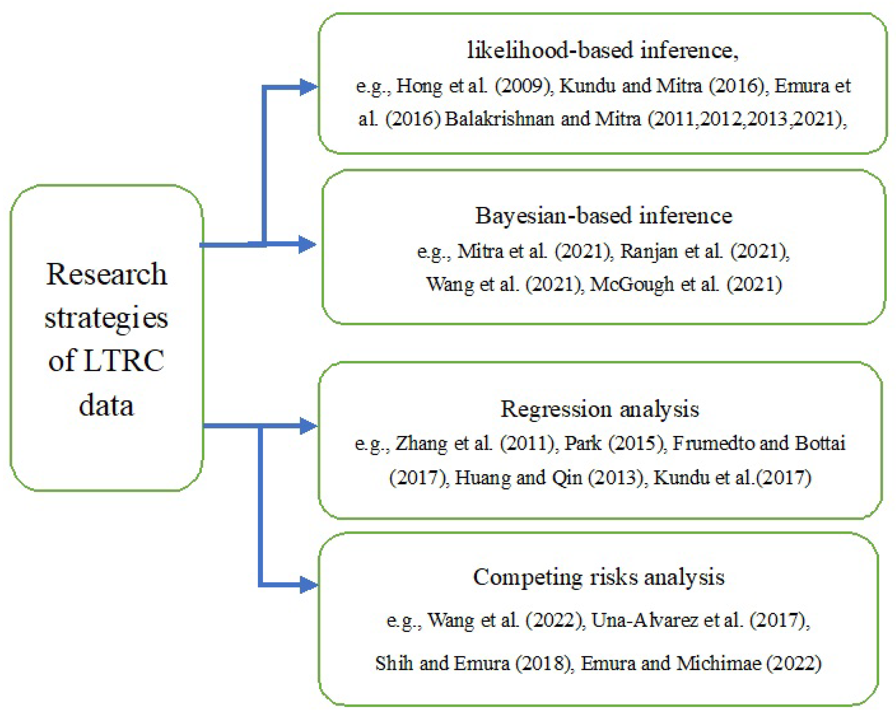
In practical data analysis, failure times usually appear as incomplete data due to experimental limitation such as cost and time constraints. Among various features of incomplete data, truncation and censoring are two most important characteristics frequently appearing in practice. Especially, when units enter the study at a known time point after the time origin, one could obtain data suffering left truncation, whereas for right censoring, it means that the failure times are only known to exceed the prefixed censoring point. Therefore, it is seen that truncation and censoring are classical topics in survival and medical analysis and also widely recognized in both biostatistics and reliability engineering, among other various fields, and that due to complex life-cycle environment and testing conditions, left-truncated and right-censored (LTRC) data as a more widespread phenomenon for failure times are more general in practical situations. For a famous example in engineering, Hong et al. [19] reported an example of LTRC data for voltage power transformers. In this example, there are approximately 150,000 high-voltage power transmission transformers in service in the US. Transformers were installed before or after the year 1980, and the data collection period of failure was conducted by corresponding energy companies between 1980 and 2008. In this case, only complete information for the transformers installed after 1980 and for the transformers installed before 1980 but failed after 1980 is still available, and the transformer information still surviving till 2008 is right-censored in consequence. Thus, the observed transformers failure times appear as LTRC data. Similar real life examples also widely appear in various fields of medical treatment, survival analysis, iostatistics, among others. Therefore, it is meaningful to discuss LTRC data that provides potential theoretical investigation and practical applications in real life analysis and decision-making situations. In literature, inference of LTRC data has been extensively discussed by many authors from various perspectives. To name a few, Hong et al. [19], Balakrishnan and Mitra [20,21,22], Mitra and Balakrishnan [23], Kundu and Mitra [24] with the aid of EM algorithms. Emura et al. [25] compared between the Newton–Raphson (NR) and EM algorithms. The Bayesian analysis of LTRC data from lognormal, Weibull, and gamma distributions was also developed by Mitra et al. [26], Ranjan et al. [27], Wang et al. [28]. Analysis of LTRC data via regression approach along with semiparametric and covariate factors was also discussed by McGough [29], Zhang et al. [30], Park [31], Frumento and Bottai [32], Huang and Qin [33], among others. In addition, when there are multiple failure causes involved, associated LTRC competing risks data were studied by Wang et al. [13], Kundu et al. [34], Wang et al. [35], Una-Alvarez and Veraverbeke [36], Shih and Emura [37], among others. Interested readers may refer to Emura and Michimae [38] for a review. For clarity, Figure 1 is presented to show associated analysis strategies about LTRC data.
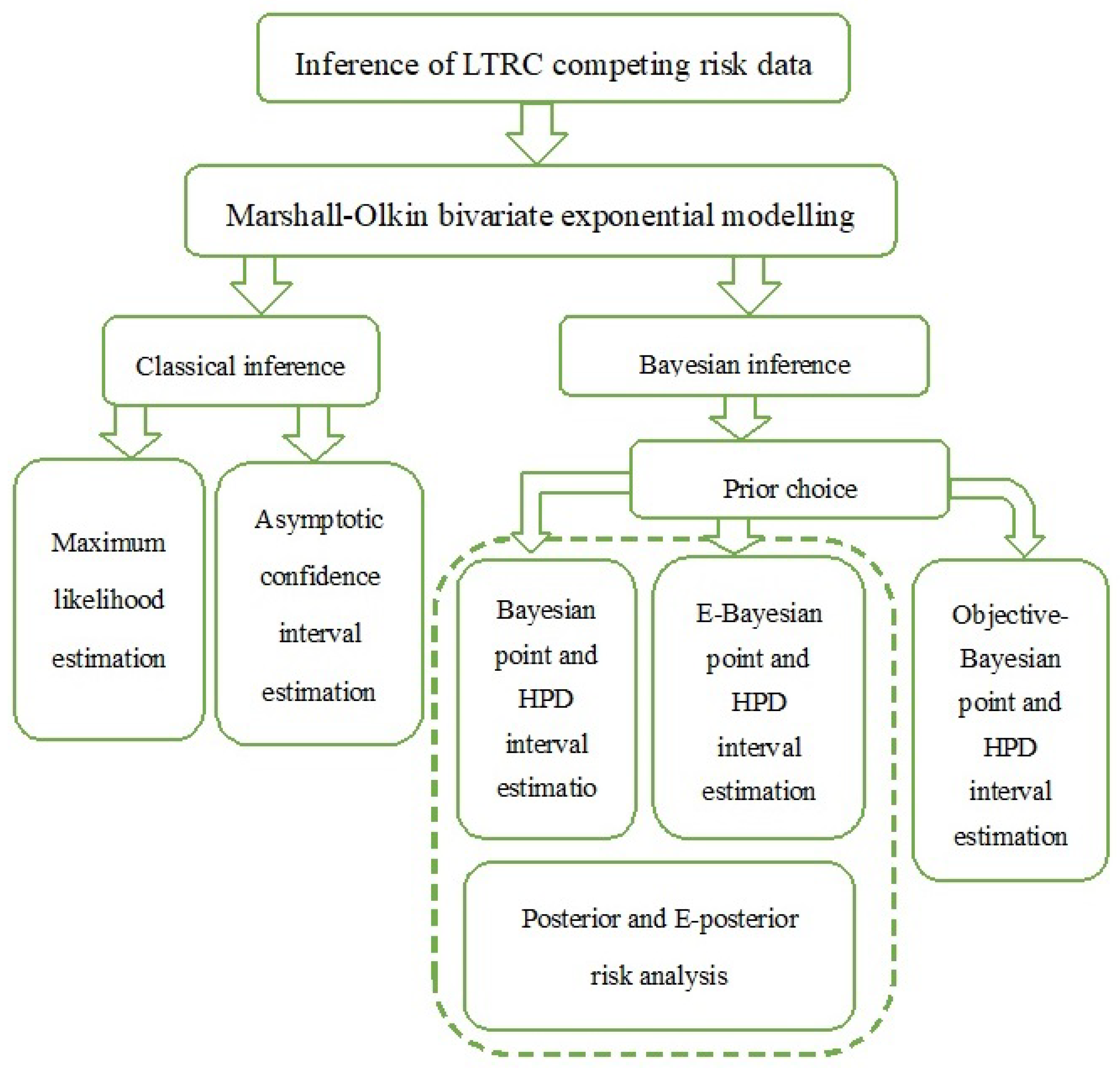
Due to the potential theoretical and practical importance of LTRC data, this paper considers inference for dependent LTRC competing risks data. When the failure causes of LTRC failure time follows a simple shock model, namely the Marshall–Olkin bivariate exponential (MOBE) distribution proposed by Marshall and Olkin [11], estimation for the unknown parameters and the reliability indices are developed under classical and various Bayesian procedures, respectively. The potential novelties and contributions of this paper are as follows. On the one hand, due to the existing literature focusing on independent LTRC competing risks data, this paper considers dependent competing risks data under the LTRC scheme. Although the lifetime of failure causes are modeled by a simpler MOBE distribution, similar results could be obtained when other relatively complex baseline models are used in a Marshall–Olkin-type distributional structure. On the other hand, various Bayesian inferential approaches including traditional, E-Bayesian, and objective-Bayesian estimations are proposed in this paper, and associated risk criterion quantities and asymptotic properties are obtained in different cases. Specifically, it is worth mentioning that in one of our authors’ previous paper [35], inference of dependent LTRC competing risks data is still established, and the common point and difference between these two papers are presented as follows. Firstly, the common point is that the dependent LTRC competing risks data are all modeled by Marshall–Olkin-type distributions in both papers. In paper [35], the lifetime of the causes of risks are discussed based on a Marshall–Olkin-type distribution with Weibull baseline, whereas the exponential-based Marshall–Olkin bivariate distribution is considered in the current paper. Secondly, one main difference is that prior distributions are different between these two papers; a general dependent prior is implemented for model parameters in [35] and the associated results are obtained via Monte Carlo sampling, whereas in the current paper, the independent gamma priors are adopted for incorporating extra prior information under a Bayesian perspective and exact estimators are established subsequently. Finally, comparing with the traditional standard Bayesian estimation in [35], another main difference between two papers is that E-Bayesian and objective Bayesian methods are further proposed in the current paper, where associated estimated risks and E-posterior risks are established and the corresponding asymptotic equivalence is also investigated, and that relatively robust estimates are provided under such scenarios. For illustration, a flowchart about the main contents of the paper is presented in Figure 2. To the best of our knowledge, this problem has not been discussed before in the literature.
The article is organized as follows. In Section 2, the MOBE model and the LTRC data description are introduced. Section 3 establishes the maximum likelihood estimators (MLEs) and the associated approximate confidence intervals (ACIs) for parameters of interest. Conventional Bayesian, E-Bayesian, and objective Bayesian estimations are proposed in Section 4. Simulation studies and two real-life examples are conducted in Section 5. Finally, some brief concluding remarks are presented in Section 6.
2. Model and Data Description
2.1. Marshall–Olkin Bivariate Exponential Distribution
A random variable U follows an exponential distribution with hazard rate when the probability density function (PDF), cumulative distribution function (CDF), and the survival function (SF) of U are respectively given by
This is denoted by .
Let , and be independent exponential random variables satisfying . Define and , then the random vector has the MOBE distribution with parameters , denoted by .
For the sake of simplicity, denote and . Some results of the MOBE model are provided below and the associated proofs are omitted for saving space.
Theorem 1.
Suppose the random vector follows the MOBE distribution with parameters , the joint SF of is given by
Corollary 1.
Suppose the random vector follows the MOBE distribution with parameters , the joint PDF of can be expressed as
Corollary 2.
Suppose the random vector follows the MOBE distribution with parameters , then variable with SF and hazard rate function (HRF) at mission time are given as
It is noted from Theorem 1 that, when , variables and are independent. Therefore, parameter can be regarded as the dependent structure between and . Moreover, it is also noted from Corollary 1 that the probability contributions for events , and are , and , respectively. In addition, it is also seen from Corollary 2 that for units with dependent failure causes following the MOBE model, the associated failure time of the units can be described by the variable .
2.2. Data Description and Notation
Without loss of generality, consider a lifetime experiment with identical units, and their lifetimes are described by independent and identically distributed (i.i.d.) random variables . Corresponding to i-th unit , it is assumed that there is a prefixed left truncation point, say ; each unit can be placed on the test before or after the corresponding left truncation point , and the failure time could be observed only if , otherwise no information is available for the units. In addition, for i-th unit if it survives after , it may be censored after another determining point . In this manner, the obtained observations are referred as LTRC data. Further, for the sake of clarity, the notations used in this paper for the dependent LTRC competing risk data are presented as follows.
- failure time of i-th unit under cause ;
- left-truncated time for the i-th unit;
- right-censored time for the i-th unit;
- observed lifetime of the i-th unit, i.e., ;
- indicator variable for the i-th unit with
- truncated indicator variable for the i-th unit with
- set of indices of censored observations;
- set of indices of failures due to cause and 3;
- cardinality of . It is assumed that .
In this paper, we suppose that there are n LTRC observations with two causes of failure in experiment, and the associated variables of competing risks are satisfying . Therefore, observed data follow . In such manner, the following dependent LTRC competing risks data are obtained as
Theorem 2.
Proof.
See Appendix A. □
From Theorem 2, the likelihood function of parameters , and is
with .
3. Method of Classical Estimation
In this section, MLEs and ACIs are conducted for unknown parameters and reliability indices, respectively.
3.1. Maximum Likelihood Estimation
From (6), the log-likelihood function can be written as
In the following theorem, the MLEs of parameters are established.
Theorem 3.
Proof.
See Appendix B. □
In addition, based on Theorem 3 and using the invariance principle of maximum likelihood estimation, the MLEs of the SF and HRF can be constructed as
with .
3.2. Approximate Confidence Intervals
The Fisher information matrix of parameter vector with is given by
where the elements for are provided as
Under mild regularity conditions, the asymptotic distribution of the MLE is , where is the inverse of the expected Fisher information matrix given by
For arbitrary , a ACI of is given by
where is the upper -th quantile of the standard normal distribution.
Further, let be an arbitrary function of parameter ; then, the asymptotic distribution of can be constructed as
by using the delta method, where the following notations are used: is the MLE of and and . Therefore, the confidence interval of can be constructed subsequently. In this manner, ACIs of the SF and the HRF can be obtained directly and detailed expressions are omitted here for saving space.
4. Method of Bayesian Estimation
In this section, traditional Bayesian, E-Bayesian, and objective Bayesian methods are proposed for parameter and reliability indices estimation, respectively.
4.1. Prior Information and Posterior Analysis
For Bayesian estimation, it is noted that prior information should be incorporated into the inferential procedure. In this section, we adopted the independent gamma distributions to describe the prior information about the model parameters. In statistical inference, the gamma distribution is a flexible distribution that can be used to model different prior information based on proper choice of hyperparameters, it also becomes inversely proportional to its argument when hyperparameters are set to zeros, and some other models such as the Erlang, exponential, and chi-square distributions are special cases of the gamma distribution. In addition, the gamma distribution is also the maximum entropy probability distribution, which also makes this feature an appealing fitting property in different fields such as business, science, and engineering. Therefore, it is assumed that parameters , and are statistically independent, and the gamma conjugate prior for is assumed with hyperparameters and as
Therefore, the joint prior of is given by
and the joint posterior density of can be obtained from (6) and (14) as
implying that the marginal posterior function of the parameter is
which is also the gamma distribution.
Under squared error loss, since the Bayesian estimator is a posterior expectation, the following results are directly obtained and details are omitted for concision.
Theorem 4.
Under squared error loss, one has:
- The Bayesian estimator of the parameter is given by
- The Bayesian estimators of the SF and HRF can be expressed as
It is noted that, sometimes, there are rare prior information collected from historical information or past data; then, flat or non-informative priors may be more proper in this situation. Although gamma priors are adopted in our illustration, the Bayesian results could be also established as a special case under rare or non-information situations by setting all hyperparameters as zero that consequently reduce to non-informative priors. In addition, for an arbitrary significance level , Bayesian highest posterior density (HPD) credible intervals for parameters could be also constructed, and a simple approach namely Algorithm 1 is provided as follows.
| Algorithm 1: Bayesian HPD credible interval estimation |
|
4.2. E-Bayesian Estimation
The expected-Bayesian (E-Bayesian) estimation was firstly proposed by Han [39], and has attracted wide attention and been discussed by many authors. See, for example, some recent works of Basheer et al. [40], Okasha and Wang [41], among others.
Following the idea of Han [39], hyperparameters and should be selected to guarantee that the prior density function decreases in , which implies that and . Under such requirements, the following three independent priors for hyperparameters and are chosen as
Note that since there are no closed forms of the E-Bayesian estimators for reliability indices and , the results are just reported for parameters , and for concision.
Theorem 5.
Under squared error loss and priors , and , the E-Bayesian estimator of can be written respectively as
and
Proof.
See Appendix C. □
Further, using (16) and (19), the posterior densities of parameter with respect to , and can be expressed respectively as
It is seen from (23)–(25) that there are no closed forms of posterior densities for , and under , and . In order to construct E-Bayesian HPD credible intervals, a constrained optimization problem is proposed as follows.
For arbitrary , let
be the Bayesian interval for under prior satisfying that
Thus, the shortest-length credible interval for can be obtained by solving following optimization problem as
This can be further obtained by minimizing the Lagrangian function as
where is the Lagrangian multiplier. Therefore, by using the Lagrangian multiplier method, the Bayesian HPD credible interval for with respect to can be obtained numerically, where and are the solutions of the following nonlinear equations:
4.3. Some Results of Bayesian and E-Bayesian Estimation
In following, the posterior risk (PR) of Bayesian estimators are presented under squared error loss, which generally are used to measure the associated estimated risk of Bayesian estimators.
Theorem 6.
The PR of Bayesian estimators under squared error are obtained as
Proof.
See Appendix D. □
Similarly, another criterion quantity called the E-posterior risk (EPR) is proposed by Han [42] which is an effective measurement for the E-Bayesian estimators.
Theorem 7.
Under square error loss, the EPR of with respect to priors can be expressed respectively as
Proof.
See Appendix E. □
Some relations among various E-Bayesian estimators are also presented as follows.
Theorem 8.
Let , for the E-Bayesian estimators with respect to squared error loss, it is seen that
- ;
- .
Proof.
See Appendix F. □
We note that with respect to priors , and , although E-Bayesian estimators in Theorem 5 are different order relations, they are asymptotically equivalent to each other under the given conditions.
4.4. Objective Bayesian Estimation
Sometimes, prior information is difficult to collect especially when there are rare historical data or a practitioner is not familiar with targeted problems. Therefore, to give a fair inference under the Bayesian approach, objective-Bayesian (O-B) is proposed for eliminating the personal subject effect in priors. Here, objective-Bayesian estimation is proposed in this subsection.
Following Guan et al. [43], a probability matching prior for is given by
Proof.
See Appendix G. □
Therefore, under squared error loss, the O-B estimator of can be expressed as
It is noted that the Bayesian credible intervals cannot be found directly for model parameters from a posterior distribution (35). Alternatively, an important sampling approach namely Algrithm 2 is presented for constructing the Bayesian HPD credible intervals as follows.
| Algorithm 2: Objective Bayesian HPD credible interval estimation |
|
5. Numerical Results and Method Performance
5.1. Simulation Studies
Simulation experiments are conducted for investigating the performance of the proposed methods when dependent LTRC competing risks data are available. The associated point estimates for parameters , and are evaluated in terms of absolute bias (AB) and mean squared error (MSE), and the interval estimates are investigated by the average length (AL) and coverage probability (CP), respectively.
In these simulation studies, values of the hyperparameters are randomly chosen as and , left-truncated proportion , sample sizes , respectively. The simulation procedure is repeated times for the above-designed scenarios, criteria quantities ABs, MSEs, CPs, and ALs are calculated and tabulated in Table 1, Table 2, Table 3 and Table 4, where the significance level is . In addition, for the sake of concision, the numerical results for parameter and the reliability indices are not reported for saving space.
- Under each prior , and , quantities ABs and MSEs of different point estimates (i.e., MLEs and Bayesian results) decrease with an increase of sample size n. A similar phenomenon also appears for both likelihood and Bayes estimates with the decrease of truncation factor p. This indicates that the MLEs and different Bayes estimates feature consistency properties and are satisfactory under design scenarios.
- Under given n and p, the performance of all Bayesian results (i.e., Bayesian, E-Bayesian, and O-Bayesian estimates) are superior to the associated MLEs in terms of ABs and MSEs, in general, under each prior , showing the performance of different results in ascending ranking order as .
- For Bayesian results, the ABs and MSEs of the results from Bayesian and E-Bayesian approaches are relatively smaller than the ones obtained from the O-Bayesian procedure showing the performance of various estimates in ascending ranking order as .
- Under each prior , the ALs of both ACI and HPD credible intervals from different Bayesian approaches decrease when the sample size n increases or the truncation proportion p decreases, and CPs increase under the same trend;
- The CPs of both ACIs and various Bayesian HPD credible intervals are close to the nominal level;
- Under the same settings n and p, the ALs of different Bayesian credible intervals are smaller than those of ACIs in most cases;
- Among all Bayesian intervals, the E-Bayesian credible intervals have the smallest interval lengths whereas the interval estimates from the O-Bayesian approach have the relatively largest interval lengths in general.
To sum up, it is seen from the simulation results that the performance of both likelihood and various Bayesian point and credible interval estimates are preferable, and that the Bayesian and E-Bayesian methods could be viewed as superior choices in our discussion; otherwise, one can use the results obtained from the objective Bayesian approach.
5.2. Real Data Illustrations
Example 1
(Electric Power Transformers Data). In this illustration, the previous mentioned LTRC voltage power transformer LTRC data from the US are discussed. Kundu et al. [34] provided the LTRC competing risks data with exact failure causes, where or 0 indicating that the transformer was installed after or before 1980 but did not fail till 1980, or 2 gives the failure causes one or two of the transformer, respectively, and implies that transformers survived till 2008. In our illustration, since we focus on a more general case with partially observed failure causes, based on Kundu et al. [34]’s LTRC competing risks data, some transformer observations are randomly chosen and denote their associated failure indicator as . Thus, a group of LTRC competing risks data with partially observed failure causes is generated and the details are provided in Table 5. It is clearly seen that comparing with Kundu et al. [34]’s discussion, a more general study is considered with dependent competing risks data and partially recorded failure causes in our illustration.
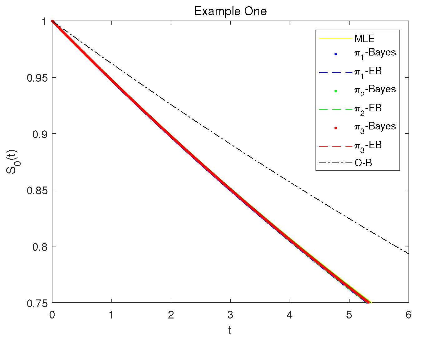
In this example, since there is no extra information for model parameters, Bayesian estimates are obtained with hyperparameters due to the moment matching principle. Under this assumption, second-stage priors , and are proper but almost noninformative with relatively flat curves. Therefore, using the LTRC competing risks data tabulated in Table 5, classical and various Bayesian estimates are obtained in Table 6 with significance level and interval lengths given in squared brackets. It is seen that estimates of MLEs and different Bayes estimates are close to each other, and that the different Bayes HPD credible intervals feature relatively shorter interval lengths than the associated ACIs. In addition, plots of reliability index SF of given in Corollary 2 are presented in Figure 3 based on likelihood and various Bayesian results, where in the associated figure legend, notations “MLE”, “-Bayes” and “-EB” with and “OB” denote that the SFs are plotted by using the point estimates of MLE, Bayes, and E-Bayes estimates with priors , and O-B estimates respectively given in Table 6. It is also observed that SF generally performs similar with respect to different estimates in this illustration.
Example 2
(HIV Infection Data). The AIDSSI dataset about human immunodeficiency virus (HIV) infection in the Amsterdam Cohort Studies is analyzed. In this dataset, 329 homosexual men’s follow-up times (in years) are observed from HIV infection to the first of acquired immunodeficiency syndrome (AIDS) and syncytium-inducing (SI) HIV phenotype. Following Geskus [44], AIDS and SI HIV phenotype are treated as competing failure causes indicated by and 2. For generating LTRC competing risks data, of the observations are randomly chosen from the original data as left-truncated observations, and some failure causes are also randomly taken as unknown with . Thus, a set of LTRC competing risks with partially observed failure causes is generated and presented in Table 7.
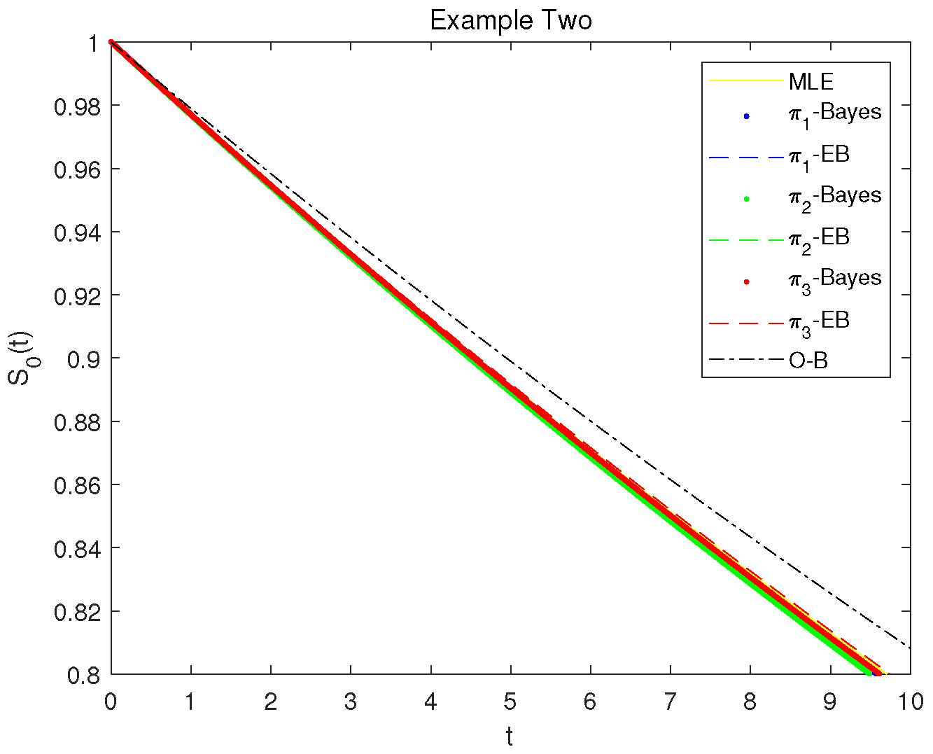
Based on Table 7, following a similar line as Example One, likelihood and Bayesian estimates are presented in Table 8 with and significance level . It is also noted that the performance of both MLEs and Bayes estimates appears similarly, and that the Bayes HPD credible intervals of parameters , and from different priors are superior to the ACIs in terms of interval length, which is consistent with the results of the previous example and simulation studies. Similarly, plots of SF of are also provided in Figure 4 for this case where the notations in the legend of the plot are defined similarly as explained in Example One, and similarity appears as well under the survival medicine competing risks data.
6. Concluding Remarks
In this paper, estimation for dependent competing risks model is discussed under the LTRC scheme. When the lifetime of the causes of failure follows the MOBE distribution, point and interval estimates of unknown parameters as well as reliability indices are obtained in classical and Bayesian procedures, respectively. Besides classical MLEs and ACIs, three types of Bayesian point and interval estimates are also proposed including common Bayesian, E-Bayesian, and objective-Bayesian, respectively. Extensive simulation studies and two real-life examples are carried out for investigating the performance of our methods, and the numerical results show that all classical and Bayesian results perform satisfactory, and that the proposed Bayesian methods are superior to classical likelihood-based results in general. Although inference for LTRC competing risks data is discussed from the MOBE distributions, the scope of this paper can be extended to many other engineering and reliability application fields when other Marshal–Olkin-type bivariate models are available. In addition, there are also limitations in our study. For example, the proposed methods may effectively process relatively simple problems when two random variables are correlated under a shock phenomenon, but cannot completely describe the correlation among complex and multidimensional variable situations. In such cases, one potential approach may refer to the copula function-based method, which seems to be of interest and will be discussed in the future.
Author Contributions
All authors equally contributed in writing this manuscript. All authors have read and agreed to the published version of the manuscript.
Funding
This work was supported by the Yunnan Fundamental Research Projects (No. 202101AT070103) and the Doctoral Research Foundation of Yunnan Normal University (No. 00800205020503129).
Data Availability Statement
Not applicable.
Acknowledgments
Authors would like to thank the Editor and reviewers for their valuable comments and suggestions which improved this paper significantly.
Conflicts of Interest
The authors declare no conflict of interest.
Appendix A. Proof of Theorem 2
For the sake of concision and saving space, although there are eight scenarios for pairs of , we show the results when , and , whereas the remaining results can be obtained in same manner.
For variable , it is conducted that the unit is not truncated and the unit fails at time with failure cause one; then, one equivalently has and . Thus, the associated likelihood contribution refers to
For , the unit is not truncated and the failure occurred at yielded by causes one and two simultaneously, which implies that . Therefore, the associated likelihood contribution can be expressed as
When , it means that the unit is not truncated but right-censored at , which indicates that . So, the associated likelihood contribution can be provided as
Finally, for , it is seen that the unit has been left-truncated indicating that . Moreover, from , one has and . Therefore, the likelihood contribution can be written as
Therefore, the assertion is completed.
Appendix B. Proof of Theorem 3
Taking derivatives of with respect to , respectively, and setting them to zero, estimator could be obtained directly. Further, using inequality for , one has
Therefore, using above inequality, one further has
Since , then it is observed that
where equality holds iff . Therefore, the assertion is completed.
Appendix C. Proof of Theorem 5
Based on prior , the E-Bayesian estimator of is given by
Further, E-Bayesian estimation with priors and can be obtained similarly, and the details are omitted for concision. Therefore, the results are shown.
Appendix D. Proof of Theorem 6
Since the PR can be obtained as the expected loss to the associated posterior density (16) of the targeted parameter, under squared error loss, it is seen that
Therefore, the assertion is completed.
Appendix E. Proof of Theorem 7
From Theorem 8 and Han [42], the EPR of with respect to under square error loss is given by
Moreover, and can be obtained similarly using and . Therefore, the assertion is completed.
Appendix F. Proof of Theorem 8
From the expressions of , it is noted that
Let , using the Taylor expansion , one has that
Based on the above expression, it is observed that for , is equivalent to show which clearly holds for a positive integer . Thus, first-order relations among , and are proved. Furthermore, the second result could be obtained by taking limitations directly. Therefore, the assertion is completed.
Appendix G. Proof of Theorem 9
By direct integration, it is noted that
Denote
then the Jacobian matrix of the transformation is given by
with and .
Based on above re-parameterization, and the result from Gradshteyn and Ryzhik [45] (p. 614, formula 4.635(4)) with
where is the beta function defined by ; then, the integration (A1) can be further rewritten as
Therefore, the posterior distribution of under prior (34) is proper and the assertion is completed.
References
- Rafiee, K.; Feng, Q.; Coitc, D.W. Reliability assessment of competing risks with generalized mixed shock models. Reliab. Eng. Syst. Saf. 2017, 159, 1–11. [Google Scholar] [CrossRef] [Green Version]
- Balakrishnan, N.; So, H.Y.; Ling, M.H. Em algorithm for one-shot device testing with competing risks under Weibull distribution. IEEE Trans. Reliab. 2016, 65, 973–991. [Google Scholar] [CrossRef]
- Varghese, A.S.; Vaidyanatha, V.S. Parameter estimation of Lindley step stress model with independent competing risk under Type-I censoring. Commun. Stat.-Theory Methods 2020, 49, 3026–3043. [Google Scholar] [CrossRef]
- Koley, A.; Kundu, D.; Ganguly, A. Analysis of Type-II hybrid censored competing risks data. Statistics 2017, 51, 1304–1325. [Google Scholar] [CrossRef]
- Moeschberger, M.L. Life tests under dependent competing causes of failure. Technometrics 1974, 16, 39–47. [Google Scholar] [CrossRef]
- Shih, J.H.; Lee, W.; Sun, L.H.; Emura, T. Fitting competing risks data to bivariate Pareto models. Commun.-Stat.-Theory Methods 2019, 48, 1193–1220. [Google Scholar] [CrossRef]
- Fan, T.H.; Wang, Y.F.; Ju, S.K. A competing risks model with multiply censored reliability data under multivariate Weibull distributions. IEEE Trans. Reliab. 2019, 68, 462–475. [Google Scholar] [CrossRef]
- Lorvand, H.; Nematollahi, A.; Poursaeed, M.H. Life distribution properties of a new δ-shock model. Commun.-Stat.-Theory Methods 2020, 49, 3010–3025. [Google Scholar] [CrossRef]
- Gong, M.; Xie, M.; Yang, Y. Reliability assessment of system under a generalized run shock model. J. Appl. Probab. 2018, 55, 1249–1260. [Google Scholar] [CrossRef] [Green Version]
- Lorvand, H.; Kelkinnama, M. Reliability analysis and optimal replacement for a k-out-of-n system under a δ-shock model. J. Risk Reliability 2022. [Google Scholar] [CrossRef]
- Marshall, A.W.; Olkin, I. A multivariate exponential distribution. J. Am. Stat. Assoc. 1967, 62, 30–44. [Google Scholar] [CrossRef]
- Ouyang, T.; He, Y.; Li, H.; Sun, Z.; Baek, S. Modeling and Forecasting Short-Term Power Load With Copula Model and Deep Belief Network. IEEE Trans. Emerg. Top. Comput. Intell. 2019, 3, 127–136. [Google Scholar] [CrossRef] [Green Version]
- Wang, Y.; Emura, T.; Fan, T.; Lo, S.; Wilke, R.A. Likelihood-based inference for a frailty-copula model based on competing risks failure time data. Qual. Reliab. Eng. Int. 2020, 36, 1622–1638. [Google Scholar] [CrossRef]
- Krupskii, P.; Joe, H. Flexible copula models with dynamic dependence and application to financial data. Econom. Stat. 2020, 16, 148–167. [Google Scholar] [CrossRef]
- Bai, X.; Shi, Y.; Liu, Y.; Liu, B. Reliability estimation of multicomponent stress-strength model based on copula function under progressively hybrid censoring. J. Comput. Appl. Math. 2018, 344, 100–144. [Google Scholar] [CrossRef]
- Durante, F. Construction of non-exchangeable bivariate distribution functions. Stat. Pap. 2009, 50, 383–391. [Google Scholar] [CrossRef]
- Amini, A.; Abdollahi, A.; Hariri-Ardebili, M.A.; Lall, U. Copula-based reliability and sensitivity analysis of aging dams: Adaptive Kriging and polynomial chaos Kriging methods. Appl. Soft Comput. 2021, 109, 107524. [Google Scholar] [CrossRef]
- Zhang, C.; Wang, L.; Bai, X.; Huang, J. Bayesian reliability analysis for copula based step-stress partially accelerated dependent competing risks model. Reliab. Eng. Syst. Saf. 2022, 227, 108718. [Google Scholar] [CrossRef]
- Hong, Y.; Meeker, W.Q.; McCalley, J.D. Prediction of remaining life of power transformers based on left truncated and right censored lifetime data. Ann. Appl. Stat. 2009, 857–879. [Google Scholar]
- Balakrishnan, N.; Mitra, D. Likelihood inference for lognormal data with left truncation and right censoring with an illustration. J. Stat. Plan. Inference 2011, 141, 3536–3553. [Google Scholar] [CrossRef]
- Balakrishnan, N.; Mitra, D. Left truncated and right censored weibull data and likelihood inference with an illustration. Comput. Stat. Data Anal. 2012, 56, 4011–4025. [Google Scholar] [CrossRef]
- Balakrishnan, N.; Mitra, D. Likelihood inference based on left truncated and right censored data from a gamma distribution. IEEE Trans. Reliab. 2013, 62, 679–688. [Google Scholar] [CrossRef]
- Mitra, D.; Balakrishnan, D. Statistical inference based on left-truncated and interval censored data from log-location-scale family of distributions. Commun.-Stat.-Theory Methods 2021, 50, 1073–1093. [Google Scholar] [CrossRef]
- Kundu, D.; Mitra, D. Bayesian inference of weibull distribution based on left truncated and right censored data. Comput. Stat. Data Anal. 2016, 99, 38–50. [Google Scholar] [CrossRef]
- Emura, T.; Shiu, S.-K.; Matsui, S. Estimation and model selection for left-truncated and right-censored lifetime data with application to electricpower transformers analysis. Commun.-Stat.-Simul. Comput. 2016, 45, 3171–3189. [Google Scholar] [CrossRef]
- Mitra, D.; Kundu, D.; Balakrishnan, N. Likelihood analysis and stochastic EM algorithm for left truncated right censored data and associated model selection from the Lehmann family of life distributions. J. Stat. Data Sci. 2021, 4, 1019–1048. [Google Scholar] [CrossRef]
- Ranjan, R.; Sen, R.; Upadhyay, S.K. Bayes analysis of some important lifetime models using MCMC based approaches when the observations are left truncated and right censored. Reliab. Eng. Syst. Saf. 2021, 214, 107747. [Google Scholar] [CrossRef]
- Wang, C.; Jiang, J.; Luo, L.; Wang, S. Bayesian analysis of the Box-Cox transformation model based on left-truncated and right-censored data. J. Appl. Stat. 2021, 48, 1429–1441. [Google Scholar] [CrossRef]
- McGough, S.F.; Incerti, D.; Lyalina, S.; Copping, R.; Narasimhan, B.; Tibshirani, R. Penalized regression for left-truncated and right-censored survival data. Stat. Med. 2021, 40, 5487–5500. [Google Scholar] [CrossRef]
- Zhang, X.; Zhang, M.-J.; Fine, J. A proportional hazards regression model for the subdistribution with right-censored and left-truncated competing risks data. Stat. Med. 2011, 30, 1933–1951. [Google Scholar] [CrossRef] [Green Version]
- Park, J. Quantile Regression with Left-Truncated and Right-Censored Data in a Reproducing Kernel Hilbert Space. Commun. Stat. Theory Methods 2015, 44, 1523–1536. [Google Scholar] [CrossRef]
- Frumento, P.; Bottai, M. Parametric modeling of quantile regression coefficient functions with censored and truncated data. Biometrics 2017, 73, 1179–1188. [Google Scholar] [CrossRef] [PubMed]
- Huang, C.-Y.; Qin, J. Semiparametric estimation for the additive hazards model with left-truncated and right-censored data. Biometrika 2013, 100, 877–888. [Google Scholar] [CrossRef] [PubMed] [Green Version]
- Kundu, D.; Mitra, D.; Ganguly, A. Analysis of left truncated and right censored competing risks data. Comput. Stat. Data Anal. 2017, 108, 12–26. [Google Scholar] [CrossRef]
- Wang, L.; Tripathi, Y.M.; Dey, S.; Zhang, C.; Wu, K. Analysis of dependent left-truncated and right-censored competing risks data with partially observed failure causes. Math. Comput. Simulation 2022, 194, 285–307. [Google Scholar] [CrossRef]
- Una-Alvarez, D.J.; Veraverbeke, N. Copula-graphic estimation with left-truncated and right-censored data. Statistics 2017, 51, 387–403. [Google Scholar] [CrossRef]
- Shih, J.H.; Emura, T. Likelihood-based inference for bivariate latent failure time models with competing risks under the generalized FGM copula. Comput. Stat. 2018, 33, 1293–1323. [Google Scholar] [CrossRef]
- Emura, T.; Michimae, H. Left-truncated and right-censored field failure data: Review of parametric analysis for reliability. Qual. Reliab. Eng. Int. 2022, 38, 3919–3934. [Google Scholar] [CrossRef]
- Han, M. The structure of hierarchical prior distribution and its applications. Chin. Oper. Res. Manag. 1997, 63, 31–40. [Google Scholar]
- Basheer, A.M.; Okasha, H.M.; EI-Baz, A.M.; Tarabia, A.M.K. E-bayesian and hierarchical bayesian estimations for the inverse Weibull distribution. Ann. Data Sci. 2021. [Google Scholar] [CrossRef]
- Okasha, H.M.; Wang, J. E-bayesian estimation for the geometric model based on record statistics. Appl. Math. Model. 2016, 40, 658–670. [Google Scholar] [CrossRef]
- Han, M. E-bayesian estimation and its E-posterior risk of the exponential distribution parameter based on complete and type i censored samples. Commun. Stat.-Theory Methods 2020, 49, 1858–1872. [Google Scholar] [CrossRef]
- Guan, Q.; Tang, Y.; Xu, A. Objective Bayesian analysis for bivariate Marshall Olkin exponential distribution. Comput. Stat. Data Anal. 2013, 64, 299–313. [Google Scholar] [CrossRef]
- Geskus, R. Data Analysis with Competing Risks and Intermediate States; CRC Press: Boca Raton, FL, USA, 2016. [Google Scholar]
- Gradshteyn, I.S.; Ryzhik, I.M. Tables of Integrals, Series, and Products; Academic Press: Cambridge, MA, USA, 2007. [Google Scholar]
Figure 1.
Research strategies of LTRC data [19,20,21,22,23,24,25,26,27,28,29,30,31,32,33,34,35,36,37,38].

Figure 2.
Flowchart of the main contents in this paper.

Figure 3.
Plots of SF with different estimates under transformer data.

Figure 4.
Plots of SF with different estimates under HIV infection data.


Table 1.
ABs and MSEs (within bracket) for MOBE competing risks parameters with and .
| Prior | p | n | MLE | Bayes Estimates | E-Bayes Estimates | O-Bayes Estimates | ||||
|---|---|---|---|---|---|---|---|---|---|---|
| 20 | 0.1357 | 0.2021 | 0.1231 | 0.1868 | 0.1221 | 0.1853 | 0.1262 | 0.2136 | ||
| [0.0271] | [0.0716] | [0.0227] | [0.0607] | [0.0213] | [0.0598] | [0.0250] | [0.0797] | |||
| 35 | 0.1065 | 0.1490 | 0.1010 | 0.1424 | 0.1004 | 0.1417 | 0.0968 | 0.1550 | ||
| [0.0162] | [0.0358] | [0.0156] | [0.0336] | [0.0143] | [0.0323] | [0.0143] | [0.401] | |||
| 50 | 0.0926 | 0.1250 | 0.0893 | 0.1214 | 0.0890 | 0.1205 | 0.0839 | 0.1292 | ||
| [0.0129] | [0.0259] | [0.0120] | [0.0242] | [0.0109] | [0.0231] | [0.0115] | [0.0272] | |||
| 20 | 0.1367 | 0.2051 | 0.1238 | 0.1900 | 0.1213 | 0.1890 | 0.1273 | 0.2161 | ||
| [0.0282] | [0.0726] | [0.0232] | [0.0615] | [0.0214] | [0.0604] | [0.0252] | [0.0807] | |||
| 35 | 0.1068 | 0.1533 | 0.1018 | 0.1465 | 0.1017 | 0.1457 | 0.0996 | 0.1597 | ||
| [0.0174] | [0.0396] | [0.0154] | [0.0360] | [0.0145] | [0.0341] | [0.0152] | [0.0429] | |||
| 50 | 0.0939 | 0.1263 | 0.0918 | 0.1227 | 0.0902 | 0.1212 | 0.0868 | 0.1308 | ||
| [0.0132] | [0.0261] | [0.0122] | [0.0244] | [0.0105] | [0.0234] | [0.0117] | [0.0279] | |||
| 20 | 0.1005 | 0.1545 | 0.0911 | 0.1405 | 0.0902 | 0.1401 | 0.0941 | 0.1602 | ||
| [0.0154] | [0.0404] | [0.0126] | [0.0338] | [0.0117] | [0.0314] | [0.0137] | [0.0428] | |||
| 35 | 0.0797 | 0.1124 | 0.0754 | 0.1062 | 0.0751 | 0.1053 | 0.0745 | 0.1158 | ||
| [0.0098] | [0.0208] | [0.0085] | [0.0190] | [0.0076] | [0.0169] | [0.0082] | [0.0210] | |||
| 50 | 0.0696 | 0.0927 | 0.0670 | 0.0915 | 0.0669 | 0.0914 | 0.0653 | 0.0976 | ||
| [0.0073] | [0.0145] | [0.0064] | [0.0139] | [0.0063] | [0.0125] | [0.0063] | [0.0119] | |||
| 20 | 0.1021 | 0.1573 | 0.0927 | 0.1433 | 0.0918 | 0.1431 | 0.0953 | 0.1640 | ||
| [0.0146] | [0.0419] | [0.0129] | [0.0350] | [0.0119] | [0.0332] | [0.0142] | [0.0436] | |||
| 35 | 0.0807 | 0.1138 | 0.0763 | 0.1075 | 0.0754 | 0.1068 | 0.0756 | 0.1174 | ||
| [0.0095] | [0.0213] | [0.0088] | [0.0193] | [0.0082] | [0.0183] | [0.0087] | [0.0227] | |||
| 50 | 0.0708 | 0.0944 | 0.0681 | 0.0921 | 0.0680 | 0.0917 | 0.0664 | 0.0980 | ||
| [0.0075] | [0.0150] | [0.0069] | [0.0142] | [0.0068] | [0.0134] | [0.0069] | [0.0130] | |||
| 20 | 0.2038 | 0.3130 | 0.1859 | 0.2815 | 0.1843 | 0.2794 | 0.1896 | 0.3198 | ||
| [0.0627] | [0.1612] | [0.0516] | [0.1373] | [0.0507] | [0.1350] | [0.0559] | [0.1693] | |||
| 35 | 0.1601 | 0.2241 | 0.1515 | 0.2150 | 0.1514 | 0.2124 | 0.1498 | 0.2317 | ||
| [0.0384] | [0.0846] | [0.0344] | [0.0774] | [0.0323] | [0.0769] | [0.0338] | [0.0816] | |||
| 50 | 0.1386 | 0.1840 | 0.1331 | 0.1783 | 0.1325 | 0.1766 | 0.1298 | 0.1905 | ||
| [0.0287] | [0.0559] | [0.0265] | [0.0527] | [0.0246] | [0.0523] | [0.0254] | [0.0558] | |||
| 20 | 0.2053 | 0.3034 | 0.1862 | 0.2910 | 0.1850 | 0.2888 | 0.1916 | 0.3304 | ||
| [0.0638] | [0.1720] | [0.0525] | [0.1463] | [0.0512] | [0.1439] | [0.0573] | [0.1711] | |||
| 35 | 0.1622 | 0.2255 | 0.1547 | 0.2161 | 0.1532 | 0.2155 | 0.1509 | 0.2325 | ||
| [0.0395] | [0.0852] | [0.0354] | [0.0778] | [0.0338] | [0.0771] | [0.0347] | [0.0822] | |||
| 50 | 0.1401 | 0.1885 | 0.1346 | 0.1837 | 0.1332 | 0.1820 | 0.1312 | 0.1951 | ||
| [0.0296] | [0.0593] | [0.0276] | [0.0557] | [0.0274] | [0.0539] | [0.0265] | [0.0604] | |||
Table 2.
CPs and ALs (within bracket) for MOBE competing risks parameters with and .
| Prior | p | n | MLE | Bayes Estimates | E-Bayes Estimates | O-Bayes Estimates | ||||
|---|---|---|---|---|---|---|---|---|---|---|
| 20 | 0.8650 | 0.9243 | 0.9358 | 0.9244 | 0.9341 | 0.9045 | 0.9418 | 0.9780 | ||
| [0.8217] | [1.0285] | [0.7343] | [1.0108] | [0.7336] | [1.0226] | [0.8083] | [1.0149] | |||
| 35 | 0.9223 | 0.9555 | 0.9486 | 0.9555 | 0.9401 | 0.9529 | 0.9593 | 0.9824 | ||
| [0.6259] | [0.8281] | [0.5865] | [0.8125] | [0.5862] | [0.8024] | [0.6189] | [0.8096] | |||
| 50 | 0.9487 | 0.9837 | 0.9501 | 0.9851 | 0.9588 | 0.9940 | 0.9614 | 0.9895 | ||
| [0.5221] | [0.7817] | [0.5006] | [0.6790] | [0.4896] | [0.7816] | [0.5145] | [0.6730] | |||
| 20 | 0.8223 | 0.9047 | 0.9328 | 0.9239 | 0.9407 | 0.8940 | 0.9327 | 0.9765 | ||
| [0.8235] | [1.1219] | [0.7352] | [1.0221] | [0.7341] | [1.1144] | [0.8077] | [1.0481] | |||
| 35 | 0.9076 | 0.9421 | 0.9342 | 0.9470 | 0.9484 | 0.9471 | 0.9561 | 0.9800 | ||
| [0.6268] | [0.8441] | [0.5872] | [0.8339] | [0.5868] | [0.8239] | [0.6178] | [0.8160] | |||
| 50 | 0.9323 | 0.9744 | 0.9484 | 0.9838 | 0.9650 | 0.9851 | 0.9605 | 0.9814 | ||
| [0.5242] | [0.8185] | [0.5105] | [0.6806] | [0.5007] | [0.7885] | [0.5187] | [0.6745] | |||
| 20 | 0.9275 | 0.9617 | 0.9394 | 0.9851 | 0.9394 | 0.9851 | 0.9618 | 0.9743 | ||
| [0.6167] | [0.8333] | [0.5535] | [0.7644] | [0.5525] | [0.7642] | [0.6046] | [0.8209] | |||
| 35 | 0.9394 | 0.9774 | 0.9483 | 0.9880 | 0.9484 | 0.9882 | 0.9637 | 0.9788 | ||
| [0.4697] | [0.6331] | [0.4402] | [0.6356] | [0.4401] | [0.6138] | [0.4636] | [0.6094] | |||
| 50 | 0.9425 | 0.9816 | 0.9519 | 0.9933 | 0.9520 | 0.9933 | 0.9645 | 0.9803 | ||
| [0.3923] | [0.5836] | [0.3748] | [0.5785] | [0.3743] | [0.5407] | [0.3880] | [0.5045] | |||
| 20 | 0.9158 | 0.9423 | 0.9381 | 0.9832 | 0.9381 | 0.9832 | 0.9622 | 0.9732 | ||
| [0.6229] | [0.8422] | [0.5578] | [0.7719] | [0.5572] | [0.7712] | [0.6101] | [0.8286] | |||
| 35 | 0.9271 | 0.9726 | 0.9468 | 0.9866 | 0.9464 | 0.9866 | 0.9629 | 0.9779 | ||
| [0.4706] | [0.6357] | [0.4510] | [0.6363] | [0.4413] | [0.6156] | [0.4649] | [0.6100] | |||
| 50 | 0.9379 | 0.9764 | 0.9484 | 0.9928 | 0.9498 | 0.9928 | 0.9630 | 0.9813 | ||
| [0.3942] | [0.5878] | [0.3766] | [0.5881] | [0.3770] | [0.5592] | [0.3901] | [0.5061] | |||
| 20 | 0.9261 | 0.9827 | 0.9400 | 0.9854 | 0.9402 | 0.9848 | 0.9610 | 0.9779 | ||
| [1.2326] | [1.6695] | [1.0988] | [1.5316] | [1.0769] | [1.5231] | [1.2092] | [1.6372] | |||
| 35 | 0.9402 | 0.9813 | 0.9444 | 0.9875 | 0.9519 | 0.9854 | 0.9601 | 0.9803 | ||
| [0.9343] | [1.2286] | [0.8754] | [1.2394] | [0.8726] | [1.1804] | [0.9225] | [1.2163] | |||
| 50 | 0.9415 | 0.9863 | 0.9520 | 0.9939 | 0.9520 | 0.9939 | 0.9668 | 0.9809 | ||
| [0.7849] | [1.1752] | [0.7499] | [1.1769] | [0.7311] | [1.0161] | [0.7767] | [1.0071] | |||
| 20 | 0.9248 | 0.9822 | 0.9390 | 0.9829 | 0.9392 | 0.9935 | 0.9580 | 0.9756 | ||
| [1.2391] | [1.6836] | [1.1029] | [1.5424] | [1.1027] | [1.5384] | [1.2143] | [1.6454] | |||
| 35 | 0.9342 | 0.9832 | 0.9509 | 0.9864 | 0.9445 | 0.9875 | 0.9650 | 0.9769 | ||
| [0.9393] | [1.3131] | [0.8799] | [1.2516] | [0.8658] | [1.2292] | [0.9274] | [1.2192] | |||
| 50 | 0.9369 | 0.9837 | 0.9479 | 0.9913 | 0.9479 | 0.9892 | 0.9613 | 0.9781 | ||
| [0.7882] | [1.1805] | [0.7528] | [1.1412] | [0.7525] | [1.1229] | [0.7799] | [1.0121] | |||
Table 3.
ABs and MSEs (within bracket) for MOBE competing risks parameters with and .
| Prior | p | n | MLE | Bayes Estimates | E-Bayes Estimates | O-Bayes Estimates | ||||
|---|---|---|---|---|---|---|---|---|---|---|
| 20 | 0.1010 | 0.2652 | 0.0868 | 0.2507 | 0.0852 | 0.2503 | 0.1092 | 0.2735 | ||
| [0.0154] | [0.1213] | [0.0113] | [0.1071] | [0.0117] | [0.1063] | [0.0192] | [0.1293] | |||
| 35 | 0.0762 | 0.2104 | 0.0691 | 0.2036 | 0.0685 | 0.2031 | 0.0778 | 0.2157 | ||
| [0.0089] | [0.0747] | [0.0072] | [0.0695] | [0.0069] | [0.0691] | [0.0093] | [0.0784] | |||
| 50 | 0.0632 | 0.1840 | 0.0594 | 0.1797 | 0.0591 | 0.1793 | 0.0632 | 0.1881 | ||
| [0.0060] | [0.0558] | [0.0056] | [0.0533] | [0.0049] | [0.0530] | [0.0056] | [0.0582] | |||
| 20 | 0.1022 | 0.2660 | 0.0878 | 0.2511 | 0.0859 | 0.2458 | 0.1112 | 0.2744 | ||
| [0.0164] | [0.1223] | [0.0125] | [0.1078] | [0.0118] | [0.1070] | [0.0196] | [0.1305] | |||
| 35 | 0.0767 | 0.2117 | 0.0704 | 0.2046 | 0.0698 | 0.2049 | 0.0782 | 0.2173 | ||
| [0.0092] | [0.0759] | [0.0076] | [0.0705] | [0.0083] | [0.0707] | [0.0097] | [0.0797] | |||
| 50 | 0.0638 | 0.1847 | 0.0601 | 0.1806 | 0.0593 | 0.1802 | 0.0639 | 0.1889 | ||
| [0.0063] | [0.0565] | [0.0061] | [0.0538] | [0.0052] | [0.0535] | [0.0064] | [0.0589] | |||
| 20 | 0.0761 | 0.2015 | 0.0653 | 0.1898 | 0.0651 | 0.1896 | 0.0823 | 0.2073 | ||
| [0.0091] | [0.0711] | [0.0065] | [0.0624] | [0.0062] | [0.0621] | [0.0110] | [0.0756] | |||
| 35 | 0.0565 | 0.1561 | 0.0515 | 0.1503 | 0.0512 | 0.1509 | 0.0576 | 0.1502 | ||
| [0.0048] | [0.0403] | [0.0041] | [0.0378] | [0.0040] | [0.0381] | [0.0051] | [0.0430] | |||
| 50 | 0.0472 | 0.1337 | 0.0438 | 0.1306 | 0.0431 | 0.1303 | 0.0471 | 0.1367 | ||
| [0.0035] | [0.0297] | [0.0031] | [0.0282] | [0.0029] | [0.0273] | [0.0032] | [0.0310] | |||
| 20 | 0.0776 | 0.2041 | 0.0662 | 0.1922 | 0.0659 | 0.1919 | 0.0844 | 0.2105 | ||
| [0.0096] | [0.0731] | [0.0069] | [0.0640] | [0.0066] | [0.0639] | [0.0115] | [0.0779] | |||
| 35 | 0.0569 | 0.1563 | 0.0521 | 0.1516 | 0.0518 | 0.1512 | 0.0581 | 0.1601 | ||
| [0.0051] | [0.0410] | [0.0046] | [0.0384] | [0.0043] | [0.0382] | [0.0056] | [0.0433] | |||
| 50 | 0.0474 | 0.1378 | 0.0444 | 0.1347 | 0.0434 | 0.1341 | 0.0475 | 0.1409 | ||
| [0.0038] | [0.0311] | [0.0037] | [0.0296] | [0.0035] | [0.0289] | [0.0036] | [0.0324] | |||
| 20 | 0.1511 | 0.4013 | 0.1305 | 0.3793 | 0.1284 | 0.3775 | 0.1633 | 0.4127 | ||
| [0.0366] | [0.2817] | [0.0264] | [0.2481] | [0.0261] | [0.2466] | [0.0434] | [0.3001] | |||
| 35 | 0.1146 | 0.3112 | 0.1047 | 0.3014 | 0.1043 | 0.3009 | 0.1162 | 0.3190 | ||
| [0.0205] | [0.1626] | [0.0171] | [0.1519] | [0.0167] | [0.1513] | [0.0216] | [0.1708] | |||
| 50 | 0.0847 | 0.2708 | 0.0884 | 0.2648 | 0.0873 | 0.2645 | 0.0944 | 0.2770 | ||
| [0.0130] | [0.1208] | [0.0120] | [0.1152] | [0.0113] | [0.1150] | [0.0140] | [0.1218] | |||
| 20 | 0.1542 | 0.4022 | 0.1333 | 0.3786 | 0.1310 | 0.3802 | 0.1674 | 0.4148 | ||
| [0.0373] | [0.2823] | [0.0276] | [0.2495] | [0.0265] | [0.2470] | [0.0447] | [0.3011] | |||
| 35 | 0.1161 | 0.3220 | 0.1062 | 0.3117 | 0.1057 | 0.3112 | 0.1185 | 0.3301 | ||
| [0.0212] | [0.1735] | [0.0175] | [0.1603] | [0.0170] | [0.1569] | [0.0224] | [0.1820] | |||
| 50 | 0.0949 | 0.2780 | 0.0889 | 0.2718 | 0.0879 | 0.2715 | 0.0950 | 0.2843 | ||
| [0.0141] | [0.1264] | [0.0123] | [0.1203] | [0.0121] | [0.1200] | [0.0143] | [0.1260] | |||
Table 4.
CPs and ALs (within bracket) for MOBE competing risks parameters with and .
| Prior | p | n | MLE | Bayes Estimates | E-Bayes Estimates | O-Bayes Estimates | ||||
|---|---|---|---|---|---|---|---|---|---|---|
| 20 | 0.9423 | 0.9700 | 0.9741 | 0.9814 | 0.9742 | 0.9815 | 0.9906 | 0.9583 | ||
| [0.7732] | [1.4377] | [0.6380] | [1.3264] | [0.6373] | [1.3250] | [0.7445] | [1.3970] | |||
| 35 | 0.9755 | 0.9737 | 0.9797 | 0.9931 | 0.9797 | 0.9931 | 0.9871 | 0.9646 | ||
| [0.5656] | [1.3027] | [0.5109] | [1.1026] | [0.5108] | [1.0597] | [0.5567] | [1.1096] | |||
| 50 | 0.9784 | 0.9779 | 0.9842 | 0.9942 | 0.9834 | 0.9939 | 0.9912 | 0.9753 | ||
| [0.4663] | [1.2108] | [0.4388] | [1.0245] | [0.4367] | [0.9816] | [0.4324] | [1.0775] | |||
| 20 | 0.9414 | 0.9698 | 0.9721 | 0.9799 | 0.9722 | 0.9800 | 0.9857 | 0.9579 | ||
| [0.7769] | [1.4384] | [0.6405] | [1.3308] | [0.6401] | [1.3302] | [0.7477] | [1.4025] | |||
| 35 | 0.9738 | 0.9720 | 0.9771 | 0.9914 | 0.9775 | 0.9914 | 0.9899 | 0.9652 | ||
| [0.5690] | [1.3066] | [0.5142] | [1.2066] | [0.5138] | [1.0752] | [0.5600] | [1.1552] | |||
| 50 | 0.9783 | 0.9757 | 0.9834 | 0.9939 | 0.9843 | 0.9933 | 0.9906 | 0.9747 | ||
| [0.4733] | [1.2121] | [0.4396] | [1.1122] | [0.4394] | [1.0853] | [0.4674] | [0.9781] | |||
| 20 | 0.9447 | 0.9682 | 0.9726 | 0.9788 | 0.9728 | 0.9789 | 0.9877 | 0.9606 | ||
| [0.5854] | [1.0732] | [0.4836] | [0.9923] | [0.4635] | [0.9891] | [0.5567] | [0.0450] | |||
| 35 | 0.9772 | 0.9756 | 0.9787 | 0.9927 | 0.9789 | 0.9928 | 0.9905 | 0.9683 | ||
| [0.4249] | [0.9150] | [0.3814] | [0.8731] | [0.3733] | [0.7931] | [0.4175] | [0.7859] | |||
| 50 | 0.9796 | 0.9800 | 0.9811 | 0.9941 | 0.9813 | 0.9943 | 0.9911 | 0.9720 | ||
| [0.3527] | [0.9010] | [0.3263] | [0.9012] | [0.3159] | [0.6607] | [0.3481] | [0.6554] | |||
| 20 | 0.9421 | 0.9656 | 0.9710 | 0.9780 | 0.9709 | 0.9782 | 0.9862 | 0.9583 | ||
| [0.5791] | [1.0841] | [0.4872] | [1.0011] | [0.4792] | [1.0001] | [0.5619] | [1.0548] | |||
| 35 | 0.9739 | 0.9761 | 0.9774 | 0.9922 | 0.9774 | 0.9922 | 0.9894 | 0.9680 | ||
| [0.4241] | [0.9164] | [0.3838] | [0.9024] | [0.3806] | [0.8054] | [0.4183] | [0.7881] | |||
| 50 | 0.9776 | 0.9796 | 0.9807 | 0.9924 | 0.9808 | 0.9925 | 0.9899 | 0.9704 | ||
| [0.3543] | [0.9323] | [0.3297] | [0.8865] | [0.3179] | [0.6631] | [0.3497] | [0.6578] | |||
| 20 | 0.9424 | 0.9683 | 0.9714 | 0.9793 | 0.9715 | 0.9794 | 0.9887 | 0.9628 | ||
| [1.1588] | [2.1473] | [0.9341] | [1.9255] | [0.9317] | [1.8954] | [1.1144] | [2.0916] | |||
| 35 | 0.9745 | 0.9840 | 0.9787 | 0.9927 | 0.9787 | 0.9928 | 0.9901 | 0.9689 | ||
| [0.8472] | [1.8912] | [0.7636] | [1.6782] | [0.7568] | [1.5485] | [0.8344] | [1.5740] | |||
| 50 | 0.9781 | 0.9776 | 0.9849 | 0.9935 | 0.9850 | 0.9940 | 0.9909 | 0.9733 | ||
| [0.7054] | [1.3230] | [0.6523] | [1.2612] | [0.6504] | [1.1151] | [0.6962] | [1.3117] | |||
| 20 | 0.9412 | 0.9678 | 0.9452 | 0.9783 | 0.9701 | 0.9783 | 0.9851 | 0.9580 | ||
| [1.1630] | [2.1563] | [0.9490] | [1.9464] | [0.9420] | [1.9063] | [1.1207] | [2.1019] | |||
| 35 | 0.9713 | 0.9765 | 0.9700 | 0.9917 | 0.9751 | 0.9916 | 0.9891 | 0.9626 | ||
| [0.8504] | [1.9912] | [0.7658] | [1.7157] | [0.7619] | [1.6429] | [0.8368] | [1.5808] | |||
| 50 | 0.9792 | 0.9752 | 0.9828 | 0.9923 | 0.9829 | 0.9935 | 0.9899 | 0.9729 | ||
| [0.7082] | [1.3286] | [0.6577] | [1.2716] | [0.6538] | [1.2316] | [0.6991] | [1.3122] | |||
Table 5.
LTRC transformers’ competing risks data with partially observed failure causes.
| No. | IY | EY | No. | IY | EY | No. | IY | EY | ||||||
|---|---|---|---|---|---|---|---|---|---|---|---|---|---|---|
| 1 | 1961 | 1996 | 0 | 2 | 11 | 1963 | 2008 | 0 | 3 | 21 | 1960 | 1988 | 0 | 1 |
| 2 | 1964 | 1985 | 0 | 1 | 12 | 1963 | 2000 | 0 | 1 | 22 | 1961 | 1993 | 0 | 2 |
| 3 | 1962 | 2007 | 0 | 2 | 13 | 1960 | 1981 | 0 | 2 | 23 | 1961 | 1990 | 0 | 2 |
| 4 | 1962 | 1986 | 0 | 2 | 14 | 1963 | 1984 | 0 | 2 | 24 | 1960 | 1986 | 0 | 1 |
| 5 | 1961 | 1992 | 0 | 2 | 15 | 1963 | 1993 | 0 | 2 | 25 | 1962 | 2008 | 0 | 3 |
| 6 | 1962 | 1987 | 0 | 1 | 16 | 1964 | 1992 | 0 | 2 | 26 | 1964 | 1982 | 0 | 2 |
| 7 | 1964 | 1993 | 0 | 2 | 17 | 1961 | 1981 | 0 | 2 | 27 | 1963 | 1984 | 0 | 1 |
| 8 | 1960 | 1984 | 0 | 2 | 18 | 1960 | 1995 | 0 | 1 | 28 | 1960 | 1987 | 0 | 2 |
| 9 | 1963 | 1997 | 0 | 2 | 19 | 1961 | 2008 | 0 | 3 | 29 | 1962 | 1996 | 0 | 2 |
| 10 | 1962 | 1995 | 0 | 2 | 20 | 1960 | 2002 | 0 | 1 | 30 | 1963 | 1994 | 0 | 1 |
| 31 | 1987 | 2008 | 1 | 3 | 41 | 1980 | 2008 | 1 | 3 | 51 | 1984 | 2001 | 1 | 2 |
| 32 | 1980 | 2008 | 1 | 3 | 42 | 1982 | 2008 | 1 | 3 | 52 | 1983 | 2008 | 1 | 3 |
| 33 | 1988 | 2008 | 1 | 0 | 43 | 1986 | 2008 | 1 | 0 | 53 | 1988 | 2008 | 1 | 3 |
| 34 | 1985 | 2008 | 1 | 3 | 44 | 1984 | 2008 | 1 | 3 | 54 | 1988 | 2008 | 1 | 0 |
| 35 | 1989 | 2008 | 1 | 3 | 45 | 1986 | 1995 | 1 | 2 | 55 | 1985 | 2008 | 1 | 3 |
| 36 | 1981 | 2008 | 1 | 0 | 46 | 1986 | 2008 | 1 | 3 | 56 | 1986 | 2008 | 1 | 0 |
| 37 | 1985 | 2008 | 1 | 3 | 47 | 1987 | 2008 | 1 | 3 | 57 | 1988 | 2008 | 1 | 3 |
| 38 | 1986 | 2004 | 1 | 2 | 48 | 1986 | 2008 | 1 | 0 | 58 | 1982 | 2008 | 1 | 3 |
| 39 | 1980 | 1987 | 1 | 2 | 49 | 1986 | 2008 | 1 | 0 | 59 | 1985 | 2008 | 1 | 0 |
| 40 | 1986 | 2005 | 1 | 1 | 50 | 1984 | 2008 | 1 | 3 | 60 | 1988 | 2008 | 1 | 3 |
| 61 | 1982 | 2004 | 1 | 2 | 71 | 1989 | 2008 | 1 | 3 | 81 | 1981 | 2006 | 1 | 2 |
| 62 | 1980 | 2008 | 1 | 3 | 72 | 1989 | 2008 | 1 | 3 | 82 | 1988 | 1996 | 1 | 1 |
| 63 | 1980 | 2002 | 1 | 2 | 73 | 1986 | 2008 | 1 | 3 | 83 | 1985 | 2002 | 1 | 2 |
| 64 | 1984 | 2008 | 1 | 3 | 74 | 1982 | 1999 | 1 | 2 | 84 | 1984 | 2008 | 1 | 0 |
| 65 | 1981 | 1999 | 1 | 1 | 75 | 1985 | 2008 | 1 | 3 | 85 | 1980 | 2008 | 1 | 3 |
| 66 | 1986 | 2007 | 1 | 2 | 76 | 1986 | 2008 | 1 | 3 | 86 | 1982 | 2008 | 1 | 0 |
| 67 | 1987 | 2008 | 1 | 0 | 77 | 1982 | 2008 | 1 | 3 | 87 | 1981 | 1995 | 1 | 2 |
| 68 | 1983 | 2008 | 1 | 3 | 78 | 1988 | 2004 | 1 | 1 | 88 | 1986 | 1997 | 1 | 2 |
| 69 | 1983 | 2006 | 1 | 2 | 79 | 1980 | 2008 | 1 | 3 | 89 | 1986 | 2008 | 1 | 3 |
| 70 | 1983 | 1993 | 1 | 1 | 80 | 1982 | 2002 | 1 | 2 | 90 | 1986 | 2008 | 1 | 3 |
| 91 | 1982 | 2008 | 1 | 3 | 96 | 1986 | 2008 | 1 | 0 | |||||
| 92 | 1989 | 2008 | 1 | 0 | 97 | 1982 | 1996 | 1 | 2 | |||||
| 93 | 1984 | 2008 | 1 | 0 | 98 | 1982 | 2008 | 1 | 0 | |||||
| 94 | 1980 | 2008 | 1 | 0 | 99 | 1982 | 2008 | 1 | 0 | |||||
| 95 | 1988 | 2008 | 1 | 0 | 100 | 1989 | 2008 | 1 | 0 |
Note: abbreviation “IY” refers to “Instal year”, “EY” denotes “Exit year”, respectively.
Table 6.
Point and interval estimates of MOBE parameters for dependent electric power transformers’ competing risks data.
Table 6.
Point and interval estimates of MOBE parameters for dependent electric power transformers’ competing risks data.
| Estimates | ||||
|---|---|---|---|---|
| MLE | 0.0081 | 0.0192 | 0.0262 | |
| Bayes | 0.0084 | 0.0194 | 0.0264 | |
| E-B | 0.0083 | 0.0194 | 0.0263 | |
| Bayes | 0.0084 | 0.0193 | 0.0261 | |
| E-B | 0.0085 | 0.0195 | 0.0264 | |
| Bayes | 0.0084 | 0.0194 | 0.0262 | |
| E-B | 0.0084 | 0.0192 | 0.0264 | |
| O-B estimates | 0.0083 | 0.0194 | 0.0110 | |
| ACI | (0.0039,0.0168)[0.0129] | (0.0143,0.0256)[0.0113] | (0.0206,0.0333)[0.0127] | |
| B-HPD | (0.0082,0.0133)[0.0051] | (0.0191,0.0245)[0.0054] | (0.0260,0.0315)[0.0055] | |
| E-B HPD | (0.0081,0.0128)[0.0047] | (0.0190,0.0241)[0.0051] | (0.0261,0.0314)[0.0052] | |
| B-HPD | (0.0083,0.0134)[0.0051] | (0.0192,0.0245)[0.0053] | (0.0259,0.0313)[0.0054] | |
| E-B HPD | (0.0084,0.0133)[0.0049] | (0.0193,0.0243)[0.0050] | (0.0262,0.0319)[0.0057] | |
| B-HPD | (0.0080,0.0129)[0.0049] | (0.0192,0.0245)[0.0053] | (0.0261,0.0317)[0.0056] | |
| E-B HPD | (0.0083,0.0130)[0.0047] | (0.0189,0.0242)[0.0053] | (0.0263,0.0316)[0.0053] | |
| O-B HPD | (0.0081,0.0130)[0.0049] | (0.0191,0.0243)[0.0052] | (0.0110,0.0166)[0.0056] | |
Table 7.
Left-truncated and right-censored HIV infection competing risks data.
| No. | Time | No. | Time | No. | Time | No. | Time | No. | Time | ||||||||||
|---|---|---|---|---|---|---|---|---|---|---|---|---|---|---|---|---|---|---|---|
| 1 | 9.106 | 1 | 1 | 11 | 9.895 | 0 | 1 | 21 | 8.755 | 1 | 1 | 31 | 13.405 | 1 | 3 | 41 | 0.531 | 1 | 3 |
| 2 | 11.039 | 1 | 3 | 12 | 6.218 | 1 | 2 | 22 | 13.44 | 0 | 3 | 32 | 13.424 | 0 | 3 | 42 | 7.636 | 1 | 3 |
| 3 | 2.234 | 0 | 1 | 13 | 6.82 | 1 | 2 | 23 | 8.191 | 1 | 1 | 33 | 5.106 | 1 | 2 | 43 | 7.302 | 1 | 1 |
| 4 | 9.878 | 1 | 2 | 14 | 5.054 | 1 | 3 | 24 | 5.525 | 1 | 2 | 34 | 10.453 | 0 | 1 | 44 | 6.85 | 1 | 2 |
| 5 | 3.819 | 1 | 1 | 15 | 10.196 | 1 | 1 | 25 | 11.529 | 1 | 3 | 35 | 7.409 | 0 | 2 | 45 | 8.586 | 0 | 1 |
| 6 | 6.801 | 0 | 1 | 16 | 1.503 | 0 | 2 | 26 | 2.705 | 1 | 1 | 36 | 6.018 | 1 | 2 | 46 | 3.639 | 1 | 1 |
| 7 | 3.953 | 1 | 1 | 17 | 1.259 | 1 | 0 | 27 | 2.672 | 1 | 1 | 37 | 12.999 | 1 | 3 | 47 | 6.439 | 1 | 2 |
| 8 | 8.605 | 1 | 2 | 18 | 6.549 | 1 | 3 | 28 | 1.889 | 1 | 2 | 38 | 13.495 | 1 | 0 | 48 | 0.884 | 1 | 2 |
| 9 | 10.078 | 1 | 1 | 19 | 13.405 | 1 | 3 | 29 | 3.724 | 1 | 1 | 39 | 9.694 | 1 | 1 | 49 | 4.394 | 1 | 2 |
| 10 | 5.018 | 1 | 1 | 20 | 13.311 | 1 | 3 | 30 | 5.251 | 0 | 1 | 40 | 5.667 | 0 | 1 | 50 | 8.142 | 1 | 2 |
| 51 | 9.363 | 1 | 3 | 61 | 1.456 | 1 | 3 | 71 | 5.618 | 1 | 1 | 81 | 10.563 | 1 | 3 | 91 | 3.562 | 0 | 3 |
| 52 | 11.269 | 1 | 3 | 62 | 12.129 | 1 | 1 | 72 | 10.889 | 1 | 1 | 82 | 8.657 | 1 | 3 | 92 | 8.358 | 0 | 1 |
| 53 | 0.148 | 1 | 0 | 63 | 7.904 | 1 | 2 | 73 | 13.221 | 1 | 3 | 83 | 5.336 | 1 | 2 | 93 | 1.205 | 1 | 2 |
| 54 | 13.402 | 0 | 3 | 64 | 7.17 | 1 | 2 | 74 | 13.32 | 1 | 3 | 84 | 2.177 | 1 | 1 | 94 | 1.101 | 1 | 2 |
| 55 | 4.118 | 0 | 3 | 65 | 13.191 | 1 | 3 | 75 | 9.897 | 1 | 2 | 85 | 4.608 | 1 | 1 | 95 | 5.766 | 1 | 3 |
| 56 | 6.979 | 1 | 2 | 66 | 5.886 | 1 | 2 | 76 | 5.889 | 1 | 2 | 86 | 6.054 | 1 | 1 | 96 | 4.066 | 0 | 3 |
| 57 | 6.955 | 1 | 1 | 67 | 5.082 | 1 | 2 | 77 | 1.593 | 0 | 2 | 87 | 13.323 | 1 | 3 | 97 | 3.195 | 1 | 1 |
| 58 | 2.322 | 1 | 2 | 68 | 8.638 | 0 | 1 | 78 | 3.513 | 1 | 1 | 88 | 6.943 | 1 | 2 | 98 | 0.969 | 1 | 2 |
| 59 | 10.903 | 1 | 1 | 69 | 5.9 | 0 | 3 | 79 | 6.494 | 1 | 3 | 89 | 11.469 | 1 | 1 | 99 | 2.798 | 0 | 2 |
| 60 | 10.067 | 1 | 1 | 70 | 7.184 | 1 | 3 | 80 | 2.866 | 1 | 2 | 90 | 3.647 | 1 | 1 | 100 | 3.94 | 1 | 2 |
| 101 | 0.474 | 0 | 2 | 111 | 11.201 | 1 | 1 | 121 | 6.177 | 0 | 1 | 131 | 9.566 | 1 | 2 | 141 | 7.553 | 1 | 1 |
| 102 | 5.9 | 1 | 3 | 112 | 5.867 | 0 | 3 | 122 | 1.837 | 1 | 1 | 132 | 5.563 | 1 | 2 | 142 | 4.4 | 1 | 2 |
| 103 | 12.934 | 1 | 3 | 113 | 3.88 | 1 | 2 | 123 | 10.303 | 0 | 1 | 133 | 10.53 | 0 | 1 | 143 | 9.793 | 1 | 0 |
| 104 | 3.439 | 1 | 2 | 114 | 3.797 | 1 | 2 | 124 | 5.821 | 1 | 3 | 134 | 6.111 | 1 | 3 | 144 | 2.283 | 1 | 1 |
| 105 | 0.619 | 0 | 3 | 115 | 3.003 | 0 | 3 | 125 | 13.325 | 1 | 3 | 135 | 9.473 | 0 | 1 | 145 | 8.632 | 1 | 3 |
| 106 | 6.224 | 1 | 1 | 116 | 13.363 | 1 | 3 | 126 | 2.368 | 1 | 3 | 136 | 9.555 | 0 | 1 | 146 | 5.454 | 0 | 2 |
| 107 | 7.751 | 1 | 2 | 117 | 10.223 | 1 | 0 | 127 | 12.934 | 0 | 3 | 137 | 12.934 | 1 | 3 | 147 | 9.221 | 1 | 3 |
| 108 | 0.824 | 1 | 2 | 118 | 9.437 | 1 | 2 | 128 | 4.099 | 1 | 1 | 138 | 6.289 | 1 | 3 | 148 | 9.07 | 0 | 1 |
| 109 | 13.432 | 1 | 0 | 119 | 9.137 | 0 | 1 | 129 | 13.131 | 1 | 0 | 139 | 11.02 | 1 | 2 | 149 | 8.783 | 0 | 3 |
| 110 | 10.617 | 1 | 2 | 120 | 2.533 | 1 | 1 | 130 | 3.064 | 1 | 1 | 140 | 2.316 | 0 | 3 | 150 | 6.532 | 1 | 3 |
| 151 | 13.396 | 1 | 3 | 161 | 9.07 | 1 | 2 | 171 | 12.4 | 1 | 2 | 181 | 4.523 | 1 | 2 | 191 | 5.938 | 1 | 1 |
| 152 | 13.12 | 0 | 3 | 162 | 13.287 | 1 | 3 | 172 | 4.854 | 1 | 2 | 182 | 13.432 | 1 | 0 | 192 | 5.12 | 1 | 2 |
| 153 | 9.733 | 1 | 1 | 163 | 5.7 | 1 | 2 | 173 | 8.066 | 1 | 1 | 183 | 5.494 | 1 | 0 | 193 | 4.033 | 1 | 2 |
| 154 | 5.703 | 1 | 2 | 164 | 13.284 | 1 | 3 | 174 | 5.723 | 0 | 1 | 184 | 6.045 | 0 | 1 | 194 | 6.042 | 1 | 1 |
| 155 | 4.389 | 1 | 2 | 165 | 6.733 | 0 | 1 | 175 | 3.373 | 0 | 1 | 185 | 3.584 | 1 | 2 | 195 | 6.511 | 1 | 2 |
| 156 | 1.462 | 1 | 2 | 166 | 13.377 | 0 | 0 | 176 | 11.696 | 0 | 2 | 186 | 13.432 | 0 | 0 | 196 | 0.652 | 1 | 0 |
| 157 | 1.44 | 1 | 1 | 167 | 5.73 | 1 | 2 | 177 | 3.22 | 1 | 2 | 187 | 3.477 | 1 | 1 | 197 | 1.013 | 1 | 2 |
| 158 | 5.555 | 1 | 1 | 168 | 7.781 | 1 | 1 | 178 | 1.166 | 1 | 0 | 188 | 5.908 | 1 | 2 | 198 | 5.736 | 1 | 2 |
| 159 | 0.137 | 1 | 2 | 169 | 10.847 | 1 | 1 | 179 | 8.564 | 1 | 0 | 189 | 4.966 | 1 | 2 | 199 | 6.199 | 1 | 1 |
| 160 | 0.142 | 0 | 3 | 170 | 1.687 | 0 | 3 | 180 | 5.478 | 1 | 2 | 190 | 5.566 | 0 | 1 | 200 | 10.73 | 1 | 1 |
| 201 | 2.982 | 1 | 2 | 211 | 4.219 | 1 | 1 | 221 | 5.021 | 1 | 2 | 231 | 2.513 | 1 | 2 | 241 | 9.44 | 0 | 2 |
| 202 | 2.155 | 1 | 1 | 212 | 11.387 | 1 | 1 | 222 | 5.224 | 1 | 2 | 232 | 12.876 | 1 | 0 | 242 | 13.188 | 1 | 0 |
| 203 | 13.383 | 1 | 0 | 213 | 4.214 | 1 | 0 | 223 | 13.281 | 1 | 0 | 233 | 6.311 | 1 | 2 | 243 | 7.537 | 1 | 2 |
| 204 | 2.683 | 1 | 1 | 214 | 8.986 | 1 | 1 | 224 | 7.349 | 0 | 1 | 234 | 1.509 | 1 | 0 | 244 | 2.571 | 0 | 2 |
| 205 | 4.811 | 1 | 1 | 215 | 11.097 | 1 | 0 | 225 | 3.486 | 1 | 1 | 235 | 3.242 | 1 | 1 | 245 | 0.112 | 1 | 2 |
| 206 | 13.402 | 1 | 0 | 216 | 7.499 | 0 | 1 | 226 | 4.334 | 1 | 2 | 236 | 3.817 | 0 | 2 | 246 | 9.068 | 1 | 1 |
| 207 | 3.467 | 1 | 0 | 217 | 13.322 | 1 | 0 | 227 | 3.258 | 1 | 2 | 237 | 4.583 | 1 | 1 | 247 | 5.314 | 1 | 2 |
| 208 | 4.734 | 1 | 2 | 218 | 3.039 | 0 | 2 | 228 | 3.064 | 0 | 2 | 238 | 12.876 | 1 | 0 | 248 | 10.117 | 1 | 1 |
| 209 | 13.407 | 1 | 0 | 219 | 13.347 | 1 | 0 | 229 | 3.567 | 1 | 0 | 239 | 13.936 | 1 | 2 | 249 | 2.631 | 1 | 2 |
| 210 | 3.707 | 1 | 1 | 220 | 7.825 | 1 | 1 | 230 | 4.981 | 1 | 1 | 240 | 8.304 | 1 | 1 | 250 | 13.361 | 1 | 0 |
| 251 | 7.589 | 1 | 2 | 261 | 3.592 | 0 | 1 | 271 | 3.663 | 0 | 1 | 281 | 9.777 | 0 | 2 | 291 | 5.574 | 0 | 1 |
| 252 | 6.579 | 1 | 1 | 262 | 4.079 | 1 | 2 | 272 | 5.982 | 1 | 2 | 282 | 13.281 | 1 | 0 | 292 | 5.038 | 1 | 0 |
| 253 | 11.943 | 1 | 2 | 263 | 5.678 | 1 | 1 | 273 | 4.219 | 1 | 1 | 283 | 6.516 | 1 | 2 | 293 | 10.467 | 1 | 2 |
| 254 | 3.411 | 1 | 0 | 264 | 5.542 | 1 | 0 | 274 | 2.875 | 1 | 1 | 284 | 4.375 | 1 | 2 | 294 | 2.814 | 0 | 2 |
| 255 | 5.057 | 1 | 0 | 265 | 5.541 | 0 | 0 | 275 | 10.448 | 1 | 2 | 285 | 4.52 | 1 | 2 | 295 | 10.229 | 1 | 0 |
| 256 | 6.461 | 1 | 1 | 266 | 13.372 | 1 | 0 | 276 | 5.968 | 1 | 0 | 286 | 11.247 | 1 | 1 | 296 | 9.733 | 0 | 2 |
| 257 | 5.374 | 1 | 2 | 267 | 10.809 | 1 | 2 | 277 | 3.975 | 1 | 1 | 287 | 2.053 | 1 | 2 | 297 | 10.647 | 1 | 1 |
| 258 | 3.214 | 1 | 1 | 268 | 13.125 | 1 | 0 | 278 | 6.866 | 1 | 1 | 288 | 12.652 | 1 | 0 | 298 | 2.565 | 1 | 2 |
| 259 | 5.582 | 1 | 1 | 269 | 6.267 | 0 | 1 | 279 | 4.69 | 1 | 1 | 289 | 13.361 | 1 | 1 | 299 | 3.315 | 1 | 1 |
| 260 | 3.8 | 1 | 1 | 270 | 13.372 | 1 | 0 | 280 | 13.164 | 0 | 0 | 290 | 5.057 | 1 | 0 | 300 | 10.45 | 1 | 0 |
| 301 | 6.412 | 0 | 1 | 307 | 6.195 | 1 | 1 | 313 | 1.108 | 1 | 0 | 319 | 9.919 | 0 | 0 | 325 | 6.042 | 0 | 2 |
| 302 | 3.42 | 1 | 0 | 308 | 9.585 | 1 | 0 | 314 | 5.013 | 1 | 1 | 320 | 12.876 | 0 | 0 | 326 | 9.084 | 1 | 2 |
| 303 | 7.006 | 0 | 1 | 309 | 1.437 | 1 | 0 | 315 | 3.477 | 1 | 2 | 321 | 13.372 | 0 | 0 | 327 | 9.202 | 1 | 1 |
| 304 | 3.535 | 0 | 1 | 310 | 12.936 | 0 | 2 | 316 | 0.862 | 1 | 0 | 322 | 2.891 | 1 | 1 | 328 | 1.303 | 1 | 0 |
| 305 | 8.495 | 1 | 1 | 311 | 4.23 | 1 | 2 | 317 | 7.461 | 1 | 1 | 323 | 13.366 | 1 | 0 | 329 | 2.048 | 1 | 2 |
| 306 | 9.051 | 0 | 1 | 312 | 9.246 | 1 | 1 | 318 | 4.909 | 1 | 2 | 324 | 7.721 | 1 | 2 |
Table 8.
Point and interval estimates of MOBE parameters under dependent HIV infection competing risks data.
Table 8.
Point and interval estimates of MOBE parameters under dependent HIV infection competing risks data.
| Estimates | ||||
|---|---|---|---|---|
| MLE | 0.0094 | 0.0087 | 0.0049 | |
| Bayes | 0.0095 | 0.0088 | 0.0050 | |
| E-B | 0.0094 | 0.0085 | 0.0050 | |
| Bayes | 0.0096 | 0.0089 | 0.0050 | |
| E-B | 0.0096 | 0.0086 | 0.0049 | |
| Bayes | 0.0095 | 0.0088 | 0.0049 | |
| E-B | 0.0093 | 0.0088 | 0.0048 | |
| O-B estimates | 0.0095 | 0.0087 | 0.0031 | |
| ACI | (0.0079,0.0153)[0.0074] | (0.0073,0.0155)[0.0082] | (0.0034,0.0101)[0.0067] | |
| B-HPD | (0.0091,0.0141)[0.0050] | (0.0079,0.0144)[0.0065] | (0.0050,0.0114)[0.0064] | |
| E-B HPD | (0.0089,0.0138)[0.0049] | (0.0080,0.0142)[0.0062] | (0.0045,0.0109)[0.0064] | |
| B-HPD | (0.0094,0.0146)[0.0052] | (0.0082,0.0146)[0.0064] | (0.0048,0.0110)[0.0062] | |
| E-B HPD | (0.0095,0.0145)[0.0050] | (0.0084,0.0145)[0.0061] | (0.0047,0.0108)[0.0061] | |
| B-HPD | (0.0093,0.0144)[0.0051] | (0.0081,0.0145)[0.0064] | (0.0046,0.0110)[0.0064] | |
| E-B HPD | (0.0090,0.0141)[0.0051] | (0.0083,0.0143)[0.0060] | (0.0045,0.0107)[0.0062] | |
| O-B HPD | (0.0092,0.0143)[0.0051] | (0.0079,0.0142)[0.0063] | (0.0024,0.0091)[0.0067] | |
Disclaimer/Publisher’s Note: The statements, opinions and data contained in all publications are solely those of the individual author(s) and contributor(s) and not of MDPI and/or the editor(s). MDPI and/or the editor(s) disclaim responsibility for any injury to people or property resulting from any ideas, methods, instructions or products referred to in the content. |
© 2022 by the authors. Licensee MDPI, Basel, Switzerland. This article is an open access article distributed under the terms and conditions of the Creative Commons Attribution (CC BY) license (https://creativecommons.org/licenses/by/4.0/).
Share and Cite
MDPI and ACS Style
Zuo, Z.; Wang, L.; Lio, Y. Reliability Estimation for Dependent Left-Truncated and Right-Censored Competing Risks Data with Illustrations. Energies 2023, 16, 62. https://doi.org/10.3390/en16010062
AMA Style
Zuo Z, Wang L, Lio Y. Reliability Estimation for Dependent Left-Truncated and Right-Censored Competing Risks Data with Illustrations. Energies. 2023; 16(1):62. https://doi.org/10.3390/en16010062
Chicago/Turabian StyleZuo, Zhiyuan, Liang Wang, and Yuhlong Lio. 2023. "Reliability Estimation for Dependent Left-Truncated and Right-Censored Competing Risks Data with Illustrations" Energies 16, no. 1: 62. https://doi.org/10.3390/en16010062
Note that from the first issue of 2016, this journal uses article numbers instead of page numbers. See further details here.