
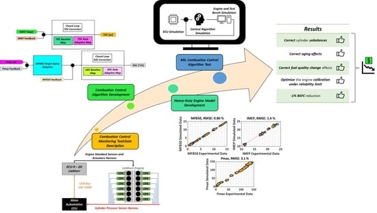
Enhancement of Heavy-Duty Engines Performance and Reliability Using Cylinder Pressure Information


Department of Industrial Engineering, University of Bologna, Viale Risorgimento, 2, 40136 Bologna, Italy
*
Author to whom correspondence should be addressed.
Energies 2023, 16(3), 1193; https://doi.org/10.3390/en16031193
Submission received: 23 December 2022
/
Revised: 13 January 2023
/
Accepted: 17 January 2023
/
Published: 21 January 2023
(This article belongs to the Special Issue Experimental Investigation, Modeling and Optimization of Modern Internal Combustion Engines toward Their Sustainable Application in Future Road Mobility)
Abstract
:Sustainability issues are becoming increasingly prominent in applications requiring the use of heavy-duty engines. Therefore, it is important to cut the emissions and costs of such engines to reduce the carbon footprint and keep the operating expenses under control. Even if for some applications a battery electric equipment is introduced, the diesel-equipped machinery is still popular thanks to the longer operating range. In this field, the open pit mines are a good example. In fact, the Total Cost of Ownership (TCO) of the mining equipment is highly impacted by fuel consumption (engine efficiency) and reliability (service interval and engine life). The present work is focused on efficiency enhancements achievable through the application of a combustion control strategy based on the in-cylinder pressure information. The benefits are mainly due to two factors. First, the negative effects of injectors aging can be compensated. Second, cylindrical online calibration of the control parameters enables the combustion system optimization. The article is divided into two parts. The first part describes the toolchain that is designed for the real-time application of the combustion control system, while the second part concerns the algorithm that would be implemented on the Engine Control Unit (ECU) to leverage the in-cylinder pressure information. The assessment of the potential benefits and feasibility of the combustion control algorithm is carried out in a Software in the Loop (SiL) environment, simulating both the developed control strategy and the engine behavior (Liebherr D98). Our goal is to validate the control algorithm through SiL simulations. The results of the validation process demonstrate the effectiveness of the control strategy: firstly, cylinder disparity on IMEP (+/−2.5% in reference conditions) is virtually canceled. Secondly, MFB50 is individually optimized, equalizing Pmax among the cylinders (+/−4% for the standard calibration) without exceeding the reliability threshold. In addition to this, BSFC is reduced by 1% thanks to the accurate cylinder-by-cylinder calibration. Finally, aging effects or fuel variations can be implicitly compensated, keeping optimal performance thorough the engine life.
1. Introduction
In many areas, such as the automotive industry, regulations lowered CO2 emission limits to push manufacturers and OEMs toward more efficient technologies with a reduced environmental impact [1,2]. At the same time, the market of heavy-duty vehicles in Europe is being addressed by the introduction of the 2019/1242 regulation [3].
So far, this trend had a limited impact on the research of heavy-duty, off-road engines. In the mining industry, the amount of CO2 emissions due to engine inefficiency is relatively low if compared to the effect of the fugitive methane [4]. However, even in the mining field, the efforts are directed to increasing the equipment/operation efficiency, resulting in a lower energy consumption (electricity/fuel) to address both the environmental and economic sustainability of mining operations, reducing the Greenhouse Gas (GHG) emissions and the extraction costs. The same considerations apply to other industrial fields (railway, maritime, genset) where heavy-duty diesel engines are still largely used.
In the literature, one of the most common approaches proposed to increase the mining operation efficiency is the automation of the entire process [5,6,7]. Furthermore, it could be convenient to switch from diesel engine to completely electric mining equipment [8,9,10,11] to ease the automation of mining operations, especially in applications where the use of completely electric machinery is considered feasible (underground mining). The major advantages of such approach to the mining industry are the following [5,8]:
- Reduction in costs, energy consumption and emissions;
- Increase in workplace safety; and
- Increase in workplace air quality, especially in underground mining.
However, in several applications, the use of internal combustion engines cannot be efficiently replaced. For example, in the open pit mines, the complete electrification of the vehicles is difficult, because the layout of the mine is always changing. In fact, for this application, the use of hybrid systems, that could improve the performance of traditional diesel machinery, looks easier to be implemented [8,9,10,11,12,13]. Diesel engines provide [8] longer operating range, higher specific energy (~12 kWh/kg), lower capital cost [14] and faster refueling compared to full electric powertrains [15]. For this reason, diesel engines remain an important part of the vehicle. Therefore, it is crucial to continue the development of ICEs to increase their efficiency and reduce fuel consumption, GHG emissions and the cost of the mining machinery.
The mine production strongly depends on the proper operation of the mining equipment and its reliability [16]. This aspect is even more crucial in automated mines; thus, the maintenance of the equipment is crucial to avoid expensive downtime or critical failures.
Monitoring the state of health of heavy-duty machinery also reduces fuel consumption; some examples can be found in [17].
The most common maintenance approaches are reported below [16]:
- Planned preventive maintenance [21];
While breakdown maintenance is often unacceptable, due to unpredictable plant shutdown, scheduled maintenance of heavy-duty engines is the most common solution. It may involve the replacement of fluids and spare parts (oil, coolant, filters) but also the mechanical and electro-mechanical components. During scheduled maintenance, some parts may be unnecessarily replaced, increasing the TCO.
Several examples of condition monitoring methods applied to diesel engines can be found in the literature. For light and medium-duty engines, the need for cost reduction pushes toward solutions based on low-cost or virtual sensors [25,26], which also allow the estimation of the engine-out emissions [27] and the combustion indexes [28,29,30] or predicting failures [29]. All these approaches are becoming increasingly common thanks to the increase in digitalization [5,29] and the advanced data analysis made available by the cloud technologies [16]. Better results, however, can be obtained by monitoring the combustion process using the in-cylinder pressure information. Both indirect [30] and direct [31,32] sensing is achievable, and the latter guarantees better accuracy. The efficiency increase for a production heavy-duty engine by means of a proper combustion control system needs an accurate evaluation of the combustion indexes, which is also useful for the implementation of predictive maintenance strategies [33]. The increased purchasing costs can be easily over-compensated by savings in fuel consumption and reducing the maintenance cost.
In the context of condition monitoring, a new system is being developed at Liebherr Components Colmar to enhance the performance and reliability of diesel engines. This system is based on the direct measurement of in-cylinder pressure. The objective of such a system is twofold:
- To evaluate significant combustion metrics (MFB50, IMEP, Pmax, etc.) starting from the pressure measurement and to compensate aging effects and disparities in the components behavior by using such metrics as inputs for a feedback control system, thus enhancing engine performance;
- To evaluate the engine health, thus determining the best time for the component substitution. Usually, the engine parts (pistons, injectors, cylinder heads, etc.) are replaced after a priori fixed time, often resulting in unnecessary costs due to the substitution of healthy components [34].
In this way, it is possible to increase efficiency and reliability, extending the equipment’s operating life. Furthermore, by providing combustion indexes to the ECU, it is possible to make the engine unsensitive to the type of fuel used. Using such an approach, the ECU can adapt the fuel delivery to the current condition, ensuring that specific targets based on the combustion metrics are met, regardless of the quality of the fuel used. This is another great advantage of such a system, since the use of alternative fuels (biofuels [35,36], hydrogen [37,38], fuel blends [39,40]) is expected to increase.
The authors have experimentally demonstrated in [41] the potential advantages of a combustion analysis system based on cylinder pressure sensors and a dedicated combustion control unit.
The present work describes in detail the toolchain that is being developed, showing how it can be used to control the combustion process, mitigating the cylindrical disparity, aging and other undesired effects. The mentioned controller is coupled to the model of the Liebherr D98 engine, and some simulations are executed in an SiL environment. The result of such simulations highlights the accuracy and the robustness of the developed controller, showing its impact on the main combustion metrics (IMEP, MFB50 and Pmax) and specific fuel consumption. The paper is focused on the control structure, and it does not investigate the definition of the targets and thresholds.
2. Experimental Setup
The Combustion Control Monitoring toolchain developed at Liebherr Components Colmar is composed by three parts, as shown in Figure 1:
- Cylinder Pressure Sensors (CPS);
- Combustion Control Unit (CCU);
- Engine Control Unit (ECU, Liebherr H-2D Unit [42]).
The combustion control system developed in this work is based on the signal obtained by in-cylinder pressure sensors.
The engine considered for the experimental campaign is equipped with cylinder heads with direct access to the combustion chamber by means of threaded connections, and no further modifications have been implemented. Thus, the use of such a toolchain for standard production engines is straightforward. Several types of sensors have been tested (both piezoelectric and piezoresistive), and the CCU can be easily adapted to the voltage-based (+/−10V) or current-based (4–20 mA) sensor output.
The main characteristics of the Liebherr engine considered for this activity are available in [43]. The Combustion Control Unit (developed by Alma Automotive) is based on the Miracle 2 platform [44], and it acquires and processes the signals coming from all the cylinders, complying with the specific standard of robustness and reliability needed for mining applications. Its compact and rugged design makes it suitable for on-board heavy-duty applications.
The last part of the LCCM toolchain is the Liebherr Engine Control Unit ECU2-HD [42]. This device is completely designed and manufactured inside Liebherr to optimize the control of diesel and stationary gas engines. The ECU2-HD is fully compatible with the Liebherr Common Rail System, and it can control all the engine functions as well as the Liebherr SCR system with the Ad-Blue dosing.
In the toolchain here described, the engine control unit (ECU2-HD) has the objective of analyzing the combustion indexes communicated by the CCU via CAN, using this information to achieve two main goals. First, the system should use combustion metrics to maximize the engine performance through the pressure-based feedback control. Then, it should help diagnosing potential mechanical issues that could happen during the engine operation, easing and speeding up the maintenance operations.
The following sections describe the feedback controller. The combustion metrics evaluated by the CCU (MFB50, IMEP and Pmax) are compared with the setpoints calibrated in the ECU, which sets the injectors actuations (Start Of Current, SOC and Time Of Current, TOC) to meet the target. The achievable performance enhancement related to the use of the combustion controller are due to:
- A more efficient calibration of the injection actuations (no need for safety margins at the expense of engine efficiency);
- The sensitivity of the performance to the fuel is minimized;
- The ECU can compensate the performance loss originated by components aging or production disparities.
3. Development and Validation of the Controller
This section focuses on the description of the combustion controller structure, the engine model, and the results achievable by using the suggested combustion control approach.
3.1. Control Algorithm
The algorithm proposed hereafter complies with two main objectives:
- Balancing the cylindrical variation of the indicated torque (so to achieve even cylinders wear, thus maximizing the service period);
- Compensating undesired effects such as the components aging, production disparities and variations in fuel quality.
Furthermore, the proposed combustion controller must be compatible with the speed-control function already implemented in the Liebherr ECU2-HD. For this reason, the developed algorithm is characterized by a simple structure (shown in Figure 2) and relies on the definition of the load index (fuel mass to be injected) used for other ECU functions. The function inside the Pre-Control block is already implemented in the ECU2-HD, and it defines the injected fuel mass as a function of the engine speed and pedal request.
The combustion metrics considered as the most important for the development of the control strategy are listed below:
- IMEP (Indicating Mean Effective Pressure), which is related to engine torque;
- MFB50 (50% of Mass Fraction Burnt), which is strictly related to engine efficiency (BSFC);
- Pmax (peak cylinder pressure), which should not exceed a tolerable threshold, to guarantee the engine reliability.
IMEP is used to determine the injection duration (TOC). The TOC of the injectors will be individually controlled to reach a specific value of IMEP for all the cylinders.
MFB50 and Pmax are used for the definition of the injection start angle (SOC): the SOC of the injectors is used as a control lever to individually reach the target value of MFB50. Pmax, instead, is used to set a lower bound for MFB50, preventing the use of SOC settings that would lead to exceeding the maximum tolerable pressure peak.
3.1.1. Definition of TOC
The time of current is calculated by the ECU as:
The TOC is evaluated as the sum of the feed-forward portion and the correction component, and the latter is evaluated by means of a PID controller. Figure 3 shows the block diagram referring to the definition of the feed-forward contribution.
The feed-forward TOC ( is defined using two lookup tables (LUTs). The first one is the Calibration Map of the Injectors, which is representative of the average injector behavior. The ECU gathers rail pressure via direct measurements, while the quantity of fuel to be injected is determined through a dedicated lookup table, depending on the operating conditions. In this way, the ECU estimates the base injector opening time to inject the correct amount of fuel inside the combustion chamber.
The TOC value determined using the base injector calibration map is then corrected using the individual-cylinder LUTs. The correction depends on two inputs: the engine speed and load indexes. These correction maps are used to compensate for disparities between the injectors due to production differences and the effect of pressure waves within the high-pressure rail [45].
The feed-forward model does not require the signal of the in-cylinder pressure sensors (correction maps could be set up once for all at the test bench). The combustion process insight is crucial for the introduction of a self-adaptive strategy, which allows compensating unwanted effects due to the components aging and fuel quality variations.
As described in Equation (1), the feed-forward value of the TOC is adjusted for each cylinder (. The TOC correction is made by a PID controller. The PID uses feedback signals from the CCU to correct the feed-forward TOC, so that a specific IMEP target value is reached. The value of the target IMEP is defined by the ECU using a LUT, which is accessed through indexes representing the operating condition (engine speed and load).
Since the target IMEP is the same for all the cylinders, a PID controller can be used to balance the fuel introduction, so that IMEP (i.e., torque) production is evenly distributed across the engine, despite variations in the injector performance that could occur due to aging, production disparities or pressure waves effect. The injectors’ performance variations are usually compensated using the correction map described in the feed-forward block. These maps can be filled with a proper calibration, requiring time-consuming tests, since for each cylinder, a correction factor must be determined for the entire operating range. Using the LCCM system, instead, the ECU can rely on the combustion feedback, so that the PID controllers continuously determine the proper factor forcing all the injectors to introduce the amount of fuel producing the target IMEP. To exploit this feature, an auto-adaptive block (see Figure 4) is implemented.
The block is activated only under appropriate conditions:
- Constant driver requests (pedal);
- Engine is warmed up;
- Steady-state conditions;
- Absence of faults.
When the activating conditions are met, the block updates the correction values of the feed-forward component with the current PID outputs [46]. The PID controllers are then reset and restarted.
Thanks to the adaptability of this algorithm, it is possible to continuously update the engine calibration and correct undesired effects originated by the components aging or changes in the fuel quality.
3.1.2. Definition of SOC
The definition of SOC follows the same approach described above for the computation of TOC. Indeed, as sketched out in Figure 5, this parameter is determined as the sum of a feed-forward contribution and a closed-loop correction:
As for the TOC, the feed-forward part of the SOC (), too, is the sum of two contributions. Both depend on the engine working point. The ECU uses the engine speed and load index information to estimate the base value of the SOC, which is then modified via individual cylinder corrections depending on the same inputs. The SOC base map is determined once, and it is the same for all the cylinders.
Similarly, the feed-forward value of the SOC is corrected with the same approach used for the TOC: a cylinder-individual PID controller feeds an auto adaptive block that, when enabled, uses the integral part to fill the individual correction maps present in the feed-forward block. The PID modifies the SOC to achieve a specific MFB50 target value. Figure 6 shows the structure of the SOC controller.
3.1.3. Definition of MFB50 Target
The MFB50 target value is defined by the ECU cylinder by cylinder using the algorithm reported in Figure 7. Two lookup tables are queried using the engine operating point (defined by a particular couple of the engine speed and load values). For each cylinder, the target MFB50 is determined as the higher value between the outputs of the two LUTs.
The first matrix (Optimum Map) collects the MFB50 values that make the engine run with the minimum specific fuel consumption, while the second map (Limit Map) collects the MFB50 limit (minimum) values that a specific cylinder can tolerate. Figure 8 and Figure 9 allow understanding the different meanings of the LUTs. For confidentiality reasons, all the figures reported hereinafter show normalized combustion indexes. IMEP, Pmax and MFB50 have been plotted subtracting an arbitrary offset value, while BSFC is represented as a percentage of the first measured value during the test.
Data displayed in Figure 8a,b are collected with a SOC sweep test described in [41]. During this test, the engine is operated under steady-state conditions, while TOC and SOC are manually modified to achieve a constant IMEP with different settings of the combustion phase for all twelve cylinders. Figure 8a shows that BSFC, i.e., engine efficiency, is influenced by the MFB50 average value. The optimal setting may change according to the running condition [47], but it is unlikely to change from cylinder to cylinder; thus. the first LUT collects MFB50 optimal values of the given engine over the engine operating range. Figure 8b shows that Pmax is related to MFB50, too. Within the engine maximum efficiency range, the lower the MFB50, the higher the Pmax. When the MFB50 is widely higher than the optimal value, the trend is flipped due to the increased exhaust gas temperature, which causes higher boost pressure and finally higher in-cylinder pressure at the end of the compression phase (when the combustion process is over-delayed, the pressure peak is reached at the end of the compression stroke).
Figure 8a shows that the value of the normalized MFB50 minimizing BSFC is lower than 3 °CA (this evaluation, however, is not accurate, being derived from the extrapolation of the experimental results). Each cylinder should be ideally operated with the optimal value of the combustion phase. Figure 8b shows why this is not possible. As already mentioned, when MFB50 decreases, the pressure peak rapidly rises. Interestingly, it is possible to see that the two cylinders reach the maximum tolerable pressure peak (i.e., reliability limit) for different values of MFB50 (4.4 °CA for cylinder 1 and 5.4 °CA for cylinder 6), so it makes sense to consider this trend individually, with dedicated cylinder LUTs. Other limiting factors, such as NOx emissions, could be considered.
To sum up, in the tested operating point (1800 rpm and 22 bar of BMEP), the two cylinders share the same MFB50 optimum value:
On the contrary, the two cylinders have different threshold values:
As already remarked for the figures, also, the optimal and threshold values reported in Equations (3)–(5) have been scaled for confidentiality reasons.
The previous example explains why it would be of interest to make all the cylinders work with the optimal combustion phasing to achieve the best engine efficiency (i.e., the minimum fuel consumption) and why it is not always possible due to reliability issues. Furthermore, from Figure 8a,b, one can appreciate that while the optimal MFB50 value is the same for all the cylinders, the MFB50 threshold value can be different for each cylinder.
The MFB50 optimal value depends on the trade-off between the excessive heat and pumping losses (over-advanced combustion) and energy conversion inefficiencies (over-delayed combustion) [47]; thus, it is essentially constant throughout the engine’s life, while the MFB50 limit for a given cylinder is expected to change with the passing of time. In fact, due to aging, the cylinders tend to decrease their performance, as shown in Figure 9. In particular, the piston rings’ wear produces an increase in the cylinder blow-by that has the same effect of a compression ratio reduction.
This means that the same MFB50 setting would lead to lower peak pressures. Therefore, advancing the MFB50 Limit Map values, it would be possible to partially recover the performance loss due to aging. For this reason, in the proposed control approach, the MFB50 target for all the cylinders is determined as the higher between optimal and limit values, the latter being continuously adapted cylinder by cylinder to the actual state of health of the engine.
When appropriate conditions are met, the adaptation strategy for the MFB50 does not follow the logic presented in the default state (Figure 7) but rather that illustrated in Figure 10.
The adaptation strategy for the MFB50 Limit Map is activated when the engine is warmed up and it is running under steady-state conditions, and finally, the engine is either in an “aging correction state” or “reliability correction state”.
The “aging correction state” is defined by the following additional conditions:
- The value of the cylinder MFB50 currently measured is greater than optimum;
- The feedback value of the Pmax is lower than the acceptable limit.
- The “reliability correction state” is defined by the following additional conditions:
- The feedback Pmax value is greater than the acceptable limit;
The MFB50 measured for a given cylinder is greater than the optimum.
Once the conditions for activating the adaptation strategy of MFB50 have been reached, cylinder individual PID controllers lead to specific MFB50 target setpoints, keeping the Pmax at the limit value for all the cylinders. The MFB50 value that allows to reach the Pmax limit is then stored in the MFB50 Limit Map of the corresponding cylinder.
The Pmax limit value is determined by the ECU using an LUT, according to the engine operating point. This map is defined during the calibration process, and it is the same for all the cylinders.
3.2. Model in the Loop Simulations Approach
The model in the Loop (MiL) simulations have been used to test the proposed combustion control algorithm. An engine model has been used to generate the combustion metrics data flow feeding the combustion control algorithm. The model simulates the engine’s behavior in a test bench environment; thus, the current engine speed is determined by the engine and brake torque equilibrium, considering respective inertias. Figure 11 sketches the main blocks of the Simulink model used for MiL simulations.
The Simulink model consists of five main blocks:
- ECU Base Actuations: Base actuations and setpoints are calculated according to the engine speed and pedal request, using lookup tables.
- Combustion Controller: The control strategies described in Section 3 are implemented in this block.
- Engine Model: The engine is represented in terms of combustion metrics flow: the accuracy in representing the main combustion metrics is reported in Table 1. For a realistic data flow representation, cycle-to-cycle variations are statistically described, considering the standard deviation of MFB50. In details, the model can be described by the following equations:
- Minj represents the mass of fuel injected in the cylinder;
- Pmot is the peak pressure inside the cylinder without combustion (motoring pressure);
- Pboost indicates the air pressure after the compressor;
- rc is the volumetric compression ratio; and
- γ is the ratio of the specific heats (constant pressure and the constant volume).
- 4.
- Torque Equilibrium: As already remarked, engine speed is determined solving the torque equilibrium equation:
- Te is the engine torque, which is calculated thanks to the IMEP of the twelve cylinders and the engine friction information, stored in an LUT;
- Tl is the load torque produced by the electric brake;
- Ie represents the engine inertia;
- Il represents the electric motor inertia; and
- ꙍ is the engine speed expressed in rad/s.
Inverting the equation 10 it is possible to calculate the engine speed:
- 5.
- Test Bench Electric Brake: The braking torque produced by the electric brake is achieved by means of a PID controller, which is fed with target speed and actual speed.
Equations (6)–(9) have been defined and validated for the whole engine operating range covered during a truck cycle, i.e., 1300–1800 rpm and 20–100% engine load.
4. Results and Discussion
All the results presented in this section refer to simulations carried out with the engine working at a constant speed of 1800 rpm and a steady pedal request of 100%. The only differences in the simulations are related to the control actions, which change according to the type of control activated for the given simulation.
The conditions that will be described are:
- Standard Engine Calibration: It is the reference condition, and the engine control unit uses only the standard calibration, and all the feedback controls are deactivated.
- Only PI Controller: The engine is working using only the PI controller following the MFB50 and IMEP target values.
- PI Controller and Auto Adaptation: The engine is working with the PI and the full auto adaptation strategy (SOC, TOC and MFB50 threshold) activated.
Figure 12, Figure 13 and Figure 14 compare the combustion metrics achieved under the reference condition with those obtained activating the PI controllers on SOC and TOC. Once again, it can be useful to recall that the reported combustion metrics have been normalized.
As expected, Figure 12a,b show that when the PI controllers are active, it is possible to properly correct the cylinder IMEP unbalance. In fact, when the controllers are active, the IMEP produced by all cylinders lays within ±0.3% of the desired target value. As a result, thermal and mechanical stress is evenly distributed among the cylinders.
Figure 13a,b show the effect of the combustion controller activation on MFB50. Both figures report the values of the normalized MFB50 optimal (7.7 °CA) and threshold (11.7 °CA) values for all the cylinders. For this initial step of the simulation, all the twelve cylinders share the same minimum MFB50 limit: as Figure 13a shows, the standard calibration setting leads to lower MFB50 values, which means that once the control on MFB50 is activated, SOC will be delayed for all the cylinders. As a result, MFB50 scatters are grouped around the threshold, as seen in Figure 13b. Furthermore, the threshold value used was deliberately more conservative than necessary to emphasize the restraining action of the controller: the simulated scenario corresponds to an over-conservative setting (excessively high value) of MFB50 threshold, which will lead to peak pressures lower than the acceptable boundary.
Leaving aside the minimum MFB50 threshold setting, when the PI controllers are active, the cylinder MFB50 unbalance is properly corrected, and the MFB50 feedback value is within ±0.15 °CA of the target. Since the optimal MFB50 is lower than the minimum allowable value, the target of the PID in this simulation matches the MFB50 threshold.
Figure 14a,b compare the values of normalized Pmax assumed by the twelve cylinders with the two different control settings. Figure 14a reveals that the reference condition is marked by a significant unevenness of Pmax within cylinders: the average normalized Pmax over the cylinders within 200 cycles is 125.6 bar, while the minimum and maximum values are 121 bar (cylinder 3) and 130 bar (cylinder 1), respectively. As the PI controllers are activated (Figure 14b), normalized Pmax values of the twelve cylinders are grouped, since all the cylinders are managed using the same MFB50. However, a certain degree of dispersion remains due to the differences between cylinders. As shown in Figure 10, the cylinder pressure at the end of the compression phase could be different, which would deliver different peak pressures with the same MFB50. Furthermore, the fuel delivery may be slightly different for each cylinder, leading to longer or shorter combustion durations, impacting the Pmax. The average normalized Pmax over the cylinders within 200 cycles produced by the twelve cylinders is 119 bar, and the extreme values are 122 bar (produced by cylinder 10) and 116 bar (produced by cylinder 11).
Pmax values appreciably decrease when PI controllers are active compared to the reference condition, because, as already remarked, simulation has been run using a very conservative MFB50 threshold value. In fact, from Figure 14b, it is also possible to appreciate that the average Pmax produced by the twelve cylinders is considerably lower compared to the cylinder maximum tolerable Pmax threshold. In this condition, where the combustion is too retarded, engine efficiency can be increased by advancing the combustion phase for all the cylinders, leading Pmax values to the threshold limit. This correction of the MFB50 threshold value is produced by the auto adaptation strategy of the combustion phase described above.
Figure 15 shows the normalized combustion metrics behavior when the PI controllers and all the auto adaptation strategies (SOC, TOC and MFB50 threshold) are activated. Comparing Figure 12a,b, it is possible to appreciate that with the learning of the ΔTOC corrections, all the cylinders produce an IMEP closer to the target (±0.15% of the target value): the auto-adaptation strategies limit the PID action, improving overall accuracy.
Figure 15b shows that in this case, not only the IMEP but also the Pmax produced by all the cylinders are phased around the targets. In fact, activating all the auto-adaptation strategies, individual MFB50s are set to match the maximum pressure threshold. With the adaptation of the MFB50 threshold, all the cylinders are producing peak pressures within ±1 bar of the limit value. The controller automatically defines for each cylinder a new MFB50 threshold value. Figure 15c,d represent the new cylinder MFB50 thresholds.
The following figure reports the behavior of the normalized combustion metrics (IMEP, MFB50 and Pmax) produced by the twelve cylinders during a step-by-step activation of the combustion controller strategies. In the three plots, the time of the controller activation is highlighted. The yellow line indicates the moment when the PI controllers for the TOC and SOC are triggered. The green line represents the time when the auto-adaptation strategies for the ΔTOC and the ΔSOC corrections are activated. Finally, the blue line indicates when the adaptation of the MFB50 threshold value is switched on.
The IMEP feedback and target values are superimposed in 16 (a): it is evident that the only significant variation occurs at around 200 s, when the PI controllers are activated. In fact, starting from this instant, the PI controller adjusts the injections time (TOC), producing the desired IMEP after 9 s. From this moment onward, the IMEP produced by the cylinders is always close to the desired target, regardless of which auto-adaptation strategy is activated.
Figure 16b,c show the behavior of the normalized MFB50 and Pmax, respectively. From the instant t = 200 s, when the SOC PI controllers are activated, the system can adjust the SOC actuation, converging to the MFB50 threshold initially set. From this moment onward, the cylinder produces the desired MFB50 until the auto-adaptation strategy for the ΔTOC and ΔSOC are activated (t = 400 s). The correction is then gradually learnt by the controller, and the feed-forward value of the SOC (see Figure 11) is progressively modified. Until 600 s, the target combustion phase is sub-optimal, sticking to the initial threshold. This setting, however, produces a value of Pmax significantly lower than the acceptable limit (Figure 16c). For this reason, when the adaptation strategy on the combustion phase is activated at 600 s, the controller modifies the MFB50 threshold value on each cylinder until Pmax reaches the threshold limit. This behavior is also confirmed by Figure 16c, where it is evident how the controller, after 600 s, can bring the feedback closer to the desired Pmax value in 75 s, decreasing the MFB50 lower threshold for each cylinder.
Figure 17 shows the impact of the control strategies on the BSFC. Once the SOC and TOC PI controllers are activated (t = 200 s), the BSFC increases, because as shown in Figure 16b, the MFB50 target is far from optimum. In fact, when the MFB50 target adaptation strategy is activated (t = 600 s) the BSFC starts decreasing. Indeed, since at 600 s, peak pressures of all cylinders are lower than the limit, the MFB50 target can be pushed toward the optimal setting.
Using auto-adaptive strategies of SOC and TOC improves steady-state control quality and transient behavior as well. In the following figures, a different type of comparison between the “Open Loop before SOC and TOC adaptation” and the “Open Loop after SOC and TOC adaptation” sequences is carried out. In particular, the results achieved in terms of distance of IMEP and MFB50 from the targets, before and after the adaptation of SOC and TOC were analyzed, over a small portion of the truck cycle described in [41]. The test conditions are shown in Figure 18.
In Figure 19b–d and Figure 20b–d, the error is calculated as the difference between the target and the measured values. The graphs in Figure 19 and Figure 20 show that the auto-adaptation strategies on TOC and on SOC can compensate the undesired effects due to aging or cylinder disparity not only under steady-state conditions but also under transient conditions. In fact, while the IMEP error before the adaptation of TOC is between −0.63 bar and +1.2 bar, after the adaptation, it is within ±0.08 bar. The same can be said for the MFB50, where the error variation range decreases from 2.6 °CA, before the SOC adaptation, to 0.8 °CA after the SOC adaptation.
5. Conclusions
This work assesses the potential benefits achievable with a closed-loop combustion control system based on the measurement of the in-cylinder pressure. The main advantages, in terms of engine efficiency, are related to the possibility to follow the components’ aging, fuel quality variations, calibration inaccuracies, and production disparities. Other benefits come from the balancing of the mechanical and thermal stresses on the engine components, and this reduces the maintenance effort.
The paper shows that using a proper feedback combustion control algorithm, it is possible to maximize the engine performance without affecting the reliability. The SiL simulations demonstrate that the combustion controller can balance the cylinders performance, controlling the combustion phase of each cylinder to keep it close to the maximum efficiency value. On one hand, the PI controllers keep the IMEP and Pmax of all the cylinders close to the same value, improving the uniformity of the components wear. On the other hand, the auto-adaption strategies on TOC and SOC adjust the injectors actuations to compensate the effects of the components’ aging and production disparities (each injector has a different calibration map).
Finally, the combustion controller shows the capability to enhance the engine efficiency (i.e., reducing the specific fuel consumption) by modifying the standard engine calibration. The combustion controller optimizes the minimum admissible value of MFB50 for each cylinder, compensating the effects related to an over-conservative engine calibration, or cylinders’ aging. The same strategy could be used for components’ protection.
The results achieved with the durability test presented in [41] and the simulation of the combustion controller demonstrate the feasibility of the on-board application of the presented Combustion Control Monitoring toolchain.
The described activity is going on at Liebherr with the implementation of the cylinder pressure-based combustion control system on standard ECUs and mounting instrumented heads on the tested engines.
Author Contributions
Conceptualization, E.C. and A.R.; methodology, E.C. and A.R.; software, A.R.; validation, E.C., A.B. and D.M.; formal analysis, D.M. and A.B.; investigation, A.B. and D.M.; resources, E.C.; data curation, E.C. and A.R.; writing—original draft preparation, A.R.; writing—review and editing, E.C.; visualization, A.R.; supervision, E.C.; project administration, E.C.; funding acquisition, E.C. All authors have read and agreed to the published version of the manuscript.
Funding
This research received no external funding.
Institutional Review Board Statement
not applicable.
Informed Consent Statement
Informed consent was obtained from all subjects involved in the study.
Data Availability Statement
3rd Party Data.
Acknowledgments
The authors would like to thank Francois Rey and all the staff at Liebherr Colmar SaS making this work possible.
Conflicts of Interest
The authors declare no conflict of interest.
Nomenclature
| BMEP | Brake Mean Effective Pressure |
| BSFC | Brake Specific Fuel Consumption |
| CAN | Controller Area Network |
| CCU | Combustion Control Unit |
| COC | Components of Colmar |
| CO2 | Carbon Dioxide |
| CPS | Cylinder Pressure Sensor |
| ECU | Engine Control Unit |
| GHG | Greenhouse Gases |
| Hil | Hardware In the Loop |
| Ie | Engine Inertia |
| Il | Electric Brake Inertia |
| ICE | Internal Combustion Engines |
| IMEP | Indicated Mean Effective Pressure |
| LCCM | Liebherr Combustion Control Monitoring |
| LUT | Lookup Table |
| MFB50 | Crankshaft angle corresponding to 50% of the mass fraction burnt |
| MFB50opt | Optimum value of 50% of the mass fraction burnt |
| MFB50thr | Threshold of 50% of the mass fraction burnt |
| Mil | Model In the Loop |
| Minj | Fuel Injected Mass |
| NOx | Nitrogen Oxides |
| OEM | Original Equipment Manufacturer |
| PI | Proportional Integrative Controller |
| PID | Proportional Integrative Derivative Controller |
| Pboost | Air Pressure after the compressor |
| Pmax | Maximum Peak Pressure reached inside the combustion chamber |
| Pmot | Motoring Pressure |
| RMSE | Root Mean Squared Error |
| Sil | Software in the Loop |
| SCR | Selective Catalyst Reduction |
| SOC | Start of Current |
| SOCFF | Start of Current Feed Forward |
| TCO | Total Cost of Ownership |
| TOC | Time of Current |
| TOCFF | Time of Current Feed Forward |
| Te | Engine Torque |
| Tl | Load Torque |
| rc | Compression Ratio |
| t | Time |
| ∆SOC | Variation of Start of Current |
| ∆SOCcyl# | Variation of Start of Current different from cylinder to cylinder |
| ∆TOC | Variation of Time of Current |
| ∆TOCcyl# | Variation of Time of Current different from cylinder to cylinder |
| γ | Ratio between the specific heat at constant pressure and the specific heat at constant volume |
| ꙍ | Engine Speed in rad/s |
| °CA | Crank Angle Degree |
References
- Monteiro, N.B.R.; da Silva, E.A.; Neto, J.M.M. Sustainable development goals in mining. J. Clean. Prod. 2019, 228, 509–520. [Google Scholar] [CrossRef]
- DieselNet. Emission Standards: Summary of Worldwide Engine and Vehicle Emission Standards. DieselNet. Available online: https://dieselnet.com/standards/ (accessed on 1 May 2021).
- EUR-Lex. Regulation (EU) 2019/1242 of the European Parliament and of the Council of 20 June 2019 Setting CO2 Emission Performance Standards for New Heavy-Duty Vehicles and Amending Regulations (EC) No 595/2009 and (EU) 2018/956 of the European Parliament and of the Council and Council Directive 96/53/EC. European Union. Available online: https://eur-lex.europa.eu/eli/reg/2019/1242/oj (accessed on 1 May 2021).
- McKinsey Sustainability. Climate Risk and Decarbonization: What Every Mining CEO Needs to Know. McKinsey Sustainability. Available online: https://www.mckinsey.com/business-functions/sustainability/our-insights/climate-risk-and-decarbonization-what-every-mining-ceo-needs-to-know (accessed on 1 May 2021).
- MiningMagazine, The Benefits of Predictive and Prescriptive Maintenance in Mine Autonomy. Available online: https://www.miningmagazine.com/partners/partner-content/1396266/the-benefits-of-predictive-and-prescriptive-maintenance-in-mine-autonomy (accessed on 1 May 2021).
- Rogers, W.P.; Kahraman, M.M.; Drews, F.A.; Powell, K.; Haight, J.M.; Wang, Y.; Baxla, K.; Sobalkar, M. Automation in the Mining Industry: Review of Technology, Systems, Human Factors, and Political Risk. Min. Met. Explor. 2019, 36, 607–631. [Google Scholar] [CrossRef]
- Ralston, J.; Reid, D.; Hargrave, C.; Hainsworth, D. Sensing for advancing mining automation capability: A review of underground automation technology development. Int. J. Min. Sci. Technol. 2014, 24, 305–310. [Google Scholar] [CrossRef]
- Ertugrul, N.; Kani, A.; Davies, M.; Sbarbaro, D.; Moran, L. Status of Mine Electrification and Future Potentials. In Proceedings of the 2020 International Conference on Smart Grids and Energy Systems (SGES), Perth, Australia, 23–26 November 2020; pp. 151–156. [Google Scholar] [CrossRef]
- Uno, K.; Imaie, K.; Eng, D.; Maekawa, K.; Smith, G.; Suyama, A.; Hatori, J. Development of Mining Machinery and Future Outlook for Electrification. Hitachi Rev. 2013, 62, 2. Available online: https://www.hitachi.com/rev/pdf/2013/r2013_02_102.pdf (accessed on 1 May 2021).
- Liebherr. Two New Local Zero Emission Excavators from Liebherr: R 976-E and R 980 SME-E Electric Crawler Excavators; Liebherr: Bulle, Switzerland, 2021; Available online: https://www.liebherr.com/en/ind/latest-news/news-press-releases/detail/two-new-local-zero-emission-excavators-from-liebherr-r-976-e-and-r-980-sme-e-electric-crawler-excavators.html (accessed on 1 May 2021).
- IVT International Industrial Vehicle Technology. Liebherr Truck with Overhead Line Projected to Save Mine Three Million Litres of Diesel a Year. IVT International Industrial Vehicle Technology. Available online: https://www.ivtinternational.com/news/mining/liebherr-truck-with-overhead-line-projected-to-save-mine-three-million-litres-of-diesel-a-year.html (accessed on 1 May 2021).
- Paraszczak, J.; Svedlund, E.; Fytas, K.; Laflamme, M. Electrification of Loaders and Trucks–A Step Towards More Sustainable Underground Mining. Renew. Energy Power Qual. J. 2014, 1, 81–86. [Google Scholar] [CrossRef]
- Abdel-baqi, O.; Nasiri, A.; Miller, P. Dynamic Performance Improvement and Peak Power Limiting Using Ultracapacitor Storage System for Hydraulic Mining Shovels. IEEE Trans. Ind. Electron. 2014, 62, 3173–3181. [Google Scholar] [CrossRef]
- Varaschin, J.; De Souza, E. Economics of diesel fleet replacement by electric mining equipment. In Proceedings of the 15th North American Mine VentilaHitachi Revtion Symposium, Blacksburg, VA, USA, 20–25 June 2015; IEEE: Washington, DC, USA, 2015; pp. 1–8. [Google Scholar]
- Cunanan, C.; Tran, M.-K.; Lee, Y.; Kwok, S.; Leung, V.; Fowler, M. A Review of Heavy-Duty Vehicle Powertrain Technologies: Diesel Engine Vehicles, Battery Electric Vehicles, and Hydrogen Fuel Cell Electric Vehicles. Clean Technol. 2021, 3, 474–489. [Google Scholar] [CrossRef]
- Kruczek, P.; Gomolla, N.; Hebda-Sobkowicz, J.; Michalak, A.; Śliwiński, P.; Wodecki, J.; Stefaniak, P.; Wyłomańska, A.; Zimroz, R. Predictive Maintenance of Mining Machines Using Advanced Data Analysis System Based on the Cloud Technology. In Proceedings of the 27th International Symposium on Mine Planning and Equipment Selection-MPES 2018; Springer: Cham, Switzerland, 2019. [Google Scholar] [CrossRef]
- Peralta, S.; Sasmito, A.P.; Kumral, M. Reliability effect on energy consumption and greenhouse gas emissions of mining hauling fleet towards sustainable mining. J. Sustain. Min. 2016, 15, 85–94. [Google Scholar] [CrossRef] [Green Version]
- Jardine, A.; Banjevic, D.; Wiseman, M.; Buck, S.; Joseph, T. Optimizing a mine haul truck wheel motors’ condition monitoring program. Use of proportional hazards modeling. J. Qual. Maintenance Eng. 2001, 7, 286–302. [Google Scholar] [CrossRef]
- Zimroz, R.; Wodecki, J.; Król, R.; Andrzejewski, M.; Sliwinski, P.; Stefaniak, P. Self-propelled mining machine monitoring system—Data validation, processing and analysis. In Mine Planning and Equipment Selection; Springer: Cham, Switzerland, 2014; pp. 1285–1294. [Google Scholar]
- Moczulski, W.; Szulim, R. On case-based control of dynamic industrial processes with the use of fuzzy representation. Eng. Appl. Artif. Intell. 2004, 17, 371–381. [Google Scholar] [CrossRef]
- Paolanti, M.; Romeo, L.; Felicetti, A.; Mancini, A.; Frontoni, E.; Loncarski, J. Machine Learning approach for Predictive Maintenance in Industry 4.0. In Proceedings of the 14th IEEE/ASME International Conference on Mechatronic and Embedded Systems and Applications (MESA), Oulu, Finland, 2–4 July 2018; pp. 1–6. [Google Scholar] [CrossRef]
- Mobley, R.K. An Introduction to Predictive Maintenance; Butterworth-Heinemann: Oxford, UK, 2002. [Google Scholar]
- Scheffer, C.; Girdhar, P. Practical Machinery Vibration Analysis and Predictive Maintenance; Elsevier: Amsterdam, The Netherlands, 2004. [Google Scholar]
- Garcia, M.C.; Sanz-Bobi, M.A.; del Pico, J. SIMAP intelligent system for predictive maintenance: Application to the health condition monitoring of a wind turbine gearbox. Comput. Ind. 2006, 57, 552–568. [Google Scholar] [CrossRef]
- Cavina, N.; De Cesare, M.; Ravaglioli, V.; De Ponti, F.; Covassin, F. Full Load Performance Optimization Based on Turbocharger Speed Evaluation via Acoustic Sensing. In Proceedings of the ASME 2014 Internal Combustion Engine Division Fall Technical Conference, Columbus, Indiana, 19–22 October 2014. [Google Scholar] [CrossRef]
- Ponti, F.; Ravaglioli, V.; Corti, E.; Moro, D.; De Cesare, M. Non-Intrusive Methodology for Estimation of Speed Fluctuations in Automotive Turbochargers under Unsteady Flow Conditions. SAE Int. J. Engines 2014, 7, 1414–1421. [Google Scholar] [CrossRef]
- Ponti, F.; Ravaglioli, V.; Moro, D.; De Cesare, M. Diesel Engine Acoustic Emission Analysis for Combustion Control; SAE Technical Papers; SAE International: Warrendale, PA, USA, 2012. [Google Scholar] [CrossRef]
- Ponti, F.; Ravaglioli, V.; Cavina, N.; De Cesare, M. Diesel Engine Combustion Sensing Methodology Based on Vibration Analysis. J. Eng. Gas Turbines Power 2013, 136, 111503. [Google Scholar] [CrossRef]
- Aqueveque, P.; Radrigan, L.; Pastene, F.; Morales, A.S.; Guerra, E. Data-Driven Condition Monitoring of Mining Mobile Machinery in Non-Stationary Operations Using Wireless Accelerometer Sensor Modules. IEEE Access 2021, 9, 17365–17381. [Google Scholar] [CrossRef]
- Scocozza, G.F.; Silvagni, G.; Brusa, A.; Cavina, N.; Ponti, F.; Ravaglioli, V.; De Cesare, M.; Panciroli, M.; Benedetti, C. Development and Validation of a Virtual Sensor for Estimating the Maximum in-Cylinder Pressure of SI and GCI Engines; SAE Technical Paper 2021-24-0026; SAE International: Warrendale, PA, USA, 2021. [Google Scholar] [CrossRef]
- Corti, E.; Raggini, L.; Rossi, A.; Brusa, A.; Solieri, L.; Corrigan, D.; Silvestri, N.; Cucchi, M. Application of Low-Cost Transducers for Indirect In-Cylinder Pressure Measurements. SAE Int. J. Engines 2022, 16, 18. [Google Scholar] [CrossRef]
- Willems, F. Is Cylinder Pressure-Based Control Required to Meet Future HD Legislation? IFAC-Pap. 2018, 51, 111–118. [Google Scholar] [CrossRef]
- Brusa, A.; Cavina, N.; Rojo, N.; Mecagni, J.; Corti, E.; Ravaglioli, V.; Cucchi, M.; Silvestri, N. Development and Experimental Validation of an Adaptive, Piston-Damage-Based Combustion Control System for SI Engines: Part 1—Evaluating Open-Loop Chain Performance. Energies 2021, 14, 5367. [Google Scholar] [CrossRef]
- You, M.-Y.; Liu, F.; Wang, W.; Meng, G. Statistically Planned and Individually Improved Predictive Maintenance Management for Continuously Monitored Degrading Systems. IEEE Trans. Reliab. 2010, 59, 744–753. [Google Scholar] [CrossRef]
- Dindarloo, S.R.; Siami-Irdemoosa, E. Determinants of fuel consumption in mining trucks. Energy 2016, 112, 240. [Google Scholar] [CrossRef]
- Menendez, J.; Loredo, J. Biomass production in surface mines: Renewable energy source for power plants. WSEAS Trans. Environ. Dev. 2018, 14, 205–211. [Google Scholar]
- Olavson, L.G.; Baker, N.R.; Lynch, F.E.; Mejia, L.C. Hydrogen Fuel for Underground Mining Machinery, SAE Transactions Vol. 93, Section 2: 840222––840402; SAE International: Warrendale, PA, USA, 1984; pp. 109–124. Available online: https://www.jstor.org/stable/44434233 (accessed on 1 May 2021).
- Guerra, C.F.; Reyes-Bozo, L.; Vyhmeister, E.; Caparrós, M.J.; Salazar, J.; Godoy-Faúndez, A.; Clemente-Jul, C.; Verastegui-Rayo, D. Viability analysis of underground mining machinery using green hydrogen as a fuel. Int. J. Hydrog. Energy 2020, 45, 5112–5121. [Google Scholar] [CrossRef]
- Reiter Aaron, J.; Kong, S. Combustion and emissions characteristics of compression-ignition engine using dual ammonia-diesel fuel. Fuel 2011, 90, 87–97. [Google Scholar] [CrossRef] [Green Version]
- Lesmana, H.; Zhang, Z.; Li, X.; Zhu, M.; Xu, W.; Zhang, D. NH3 as a Transport Fuel in Internal Combustion Engines: A Technical Review. ASME J. Energy Resour. Technol. 2019, 141, 070703. [Google Scholar] [CrossRef]
- Corti, E.; Raggini, L.; Rossi, A.; Brusa, A.; Moro, D. Investigation of Aging Effects on Combustion and Performance Characteristics of Mining Engines. SAE Int. J. Engines 2022, 16, 2023. [Google Scholar] [CrossRef]
- Liebherr. ECU2-HD Engine Control Unit. Liebherr. Available online: https://www.liebherr.com/en/aus/products/components/injection-systems/engine-control-units/details/ecu2hd.html (accessed on 1 October 2021).
- Liebherr. D9812 Dieselmotor. Liebherr. Available online: https://www.liebherr.com/en/int/products/components/combustion-engines/diesel-engines/product-portfolio-diesel-engines/details/d9812.html (accessed on 1 January 2023).
- Alma Automotive. OBI-M2 Combustion Analysis System. Alma Automotive. Available online: https://alma-automotive.it/products/obi-m2/ (accessed on 1 January 2020).
- Herfatmanesh, M.R.; Peng, Z.; Ihracska, A.; Lin, Y.; Lu, L.; Zhang, C. Characteristics of pressure wave in common rail fuel injection system of high-speed direct injection diesel engines. Adv. Mech. Eng. 2016, 8. [Google Scholar] [CrossRef]
- Poggio, L.; Ceccarini, D.; Gelmetti, A. A Method for Estimating the Stoichiometric Ratio for a Control System of an Internal Combustion Engine; European Patent Application: Munich, Germany, 2021.
- Eunhwan, K.; Jeongwon, S.; Jaesung, C.; Myoungho, S. Optimal Set-points Generation of MFB50 for Combustion Control in Diesel Engines. In Proceedings of the Paper presented at KSAE 2013 Annual Conference, Seoul, Republic of Korea, 21–23 October 2013. [Google Scholar]
Figure 1.
Schematics of the Liebherr Combustion Control Monitoring toolchain (LCCM).

Figure 2.
Connection between the pre-existing control (Pre-Control block) implemented inside the Liebherr ECU2-HD and the new control strategy (Combustion Control Block) based on the use of the combustion metrics.
Figure 2.
Connection between the pre-existing control (Pre-Control block) implemented inside the Liebherr ECU2-HD and the new control strategy (Combustion Control Block) based on the use of the combustion metrics.

Figure 3.
Schematic of the feed-forward model used for the definition of TOC.

Figure 4.
Block scheme of the closed loop part of the controller defining the correction component of the feed-forward TOC.
Figure 4.
Block scheme of the closed loop part of the controller defining the correction component of the feed-forward TOC.

Figure 5.
Schematic of the feed-forward model defining the base value of SOC.

Figure 6.
Schematic of the closed loop part of the controller defining the correction component of the feed-forward SOC.
Figure 6.
Schematic of the closed loop part of the controller defining the correction component of the feed-forward SOC.

Figure 7.
Block diagram for the determination of MFB50 target in the default state. During the learning state, the MFB50 target value for each cylinder is evaluated using the schematic in Figure 10.
Figure 7.
Block diagram for the determination of MFB50 target in the default state. During the learning state, the MFB50 target value for each cylinder is evaluated using the schematic in Figure 10.

Figure 8.
Trend of BSFC (a) and pressure peak (b) as a function of MFB50 for the working point 1800 rpm and 22 bar BMEP.
Figure 8.
Trend of BSFC (a) and pressure peak (b) as a function of MFB50 for the working point 1800 rpm and 22 bar BMEP.

Figure 9.
Example of compression ability loss expected from engine aging.

Figure 10.
Adaptation strategy used to update the MFB50 Limit Map.

Figure 11.
Schematic of Simulink control algorithm and the virtual model of the D98 engine.

Figure 12.
Comparison between the desired IMEP target and the actual value of IMEP produced by all the 12 cylinders at 1800 rpm and 100% pedal: (a) when the ECU is using only the open loop control, (b) when the PI control of SOC and TOC are active.
Figure 12.
Comparison between the desired IMEP target and the actual value of IMEP produced by all the 12 cylinders at 1800 rpm and 100% pedal: (a) when the ECU is using only the open loop control, (b) when the PI control of SOC and TOC are active.

Figure 13.
Comparison between the MFB50 optimum, threshold and actual values produced by all the 12 cylinders at 1800 rpm and 100% pedal: (a) when the ECU is using only the open loop control, (b) when the PI control of SOC and TOC are active.
Figure 13.
Comparison between the MFB50 optimum, threshold and actual values produced by all the 12 cylinders at 1800 rpm and 100% pedal: (a) when the ECU is using only the open loop control, (b) when the PI control of SOC and TOC are active.

Figure 14.
Comparison between the Pmax threshold, the Pmax limit and the actual values of Pmax produced by all 12 cylinders at 1800 rpm and 100% pedal: (a) when the ECU is using only the open loop control, (b) when the PI control of the SOC and TOC are active.
Figure 14.
Comparison between the Pmax threshold, the Pmax limit and the actual values of Pmax produced by all 12 cylinders at 1800 rpm and 100% pedal: (a) when the ECU is using only the open loop control, (b) when the PI control of the SOC and TOC are active.

Figure 15.
Comparison between desired and actual values of combustion metrics produced by all the 12 cylinders when all the strategies are active at 1800 rpm and 100% pedal: (a) IMEP, (b) Pmax, (c) MFB50 of cylinders 1–6, (d) MFB50 of cylinders 7–12.
Figure 15.
Comparison between desired and actual values of combustion metrics produced by all the 12 cylinders when all the strategies are active at 1800 rpm and 100% pedal: (a) IMEP, (b) Pmax, (c) MFB50 of cylinders 1–6, (d) MFB50 of cylinders 7–12.

Figure 16.
Behavior of the indicating variables feedback when the combustion controller strategies are activated in succession at 1800 rpm and 100% pedal: (a) IMEP, (b) MFB50, (c) Pmax.
Figure 16.
Behavior of the indicating variables feedback when the combustion controller strategies are activated in succession at 1800 rpm and 100% pedal: (a) IMEP, (b) MFB50, (c) Pmax.

Figure 17.
Behavior of BSFC when the combustion controller strategies are activated in succession at 1800 rpm and 100% pedal.
Figure 17.
Behavior of BSFC when the combustion controller strategies are activated in succession at 1800 rpm and 100% pedal.

Figure 18.
Test engine conditions with on left axis the pedal, and on the right axis the engine speed.
Figure 18.
Test engine conditions with on left axis the pedal, and on the right axis the engine speed.

Figure 19.
IMEP comparison before and after the TOC adaptation: (a) IMEP target and feedback before TOC adaptation, (b) error of IMEP before TOC adaptation, (c) IMEP target and feedback after TOC adaptation, (d) error of IMEP after TOC adaptation.
Figure 19.
IMEP comparison before and after the TOC adaptation: (a) IMEP target and feedback before TOC adaptation, (b) error of IMEP before TOC adaptation, (c) IMEP target and feedback after TOC adaptation, (d) error of IMEP after TOC adaptation.

Figure 20.
MFB50 comparison before and after the SOC adaptation: (a) MFB50 target and feedback before SOC adaptation, (b) error of MFB50 before SOC adaptation, (c) MFB50 target and feedback after SOC adaptation, (d) error of MFB50 after SOC adaptation.
Figure 20.
MFB50 comparison before and after the SOC adaptation: (a) MFB50 target and feedback before SOC adaptation, (b) error of MFB50 before SOC adaptation, (c) MFB50 target and feedback after SOC adaptation, (d) error of MFB50 after SOC adaptation.


Table 1.
Engine model performance on all cylinders for IMEP, Pmax and MFB50; refers to all truck cycle data, with pedals higher than 20% and engine speed higher than 1300 rpm.
Table 1.
Engine model performance on all cylinders for IMEP, Pmax and MFB50; refers to all truck cycle data, with pedals higher than 20% and engine speed higher than 1300 rpm.
| IMEP | Pmax | MFB50 |
|---|---|---|
| RMSE (%) | RMSE (%) | RMSE (%) |
| 1.4 | 3.1 | 0.8 |
Disclaimer/Publisher’s Note: The statements, opinions and data contained in all publications are solely those of the individual author(s) and contributor(s) and not of MDPI and/or the editor(s). MDPI and/or the editor(s) disclaim responsibility for any injury to people or property resulting from any ideas, methods, instructions or products referred to in the content. |
© 2023 by the authors. Licensee MDPI, Basel, Switzerland. This article is an open access article distributed under the terms and conditions of the Creative Commons Attribution (CC BY) license (https://creativecommons.org/licenses/by/4.0/).
Share and Cite
MDPI and ACS Style
Brusa, A.; Corti, E.; Rossi, A.; Moro, D. Enhancement of Heavy-Duty Engines Performance and Reliability Using Cylinder Pressure Information. Energies 2023, 16, 1193. https://doi.org/10.3390/en16031193
AMA Style
Brusa A, Corti E, Rossi A, Moro D. Enhancement of Heavy-Duty Engines Performance and Reliability Using Cylinder Pressure Information. Energies. 2023; 16(3):1193. https://doi.org/10.3390/en16031193
Chicago/Turabian StyleBrusa, Alessandro, Enrico Corti, Alessandro Rossi, and Davide Moro. 2023. "Enhancement of Heavy-Duty Engines Performance and Reliability Using Cylinder Pressure Information" Energies 16, no. 3: 1193. https://doi.org/10.3390/en16031193
Note that from the first issue of 2016, this journal uses article numbers instead of page numbers. See further details here.