Proceeding Paper

A Mathematical Investigation of a Continuous Covariance Function Fitting with Discrete Covariances of an AR Process †

Institute of Geodesy and Geoinformation, University of Bonn, 53115 Bonn, Germany
*
Author to whom correspondence should be addressed.
Presented at the 7th International Conference on Time Series and Forecasting, Gran Canaria, Spain, 19–21 July 2021.
Eng. Proc. 2021, 5(1), 18; https://doi.org/10.3390/engproc2021005018
Published: 28 June 2021
(This article belongs to the Proceedings of The 7th International Conference on Time Series and Forecasting)

Abstract

:
In this paper, we want to find a continuous function fitting through the discrete covariance sequence generated by a stationary AR process. This function can be determined as soon as the Yule–Walker equations are found. The procedure consists of two steps. At first the inverse zeros of the characteristic polynomial of the AR process must be fixed. The second step is based on the fact that an AR process can also be seen as a difference equation. By solving this difference equation, it is possible to determine a class of functions from which a candidate for a continuous covariance function can be determined. To analyze if this function is applicable as a positive definite covariance function, it is analyzed mathematically in view of the power spectral density compared to the characteristics of the power spectral density for the discrete covariances. Then it is shown that this function is positive semi-definite. At the end, a simulation of a stationary AR(3) process is elaborated to illustrate the derived properties.

1. Introduction

In geodesy the observations or analyzed signals are often discrete measurements which repeat at regular distances. For example, deformation observations (repeating in time) or data from satellite missions such as GOCE (repeating in time and space). It is a common way to describe regular and equidistant signals by auto regressive moving average (ARMA) processes [1,2,3,4,5].
Within this contribution we focus on the analysis of the AR part. This AR part defines the causal link between an observation and its predecessors. Additionally, Least Squares Collocation (LSC) (see e.g., [6,7,8]) and kriging [9,10] are benefiting from the use of AR processes. For example, the inverse of a covariance matrix, based on AR process, is a band matrix witch bandwidth equals the order of the AR process (see e.g., [11]).
However, to activate the full potential of LSC a continuous covariance function is indispensable. With this function it will be possible to predict a pseudo signal between the observations. Furthermore, it is possible to predict the signal outside the observation field and not only for a multiple of the sampling rate. Moreover, refs. [12,13] used a continuous covariance function to switch from one functional to another (Like using sea level heights to calculate sea level changes which are proportional to the stream velocity).
In this paper, we want to find an analytical description of a continuous function fitting through the discrete sequence of covariances generated by any stationary AR process. This function is derived from the coefficients of the AR process and the discrete covariances using a system of equations with a unique solution. The resulting function should be positive definite, and its spectrum is expected to correspond to the spectrum of the discrete AR process. It will turn out that this function is the continuous solution of the difference equation and correctly interpolates the discrete covariance sequence with appropriate basis functions, indeed following sampling theory/convolution theorem. In the end an example is given by a simulated AR process and the accompanying continuous covariance function as well as the two spectra are estimated.

2. Continuous Covariance Function

To find a suitable covariance function for any stationary AR process the definition of AR processes is a good starting point. Especially the transfer from the AR process to the difference equation approach will lead us to the continuous representation we looked for (The following definitions could be found in [14,15,16,17,18]. Here the notation of [17] is used).

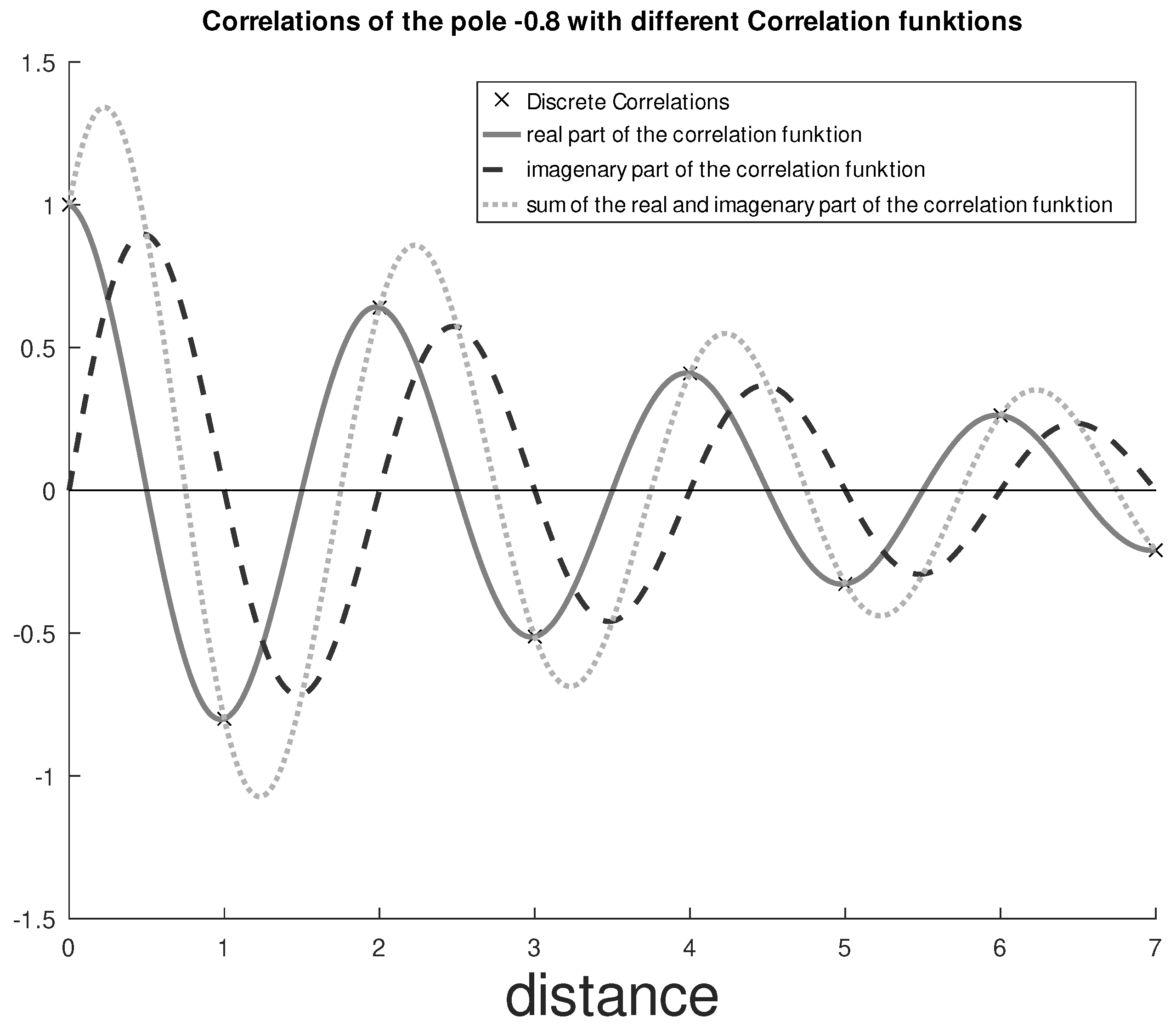
2.1. Construction of a Continuous Covariance Function

The process S t is called one-dimensional AR process of order p (AR(p) process) if it is described by the recursive equation
S t = α 1 S t 1 + α 2 S t 2 + + α p S t p + E t
where α 1 , α 2 , ..., α p are the coefficients of the AR process and E t is a i.i.d. sequence with variance σ E 2 [17] (p. 58, Equation (3.4.31)). We assume that α p 0 , as otherwise the AR(p) process is also an AR ( p 1 ) process so that AR(p) is not well-defined (In addition, if α p = 0 some formulas in this paper cannot be used).
An important quantity is the zeros ( ζ l ) of an AR(p) process defined by the zeros of the characteristic polynomial
χ ( x ) = 1 α 1 x 1 α 2 x 2 α p x p = ( x ζ 1 ) ( x ζ 2 ) ( x ζ p ) ,
see e.g., [17] (p. 58, Equation (3.4.32)).
An alternative definition is given by the auxiliary equation if we interpret the AR process as a difference equation which has the general solution (see [19], p. 134, Equation (3.33))
b ( x ) = x p α 1 x p 1 α 2 x p 2 α p = ( x p 1 ) ( x p 2 ) ( x p p ) .
These zeros p l only occur as real values or in pairs of complex conjugated zeros. Bear in mind that the zeros of the characteristic polynomial from Equation (2) are linked to the zeros of the auxiliary equation (cf. Equation (3)) by ζ l = 1 / p l . AR processes are stationary if and only if the ζ l are outside the unit circle, such that | p l | < 1 . In the following we will restrict to p l for simplicity.
With this definitions in mind, the discrete covariances Σ j of an AR(p) process, are linked with each other by the Yule–Walker (YW) equations (see e.g., [17], p. 59, Equation (3.4.36)), i.e.,
Σ 0 = α 1 Σ 1 + α 2 Σ 2 + + α p Σ p + σ E 2
Σ j = α 1 Σ | j 1 | + α 2 Σ | j 2 | + + α p Σ | j p | if j 0 .
The YW equation of higher order than 0 (Equation (5)) are basically homogeneous difference equations of order p,
Σ j α 1 Σ | j 1 | α 2 Σ | j 2 | α p Σ | j p | = 0 .
The general solution to the difference equation can be expressed by the powers of the zeros p l of the auxiliary Equation (3). The particular solution is fixed by the boundary conditions using the discrete covariances determined from the YW equations (cf. Equation (5)),
Σ j = l = 1 p A l p l | j | .
Here A l are coefficients which are complex if and only if the corresponding p l is complex. Furthermore, if there is a pair of complex conjugated p l then A l occur also as complex conjugated pairs (see e.g., [18], p. 134, Equation (3.5.44) or [19], p.163, f.).
At this point a new but now continuous function is defined, which can be seen as the continuous covariance function γ ( h ) : R R for any AR(p) process,
γ ( h ) : = l = 1 p A l p l | h | .
Here A l and p l are the same as in Equation (7), but the domain changed. j N 0 is replaced by h R .
Attentive readers will have noticed that γ ( h ) is complex if any p l R . Then γ ( h ) C for all h N 0 . One important convention that will help with this inconsistency is the use of the real part Re γ ( h ) of the complex function (see Figure 1). This condition will not have any impact if γ ( h ) is real (what is mostly the case), and furthermore a covariance function for real valued signals is defined to be a function in R not in C .

2.2. Properties of the Continuous Covariance Function

Since with γ ( h ) from Equation (8) a suitable function is found to fit through the discrete covariances from Equation (7), we want to analyze the power spectral densities of the continuous and the discrete functions. On this basis we can demonstrate that the Fourier transform of the continuous covariance function is positive semi-definite.
Initially the problem restricted to AR processes of order 1 and order 2 with two complex conjugated zeros. On the one hand any AR(p) process can be dissected into a product of AR(1) and AR(2) processes. This is a linear function, so the power spectral function is the product of the corresponding AR(1) processes and AR(2) processes. On the other hand, Equation (8) shows that the covariance function is a weighted sum of the real valued zeros, or pairs of complex conjugated zeros. So, the zeros are also in a linear relation, and so is the Fourier transform. So, it is only necessary to examine the spectrum and the Fourier transform for the first order AR process and second order AR process with two complex conjugated zeros.
For these specific types of AR processes there is an analytical solution to switch from AR coefficients α l to the zeros p l (see [20]),
for order p = 1 α 1 = p 1
and for order p = 2 α 1 = p 1 + p 2 α 2 = p 1 p 2 with p 1 = p 2 .

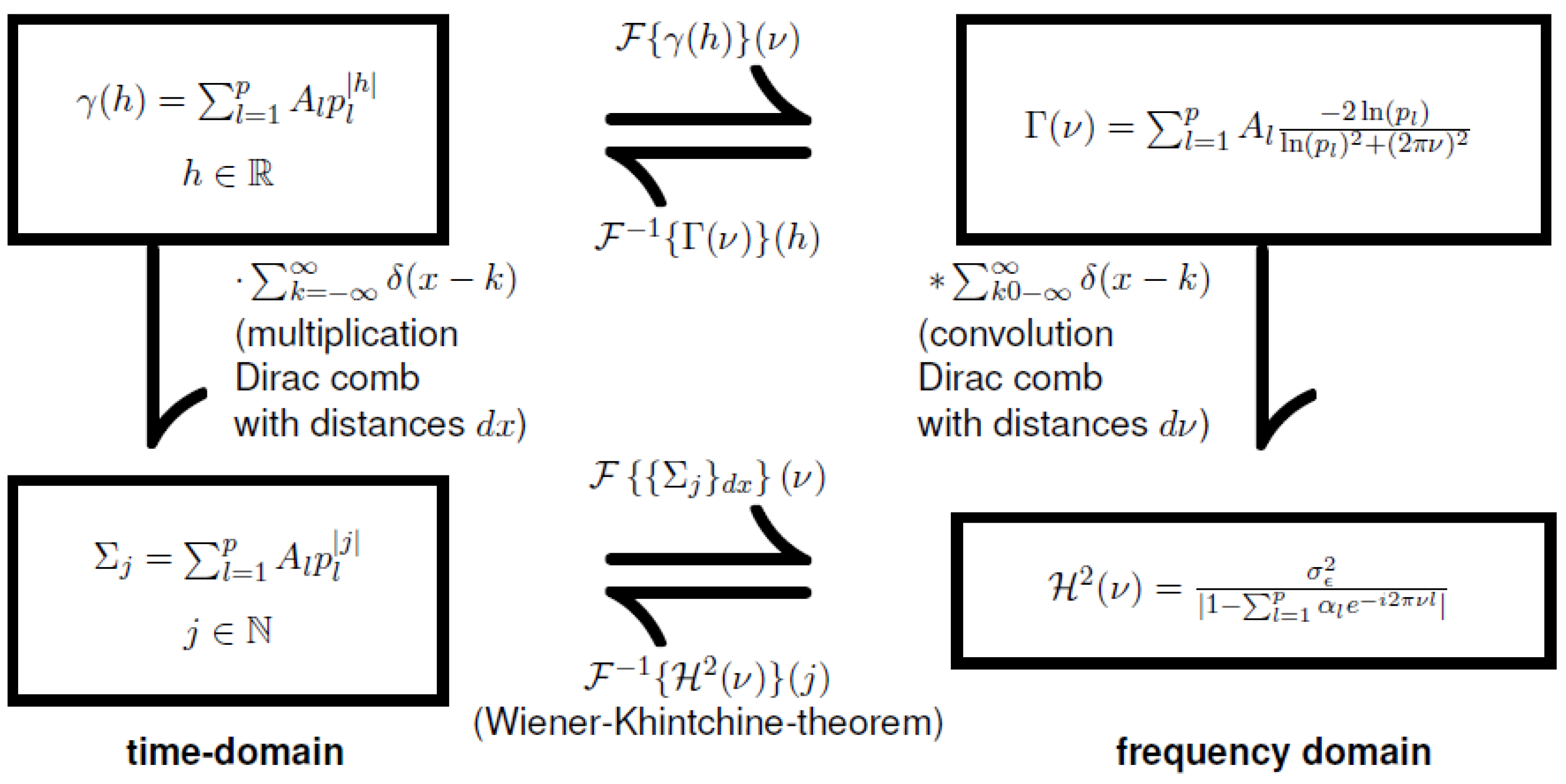
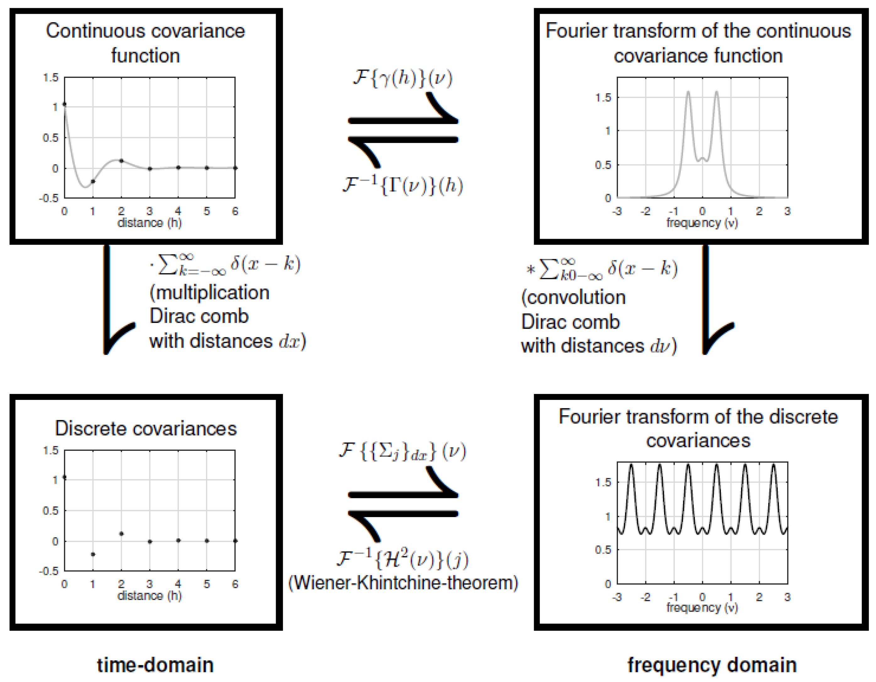
2.2.1. Power Spectral Density

The power spectral density for an AR(p) process is well known (see e.g., [16], p. 244, Equation (11.20)) and is described by the transfer function
H 2 ( ν ) = σ E 2 | 1 l = 1 p α l e i 2 π ν l | 2 .
In consideration of Equations (9) and (10) the power spectral density for any AR(1) process and AR(2) process with complex conjugated zero can be calculated explicitly. So, the power spectral density AR(1) process is generated via
H 2 ( ν ) = σ E 2 1 2 p 1 cos ( 2 π ν ) + p 1 2 .
For the AR(2) process with zeros p 1 = p 2 the power spectral density is a little more complicated and turns out to be
H 2 ( ν ) = σ E 2 1 2 ( p 1 + p 2 ) cos ( 2 π ν ) + p 1 p 2 2 + 2 cos ( 4 π ν ) ( p 1 + p 2 ) cos ( 2 π ν ) + p 1 p 2 + p 1 2 + p 2 2 .
Using the Fourier transform of the covariance function γ ( h )
Γ ( ν ) : = F { γ ( h ) } ( ν ) = l = 1 p A l 2 ln ( p l ) ln ( p l ) 2 + 2 π ν 2
is an alternative way to derive the power spectral density (For further derivations of the Fourier transform see Appendix A). However, H 2 ( ν ) Γ ( ν ) . Especially Equation (11) shows H 2 ( ν ) as a function whose only parameter ν arise as power of the complex function e i 2 π l . Therefore H 2 ( ν ) is a repetitive function with period 1. In contrast, Equation (14) shows Γ ( ν ) is aperiodic function with lim ν Γ ( ν ) = 0 . To understand this circumstance two theorems are of importance:
  • The discrete covariances of an AR(p) process ( Σ j ) are equivalent to the product of the Dirac comb with the continuous covariance function γ ( h ) .
  • The convolution theorem shows that multiplication in time domain results in convolution in frequency domain.
Combining these two pieces of information shows indeed that H 2 ( ν ) Γ ( ν ) but
H 2 ( ν ) = Γ ( ν ) k = δ ( x k )
where k = δ ( x k ) is the Dirac comb of distance 1 and Γ ( ν ) k = δ ( x k ) is the convolution of Γ ( ν ) and the Dirac comb. The transitions from continuous functions to discrete sequences as well as the resulting Fourier transforms are shown in Figure 2 (For a more detailed method of calculation for AR(1) and AR(2) processes see Appendix C).

2.2.2. Positive Semi-Definite Function

Equation (15) shows that knowing if H 2 ( ν ) is positive semi-definite is not sufficient to guarantee that the Fourier transform of the continuous function γ ( h ) is positive semi-definite too. Therefore, the explicit Fourier transforms of the AR(1) and AR(2) process are derived here. For the case of the AR(1) process it is easy to see that for the Fourier transform of the covariance function γ ( h )
Γ ( ν ) = σ E 2 1 p 2 2 ln ( p ) ln ( p ) 2 + 2 π ν 2 > 0 ν R .
holds (For the derivation of this formula see Appendix B.1). Neither the squared terms could be less than 0 nor 1 p 2 or ln ( p ) due to the fact that p lies within the unit circle.
For the AR(2) process things are not that obvious. In Appendix B.2 it is demonstrated that the Fourier transform of γ ( h ) is
Γ ( ν ) = 2 Re σ E 2 p 1 ( p 2 p 1 ) ( 1 p 1 2 ) ( 1 p 1 p 2 ) 2 ln ( p 1 ) ( ln ( p 1 ) ) 2 + ( 2 π ν ) 2 .
To work with complex valued fractions, it is necessary to eliminate the imaginary part in the denominator. This is done by multiplying each term of the sum with the complex conjugated denominator divided by itself. Afterwards it is simple to pick the real part. To simplify the formula, we use the polar coordinates p 1 = r e i ϕ , and p 2 = r e i ϕ with 0 < r < 1 and 0 ϕ π . So, it can be shown that the numerator is positive ( Γ ( ν ) 0 ) if and only if
ln ( r ) coth ( ln ( r ) ) : = f ( r ) ϕ cot ( ϕ ) : = g ( ϕ )
The function f ( r ) and g ( ϕ ) are displayed in Figure 3 and Figure 4 (Since g ( ϕ ) = g ( ϕ ) , the negative values of ϕ are not needed). On the one hand f ( r ) is a declining function with infimum 1. On the other hand, the function g ( ϕ ) is also declining, with a maximum of 1. Thus, infimum f ( r ) max g ( ϕ ) , which evaluate that Equation (18) is always satisfied.

3. Simulation

To visualize the results from Section 2 of an AR(3) process with two complex conjugated zeros was generated as an example. First to guarantee stationarity the roots are chosen as
p 1 p 2 p 3 = 0.252 0.126 i 0.252 + 0.126 i 0.306 .
Let the variance of the white noise be σ ϵ 2 = 1. After deriving the coefficients α l , l { 1 , 2 , 3 } , using Equation (3), we estimate the discrete covariances ( Σ j ) of the AR(3) process by the reorganized YW equations (see [21], p. 32, Equation (183)). With Equation (8) a continuous function γ ( h ) is fitted through the discrete covariances (see the left upper corner of Figure 5). Subsequently the power spectral density is set first by Equation (11) using the coefficients α l and secondly by Equation (14). For the second step the coefficients A l are estimated by solving the system of equations
Σ 0 Σ 1 Σ 2 = 1 1 1 p 1 p 2 p 3 p 1 2 p 2 2 p 3 2 A 1 A 2 A 3 .
Here the zeros p l and covariances Σ l are known. Each row represents Equation (7) for l { 1 , 2 , 3 } . The coefficients A l are used in Equation (8) to estimate the power spectral density of the continuous covariance function. It must be mentioned that this example is an extreme one where the Fourier transform of the continuous covariance function has high values for frequencies higher the Nyquist frequency ν n = 0.5 . The Fourier transform of the continuous covariance function is not periodic at all (compare right upper corner of Figure 5). However, periodicity is the characteristic of the spectral density of a discrete AR process. Therefore, the periodicity is a result of the convolution of the Dirac comb and Γ ( ν ) .

4. Conclusions and Outlook

In this paper, it was shown that the choice of a valid continuous covariance function for AR(p) processes is given by the function
γ ( h ) = l = 1 p A l p l | h | .
Here h R is the lag, p l are the roots of the characteristic polynomial, and A l follows from the unique solution of Equation (14) for p arbitrarily chosen discrete covariances Σ j 1 , Σ j 2 , ..., Σ j p (with j i N 0 , and j i j k i k ):
A 1 A 2 A p = p 1 j 1 p 2 j 1 p p j 1 p 1 j 2 p 2 j 2 p p j 2 p 1 j p p 2 j p p p j p 1 Σ j 1 Σ j 2 Σ j p .
Due to the convolution theorem, the power spectral density of γ ( h ) might be different to the power spectral density of the discrete AR(p) process. Nevertheless, the proof was given that γ ( h ) is still positive semi-definite (cf. Section 2.2.2), and consequently meets all conditions for a suitable covariance function. The Fourier transforms Γ ( ν ) and H 2 ( ν ) may not vary much for ν [ 1 , 1 ] and the simulation (see Section 3) is an extreme example. Anyway γ ( h ) is an exponential function, so it is easy to use it as functional for covariance function propagation or LSC.
In further works the continuous covariance function γ ( h ) could be extended to a function for an autoregressive moving average (ARMA) process to examine its properties. It is not yet demonstrated that the oscillation of Re ( γ ( h ) ) leads towards the minimal frequency if there is a real negative zero ( p l = 0 for any l).

Author Contributions

Conceptualization, methodology, formal analysis, investigation, software, validation, visualization, data curation, writing—Original draft preparation: J.K., writing—Review and editing: J.K., T.S., J.M.B. and W.-D.S., funding acquisition, project administration, resources, supervision: W.-D.S. All authors have read and agreed to the published version of the manuscript.

Funding

This research is funded by the Deutsche Forschungsgemeinschaft (DFG, German Research Foundation)—Grant No. 435703911 (SCHU 2305/7-1 ‘Nonstationary stochastic processes in least squares collocation—NonStopLSC’).

Conflicts of Interest

The authors declare no conflict of interest.

Appendix A. General Fourier Transform of an AR(p) Process

In this part the Fourier transform of a function γ ( h ) = l = 1 p A l p l | h | with h R is computed,
Γ ( ν ) = l = 1 p A l p l | h | e i 2 π ν h d h = l = 1 p A l 0 p l h e i 2 π ν h d h 1 ln ( p l ) i 2 π ν + 0 p l h e i 2 π ν h d h 1 ln ( p ) + i 2 π ν = l = 1 p A l 2 ln ( p l ) ( ln ( p l ) ) 2 + ( 2 π ν ) 2
Please note that A l and p l might be complex, but this will not have any influence on the equations.

Appendix B. Explicit Fourier Transform of the AR(1) Process and AR(2) Process with Two Complex Conjugated Zeros

In this section, the explicit Fourier transform Γ ( ν ) of the continuous covariance function γ ( h ) for the orders p = 1 and p = 2 are given as function of h, and the zeros p l .

Appendix B.1. Fourier Transform of the Continuous Covariance Function of AR(1) Processes

First the discrete covariance Σ 0 must be computed as function of the zero p 1 . This is done by the reorganized YW equations (see [21], p. 32, Equation (183)):
1 0 α 1 1 + 0 α 1 0 0 1 σ ϵ 2 0 = Σ 0 Σ 1 1 1 α 1 2 1 α 1 α 1 1 σ ϵ 2 0 = Σ 0 Σ 1
Σ 0 = σ ϵ 2 1 α 1 2
Further Equation (7) gives Σ 0 = A 1 and in combination with Equation (9) the deduction is
A 1 = σ ϵ 2 1 p 1 2 .
Insert A 1 in Equation (14) for order p = 1 to obtain
Γ ( ν ) = σ ϵ 2 1 p 1 2 2 ln ( p 1 ) ln ( p 1 ) 2 + 2 π ν 2 .

Appendix B.2. Fourier Transform of the Continuous Covariance Function of AR(2) Processes with Two Complex Conjugated Zeros

Like in the last subsection the discrete covariances Σ 0 and Σ 1 are computed by the reorganized YW equations:
1 0 0 α 1 1 0 α 2 α 1 1 + 0 α 1 α 2 0 α 2 0 0 0 0 1 σ ϵ 2 0 0 = Σ 0 Σ 1 Σ 2 σ ϵ 2 α 2 2 + α 2 2 + α 2 ( 1 + α 1 2 ) + α 1 2 1 1 α 2 α 1 α 1 2 α 2 2 + α 2 = Σ 0 Σ 1 Σ 2 .
With the transformation from α 1 , α 2 to p 1 , p 2 (cf. Equation (10)) the discrete covariances are set by
Σ 0 = ( 1 + p 1 p 2 ) σ ϵ 2 ( p 1 2 1 ) ( 1 p 2 2 ) ( 1 p 1 p 2 ) Σ 1 = ( p 1 + p 2 ) σ ϵ 2 ( p 1 2 1 ) ( 1 p 2 2 ) ( 1 p 1 p 2 ) .
This time Equation (7) is an equation system in the two variables A 1 and A 2 . Here the first and second discrete covariances ( Σ 0 , Σ 1 ) are used:
Σ 0 Σ 1 = 1 1 p 1 p 2 A 1 A 2 A 1 A 2 = 1 1 p 1 p 2 1 Σ 0 Σ 1 A 1 A 2 = 1 p 2 p 1 p 2 1 p 1 1 Σ 0 Σ 1
A 1 = p 2 Σ 0 Σ 1 p 2 p 1 ; A 2 = p 1 Σ 0 Σ 1 p 1 p 2
Including the solution for Σ 0 and Σ 1 to obtain A 1 and A 2 as function of p 1 and p 2 leads to
A 1 = p 1 σ ϵ 2 ( p 2 p 1 ) ( 1 p 1 2 ) ( 1 p 1 p 2 ) ; A 2 = p 2 σ ϵ 2 ( p 1 p 2 ) ( 1 p 2 2 ) ( 1 p 1 p 2 )
Due two p 1 = p 2 , inserting A 1 and A 2 in Equation (14) leads to the sum of two complex conjugated values. This is equally to two times the real part of the complex value:
Γ ( ν ) = A 1 2 ln ( p 1 ) ln ( p 1 ) 2 + 2 π ν 2 + A 2 2 ln ( p 2 ) ln ( p 2 ) 2 + 2 π ν 2 = 2 Re A 1 2 ln ( p 1 ) ln ( p 1 ) 2 + 2 π ν 2 = 2 Re σ E 2 p 1 ( p 2 p 1 ) ( 1 p 1 2 ) ( 1 p 1 p 2 ) 2 ln ( p 1 ) ( ln ( p 1 ) ) 2 + ( 2 π ν ) 2

Appendix C. Convolution of the Fourier Transform of a Continuous Covariance Function of an AR Process with a Dirac Comb

The convolution theorem means if F ( ν ) and G ( ν ) are the Fourier transforms of the function f ( h ) and g ( h ) , then
F { f ( h ) g ( h ) } ( ν ) = F ( ν ) G ( ν ) .
In this context, f ( x ) = γ ( h ) (see Equation (8)) and F ( ν ) = Γ ( ν ) (see Equation (14)). For g ( x ) = k = δ ( x k ) (the Dirac comb of distance d x = 1 ) the Fourier transform is again a Dirac comb of distance d ν = 1 / d x = 1 . So, in the time domain is the same function as in the frequency domain (for ν = x : G ( ν ) = g ( x ) ). Using these results leads to
F γ ( h ) k = δ ( x k ) ( ν ) = Γ ( ν ) k = δ ( ν k ) = Γ ( u ) k = δ ( u ν k ) d u = ( i ) k = Γ ( u ) δ ( u ( ν + k ) ) d u = ( i i ) k = Γ ( ν + k ) = ( i i i ) k = γ ( h ) e i 2 π ν h e i 2 π k h d h = l = 1 p A l k = p l | h | e i 2 π ν h e i 2 π k h d h .
In step (i) the sum and the integral are exchanged. Step (ii) represents the ability of the Dirac impulse that f ( u ) δ ( u x ) d u = f ( x ) . Finally, (iii) uses the frequency shift of the inverse Fourier transform (see e.g., [16], p. 26, Table 2.2). Using this function to compute the power spectral density for an AR(1) process will result in Equation (12) or in the case of an AR(2) process with two complex conjugated zeros in Equation (13).

References

  1. Förstner, W. Determination of the additive noise variance in observed autoregressive processes using variance component estimation technique. Stat. Decis. 1985, 2, 263–274. [Google Scholar]
  2. Förstner, W.; Wrobel, B.P. Photogrammetric Computer Vision–Statistics; Springer: Berlin/Heidelberg, Germany, 2016; Volume 6. [Google Scholar]
  3. Koch, K. Rekursive Numerische Filter. Z. Für Vermess. 1975, 100, 281–292. [Google Scholar]
  4. Schuh, W.D. Tailored Numerical Solution Strategies for the Global Determination of the Earth’s Gravity Field; Mitteilungen Der Geodätischen Institute, Technische Universität Graz (TUG): Graz, Austria, 1996; Volume 81. [Google Scholar]
  5. Zeng, W.; Fang, X.; Lin, Y.; Huang, X.; Zhou, Y. On the total least-squares estimation for autoregressive model. Taylor Fr. 2018, 50, 186–190. [Google Scholar] [CrossRef]
  6. Krarup, T. A Contribution to the Mathematical Foundation of Physical Geodesy; Number 44 in Meddelelse; Danish Geodetic Institute: Copenhagen, Denmark, 1969. [Google Scholar]
  7. Moritz, H. Advanced Least-Squares Methods; Number 175 in Reports of the Department of Geodetic Science, Ohio State University Research Foundation: Columbus, OH, USA, 1972. [Google Scholar]
  8. Moritz, H. Least-Squares Collocation; Number 75 in Reihe A; Deutsche Geodätische Kommission: München, Germany, 1973. [Google Scholar]
  9. Dermanis, A. Kriging and collocation: A comparison. Manuscr. Geod. 1984, 9, 159–167. [Google Scholar]
  10. Schuh, W.D. Signalverarbeitung in Der Physikalischen Geodäsie. In Handbuch Der Geodäsie, Erdmessung Und Satellitengeodäsie; Freeden, W., Rummel, R., Eds.; Springer Reference Naturwissenschaften; Springer: Berlin/Heidelberg, Germany, 2016; pp. 73–121. [Google Scholar] [CrossRef]
  11. Schuh, W.D.; Brockmann, J. The Numerical Treatment of Covariance Stationary Processes in Least Squares Collocation. In Handbuch Der Geodäsie; Freeden, W., Ed.; Springer: Berlin/Heidelberg, Germany, 2018. [Google Scholar] [CrossRef]
  12. Moritz, H. Advanced Physical Geodesy; Wichmann: Karlsruhe, Germany, 1980. [Google Scholar]
  13. Reguzzoni, M.; Sansó, F.; Venuti, G. The Theory of General Kriging, with Applications to the Determination of a Local Geoid. Geophys. J. Int. 2005, 162, 303–314. [Google Scholar] [CrossRef] [Green Version]
  14. Box, G.E.P.; Jenkins, G.M.; Reinsel, G.C. Time Series Analysis: Forecasting and Control, Fourth Edition; Wiley Series in Probability and Statistics; John Wiley & Sons: Hoboken, NJ, USA, 2008. [Google Scholar] [CrossRef]
  15. Brockwell, P.J.; Davis, R.A. Time Series Theory and Methods, 2nd ed.; Springer Series in Statistics; Springer: New York, NY, USA, 1991. [Google Scholar] [CrossRef]
  16. Buttkus, B. Spectral Analysis and Filter Theory in Applied Geophysics; Springer: Berlin/Heidelberg, Germany, 2000. [Google Scholar] [CrossRef]
  17. Hamilton, J.D. Time Series Analysis; Princeton University Press: Princeton, NJ, USA, 1994. [Google Scholar]
  18. Priestley, M.B. Spectral Analysis and Time Series; Academic Press: London, UK; New York, NY, USA, 1981. [Google Scholar]
  19. Goldberg, S. Introduction to Difference Equations; Reprint ed.; Dover Publications: Mineola, NY, USA, 1986. [Google Scholar]
  20. Viète, F. Opera Mathematica, 1579; Reprinted in Leiden, Netherlands, 1646. [CrossRef]
  21. Schuh, W.D.; Krasbutter, I.; Kargoll, B. Korrelierte Messung—Was Nun. In Zeitabhängige Messgrößen—Ihre Daten Haben (Mehr-) Wert; Neuner, H., Ed.; DVW-Schriftenreihe; Wißner: Augsburg, Germany, 2014; Volume 74, pp. 85–101. [Google Scholar]
Figure 1. Real part, imaginary part and sum of both parts of a complex covariance function of an AR process with pole −0.8.
Engproc 05 00018 g001
Figure 2. Magic square for the convolution of a continuous covariance function with a Dirac comb.
Engproc 05 00018 g002
Figure 3. The function f ( r ) = ln ( r ) coth ( ln ( r ) ) for 0 < r < 1 .
Engproc 05 00018 g003
Figure 4. The function g ( ϕ ) = ϕ cot ( ϕ ) for 0 ϕ π , and an enlarged section of the beginning.
Engproc 05 00018 g004
Figure 5. Magic square for a convolution of a continuous covariance function of an AR(3) process with a Dirac comb.
Engproc 05 00018 g005
Publisher’s Note: MDPI stays neutral with regard to jurisdictional claims in published maps and institutional affiliations.

