
On the Family of Covariance Functions Based on ARMA Models †


Institute of Geodesy and Geoinformation, University of Bonn, 53115 Bonn, Germany
*
Author to whom correspondence should be addressed.
†
Presented at the 7th International conference on Time Series and Forecasting, Gran Canaria, Spain, 19–21 July 2021.
Eng. Proc. 2021, 5(1), 37; https://doi.org/10.3390/engproc2021005037
Published: 5 July 2021
(This article belongs to the Proceedings of The 7th International Conference on Time Series and Forecasting)
Abstract
:In time series analyses, covariance modeling is an essential part of stochastic methods such as prediction or filtering. For practical use, general families of covariance functions with large flexibilities are necessary to model complex correlations structures such as negative correlations. Thus, families of covariance functions should be as versatile as possible by including a high variety of basis functions. Another drawback of some common covariance models is that they can be parameterized in a way such that they do not allow all parameters to vary. In this work, we elaborate on the affiliation of several established covariance functions such as exponential, Matérn-type, and damped oscillating functions to the general class of covariance functions defined by autoregressive moving average (ARMA) processes. Furthermore, we present advanced limit cases that also belong to this class and enable a higher variability of the shape parameters and, consequently, the representable covariance functions. For prediction tasks in applications with spatial data, the covariance function must be positive semi-definite in the respective domain. We provide conditions for the shape parameters that need to be fulfilled for positive semi-definiteness of the covariance function in higher input dimensions.
1. Introduction and Related Work
Signal covariance modeling is an important part of stochastic methods [1]. In covariance modeling, the choice of the type of covariance function is commonly separated from the actual estimation of its shape parameters. Thus, the estimated covariance model quite strongly depends on the assessed basis functions. From this standpoint, it is desirable to have a very general class of covariance functions that can represent very different shapes with a single functional model and thus includes a large set of possible basis functions. A drop towards negative correlations, i.e., the so-called hole effect [2], is a widespread phenomenon in real-world datasets.
The Matérn family of covariance functions [3] finds application in many fields such as machine learning [4], environmental sciences, and geostatistics [5,6]. Simultaneously, a very similar class is known as Markov models, e.g., [6,7,8]. For instance, the combination of a degree-two polynomial and an exponential function is known as the third-order Markov model.
In geodetic time series analysis, many standard covariance models have been introduced early. For instance, the authors of [9] provided an application of a simple case of the Matérn covariance function to describe the stochastics of the gravity field. The authors of [10] and [11] introduced second- and third-order Markov models in the geodetic context; see also [12]. The author of [13] used the exponentially damped cosine in a geodetic application. Later, the second-order Markov model was applied to altimetry data [14,15].
On the other hand, Markov models are also referenced by different names. e.g., the respective models can be derived from Radon transforms of the exponential model, cf. [16] (p. 85). In the literature, these models are also denoted as second-order autoregressive (SOAR) models and third-order autoregressive (TOAR) models; see e.g., [8,17,18,19,20,21]. Despite the uncertain terminology in the literature, we distinguish between second-order Gauss–Markov (SOGM) models as in [22,23] and second-order Markov (SOM) models [7,8,10], whereas both models share the property of being second-order autoregressive (SOAR) or second-order ARMA models.
In [23], it was shown that the covariance function of AR and ARMA processes with unique poles corresponds to a sum of SOGM process covariance functions, which are a combination of an exponential function and cosine and sine terms. However, if the autoregressive poles are repeated, the correspondence to SOGM models does not hold anymore. Instead, a higher pole-multiplicity introduces polynomials as basis functions into the family of covariance functions. This more general family is commonly related back to [24] (p. 543) where a family of covariance functions constructed by polynomial functions and exponential damping terms is derived from ARMA models. Whilst the family is mostly introduced in the literature only for real poles, it has a complete set of covariance functions of oscillating type, which is discussed in this work. Examples of this general class appear very sparse in the literature, e.g., in [2] or in a short note on oscillatory Matérn covariance functions in [25] (Section 2.3.3) but never the complete variety of this class. In this work, we merge many known covariance functions to a combined family of covariance functions, namely the ARMA models.
Next to the variety of basis functions involved in the construction of a covariance function, it is essential for the function’s flexibility to allow all shape parameters to vary. By this requirement, one can define a family of covariance function, e.g., the class of Markov models. The reference with the most complete variety of functions belonging to this class is [5] (known as Buell’s function of index 3; see also [6]) who provides that model with enhanced variability of parameters, which is the general idea in this paper.
In this work, these two extensions to the standard covariance models are introduced as part of the family of non-repeated and repeated poles ARMA models. Hence, starting from the Matérn-type covariance models, it is intended to provide both a variety of basis functions and variability of the shape parameters to achieve the most general family of covariance functions.
Another aspect is the necessity of covariance functions being positive semi-definite. For applications with data in higher dimensions, e.g., spatial data, the reduction to a one-dimensional distance-like norm (e.g., Euclidean) does not guarantee positive definiteness of the covariance function in the higher dimension. Instead, the Bochner theorem extends to the Hankel transform being positive [1,26]. We derived the conditions among the shape parameters that ensure positive semi-definiteness of the covariance function in higher input dimensions.
2. The Family of Non-Repeated Poles ARMA Models
Reference [23] presents elegant parametrizations and fitting procedures for the family of covariance functions defined by autoregressive moving average (ARMA) models. The family is based on covariance functions defined by SOGM processes given in one of the two following parametrizations:
In more detail, the interpolating function to the discrete covariances of an AR(p) process is given by the following finite weighted sum of exponentiated (unique) autoregressive poles :
cf. [27] (Equation (5.2.44)) and [28] (Equation (3.5.44)), which can be mathematically converted to the representation of Equation (2); see [23]. Equation (3) corresponds to either a pure AR(p) process or an ARMA(p,q) process, depending on whether the weights are purely, i.e., uniquely, determined by the autoregressive poles . The two-step approach in [23] starts with an estimation of the autoregressive process parameter and concludes with the fitting of weighting coefficients of the interpolating function.
Positive Definiteness in Higher Dimensions
The application in spatial domains requires positive semi-definiteness of the covariance function in higher dimensions , which is derived here.
Starting from the simple exponentially damped cosine, e.g., [16] (p. 92), the SOGM covariance function is a generalization with three parameters, i.e., additional phase, see [23] for details on the parametrization. Similar to [29] (p. 26), positive semi-definiteness constraints on the parameters can be followed from [30] and amount to
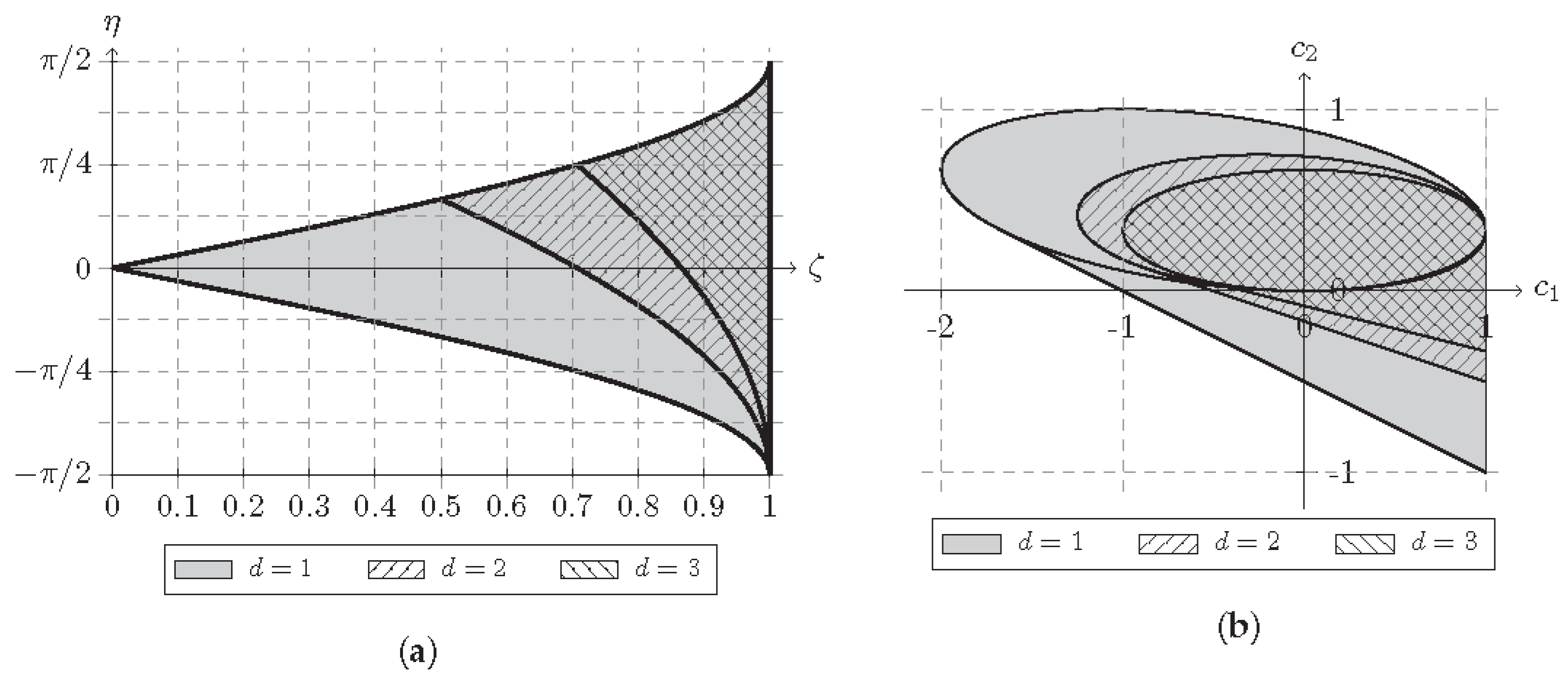
as an additional condition to the requirement , cf. [23]. The permissible area of parameters is illustrated in Figure 1a and is visibly restricted more and more with increasing dimension.
3. Generalization to Repeated Poles ARMA Models
Prior to providing the methodology of repeated poles ARMA processes, we introduce the basics of the Matérn family of covariance functions. The Matérn family of covariance functions can be parameterized in a way such that similarities to the ARMA models become clear.
3.1. The Half-Integer Matérn Covariance Function
The Matérn class of covariance Functions [3,4] defines a covariance functions with the two shape parameters c (scale of correlation length) and order . The Matérn covariance function is defined as
and, in the case of half-integers , simplifies to a combination of a polynomial of degree and an exponential function [4,6]. For the first four half-integers, we have
Note that the attenuation factor c also builds the coefficients of the polynomial.
3.2. Repeated Poles ARMA Models
Equation (3) holds only for the simple case assuming that the autoregressive process has distinct roots. When there are repeated real (positive or negative) poles or repeated complex conjugate poles, special cases have to be considered. Derived from the solution to the difference equation of the autoregressive relation for repeated poles, cf. e.g., [31] (Chap. 3.7), the required basis functions are summarized as one of the following cases of covariance sequences at discrete lags k, either
for , or
for the case , or finally
for . m represents the multiplicity of real roots, l represents the pairwise complex conjugate roots, and is the weights. As a result, these formulae correspond to multiplication and exponentiation of complex-valued weights and poles similar to Equation (3) and with the same correspondences , , and ; see [23] (Sections 4.3 and 5.1). However, for repeated poles, e.g., as visible from Equation (7), the summation is performed in the following way
Although the solution to the difference equation holds for discrete , we pursue a reinterpretation as a continuous covariance function ; see [23] (Section 4.3), and use the mathematical elegance of Equation (10) also for the analytical covariance function defined by AR or ARMA models.
From Equation (7), it is evident now that the Matérn covariance functions of order correspond to ARMA models with repeated real poles . As known, from the Matérn family, with increasing order , the squared-exponential (Gauss-type) covariance function is asymptotically reached. Hence, with increasing pole multiplicity, an increasingly lower slope at the origin is realized.
3.3. Bounds for the Polynomial Coefficients of Markov Models
For the purpose of increasing the flexibility, we adopt the half-integer Matérn covariance function but with arbitrary polynomial coefficients. This approach is followed in [5] with his function of index 3; see also [6]. Similar to [5], we intend to construct a general model with arbitrary weights
e.g., with third-order , which we denote as a third-order Markov (TOM) model.
As known from [23] (Section 5), allowing arbitrary weights between the basis functions creates a correspondence to ARMA models, i.e., introducing a moving average part. Hence, the covariance functions of index 3 of [5] as well as also have triple real poles, but they correspond to ARMA(3,q) processes with triple real poles but with unknown order of the moving average part here.
Note that, due to the fixed polynomial coefficients, the Matérn covariance functions determined by c are automatically positive definite for , which makes them simple and easy to handle. However, Markov models with adjustable coefficients exhibit greater flexibility, and they are viable for practical use if the bounds of the coefficients for positive (semi)-definiteness are known.
As in [6] (Equation (14)), we can construct the general model with arbitrary weights and from a combination of the half-integer Matérn models Equation (6). The correspondence is
In the d-dimensional space, the general Matérn covariance function has the Fourier transform
cf. [32] (Equation (4.130)), which, weighted as in Equation (12) and simplified (cf. [6]), yields
From this, bounds for the non-negativity conditions can be derived. In detail, can lie within the bounds defined by the functions
which form the shape of an ellipsis added to a straight line. If is larger than , the domain extends to the straight line lower bound / and up to and ; see Figure 1b.
3.4. Oscillatory Repeated Poles ARMA Models
It is intuitive to combine the Matérn covariance function with an oscillating function in order to create a more versatile function; see [25] (Section 2.3.3). Hence, by multiplying Equation (11) with a cosine of frequency a and phase , we have the following:
We define the general class of repeated poles ARMA covariance functions with times repeated complex-conjugate pairs of poles given by
and thus autoregressive order . Again, the moving average parameters, i.e., also the dependence of weights on poles and zeros of the ARMA process, are not derived here, cf. [23].
When combining the covariance models of Section 2 and Section 3.3, the conditions of positive definiteness are the joint requirements of both types, i.e., Figure 1a,b.
4. Application to Altimetry Data: A Demonstration
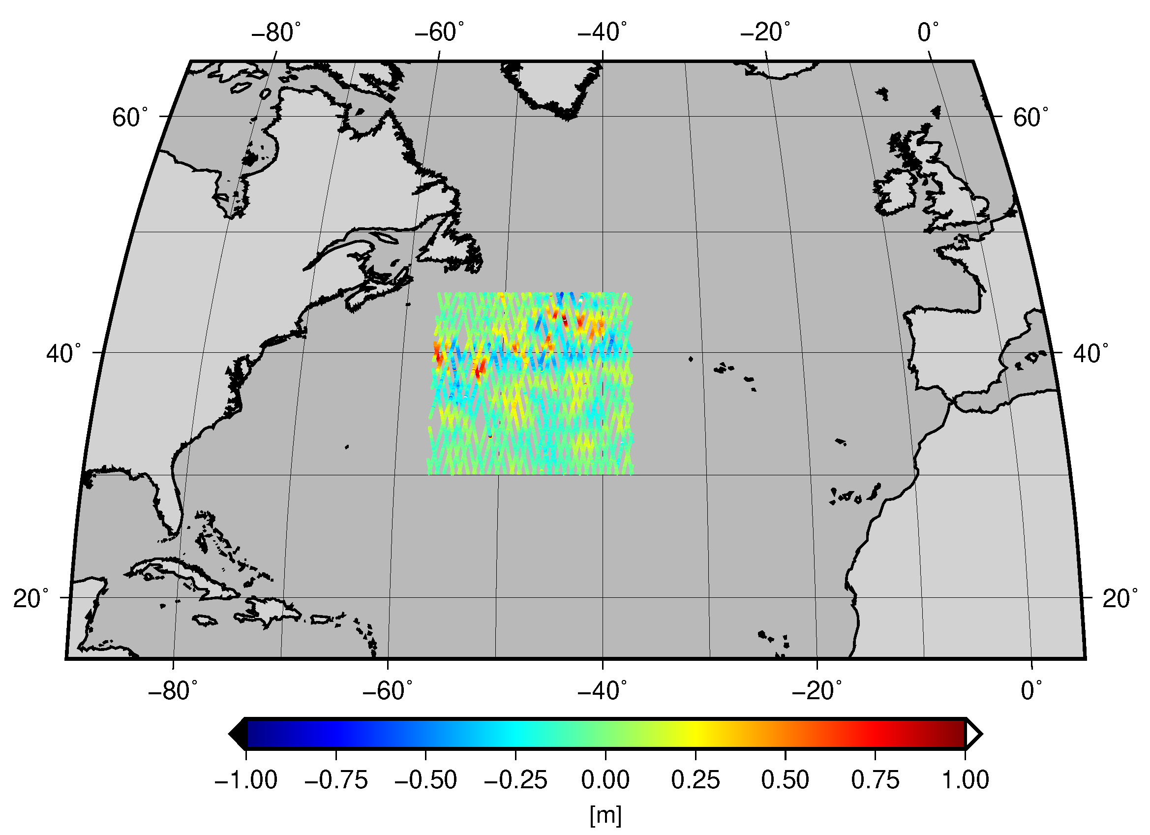
The following empirical covariance function of a two-dimensional geodetic application shall serve as a small example to demonstrate the necessity of different covariance functions presented in this work. Here, we interpret a time series of sea level anomalies (SLA) along the altimeter track as a stationary stochastic field in planar approximation, i.e., two-dimensional domain. To obtain SLA, sea surface heights observed by the Envisat satellite launched and operated from 2002 until 2012 by the European Space Agency were reduced by a long-term mean sea surface model (in this case, CNES-CLS11, [33]) interpolated along the satellites ground track. For the demonstration example, we extracted a subset of 10,905 observations in a local area of the North Atlantic ocean of cycle 13 (13 January 2003 to 17 February 2003); see Figure 2. We computed empirical estimates of the isotropic covariance function averaged for equidistant lags () and by using the biased estimator (see the black dots in Figure 3).
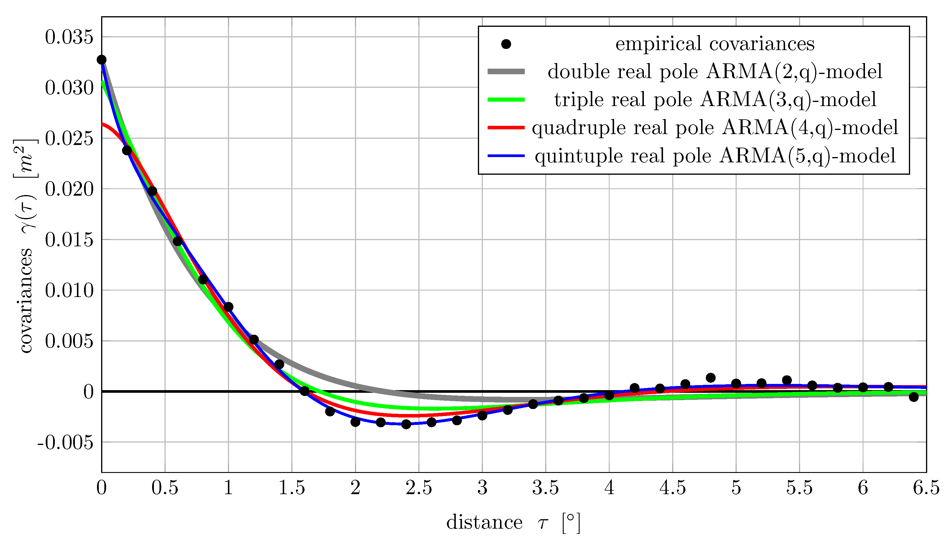
For Figure 4, we fit functions of the type in Equation (16) with different orders to the empirical covariances. These ARMA models do not experience an improvement from the higher pole multiplicity because the oscillatory nature of the complex poles ARMA model already nicely captures the hole effect. The higher-order models slightly improve the very long-range correlations.
For demonstration purposes, different types of covariance functions belonging to the family of (repeated pole) ARMA models are fitted to the empirical estimates of the covariances from lag up to using non-closed-form solvers. We used the GNU Octave’s nonlinear minimization routine fmincon, cf. [34] and implemented a constrained least squares fitting.
In a first plot, we fit repeated real pole ARMA models, i.e., Equation (11), of orders and 5. These correspond to linear combinations of Matérn covariance functions, where some Matérn functions can even be subtracted in the combination. The number of fitted parameters, i.e., , c, and , are 3, 4, 5, and 6. The order q of the moving average part is not determined here. All results are estimated to be positive semi-definite in .
Figure 3 shows that the polynomial component of the covariance function can successfully capture the negative correlations. The quality of fit gets better with increasing order and is sufficient for the fifth-order model. We are aware that the nugget (white noise variance component) is quite different for the estimated models, but that is because we did not restrict it by a priori knowledge.
5. Summary and Conclusions
The example demonstrates that relatively complex correlations structures can also be captured by simple covariance models such as Markov models. Enhanced flexibility is achieved by adjustable polynomial coefficients, which makes them favorable to the Matérn covariance function, especially for modeling negative correlations as in the example. The underlying methodology of ARMA processes builds the general family for all of these covariance functions and thus also holds out the prospect of suited optimization methods such as the Yule–Walker equations, cf. [23].
In addition, we provide bounds for all parameters of the ARMA covariance models in order to ensure positive semi-definiteness in the respective domain of the data. In general, this work demonstrates the necessity for a large variety of basis functions collected in a family of covariance functions as well as suited fitting procedures. Tailored optimization problems for the repeated poles ARMA models are still an open research field.
Author Contributions
Conceptualization, methodology, formal analysis, investigation, software, validation, visualization, writing—original draft preparation: T.S., writing—review and editing: T.S., J.K., J.M.B., and W.-D.S., data curation: J.M.B., funding acquisition, project administration, resources, supervision: W.-D.S. All authors have read and agreed to the published version of the manuscript.
Funding
This research is funded by the Deutsche Forschungsgemeinschaft (DFG, German Research Foundation) grant No. 435703911 (SCHU 2305/7-1 ‘Nonstationary stochastic processes in least squares collocation—NonStopLSC’). The second author acknowledges the financial support of the DFG in the context of the PARASURV (grant BR5470/1-1) project.
Data Availability Statement
The used Delayed Time CorSSH products were processed with support from CNES (by CLS Space Oceanography Division) and distributed by AVISO+ (http://www.aviso.altimetry.fr/, accessed on 2 October 2019).
Conflicts of Interest
The authors declare no conflict of interest.
Abbreviations
The following abbreviations are used in this manuscript:
| AR | Autoregressive |
| ARMA | Autoregressive moving average |
| MA | Moving average |
| SOGM | Second-order Gauss–Markov |
| SLA | Sea level anomalies |
References
- Moritz, H. Covariance Functions in Least-Squares Collocation; Number 240 in Reports of the Department of Geodetic Science; Ohio State University: Columbus, OH, USA, 1976. [Google Scholar]
- Journel, A.G.; Froidevaux, R. Anisotropic Hole-Effect Modeling. J. Int. Assoc. Math. Geol. 1982, 14, 217–239. [Google Scholar] [CrossRef]
- Matérn, B. Spatial Variation: Stochastic Models and Their Application to Some Problems in Forest Surveys and Other Sampling Investigations. Ph.D. Thesis, University of Stockholm, Stockholm, Sweden, 1960. [Google Scholar] [CrossRef]
- Rasmussen, C.; Williams, C. Gaussian Processes for Machine Learning; Adaptive Computation and Machine Learning; MIT Press: Cambridge, MA, USA, 2006. [Google Scholar]
- Buell, C.E. Correlation Functions for Wind and Geopotential on Isobaric Surfaces. J. Appl. Meteorol. 1972, 11, 51–59. [Google Scholar] [CrossRef]
- Gneiting, T. Correlation Functions for Atmospheric Data Analysis. Q. J. R. Meteorol. Soc. 1999, 125, 2449–2464. [Google Scholar] [CrossRef]
- Gelb, A. Applied Optimal Estimation; The MIT Press: Cambridge, MA, USA, 1974. [Google Scholar]
- Moreaux, G. Compactly Supported Radial Covariance Functions. J. Geod. 2008, 82, 431–443. [Google Scholar] [CrossRef]
- Shaw, L.; Paul, I.; Henrikson, P. Statistical Models for the Vertical Deflection from Gravity-Anomaly Models. J. Geophys. Res. (1896–1977) 1969, 74, 4259–4265. [Google Scholar] [CrossRef]
- Kasper, J.F. A Second-Order Markov Gravity Anomaly Model. J. Geophys. Res. (1896–1977) 1971, 76, 7844–7849. [Google Scholar] [CrossRef]
- Jordan, S.K. Self-Consistent Statistical Models for the Gravity Anomaly, Vertical Deflections, and Undulation of the Geoid. J. Geophys. Res. (1896–1977) 1972, 77, 3660–3670. [Google Scholar] [CrossRef]
- Moritz, H. Least-Squares Collocation. Rev. Geophys. 1978, 16, 421–430. [Google Scholar] [CrossRef]
- Vyskočil, V. On the Covariance and Structure Functions of the Anomalous Gravity Field. Stud. Geophys. Geod. 1970, 14, 174–177. [Google Scholar] [CrossRef]
- Andersen, O.B.; Knudsen, P. Global Marine Gravity Field from the ERS-1 and Geosat Geodetic Mission Altimetry. J. Geophys. Res. Ocean. 1998, 103, 8129–8137. [Google Scholar] [CrossRef]
- Andersen, O.B. Marine Gravity and Geoid from Satellite Altimetry. In Geoid Determination: Theory and Methods; Sansò, F., Sideris, M.G., Eds.; Lecture Notes in Earth System Sciences; Springer: Berlin/Heidelberg, Germany, 2013; pp. 401–451. [Google Scholar] [CrossRef]
- Chilès, J.P.; Delfiner, P. Geostatistics: Modeling Spatial Uncertainty; Wiley Series in Probability and Statistics; John Wiley & Sons: Hoboken, NJ, USA, 1999. [Google Scholar] [CrossRef]
- Julian, P.R.; Thiébaux, H.J. On Some Properties of Correlation Functions Used in Optimum Interpolation Schemes. Mon. Weather. Rev. 1975, 103, 605–616. [Google Scholar] [CrossRef]
- Thiébaux, H.J. Anisotropic Correlation Functions for Objective Analysis. Mon. Weather. Rev. 1976, 104, 994–1002. [Google Scholar] [CrossRef] [Green Version]
- Franke, R.H. Covariance Functions for Statistical Interpolation; Technical Report NPS-53-86-007; Naval Postgraduate School: Monterey, CA, USA, 1986. [Google Scholar]
- Weber, R.O.; Talkner, P. Some Remarks on Spatial Correlation Function Models. Mon. Weather. Rev. 1993, 121, 2611–2617. [Google Scholar] [CrossRef]
- Gaspari, G.; Cohn, S.E. Construction of Correlation Functions in Two and Three Dimensions. Q. J. R. Meteorol. Soc. 1999, 125, 723–757. [Google Scholar] [CrossRef]
- Maybeck, P.S. Stochastic Models, Estimation, and Control; Mathematics in Science and Engineering; Academic Press: New York, NY, USA, 1979; Volume 141-1. [Google Scholar] [CrossRef]
- Schubert, T.; Korte, J.; Brockmann, J.M.; Schuh, W.D. A Generic Approach to Covariance Function Estimation Using ARMA-Models. Mathematics 2020, 8, 591. [Google Scholar] [CrossRef] [Green Version]
- Doob, J.L. Stochastic Processes; Wiley Series in Probability and Mathematical Statistics; Wiley: New York, NY, USA, 1953. [Google Scholar]
- Li, Z. Methods for Irregularly Sampled Continuous Time Processes. Ph.D. Thesis, University College London, London, UK, 2014. [Google Scholar]
- Wackernagel, H. Multivariate Geostatistics: An Introduction with Applications; Springer: Berlin/Heidelberg, Germany, 1995. [Google Scholar] [CrossRef]
- Jenkins, G.M.; Watts, D.G. Spectral Analysis and Its Applications; Holden-Day: San Francisco, CA, USA, 1968. [Google Scholar]
- Priestley, M.B. Spectral Analysis and Time Series; Academic Press: London, UK; New York, NY, USA, 1981. [Google Scholar]
- Gelfand, A.E.; Diggle, P.; Guttorp, P.; Fuentes, M. Handbook of Spatial Statistics; Handbooks of Modern Statistical Methods; Chapman & Hall/CRC: Boca Raton, FL, USA, 2010. [Google Scholar] [CrossRef]
- Zastavnyi, V.P. Positive Definiteness of a Family of Functions. Math. Notes 2017, 101, 250–259. [Google Scholar] [CrossRef]
- Goldberg, S. Introduction to Difference Equations; Dover Publications: New York, NY, USA, 1986. [Google Scholar]
- Yaglom, A.M. Correlation Theory of Stationary and Related Random Functions: Volume I: Basic Results; Springer Series in Statistics; Springer: New York, NY, USA, 1987. [Google Scholar]
- Schaeffer, P.; Faugére, Y.; Legeais, J.F.; Ollivier, A.; Guinle, T.; Picot, N. The CNES_CLS11 Global Mean Sea Surface Computed from 16 Years of Satellite Altimeter Data. Mar. Geod. 2012, 35, 3–19. [Google Scholar] [CrossRef]
- Eaton, J.W.; Bateman, D.; Hauberg, S.; Wehbring, R. GNU Octave; Version 5.2.0 Manual: A High-Level Interactive Language for Numerical Computations; Free Software Foundation: Boston, MA, USA, 2020. [Google Scholar]
Figure 1.
Permissible areas for parameters. For each dimension, the permissible area becomes a subset of that of the lower dimension. (a) Permissible areas of the parameters ζ and η in different dimensions 1 to 3. (b) Permissible areas of the weights c1 and c2 in different dimensions 1 to 3 shown for fixed parameter c = 1.

Figure 2.
Subset of the SLA data used for the example.

Figure 3.
Functions of the type in Equation (11) with different orders fitted to the empirical covariances.
Figure 3.
Functions of the type in Equation (11) with different orders fitted to the empirical covariances.

Figure 4.
Functions of the type in Equation (16) with different orders fitted to the empirical covariances.
Figure 4.
Functions of the type in Equation (16) with different orders fitted to the empirical covariances.

Publisher’s Note: MDPI stays neutral with regard to jurisdictional claims in published maps and institutional affiliations. |
© 2021 by the authors. Licensee MDPI, Basel, Switzerland. This article is an open access article distributed under the terms and conditions of the Creative Commons Attribution (CC BY) license (https://creativecommons.org/licenses/by/4.0/).
Share and Cite
MDPI and ACS Style
Schubert, T.; Brockmann, J.M.; Korte, J.; Schuh, W.-D. On the Family of Covariance Functions Based on ARMA Models. Eng. Proc. 2021, 5, 37. https://doi.org/10.3390/engproc2021005037
AMA Style
Schubert T, Brockmann JM, Korte J, Schuh W-D. On the Family of Covariance Functions Based on ARMA Models. Engineering Proceedings. 2021; 5(1):37. https://doi.org/10.3390/engproc2021005037
Chicago/Turabian StyleSchubert, Till, Jan Martin Brockmann, Johannes Korte, and Wolf-Dieter Schuh. 2021. "On the Family of Covariance Functions Based on ARMA Models" Engineering Proceedings 5, no. 1: 37. https://doi.org/10.3390/engproc2021005037