
Determining Statistically Robust Changes in Ungulate Browsing Pressure as a Basis for Adaptive Wildlife Management


1
Institute of Forest Management, TUM School of Life Sciences Weihenstephan, Department of Life Science Systems, Technical University of Munich, Hans-Carl-von-Carlowitz-Platz 2, 85354 Freising, Germany
2
Silviculture and Forest Ecology of the Temperate Zones, University of Göttingen, Büsgenweg 1, 37077 Göttingen, Germany
3
Centre of Biodiversity and Sustainable Land Use (CBL), University of Göttingen, Büsgenweg 1, 37077 Göttingen, Germany
4
Department of Visitor Management and National Park Monitoring, Head Bavarian Forest National Park, Freyunger Straße 2, 94481 Grafenau, Germany
5
Faculty of Environment and Natural Resources, University of Freiburg, Tennenbacher Straße 4, 79106 Freiburg, Germany
6
Institute for Forest and Wildlife Management, Campus Evenstad, Inland Norway University of Applied Science, NO-2480 Koppang, Norway
*
Author to whom correspondence should be addressed.
Forests 2021, 12(8), 1030; https://doi.org/10.3390/f12081030
Submission received: 12 May 2021
/
Revised: 21 July 2021
/
Accepted: 27 July 2021
/
Published: 3 August 2021
(This article belongs to the Special Issue Ecology of Plant-Herbivore Interactions)
Abstract
:Ungulate browsing has a major impact on the composition and structure of forests. Repeatedly conducted, large-scale regeneration inventories can monitor the extent of browsing pressure and its impacts on forest regeneration development. Based on the respective results, the necessity and extent of wildlife management activities such as hunting, fencing, etc., can be identified at a landscape scale. However, such inventories have rarely been integrated into wildlife management decision making. In this article, we evaluate a regeneration inventory method which was carried out in the Bavarian Forest National Park between 2007 and 2018. We predict the browsing impact by calculating browsing probabilities using a logistic mixed effect model. To provide wildlife managers with feedback on their activities, we developed a test which can assess significant changes in browsing probability between different inventory periods. To find the minimum observable browsing probability change, we simulated ungulate browsing based on the data of a potential browsing indicator species (Sorbus aucuparia) in the National Park. Sorbus aucuparia is evenly distributed, commonly found, selectively browsed and meets the ecosystem development objectives in our study area. We were able to verify a browsing probability change down to ±5 percentage points with a sample size of about 1,000 observations per inventory run. In view of the size of the National Park and the annual fluctuations in browsing pressure, this estimation accuracy seems sufficient. In seeking the maximal cost-efficiency, we were able to reduce this sample size in a sensitivity analysis by about two thirds without severe loss of information for wildlife management. Based on our findings, the presented inventory method combined with our evaluation tool has the potential to be a robust and efficient instrument to assess the impact of herbivores that are in the National Park and other regions.
1. Introduction
One of the most important processes in terrestrial ecosystems is the interaction between herbivores and vegetation [1]. Herbivores can influence vegetation at the individual, population and landscape scales [2,3,4,5,6]. In particular, large herbivore species such as ungulates (Ungulata) are influential driving forces that determine the structure, composition and development of terrestrial ecosystems [3,4,7,8,9].
The continuously rising impact of humans on natural ecosystems and the extermination of predators in Europe over the past 5000 years has reduced predation pressure on ungulates [10,11,12,13,14]. High ungulate densities and the resulting browsing impact on vegetation are fueling a serious debate in the forestry sector and in academia [7,8,15,16,17,18,19]. Extensive browsing by ungulates reduces plant biomass [20]. Biomass reduction is strongly linked with a reduced vitality of the browsed seedling, which decreases its growth and competitive strength [21,22,23,24]. Gill [20] and Kuijper et al. [24] found a strong relationship between ungulate density, browsing incidence and regeneration success. Selective browsing on forest regeneration of palatable species that is driven by their vitality and nutrient content can significantly reduce their share in future forest generations [3,8,25,26,27]. Not only are the plants affected by browsing, but animals may also be affected indirectly by the loss of certain host tree species [2,7,15,28,29]. Even substantial changes in soil chemistry due to high ungulate populations have been reported [30,31,32]. This poses major problems for forest and wildlife managers in terms of conserving the multi-functionality of forest ecosystems (e.g., carbon sequestration or preserving high levels of biodiversity) [6,15,21,33,34,35]. Forest ecosystems with a heterogeneous structure and tree species mixture are more capable of mitigating the risks of increasingly frequent large-scale ecosystem disturbances caused by climate change [34,36,37,38,39,40,41]. Thus, they can better meet their multi-functional demands [34,35].
Large predators are mostly absent in the multi-use landscapes of Central Europe [4,6]. Ungulate populations can often only be regulated by hunting [4,6,42] or costly habitat-restricting protective measures, such as fencing, which can render the investment of establishing young trees unprofitable [15,41]. In managed forests, economic interests are often of special importance and browsing is mainly seen as a financial loss [41,43,44]. Inside protected areas, such as in our study site, the primary objectives are to restore or preserve natural processes, as well as to promote species conservation [45]. Therefore, ungulate browsing is not necessarily categorized as positive or negative, but it is monitored for research purposes and to attain these objectives [46,47]. Despite the different foci in managed and unmanaged forests, their managers need accurate information about the ungulate populations and their effects on the ecosystem so that they can adapt to a changing browsing impact [48,49,50].
Since quantifying browsing marks of ungulates on forest regeneration is more efficient than counting free ranging animals, and provides a higher information value of the ungulate impact on vegetation, this method is commonly used to assess ungulate browsing in forestry studies [6,51,52,53,54]. However, the correct method to measure ungulate impact is still under debate (e.g., [26,53,55,56,57]). While local scattered measurements such as wildlife enclosures are often used [8,53], periodic and systematic large-scale regeneration inventories are still rare due to their time-intensive and costly nature [6,52,58,59].
Regularly conducted browsing inventories serve as a monitoring and planning tool for adaptive wildlife management. Browsing impact is usually depicted by using a relative scale (e.g., [22,56]), such as the browsing percentage or intensity. Browsing intensity describes the relation of seedlings that have been browsed on their leader shoot to the total observations [23]. In contrast to defining fixed stem numbers which should survive the juvenile stage of plant growth (e.g., [36,60,61,62]), relative values provide an easily assessed temporal reference point (time of inventory) independent of the regeneration density [56]. The browsing intensity became increasingly favored with the rising popularity of continuous cover forestry and natural regeneration; fixed stem numbers could not do justice to the increasing diversity of forest types and the ongoing succession of regeneration [56]. Moreover, browsing has a lasting negative effect on the height development of seedlings [3]. The time a seedling remains at a browsable height is decisive for the frequency a seedling can be browsed and, therefore, the probability of its death [63,64]. Periodically assessing the browsing intensity, therefore, provides information about the frequency and temporal change of browsing and, consequently, the expected mortality of the seedlings. In view of these correlations, Eiberle and Nigg [65] developed thresholds for permitted browsing intensity for common tree species in Swiss mountain forests. In general, these thresholds correspond to the previous average browsing intensity of a species within a height class in ungulate reach and the time that the seedlings take to cross this height class [17,60,65,66]. If the annually determined browsing intensity is exceeded on a long-term basis, the survival of this species is no longer assured. Shifts in the tree species composition in the subsequent stand can then be expected. Therefore, a time series analysis on browsing intensity, in alignment with browsing thresholds, indicates whether current wildlife management strategies have been successful according to set objectives (control function). Furthermore, they allow forecasting of the browsing development in the near future (planning function) [67,68]. Moreover, the continuous flow of information sensitizes the adaptive management about their impact, which mitigates the uncertainty of their future actions [48,49,50,69]. Nonetheless, according to Eibele and Nigg, “An undifferentiated assessment of browsing damage without checking its accuracy […] can easily lead to wrong conclusions” [65] (p. 776). The importance of this statement becomes especially clear in conditions with very low stem numbers or, rather, sample size. The browsing intensity does not provide confidence intervals to validate the quality and the descriptive power of the browsing information. In summary, large-scale forest regeneration inventories have the potential to draw statistically robust landscape-scaled results of ungulate impact. National forest inventories, such as those described by Polley [70] or McWilliams et al. [71], take forest regeneration into account. However, either their temporal and/or spatial resolution are insufficient to allow wildlife management decisions to be made at a landscape or enterprise scale. With the exception of the inventory presented in this study, there is, to the best of our knowledge, no large-scale repeatedly executed regeneration inventory for monitoring landscape-scaled or enterprise-scaled ungulate impact. There also does not appear to be an instrument for displaying the inventory’s accuracy.
The objective of this study is to identify a method for drawing statistically sound landscape-scaled wildlife management decisions based on large-scale regeneration inventories. The main focus will be on how inventory results can be placed into context with previous inventories to allow wildlife managers to adapt. We develop our statistical method in the context of the large-scale regeneration inventory applied in the Bavarian Forest National Park. Moreover, to be accepted and trusted by as many stakeholders as possible, we evaluate the inventory method applied in our study area. For the evaluation, we want to consider multiple aspects: First, the regeneration inventory method must be able to fulfill the inventory’s purpose. Second, the implementation effort should be cost efficient [56,72]. A key factor in achieving a high level of cost-efficiency is having an optimal sample size to meet the inventory’s purpose [73,74,75,76,77]. Third, the inventory design and data structure must be conceived in a comprehensible manner so that its results are independently reproducible to ensure comparability with other assessments [56]. It must also be repeatable so that trends can be identified through follow-up assessments to guarantee success controls [56]. To achieve our goals, we want to address the following questions:
- (i)
- How can the variability of browsing impact and its change over time be predicted and tested for statistical significance?
- (ii)
- Can the sample size of the established regeneration inventory be reduced and still serve wildlife managers as a valuable information source?
- (iii)
- What is the minimum observable significant change with respect to browsing impact in the Bavarian Forest National Park in applying its current forest inventory method?
2. Methods
2.1. Study Area
The data used in this analysis is based on a long term forest regeneration inventory in the Bavarian Forest National Park (BFNP). The national park covers 24,222 ha and connects with the adjacent Šumava National Park (68,064 ha) in Czech Republic to form the largest cohesive forest area in Central Europe—the Bohemian Forest Ecosystem [37,78]. Characterized by mountainous temperate forest ecosystems with Norway spruce (Picea abies) and European beech (Fagus sylvatica) as the most common tree species, the national park (NP) was established in 1970 and extended in 1997 [37]. The delayed amendment divides the BFNP into two large administrative zones: The “Rachel-Lusen” region (RLG), the initial area at establishment of the BFNP and the 10,903 ha large “Falkenstein-Rachel” region (FRG), which was used for forestry until 1997.
Despite anthropogenic influences on BFNP forests, forest communities are zoned by interactions of various site factors, such as height above sea level, climate and soil. Higher altitudes (above 1050 m) have shaped natural Mountain Spruce Forest Communities with over 90% Norway spruce. At the hillsides between 700 and 1250 m, the milder climate allows for mixed mountainous forest stands that are dominated by spruce (58%), beech (35%) and silver fir (Abies alba) (2%). Sycamore (Acer pseudoplatanus) and Norway maple (Acer platanoides), witch elm (Ulmus glabra), winter (Tilia cordata) and summer lime (Tilia platyphyllos), rowan (Prunus avium) and yew (Taxus baccata) are common secondary tree species. In valley areas (600–800 m) where cold and humid air accumulates and soils are waterlogged, the potential forest communities are limited to alluvial spruce forests. Norway spruce (83%) dominates the forest stands, followed by silver fir, beech and different birch species (Betula pendula and B. pubescens) [52,78,79,80,81,82,83]. The areas of the high altitudes and valleys each account for 16% of the BFNP area and the hillsides for 68%.
While the proportion of spruce in the high altitudes and valley locations is quite natural due to the local site conditions, it was artificially increased over centuries by humankind, especially on the hillsides [78,81,83]. In particular, the share of silver fir, which naturally comprises one third of the forest in this ecological altitude level, was reduced [81]. The reduced diversity of forest composition, three storm events (1999, 2004 and 2007) and lack of human intervention due to the NP conventions incentivized a large-scale biotic ecosystem disturbance. In the two major outbreaks (1996–2000 and 2005–2009) of European spruce bark beetle (Ips typographus), over 6500 ha of spruce forest was infested [37,84]. It was shown that the die back of the mature spruce stands in the BFNP by bark beetle resulted in a fast onset of natural regeneration in areas of high density—especially the natural regeneration of the predominant spruce [85,86].
2.2. Wildlife Management
It is not only the forests but also the fauna of the BFNP that has been significantly changed by humankind until the establishment of the NP. Bison (Bison bonasus), moose (Alces alces), brown bears (Ursus arctos), lynxes (Lynx lynx) and wolves (Canis lupus) were exterminated, while roe deer (Capreolus capreolus), red deer (Cervus elaphus) and wild boar (Sus scrofa) populations increased through gamekeeping, improved living conditions and the lack of predation [87,88]. Since the 1990s, the lynx resettled in the BFNP from the Czech Republic and supported the regulation of ungulates, in particular, roe deer. In 2016, there was also evidence that a pair of wolves has returned to the BFNP [47,89]. Nevertheless, there is no evidence that the populations of red deer and wild boar are regulated by predators [52].
As the ungulates migrate in the winter months to areas with more favorable conditions (for example, less snow) which are partly outside of the BFNP’s boundaries in managed forests, the BFNP administration is forced to regulate the ungulate populations within the NP to prevent browsing damage in their winter retreats [6,47,90]. The BFNP’s wildlife management focuses on red deer and, in the past, also focused on roe deer [47]. Roe deer hunting was discontinued in RLG in 2007 to monitor roe deer population dynamics and to leave the deer population to its natural predation pressure. In 2012, roe deer hunting was also halted in FRG. The long-term inventory of ungulate browsing on the forest regeneration is an integral part of the NP’s adaptive wildlife management. Conclusions about the state of regeneration and the development of the ungulate densities can be drawn from the browsing changes over time [52].
2.3. Inventory Method
Annual monitoring of the regeneration and the ungulate browsing inventories has taken place in RLG since 2007. Since 2008, the FRG was also included in the regeneration inventory. In 2012, the inventory frequency was reduced to a 3 year interval.
The inventory method, including sampling design, is based on the Bavarian regeneration inventory [91,92,93]. The Bavarian regeneration inventory is designed to monitor the seedling state on forest regeneration sites so that silvicultural regeneration objectives can be achieved [91,92]. Only regeneration sites within forests (natural regeneration as well as artificially established seedlings) are recorded during the inventory process.
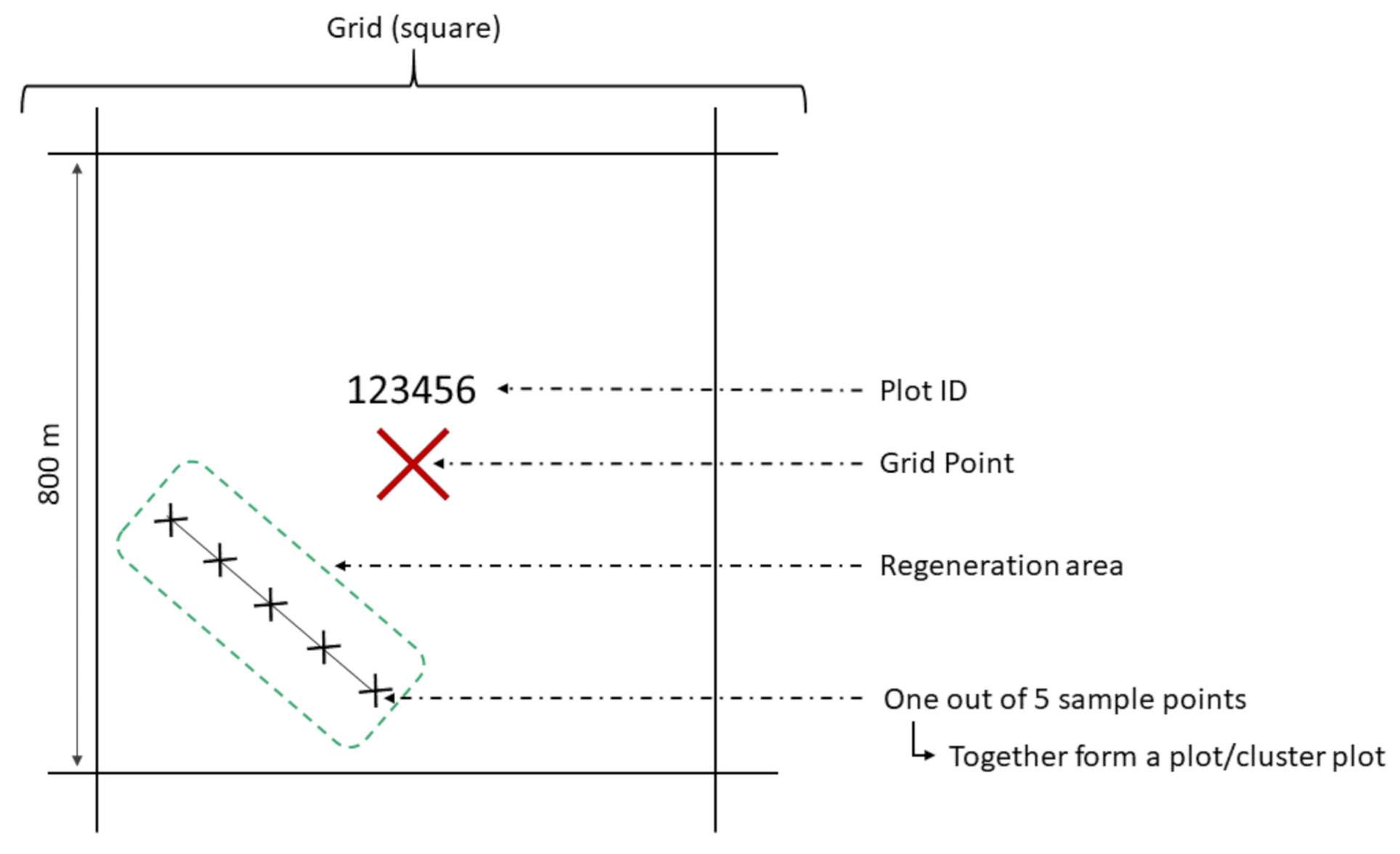
An 800 × 800 m (64 ha) mesh grid spanned across the entire BFNP area (see Figure 1 and Figure A9). Starting from the grid point, the closest regeneration area is identified. To avoid double counting, the regeneration area size should be at least 50 m in diameter and should have a regeneration density of more than 1300 plants ha−1 ≥ 20 cm. It was ensured that the leading shoots of the observed seedlings are still within reach of the locally occurring herbivores. In the BFNP, the maximal possible browsing height (considering the snow conditions in winter) is set at 200 cm. Measurements only take place on regeneration areas that meet these criteria. There is no grid where, due to the aforementioned requirements, no regeneration information is available.
To cover spatial browsing variation inside a regeneration area, a transect of at least 40 m (maximum 100 m) length is laid through the widest section of the regeneration area. Five sample points are mapped on the straight transect at intervals each corresponding to a quarter of the transect length. The first and the last sample points have to be at least 5 m away from the edge of the regeneration area. The coordinates in the center of the first sample point are recorded. Together, all sample points of a regeneration area form a (cluster) plot (see Figure 1). Each cluster plot is individualized by a plot ID [52,93]. Starting from the center of each sample point, the 15 closest individual seedlings are examined, which fulfill the height requirements (20–200 cm). The distance of the 15th recorded regeneration plant to the center of the sample point corresponds to the sample points’ radius. On each seedling inventoried, tree species and height are determined. To monitor the browsing injuries on the terminal shoot that occurred since the beginning of the last vegetation period, binary notation was used.
This standard procedure was extended by a separated regeneration inventory to increase the number of samples of rare tree species [94]. Tree species are classified as “rare” if they account for less than 5% of the total regeneration. In the BFNP, these are all of the tree species present with the exception of the Norway spruce and European beech species. At the centers of the sample points 2 and 4 of each transect, up to five of the closest “rare seedlings”, which are ≥20 cm and smaller than the maximum browsing height, are mapped at a maximum possible sample radius of 5 m.
Until 2010, about 400 plots per inventory were recorded. However, under the consideration of the inventory extension for rare tree species, the plot quantity was reduced to ca. 250 from 2011 onward [95].
2.4. Data Set
The data set contains the year of the respective inventory, the section of the BFNP, plot ID, consecutive number of sample points (1–5), consecutive number of observations (1–15), tree species, seedlings’ height and terminal shoot browsing (TRUE/FALSE).
We merged the data set of the standard regeneration inventories with the inventory extension. We took care to exclude double counting of rare tree species at the plot’s sample points 2 and 4. Therefore, we removed the rare tree species (all except spruce and beech) at the above-mentioned sample points from the standard inventory in all years from 2010 onward before merging the extended data. In total, there are 183,452 observations in our data set.
We took all tree species with a relative proportion of more than 0.5% in the data set (incorporating the inventory extension) into account in our analysis (compare, Appendix A.1). The tree species range includes Norway spruce, European beech, rowan, silver fir, birch (Betula spp.) and sycamore maple. Below this threshold, the quantity of seedlings was not sufficient to reliably determine browsing changes over a longer period of time.
2.5. Data Analysis
2.5.1. Browsing Probability and Its Change
Ungulate impact was predicted by estimating the odd-ratios of a single tree being browsed by using a generalized logistic mixed effect regression model (GLMM)—the browsing probability (BP) (question i) [6,26,96]. The logistic model used was chosen due to the binary nature of the single-tree browsing observations and to ensure that the resulting model estimates values between 0 and 1. We decided to apply a mixed model since the browsing observations clustered by every plot over time are expected to be stochastically dependent. As a fixed effect, we included year (of inventory) as a categorical variable (factor) with a fixed intercept and set a random intercept for the plot ID (see (1). The random intercept enhances the logistic model by adding a measurement repetition factor [97,98,99]. Furthermore, the random intercept serves as a surrogate for the possible effects of covariates that were not considered during data acquisition and, thus, not measured [97,98,100]. For example, browsing might depend on the altitude level and a plot can only be assigned to exactly one ecological altitude level. Such unobserved heterogeneity is therefore taken into account in our GLMM. In a previous model, we tried to account for possible BP variability between sample points nested in a plot in the random intercept. However, since this resulted in a decrease in model quality (Akaike information criterion) and since no or only a little variability was shown between sample points for many tree species, we have not pursued random intercept modification any further.
where
| = linear predictor for the browsing probability; | |
| = fixed intercept (the origin in our model); | |
| = cluster-specific (random) deviation from the fixed intercept; | |
| = random intercept for cluster (plot) i; | |
| = fixed slope parameter of covariate (year); | |
| = error term; | |
| = browsing probability. |
We estimated the BP for every tree species with the data set of the whole area of the BFNP and with the data set divided into its two management sections (FRG and RLG). Plot-level estimates are also potentially possible. Nonetheless, our analyses are carried out for the landscape and management unit scale since wildlife management decision making at the plot level would be impractical.
Subsequently, we formulated linear hypotheses for a simultaneous ANOVA procedure for each regression coefficient of the year j (see Equation (3)), tested them for significance and computed their 95% confidence intervals [96,101].
To estimate the changes in the BP based on the GLMM (question i), we modified the linear hypotheses (see Equation (4)). For each hypothesis, we took the difference between the regression parameters of the year j and the previous year of inventory . Testing the BP change over other time periods is, of course, also possible.
However, since the regression parameters are subtracted as logits, converting the BP change into a response (percentage) value afterwards is not possible.
2.5.2. Sensitivity Analysis
In seeking cost efficiency for the inventory method (question ii), we first determined the least number of observations of a tree species that must be present in the data set to maintain a significant change of BP between two years. This requires that a change was classified as significant in previous calculations. First, we divided the data set into two years in which the significant change was observed. Then, we ran a sensitivity analysis by using a Monte Carlo simulation, which iteratively reduced the total number of all seedlings across tree species. To achieve this, we simultaneously removed 20 random sample points in each iteration step from the data set between the years to be compared. Afterwards, we estimated the BP change with its confidence intervals for the respective tree species. We repeated this operation 1000 times for each step, to ensure that the estimations were based on different sample point combinations. For evaluation and graphical representation of the simulated values, we took the means of the logarithmic BP change in each iteration step (and their confidence intervals). The resulting minimum sample size marks the point at which the browsing change was last classified as significant. Between two data acquisition periods, the quantity of observed seedlings usually fluctuates. This difference between two years cannot be compensated by the simultaneous reduction in the samples. The minimum sample size always corresponds to the smallest sample size between each year.
In the results and appendix, only the tree species that represent more than 0.5% of the data set and that possess a significant BP change between the two most recent pairs of inventory years can be found (2012–2015 and 2015–2018). Assuming that the browsing probability estimates are more accurate due to a larger sample size, we used the data set of the BFNP as a whole.
2.5.3. Simulation of Ungulate Browsing
In the sensitivity analysis, we only worked with the assessed inventory data. Finding the minimum sample size for a significant BP change of a tree species was, therefore, limited to the actual observed browsing change. Theoretically, it could be possible that the applied inventory method is capable of detecting even smaller BP changes than observed in nature. To address question iii—to determine whether, for example, an increase in BP of exactly 2 percentage points (PP) for a tree species would represent a significant change—we generated data sets by simulating ungulate browsing that exactly reflect a certain change.
For this simulation we selected rowan because of its even distribution in the NP (throughout all altitude levels), its high amplitudes of BP and because it has the largest sample size among the rare tree species (compare Section 3.1 and Section 4.4). We used the most recent data from 2015 and 2018 for the simulation, as it represents the latest spatial distribution and abundance of rowan.
We left the browsing impact of the 2015 data set unchanged. For the year 2018, however, we set all browsing observations to “FALSE” to obtain a BP of 0%. In each simulation step, the simulation process randomly selects from the rowan 2018 data pool of five individuals. The selected individuals are then “browsed” by assigning the logic value “TRUE”. We then estimated the BP. As soon as the BP increased by ≥1 compared to 2015, the data set, with the individuals browsed by the simulation, was extracted and saved. This simulation sequence repeated for a BP increase of +1 to +15 PP in single absolute steps. The same sequence was modified to simulate a decrease in BP of −1 to −15 PP. Afterwards, we checked the change of BP for significance based on the generated data. The smallest and still significant change then equals the estimation accuracy for rowan of the currently applied inventory method in the BFNP. Finally, we applied the sensitivity analysis of Section 2.5.2 to the extracted data sets which were tested as significant. We could then examine the minimum number of observations needed for different estimation accuracies.
2.5.4. Computational Details
All calculations and simulations were executed by using R version 3.5.3 [102]. For the GLMM executions, we used the “lme4” package [98]. For testing the multiple linear hypothesis in consideration of simultaneous interference, we used the “multcomp” package [96]. All necessary editing of data structures and the graphical evaluation of all results of this work were performed with the package “tidyverse” [103].
3. Results
3.1. Browsing Probability Time Series
The detailed results of the BP and the BP change of the logistic mixed model of the respective tree species and NP region can be found in the Appendix A. To focus this work on the evaluation tool, only the highlights of the BFNP’s browsing probability times series are presented.
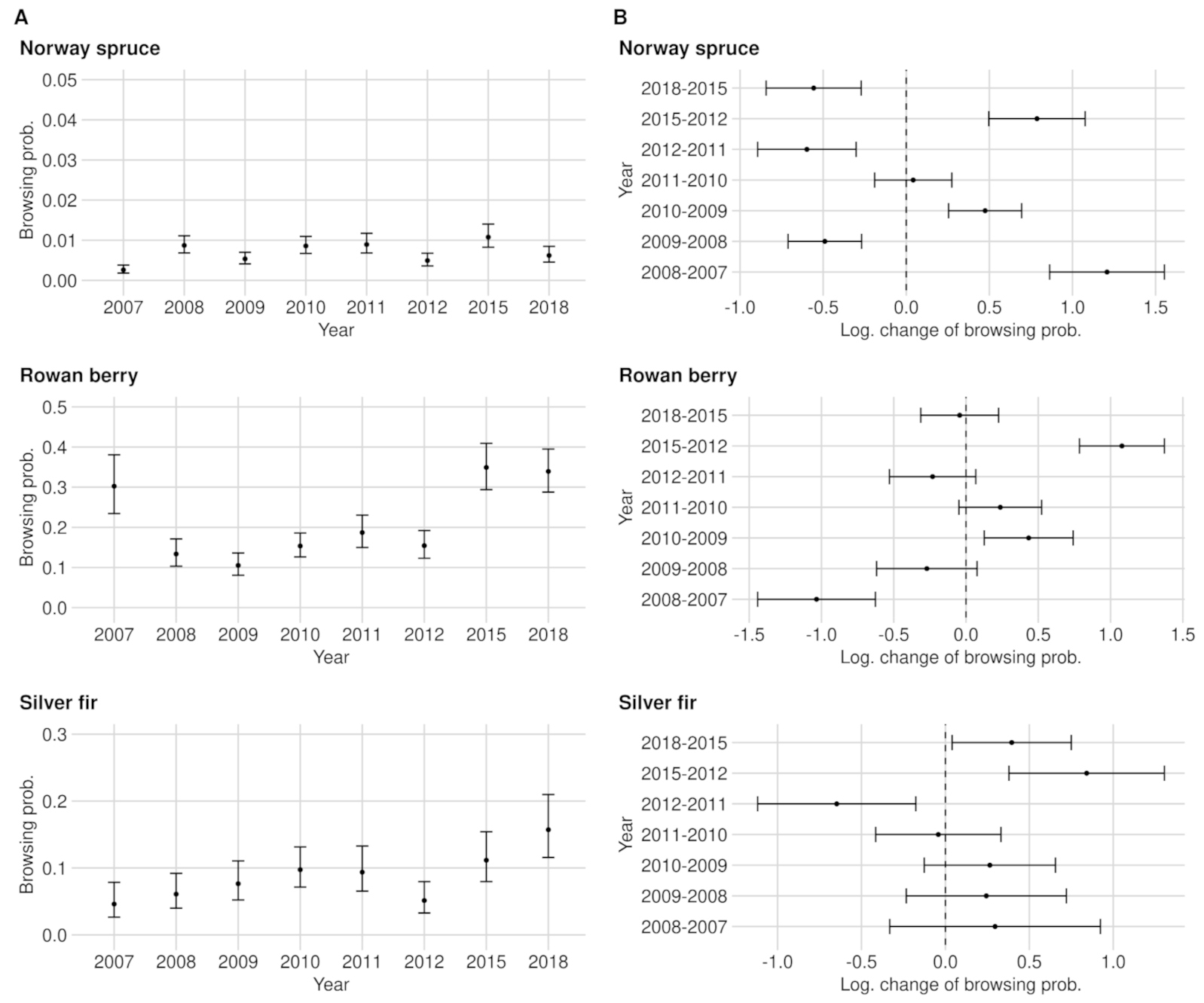
The BP levels between data acquisition years and tree species differ substantially. While the BP of the most frequent tree species (Norway spruce) never exceeded 1.1% (see Figure 2A), much higher BP levels and also BP amplitudes were found for rare broad-leafed tree species (see Appendix A). For instance the BPs of rowan berry fluctuate between 10.5% (2009) and 34.9% (2015) (see Figure 2A). Furthermore, we noted a trend that the rarer a tree species occurs in the NP (or the smaller the sample size), the less accurate the BP estimates become (or the wider the confidence intervals) (see Figure A4A). With few exceptions in tree species with a sparse sample size, the categorical expressions of variable year had a significant effect on the BP estimates (see Table A1).
To raise certainty that a BP change happened on the population level, we tested the logarithmic change of BP for significance (see Figure 2B and Figure A4). We found that the larger the sample size and the greater the BP change between years, the more likely a significant BP change could be detected (see Appendix A and Table A2). For instance, the lowest observed but still significant BP change in the entire NP is for rowan, which had an increase of +4.8 PP. For silver fir, although its sample size is slightly smaller than rowan, a BP change of +4.2% was observed (see Figure 2B). However, silver fir (ca. 8.5 obs. per plot with fir in 2018) is spatially more clumped compared to rowan (ca. 8 obs. per plot with rowan in 2018), which could explain the described phenomenon (compare Figure A10).
3.2. Significance of Changes and Sample Sizes
The simultaneous sample size reduction process demonstrated its flawless functionality. The smaller a sample size of a tree species became between two years, the more likely the once significant BP change became insignificant. We can reemphasize that the larger the sample size and the larger the observed significant BP change, the more observations could be removed from the sample size (see Appendix A.2). For example, we were able to reduce the sample size of Norway spruce by over 50% of its recorded sample size without losing significance for a BP change of +0.5 PP between 2015 and 2018 (see Figure A8). For the rare rowan berry tree species, we were able to reduce the sample size by ca. 80% for a BP change of +19.5 PP between 2012 and 2015 (see Figure A7).
3.3. Simulation of Ungulate Browsing on Rowan
We applied the browsing simulation on rowan only. Rowan is the most common rare tree species in the BFNP that sensitively reflects changes in ungulate browsing and it is spatially evenly distributed with a sufficient sample size (see Section 2.5.3 and Section 4.4.1 and Figure A10).
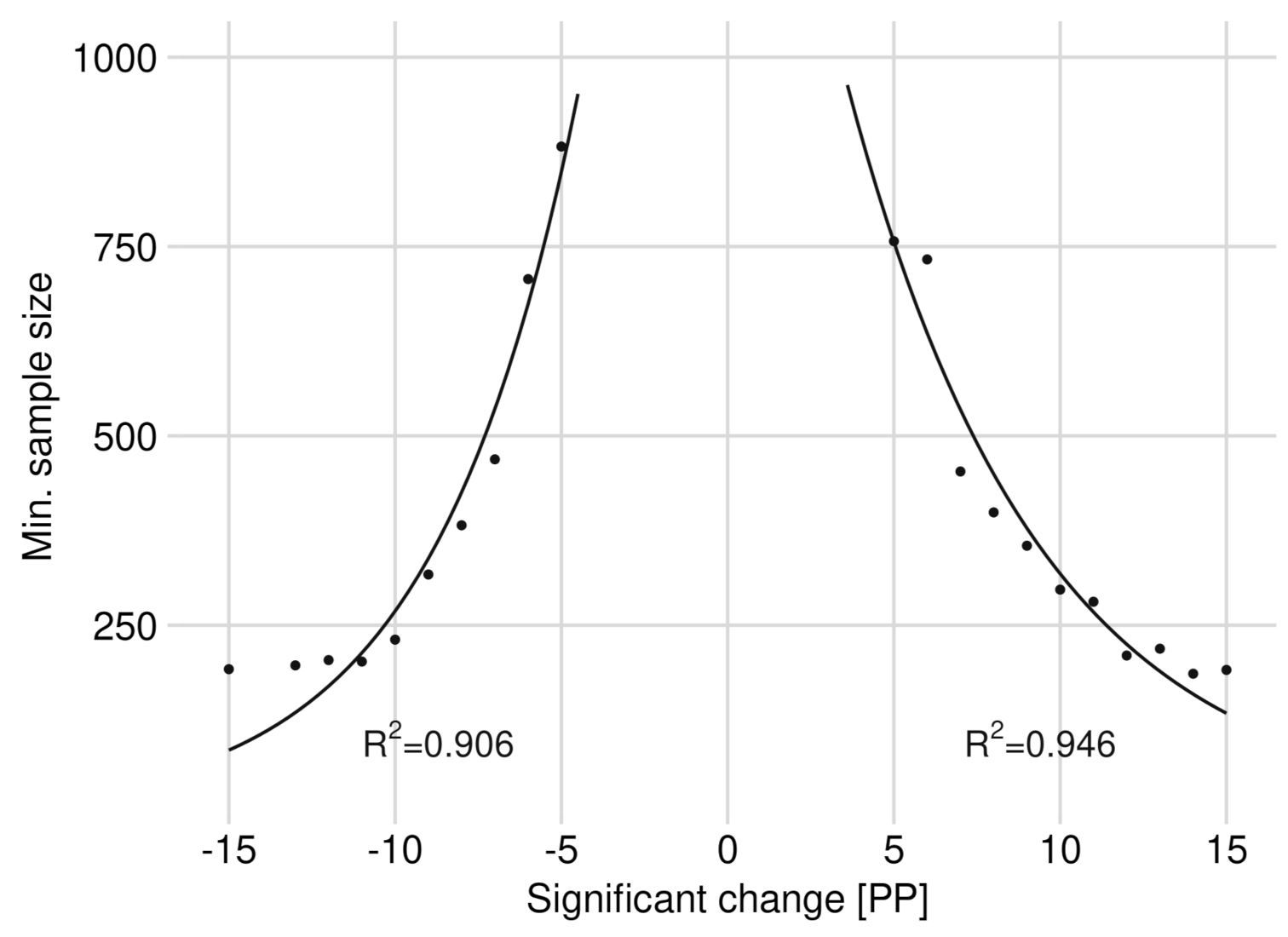
By increasing step-wise the BP of rowan in the 2018 data set by one percentage point each, starting from 34.9% (2015), we found a significant change starting from an increase of +5 PP (see Figure 3). The same BP change also results in a significant difference when we lowered the BP. We saved and provided data sets with the increased or decreased sample size for the following sensitivity analysis. The data sets contained the significant changes between ±5 PP and ±15 PP.
We were able to reduce the sample size for a significant increase in BP of +5 PP from 1007 to a minimum of 757 observations. A significant BP decrease of −5 PP required at least 882 observations. A minimum sample size of 399 (increase) or 382 (decrease) was required to observe a BP change by ±8 PP. For a significant BP change of ±15 PP, 192 observations (increase) or 191 (decrease) were required (see Figure 3).
The initially rapidly decreasing minimum sample size with increasing BP change must be emphasized. From a change of about ±9 PP, the decrease in the minimum sample size mitigates and remains relatively constant at a level above 200 observations. We were able to fit an exponential function from the minimum required sample sizes per BP change with a coefficient of determination of over 90% (see Figure 3). The estimated graphs of Figure 3 reflect their inflection point at a minimum sample size of ca. 350 observations. The exponential function for a significant BP decrease is listed in Equation (5) and for a BP increase in Equation (6).
4. Discussion
4.1. Evaluating Ungulate Browsing Impact (Question I)
The results show that calculating the BP with confidence intervals instead of the browsing intensity provides adaptive wildlife management with a better understanding of the accuracy of browsing predictions. Similar but rare approaches can be found by Kupferschmid et al. [26] and Hothorn et al. [96]. Morellet et al. [54] or Cederlund et al. [104], however, pointed out the importance of observing ecological changes for managing herbivore populations. A population level BP change, though, cannot be detected with certainty just by confidence interval widths of estimated BPs. Certainty about change is crucial when evaluating the success of wildlife management activities, e.g., with browsing thresholds [49,65,69].
Our example data set consists of 65% spruce observations. The estimates of BP and BP changes are correspondingly precise. Considering the low spruce BP compared to their browsing threshold of 12% [65], the estimation accuracy of the BP change is disproportionate to the effect it has on the spruce population. However, the closer a tree species reaches its respective browsing threshold, the more important it becomes to determine with certainty whether it exceeds it. For instance, we can observe in Figure 2A that the confidence intervals for the BP predictions of silver fir for the years 2011 and 2012 overlap. However, the significance test (Figure 2B) of the logarithmic change detects a significant reduction. While the 2011 BP estimate for silver fir exceeds the fir’s critical browsing threshold (of 9%), the 2012 estimate is below it. The silver fir example underlines the importance of a differentiated evaluation of statistically significant ungulate browsing changes to prevent false conclusions, enabling adaptive wildlife management.
4.2. The Ideal Sample Size and Cost Efficiency (Question II and III)
An ideal sample size depends on the resources of the organization conducting the inventory [105,106], the spatial distribution of the object of observation [107,108], the BP level [109] and the inventory objective. The sample size possesses indispensable information for the purposeful planning of sample-based inventory procedures [77], as it is decisive for the accuracy of an estimate. We measured the estimation accuracy in our results by the possibility of identifying a change of BP as significant. Our results outline that a higher sample size does not generally equal a higher estimation accuracy. For the spatially clumped silver fir, which has a slightly lower sample size than rowan and considerably lower BPs, we observed a significant BP change earlier than for rowan (see Section 3.3 and Appendix A.2.2, Figure A10).
As the estimation accuracy is altered by the site conditions in the inventoried area, the inventory method has to be designed so that an accuracy can be reached, which is suitable for the inventory’s objective—in our example, the state of forest regeneration [93]. The estimates must be precise enough to match browsing predictions and changes with the browsing thresholds of the tree species in focus [54]. Furthermore, a sufficient degree of estimation accuracy, especially for more rare tree species, is commonly counteracted by the limited resources of the inventory taker [105,106]. Therefore, inventory planning should always aim to achieve the maximum possible cost efficiency [105]. This can be accomplished either by achieving the highest possible accuracy with a fixed budget or by reducing the effort to the lowest possible level with fixed accuracy (compare [105,106,110,111]). Accordingly, we strive to find an ideal minimum sample size (as a guideline) for a desired level of accuracy based on the natural distribution of a species in our study site the BFNP.
Considering that the selectively browsed rowan could be a suitable browsing indicator tree species reflecting the management objectives of the BFNP (see Section 4.4.1), we based our browsing simulations and sensitivity analysis on its data set [68,112]. The results should provide an example of application of the simulation tool by using the most recent data from 2015 to 2018. We found the most cost-efficient minimum sample size of rowan to be ca. 350 observations for the BFNP with an accuracy for detecting changes between [−9:−8] and [8:9] (see Figure 3): Within this range, the minimum sample size decreases most effectively compared to the estimation accuracy since it marks the graph’s inflection point. In view of the annual BP fluctuations of rowan, the estimation accuracy of this cost-efficient sample size still seems sufficient.
However, as the ideal sample size is influenced by several conditions depending on the inventoried area, we recommend defining an inventory objective to which a desired estimation accuracy is linked. In the long term, the sample size could then be optimized to reach cost-efficiency and to define an ideal sample size with a comparable sensitivity analysis.
4.3. Inventory Design and Further Improvements
The data acquisition method used in the context of our study is based on the widely applied point-to-tree distance sampling technique (also known as k-tree or fixed count sampling) by Hothorn and Müller [6], Prodan [113], Kleinn and Vilčko [114], Staupendahl [115], Lynch and Rusydi [116], Picard et al. [117]. Distance sampling is known for its ease of application in the field; the amount of work remains constant at high stand densities, which are common on regeneration sites [115,116,117].
However, when working on distance sampled data, statistical challenges arise. Unbiased estimates of stand or regeneration densities require that the selection probability of all surveyed population elements in a plot design to be known [114,118]. The selection probability of an individual, using a distance sampling technique, depends on knowing the spatial distribution of its surrounding individuals [114,119]. Efforts required for calculating density-dependent selection probabilities of every acquired individual would make distance techniques impractical and are not usually provided [114,119]. Without incorporating selection-probabilities, absolute stand densities will be overestimated [114]. Relative browsing impact estimates are unlikely to be affected by sampling design bias. Nevertheless, the larger k is, the smaller the bias of estimates based on distance sampled data [114]. Therefore, a bias caused by distance sampling with , as in our case, is presumably not relevant and is outweighed by the ease of sampling.
However, the inventory method applied excludes all regeneration sites with a density lower than 1300 seedlings ha−1. This sets the selection probability of individuals occurring in areas with low regeneration density to zero. Kuijper et al. [120] and Churski et al. [121] both observed that ungulate browsing is clustered on high density regeneration sites in forest gaps. Consequently, the ungulate impact on the total regeneration of the BFNP might be overestimated with the current regeneration site selection rule. At the same time, the seedling selection is limited to individuals above 20 cm. The browsing pressure and the shift of competitive conditions of selectively browsed species starts from a seedling’s germination [6,122,123,124,125]. Therefore, the BP estimates could be left truncated. Moreover, the variable transect size (which varies between 40–100 m) alters the selection probability of seedlings again. Furthermore, the inventory method excludes the edges of regeneration sites due to its 5 m wide buffer zone (compare [93]). Clustered browsing on the edge of regeneration sites with a high density, such as observed by Čermák et al. [126], cannot be captured. The selection probabilities of rare tree species are further increased by the inventory extension. Hence the selection probability of a seedling, which is already hard to grasp when using a distance sampling technique, is further modified by multiple additional constraints which have only minimal practical advantages. In addition, the inventory extension falsifies statements about the relative species composition by increasing the sample size of rare tree species. Therefore, we could not consider the selection probability for the purposes of the application of our evaluation tool, for estimating BPs or their change applied in the BFNP example.
It is likely that our relative BP predictions are not biased by the applied distance sampling technique itself. Nevertheless, the inventory design is limited by the summed constraints. These constraints result in an unpredictable bias, reduces the comprehensibility of the inventory method and, therefore, reduce its acceptance. These issues could be easily resolved by fewer or no constraints on the inventory method. We want to highlight that the inventory method is only suitable to monitor ungulate browsing pressure; unbiased regeneration densities cannot be predicted, it only provides an impression about the proportions of the species composition and wildlife management must interpret the BPs as the upper limit of the observed area, as browsing pressure is likely to be higher on denser regeneration areas. Despite this criticism, regeneration inventories supporting landscape-scaled or enterprise-scaled wildlife management remain a rarity. In most cases, wildlife managers cannot refer to any data basis. Even if, from a statistical perspective, the inventory method requires improvement, it was sufficient from a practical stand-point for evaluating the ungulate impact on denser forest regeneration sites, thus, supporting adaptive wildlife management.
4.4. Opportunities for Future Research
4.4.1. Which Tree Species Must Undergo a Browsing Change to Trigger an Intervention in the Wildlife Population?
The results of the BP time series evaluation show how diversely individual tree species are affected by browsing (see Section 3.1 and Appendix A). Therefore, it is advisable that wildlife management decisions are based on browsing information of tree species that meet the overall management objectives of the considered forest area. These objectives may, for example, reflect forest owner-specific management interests [35,127] or be legally required, as in the BFNP. The most precise BP estimates in the BFNP example were obtained from spruce, which accounts for 65% of the observations in 2018. Due to its low palatability [19], spruce is not selectively browsed and, therefore, does not reflect the current browsing situation in the NP in terms of the total regeneration. For an inventory that aims for cost-efficiency, the high data acquisition effort cannot be justified for the evaluation of the browsing impact on spruce. Sycamore maple, on the other hand, is a selectively browsed tree species [125,128] and cannot provide reliable browsing results in the NP due to its low abundance of less than 1% in the data set. Alternatively, instead of increasing the global sample size, species could be identified that are selectively browsed and meet the inventory objective. In other words, browsing indicator species could be determined.
Even though an indicator species analysis is a common feature of ecological research (e.g., [129,130]), we were able to find just a few examples in forestry literature within the browsing context. For instance, Anderson [131] used Trillium grandiflorum as an indicator species to show the browsing intensity of the white-tailed deer (Odocoileus virginianus). Chevrier et al. [51] have observed how browsing intensity in young selectively browsed oak species (Quercus spp.) is related to the roe deer density in a 10 year series of experiments in France. From their observations they established an “oak browsing index”, which increased linearly with a high correlation to increasing roe deer densities. Furthermore, Morellet et al. [54] identified several indicator species to infer the size and performance of roe deer populations and their impact on the habitat to support an adaptive wildlife management.
However, using indicator species may result in a bias in favor of them, at the expense of other under-represented species [132]. To counteract this phenomenon, multiple requirements must be met to generate valuable information for adaptive wildlife management from indicator species. The following characteristics, which are modified and applied to wildlife management purposes according to Anderson [131], Carignan and Villard [106] and Williams et al. [133], stand out. The indicator species should:
- Act as an “early warning system” that reflects the influence of ungulate browsing of other tree species or, rather, a development of the ungulate densities in time;
- Be preferred by ungulates so that the indicator species sensitively indicates changes (large amplitude) rather than just indicating a change. Ideally, the species should be so sensitive that strong browsing quickly reduces its abundance;
- Be able to be monitored cost-efficiently; due to a high abundance and uniform distribution in the study area, an ideal browsing indicator species achieves a high estimation accuracy in data collection without great effort.
For the BFNP, rowan could be used as a well-fitting indicator species. Not only is a sufficient number of rowan available in the NP, but this species is also distributed evenly throughout the park to representatively observe browsing changes (see Figure A10). Rowan also seems to show changes of the browsing impact in the BFNP sensitively, which can be observed on its broad browsing amplitude (see Appendix A.1). Furthermore, rowan is considered a pioneer tree species and a biodiversity carrier [68,134] and, thus, it could meet the management objectives of the BFNP [46].
However, further application studies are needed to investigate the effect of adaptive wildlife management based on an indicator tree species on wildlife populations and forest regeneration. Moreover, inventory methods could be sought to efficiently study a indicator tree species.
4.4.2. From Which Browsing Probability or Threshold Does the Population of a Tree Species Decrease in the Long Run?
The correlation between browsing, loss of height increment and mortality has already resulted in the development of thresholds for the long-term permissible browsing intensity. These thresholds serve as a reference value for the respective tree species for wildlife management and are, therefore, of major importance (e.g., in the BFNP). However, the thresholds of Eiberle and Nigg [65,128] were determined based on 1363 observations in total, recorded at 23 different sites of the montane vegetation zone in the Swiss Alps. Accordingly, the estimated thresholds are only valid for this habitat and are not universally applicable without restriction. Additionally, they are limited to a small tree species spectrum. To the best of our knowledge, there is no further research to extend or update these thresholds. Only Kupferschmid et al. [25] recently documented a significant reduction in seedling stem numbers from a browsing probability between 5–10%. These observations relate to a wide range of different tree species that are also grown in Swiss mountain forests. Without comprehensive reference values, a regeneration inventory generates data without being able to evaluate it.
Light is often the most limited resource on the forest ground [39,135]. Compared to light, soil nutrients as well as water play a less important role for the growth of seedlings and saplings in most cases and in later stages in the temperate zone [3,136]. Under low light conditions and when the seedlings are already stressed, it is often not the one-time browsing that results in death but the repeated removal of the terminal shoot [19,65,137,138,139]. Non-selectively browsed seedlings gain an advantage in the competition for scarce light and can outcompete the browsed individuals—the so-called apparent competition [140]. Even if the primary shoot of a successively browsed tree grows out of ungulate reach, the competitive shift renders a subsequent death more likely [140,141]. These deer-plant, plant-environment interactions and tree-population dynamics should be taken into account when creating new browsing thresholds [60,64,135,142]. For this purpose, the development of sample trees, which forms the basis for the calculation of thresholds, has to be recorded spatially. The sample trees have to be placed into relation to the respective tree species and their height [64,135,142]. Such data acquisition, however, requires very high levels of effort since a very large spectrum of naturally growing species and mixture ratios has to be recorded over years. New three-dimensional forest development modeling approaches could help to better understand the tree population dynamics in combination with ungulate browsing (e.g., [135,141,142,143,144,145]). Individual survival probabilities (the likelihood to grow to an adult height) could then be calculated for specific tree species, affected by certain browsing probabilities and species constellations on a regeneration site.
5. Conclusions
Large-scale regeneration inventories have rarely been implemented in local adaptive wildlife management concepts and have seldom been the subject of research up to now. The Bavarian regeneration inventory, which was with minor modifications executed in the BFNP, is one of the first of its kind. Although it has room for methodical improvement, after little methodical adjustments of the inventory procedure, we can recommend the applied regeneration inventory as a base for adaptive wildlife management.
Browsing probabilities (BP) and their change computed by a generalized mixed effect model from periodically acquired regeneration data provide valuable information for wildlife management and underline the necessity of such inventories. Furthermore, estimating BPs instead of calculating the browsing intensity can significantly increase the credibility of regeneration inventories. Confidence intervals, which are mostly affected by the sample size and the local variability of the browsing impact, can be calculated, which further allows the detection of significant changes over time. BP changes can then be compared to browsing thresholds to estimate the effect of the change on the population of the tree species in focus. Our browsing time series clearly shows how much and how rapidly the ungulate impact can fluctuate. It also demonstrates how estimation accuracies can differ between tree species. A high degree of validity and credibility of the regeneration inventories are essential for wildlife management and for its public acceptance. Ungulates, which are managed based on such inventory reports, are a natural component of forest ecosystems; the forest is their livelihood. A regeneration inventory should be sufficiently precise to find a balance between forest regeneration and ungulates, improving the living conditions of the animals without compromising the objectives of silviculture and/or nature conservation.
The sensitivity analyses and the browsing simulations applied on a potential browsing indicator species show, that sample size could be reduced in favor of cost-efficiency and are still able to retrieve robust statements about the current browsing situation and its development. The analyses not only proved its high potential as a tool for saving inventory costs in the long term, but also demonstrated that an ideal sample size depends on several site dependent factors. Therefore, instead of defining an ideal or minimum sample size for targeted species, which is variable in every use case, we suggest determining a minimum estimation accuracy. A minimum estimation accuracy combined with an unambiguously formulated inventory aim would significantly increase the information value of a regeneration inventory and serve adaptive wildlife management as a reliable resource.
Author Contributions
Conceptualization, K.B. and M.H.; methodology, K.B.; software, K.B.; formal analysis, K.B.; investigation, K.B.; data curation, M.H.; writing—original draft preparation, K.B.; writing—review and editing, M.H., C.A. and T.K.; visualization, K.B.; supervision, M.H. and C.A.; project administration, M.H. and T.K.; funding acquisition, M.H. and T.K. All authors have read and agreed to the published version of the manuscript.
Funding
The research was funded by the program “Ziel ETZ Free State of Bavaria—Czech Republic 2014-2020 (INTERREG V)” and the German Federal Program “Biologische Vielfalt” by the German Federal Agency for Nature Conservation.
Acknowledgments
We thank the program Ziel ETZ Free State of Bavaria—Czech Republic 2014–2020 (INTERREG V) and the program “Biologische Vielfalt” for funding the present research. We would also like to thank Sennhenn-Reulen, who advised us and provided valuable tips with statistically driven questions. We are grateful to all the participants who acquired the browsing data in the Bavarian Forest National Park. Finally, we thank Alena Anderson Chilian and Juanita I. Schmidhammer for language editing and the anonymous reviewers for their valuable suggestions.
Conflicts of Interest
The authors declare no conflict of interest and the funders had no role in the design of the study; in the collection, analyses or interpretation of data; in the writing of the manuscript or in the decision to publish the results.
Abbreviations
The following abbreviations are used in this manuscript:
| BP | Browsing probability; |
| BFNP | Bavarian Forest National Park; |
| RLG | Rachel-Lusen region (in the Bavarian Forest National Park); |
| FRG | Falkenstein-Rachel region (in the Bavarian Forest National Park); |
| NP | National park; |
| Obs. | Observation; |
| PP | Percentage point. |
Appendix A. Detailed Browsing Evaluation of the BFNP
Appendix A.1. Browsing Probability Time Series
Appendix A.1.1. Norway Spruce
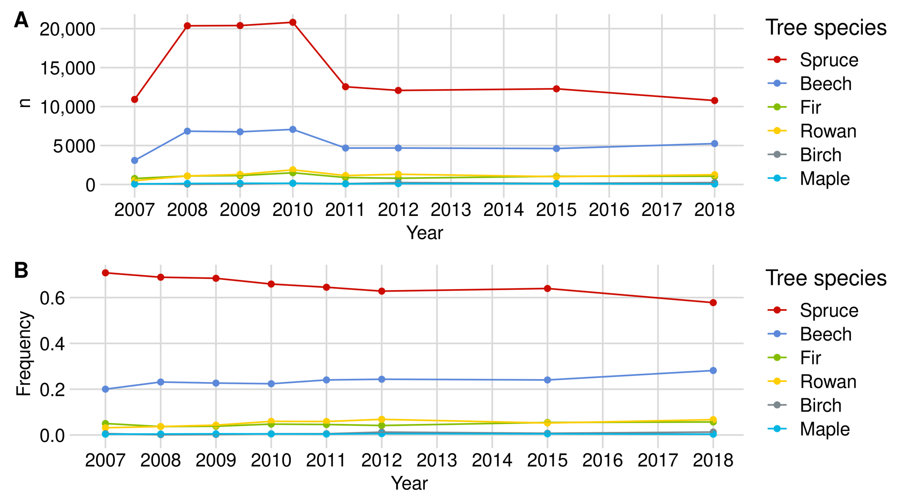
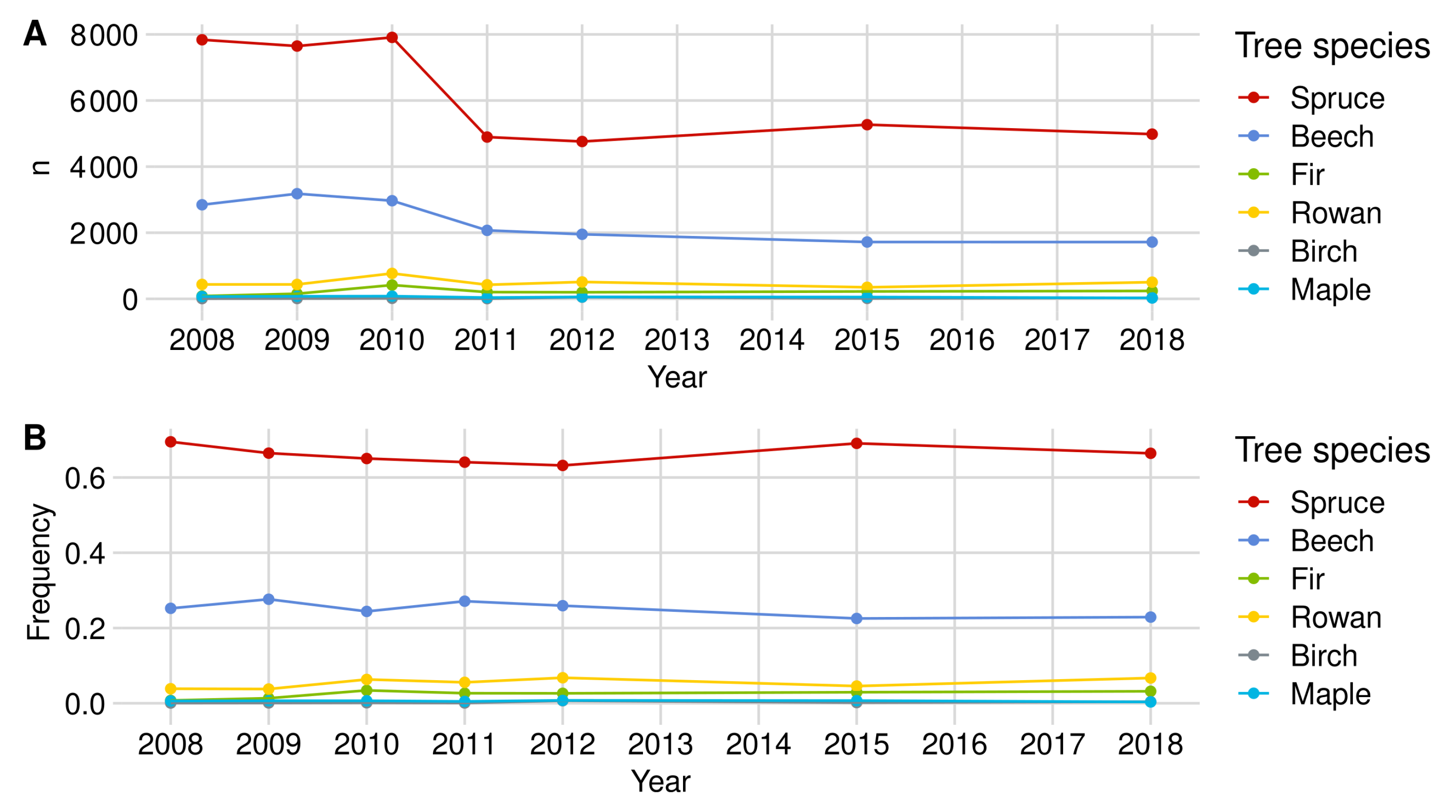
Norway spruce is the most common tree species in the regeneration data set. In the most recent regeneration inventory from 2018, 10,774 individuals were recorded throughout the NP (see Figure A1). Between 2010 and 2011, we observed a strong decrease in spruce individuals in both NP areas in our data set. This change is due to the optimization and thus reduction in the plot number in the regeneration inventory (see Section 2.3). However, the relative shares of spruce in relation to the total amount of regeneration in the NP in the respective year decreased from about 69% (2008) to 58% (2018).
Figure A1.
Sample size development of the main tree species over time in the NP in (A) total numbers (n) and (B) relative frequency.
Figure A1.
Sample size development of the main tree species over time in the NP in (A) total numbers (n) and (B) relative frequency.

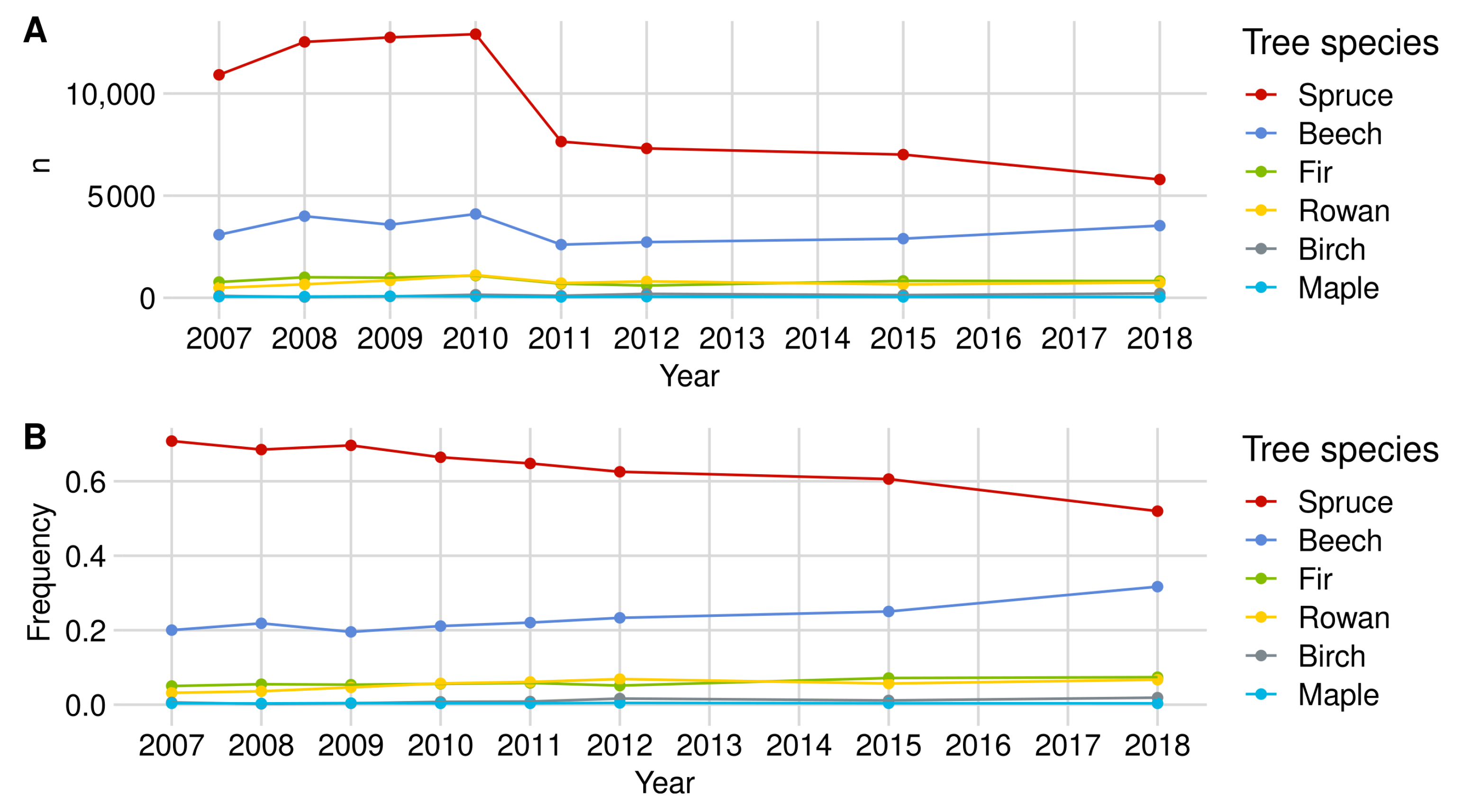
Figure A2.
Sample size development of the main tree species over time in the FRG in (A) total numbers (n) and (B) relative frequency.
Figure A2.
Sample size development of the main tree species over time in the FRG in (A) total numbers (n) and (B) relative frequency.

Figure A3.
Sample size development of the main tree species over time in the RLG in (A) total numbers (n) and (B) relative frequency.
Figure A3.
Sample size development of the main tree species over time in the RLG in (A) total numbers (n) and (B) relative frequency.

The BP over the entire NP corresponds to the average BP of RLG and FRG (see Figure A4A, Figure A5A and Figure A6A), although the RLG is slightly more dominant due to its sample size (see Figure A1 and Figure A3). The time series starts with a 0.3% BP identical to RLG since no inventory data were available for FRG in 2007 and remained relatively constant from 2008 onwards at about 0.9%. The strong increase in browsing probability in 2015 in FRG was also reflected in the evaluations of the entire NP. In 2015, spruce browsing culminated at approximately 1.1%. Moreover, the confidence interval width increased to ±0.3 PP, while the average width of all years was ±0.2 PP. In the most recent year, spruce BP was 0.6% with a 95%-confidence interval width of ±0.2 PP. Compared to all other tree species, spruce had the lowest browsing probability.
To raise certainty that a BP change happened on the population level, we tested the logarithmic change of BP for significance (Figure A4B). For spruce, all changes of the BP are significant apart from the difference between the years 2010 and 2011. The smallest significant change for the whole NP was +0.3 PP from 2009 to 2010.
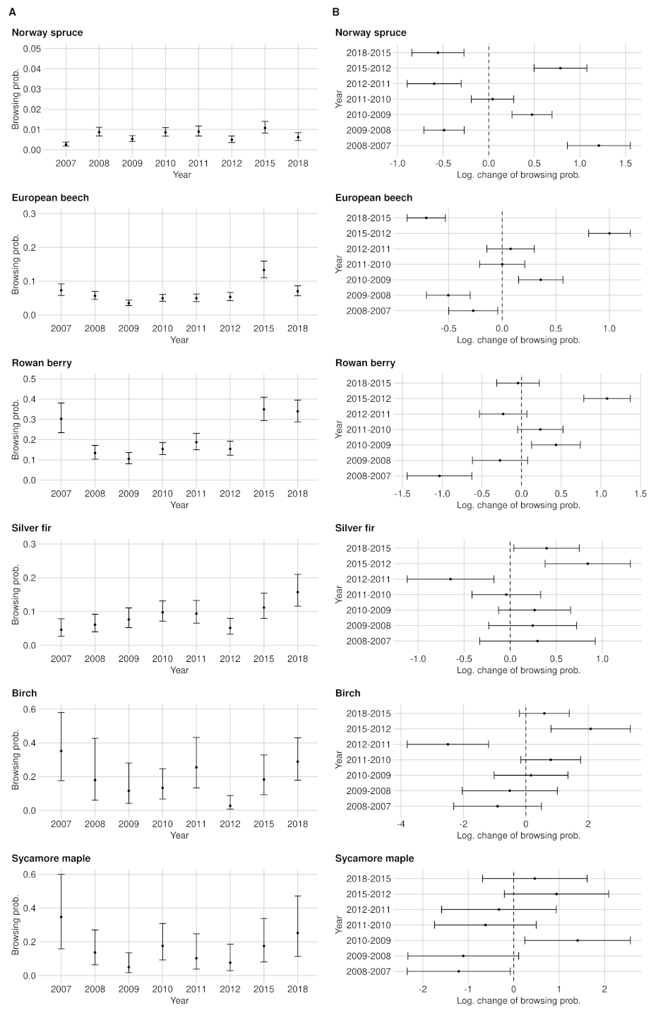
Figure A4.
Time series and confidence intervals of the BP (A) and the corresponding logarithmic change of the BP between two consecutive acquisition years (B). The estimated logarithmic change of BP (black point inside the confidence intervals) is positive if BP increased compared to the previous year, and is negative if it decreased. If either the upper or the lower end of the confidence intervals completely crossed the zero on the x-axis, the change of the BP is not significant. The estimates are related to the data set of the entire NP.

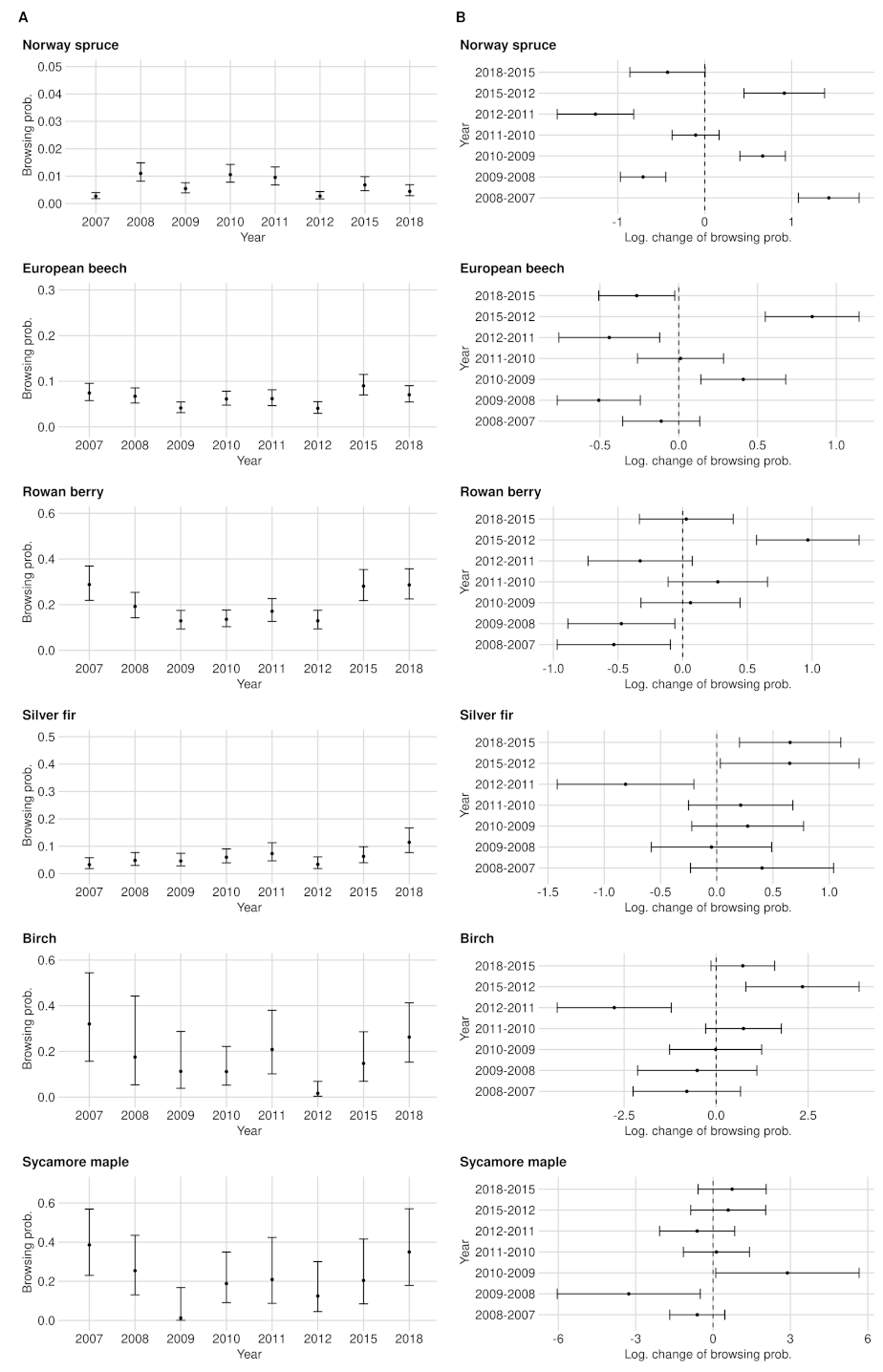
Figure A5.
Time series and confidence intervals of the BP (A) and the corresponding logarithmic change of the BP between two consecutive acquisition years (B). The estimated logarithmic change of BP (black point inside the confidence intervals) is positive if BP increased compared to the previous year, and is negative if it decreased. If either the upper or the lower end of the confidence intervals completely crossed the zero on the x-axis, the change of the BP is not significant. The estimates are related to the FRG data set.

Figure A6.
Time series and confidence intervals of the BP (A) and the corresponding logarithmic change of the BP between two consecutive acquisition years (B). The estimated logarithmic change of BP (black point inside the confidence intervals) is positive if BP increased compared to the previous year, and is negative if it decreased. If either the upper or the lower end of the confidence intervals completely crossed the zero on the x-axis, the change of the BP is not significant. The estimates are related to the RLG data set.


Table A1.
Summary statistics of all logistic mixed effect models for the respective tree species. Next to each categorical time step, logarithmic coefficients and the standard error (in parentheses) can be found.
Table A1.
Summary statistics of all logistic mixed effect models for the respective tree species. Next to each categorical time step, logarithmic coefficients and the standard error (in parentheses) can be found.
| Norway Spruce | European Beech | Rowan Berry | Silver Fir | Birch | Sycamore Maple | |
|---|---|---|---|---|---|---|
| 2007 | −5.94 *** | −2.54 *** | −0.84 *** | −3.03 *** | −0.61 | |
| 2008 | −4.73 *** | −2.81 *** | −1.87 *** | −2.74 *** | −1.52 *** | −1.84 *** |
| 2009 | −5.22 *** | −3.31 *** | −2.14 *** | −2.49 *** | −2.03 *** | −2.95 *** |
| 2010 | −4.75 *** | −2.95 *** | −1.71 *** | −2.23 *** | −1.87 *** | −1.54 *** |
| 2011 | −4.71 *** | −2.95 *** | −1.47 *** | −2.27 *** | −1.07 *** | −2.17 *** |
| 2012 | −5.31 *** | −2.88 *** | −1.70 *** | −2.92 *** | −3.57 *** | −2.49 *** |
| 2015 | −4.52 *** | −1.87 *** | −0.62 *** | −2.07 *** | −1.49 *** | −1.55 *** |
| 2018 | −5.08 *** | −2.58 *** | −0.67 *** | −1.68 *** | −0.90 *** | −1.08 ** |
| AIC | 16,925.02 | 21,784.74 | ||||
| BIC | 17,012.29 | 21,862.76 | ||||
| Log Likelihood | −8453.51 | −10,883.37 | −4412.72 | −2471.14 | −481.87 | −353.87 |
| Num. obs. | 120,164 | 42,979 | 9474 | 8313 | 1117 | 850 |
| Num. groups: PlotID | 412 | 343 | 370 | 254 | 132 | 76 |
| Var: PlotID (Intercept) |
*** p < 0.001; ** p < 0.01.
Table A2.
Summary statistics of the multiple comparisons of means between year levels for the respective tree species. Next to each categorical time step, logarithmic coefficients and the standard error (in parentheses) can be found.
Table A2.
Summary statistics of the multiple comparisons of means between year levels for the respective tree species. Next to each categorical time step, logarithmic coefficients and the standard error (in parentheses) can be found.
| Norway Spruce | European Beech | Rowan Berry | Silver Fir | Birch | Sycamore Maple | |
|---|---|---|---|---|---|---|
| 2008–2007 | 1.208 *** | −0.27 * | −1.034 *** | −1.209 * | ||
| 2009–2008 | −0.49 *** | −0.503 *** | ||||
| 2010–2009 | 0.474 *** | 0.36 *** | 0.434 ** | 1.406 ** | ||
| 2011–2010 | ||||||
| 2012–2011 | −0.598 *** | −0.647 ** | −2.499 *** | |||
| 2015–2012 | 0.786 *** | 1.001 *** | 1.079 *** | 0.842 *** | 2.077 *** | |
| 2018–2015 | −0.557 *** | −0.708 *** | 0.395 * | |||
| 2018–2008 | −0.342 ** | 0.229 * | 1.203 *** | 1.056 *** | ||
*** p < 0.001; ** p < 0.01; * p < 0.05.
Appendix A.1.2. European Beech
With a share of 24%, beech is the second most common tree species in the regeneration data set (see Figure A1). The evaluations from 2018 were based on 5250 beech seedlings and seedlings of which about one-third were in FRG and two-thirds in RLG (see Figure A2 and Figure A3). As in the case of spruce, a lower number of beech trees were observed from 2010 onward due to the reduction in the plot numbers (see Figure A1).
The estimated BP of beech is considerably higher compared to spruce. BP had its minimum of 3.5% in 2009 and its maximum of 13.3% in 2015. While the confidence intervals in 2015 ranged around the estimate by ±2.7 PP, they were ±1.5 PP wide on average (see Figure A4A). From 2010 to 2011 (+1.4 PP) and from 2011 to 2012 (±0.0 PP), we could not detect any significant browsing changes in the entire NP area. The lowest observed and still significant change of BP was found between 2009 and 2010 with an increase of +1.4 PP (see Figure A4B).
Appendix A.1.3. Rowan Berry
The rowan is the most frequently observed rare tree species over all years. Observations numbering 1251 were available in 2018, which make up 6.7% of the data set. Only in 2007 and 2015 was silver fir the more frequent rare tree species in the NP (see Figure A1). In 2018, the rowan had about the same share in the regeneration data set in both NP subregions (see Figure A5 and Figure A6). The inventory extension for rare tree species from 2010 onward (see Section 2.5.1) and the optimization of the plot number are quantitatively noticeable in the rowan data set. Due to the inventory extension, the share of rare tree species in the total regeneration data is distorted so that we cannot observe any trends here.
Rowan was browsed significantly more than spruce or beech. Between 2007 and 2012, the BP fluctuated between 10.5% (2009) and 18.7% (see Figure A4A). From 2010 onward, we noticed a continuous increase in BP, culminating in 2015 with 34.9%. Here, the relatively low BP of 28.1% in RLG in 2015 could compensate for the high BP in FRG of approximately 47% (see Figure A5 and Figure A6). In 2018, we estimated the probability of a rowan to be browsed at 33.9%. At about ±4.1 PP, the confidence intervals ranged around the estimates.
In between the years of 2007–2008, 2009–2010 and 2012–2015, we measured a significant change in BP. The lowest observed but still significant BP change in the NP was shown between 2009 and 2010 with an increase of +4.8 PP (see Figure A4B).
Appendix A.1.4. Silver Fir
With around 1062 observations in 2018, silver fir is the second most common rare tree species in the data set (inventory extension included (see Figure A1). The relative share of fir in the regeneration data set has constantly been rising from 2010. Nevertheless, it does not correspond to the share of actual regeneration since the inventory extension raises the fir sample size (see Section 2.5.1). In direct comparison, significantly more fir trees were mapped in RLG in 2018 than in FRG—823 (77.5%) to 239 (22.5%) (see Figure A2 and Figure A3).
Up to and including 2012, the BP of fir in the entire NP remained below 10%. The BP more than doubled from 5.1% to 11.2% only from 2012 to 2015. Due to the increase in BP in RLG towards 2018 (11.5%) and the already high values in FRG (27.6%), a further increase to 15.7% was observed in the entire area from 2015 to 2018 (see Figure A5 and Figure A6). On average, the confidence intervals surround the BP estimate ±2,6% (see Figure A4A).
From 2011 on, we were able to address all BP changes with a safe 95% confidence interval for the entire NP as well as for the RLG. The smallest and still significant BP change is +4.2% (from 2012 to 2015), while in the RLG, a change of +2.9% (from 2012 to 2015) is still significant despite a smaller sample size(see Figure A4B, Figure A5 and Figure A6).
Appendix A.1.5. Birch
Birch trees are the third most common rare tree species group (including the inventory extension) in the NP’s data set. Observations numbering 241, which correspond to a share of 1.3% in our data set, are included for our BP estimation in 2018. Of the 241 seedlings (2018), 210 (87%) were in RLG and 31 (13%) in FRG (see Figure A1, Figure A2 and Figure A3). Due to the spatial dominance of birch in RLG, the BP estimates for the total NP largely correspond to those of the RLG. For the same reason, it is not possible to make any statements about the development of browsing in FRG.
Ungulate browsing on birch was strongly fluctuating over time in RLG. In 2007, the time series started with the maximum BP value of 32% and decreased to 11.1% in 2010 but doubled in 2011. In 2012, we observed a strong decrease in the browsing probability to 1.6% and an increase in 2018 to 26.3%. Similar to the fluctuating BP, the confidence interval widths were also fluctuating between ±3.3 PP (2012) and ±19, PP (2008) (see Figure A4A, Figure A5 and Figure A6).
Appendix A.1.6. Sycamore Maple
Sycamore maple is the fourth rarest tree species in the NP (with inventory extension). With 67 observations, the tree species accounts for about 0.4% of the examined regeneration in 2018. The number as well as the percentage of observed sycamore trees seemed to decrease until 2012. In contrast to the rare tree species described above, the share of sycamore maple in the regeneration data set of the respective sub-area is balanced at approximately 0.4% in RLG and FRG in 2018 (see Figure A1, Figure A2 and Figure A3).
Between 2008 and 2018, we estimated sycamore maple probabilities of BP in the NP area between 5% (2009) and 25.3% (2018). From 2012 onward, we identified a steadily increasing BP. On average, the confidence interval width was about ±12.3 PP wide (see Figure A4A). Only the increase in BP in the entire NP by +12 PP from 2009 to 2010 was significant. While we also measured the change between 2008 and 2009 in the RLG as significant, we did not observe any significant change in the FRG (see Figure A4B, Figure A5 and Figure A6).
Appendix A.2. Significance of Changes and Sample Sizes
Appendix A.2.1. Significant Changes of BP between 2012 and 2015
We confirmed the increase in spruce’s BP of +0.6 PP in Appendix A.1.1 as significant. The estimation was based on 12,073 seedling observations in 2012 and 12,280 in 2015. We were able to reduce the sample size down to 5008 individuals without losing significance once, which was observed at the excess of the zero threshold of the confidence interval boundaries. Below 5008 observations, we sometimes observed a loss of significance. From approximately less than 3600 individuals, the significance loss incidence becomes regular (see Figure A7).
Between 2012 (4680 observations) and 2015 (4615 observations), the BP of beech rose significantly by +8 PP (see Appendix A.1.2). The observed change was so distinct that the sample size reduction was not able to break the significance. If we reduced the sample size below 992 beech seedlings, the sensitivity analysis was terminated by multiple error messages, which implied that the sample size per plot was too low (see Figure A7).
Between 2012 (1315 observations) and 2015 (1007 observations), we observed a change of BP of rowan by +19.5 PP (Appendix A.1.3). Within the sensitivity analysis, we were able to reduce the minimum sample size to 198 without losing significance until the analysis process was aborted by the same error messages as mentioned above (see Figure A7).
For silver fir, BP doubled from 2012 (799 observations) and 2015 (1053 observations) by +6.1 PP (see Appendix A.1.4). We were able to observe this significant change until a minimum sample size of 189 seedlings (see Figure A7).
Between 2012 and 2015, the estimated BP of birch increased six-fold from 2.7% (based on 243 observations) to 18.3% (based on 146 observations) (see Appendix A.1.5). After reducing the sample size to approximately 95 (0.4 birch trees per plot), BP lost significance (see Figure A7).
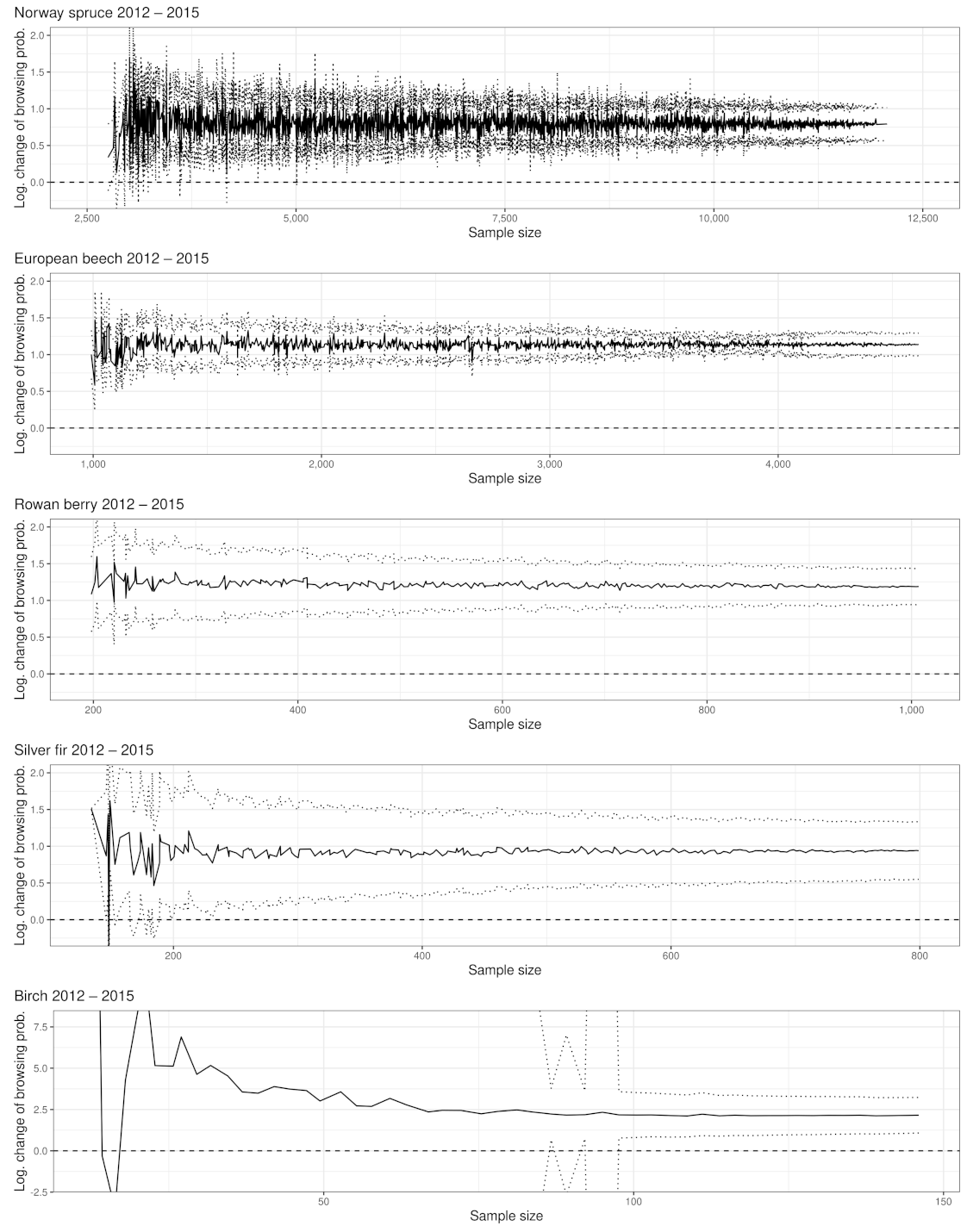
Figure A7.
The results of the sensitivity analysis for the BP change of all tree species for which its change was as significant between 2012 and 2015. On the x-axis, the sample size and the estimates of the confidence intervals (dashed) of the logarithmic BP change on the y-axis.
Figure A7.
The results of the sensitivity analysis for the BP change of all tree species for which its change was as significant between 2012 and 2015. On the x-axis, the sample size and the estimates of the confidence intervals (dashed) of the logarithmic BP change on the y-axis.

Appendix A.2.2. Significant Changes of BP between 2015 and 2018
The BP of spruce regeneration decreased from 2015 (12,280 observations) to 2018 (10,774 observations) by −0.5 PP (see Appendix A.1.1). We ware able to eliminate observations to a sample size of 5020 without losing significance (see Figure A8).
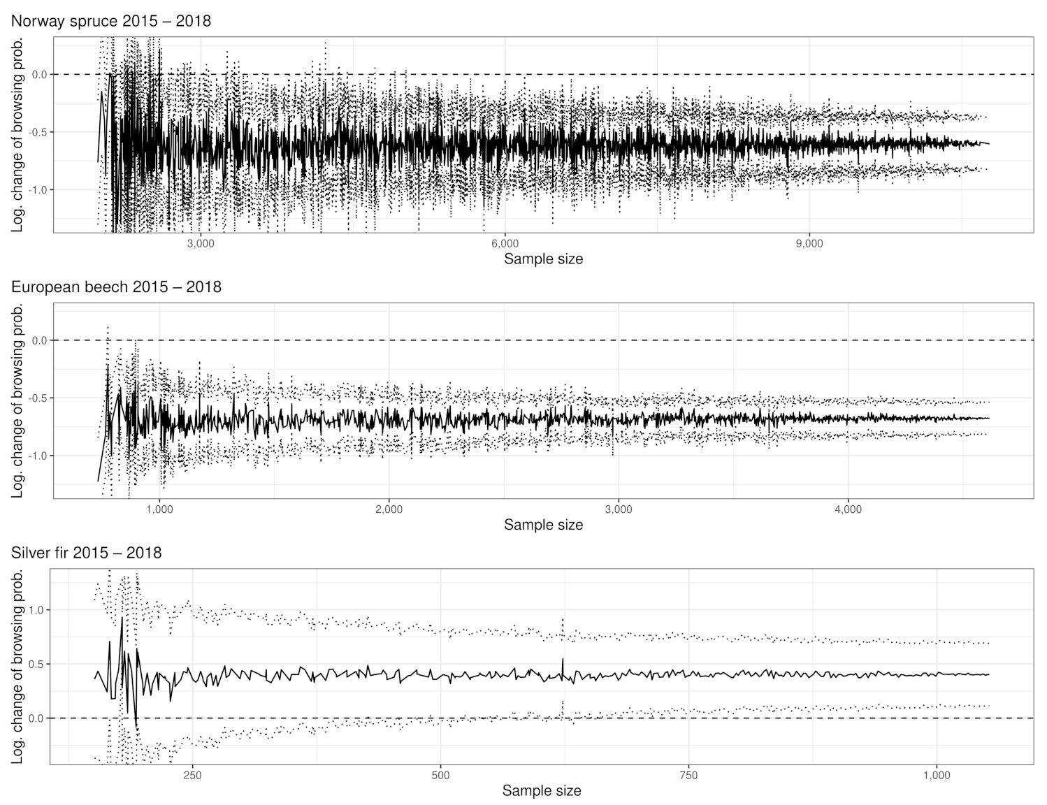
Figure A8.
The results of the sensitivity analysis for the BP change of all tree species for which its change was tested as significant between 2015 and 2018. The sample size is on the x-axis and the estimates of the confidence intervals (dashed) of the logarithmic BP change is on the y-axis.
Figure A8.
The results of the sensitivity analysis for the BP change of all tree species for which its change was tested as significant between 2015 and 2018. The sample size is on the x-axis and the estimates of the confidence intervals (dashed) of the logarithmic BP change is on the y-axis.

The change of BP of beech (−6.3 PP between 2015 (4615 seedlings) and 2018 (5250 seedlings)) was measured as significant (Appendix A.1.1). With our sample size reduction, it was only possible to lose significance twice; significance was lost once with a sample size of 895 and once with a sample size of 775 before aborting our computing processes after the error messages reported above (see Figure A8). The occurrence of the two significance losses can be explained by a random combination of the removed sample points and can be interpreted as outliers.
Moreover, for silver fir, we found a significant BP change of +4,6 PP between 2015 (1053 individuals) and 2018 (1062 individuals) (see Appendix A.1.4). The significance remained at a sample size for 679 observations. Thereafter, the lower half of the confidence interval regularly crosses the significance boundary (see Figure A8).
Appendix B. Figures
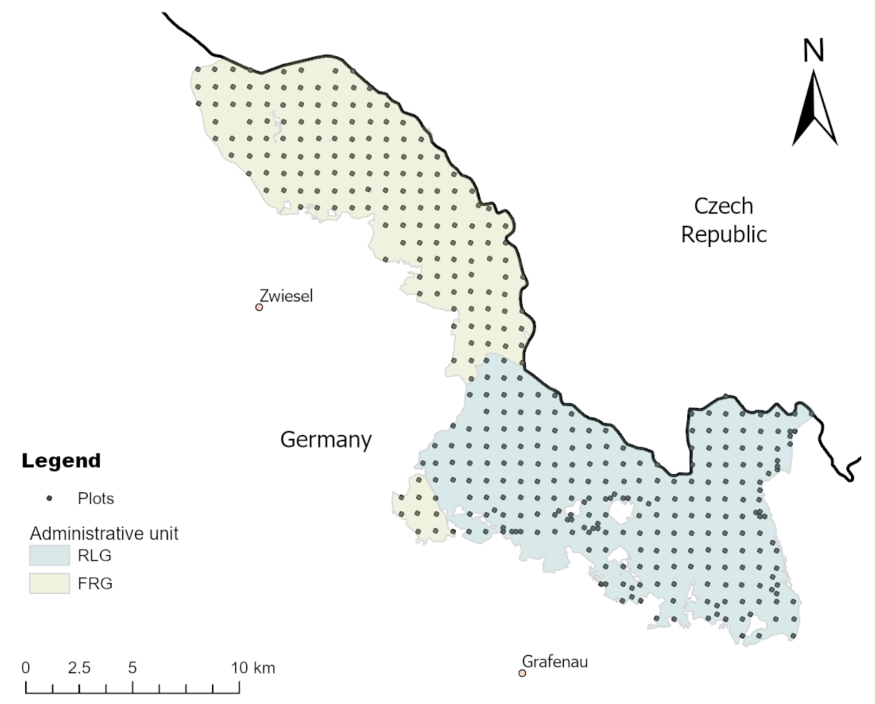
Figure A9.
Overview of the administrative organization of the study area (Bavarian Forest National Park); RLG = Rachel-Lusen-Region (light blue); FRG = Falkenstein-Rachel-Region (light green); systematic distributed plots of the regeneration inventory. The few plots which fall out of that grid near the NP’s borders are not incorporated in our analysis.

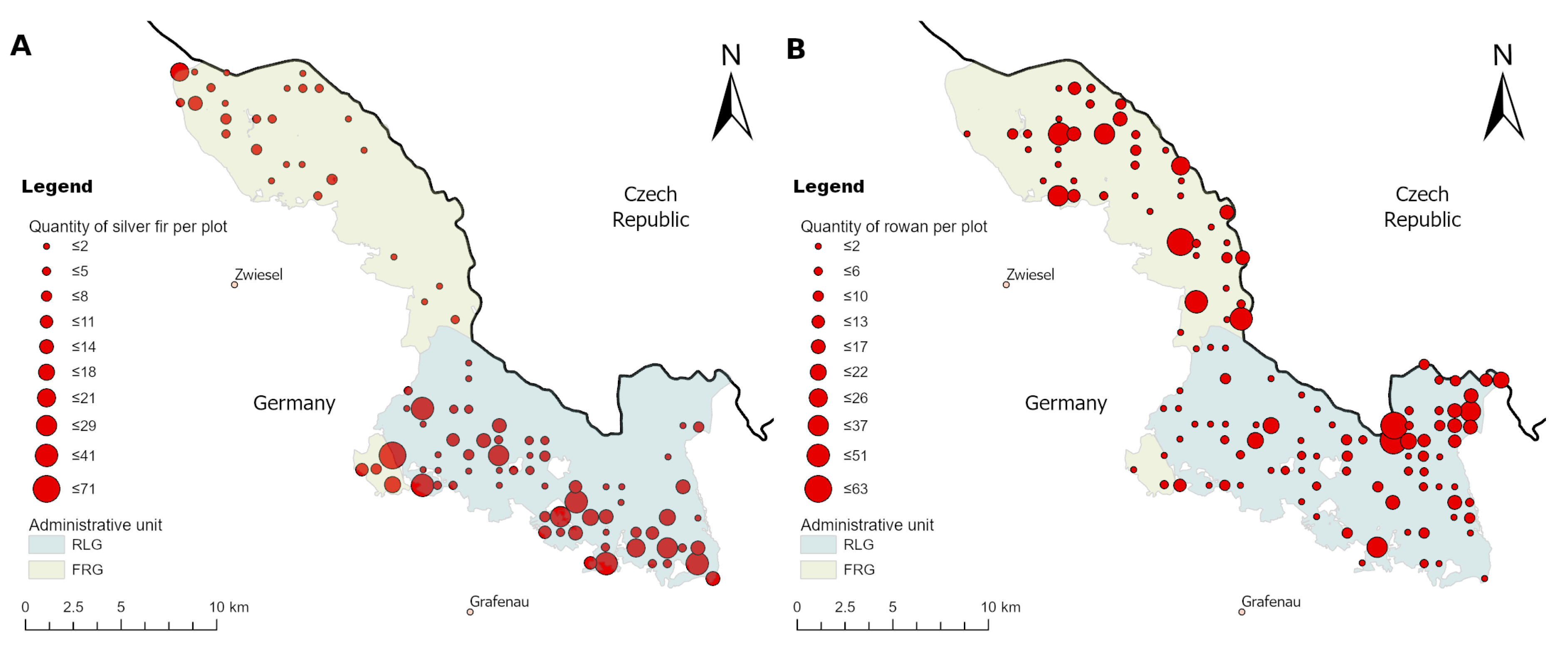
Figure A10.
Spatial distribution of the silver fir (A) and the rowan (B) in our study area.

References
- Terborgh, J. Ecological Meltdown in Predator-Free Forest Fragments. Science 2001, 294, 1923–1926. [Google Scholar] [CrossRef] [Green Version]
- Pastor, J.; Cohen, Y. Herbivores, the Functional Diversity of Plants Species, and the Cycling of Nutrients in Ecosystems. Theor. Popul. Biol. 1997, 51, 165–179. [Google Scholar] [CrossRef]
- Gill, R.M.A. A Review of Damage by Mammals in North Temperate Forests: 3. Impact on Trees and Forests. Forestry 1992, 65, 363–388. [Google Scholar] [CrossRef] [Green Version]
- Möst, L.; Hothorn, T.; Müller, J.; Heurich, M. Creating a Landscape of Management: Unintended Effects on the Variation of Browsing Pressure in a National Park. For. Ecol. Manag. 2015, 338, 46–56. [Google Scholar] [CrossRef]
- Peringer, A.; Schulze, K.A.; Stupariu, I.; Stupariu, M.S.; Rosenthal, G.; Buttler, A.; Gillet, F. Multi-Scale Feedbacks between Tree Regeneration Traits and Herbivore Behavior Explain the Structure of Pasture-Woodland Mosaics. Landsc. Ecol. 2016, 31, 913–927. [Google Scholar] [CrossRef]
- Hothorn, T.; Müller, J. Large-Scale Reduction of Ungulate Browsing by Managed Sport Hunting. For. Ecol. Manag. 2010, 260, 1416–1423. [Google Scholar] [CrossRef]
- Fuller, R.J. Responses of Woodland Birds to Increasing Numbers of Deer: A Review of Evidence and Mechanisms. Forestry 2001, 74, 289–298. [Google Scholar] [CrossRef]
- Ammer, C. Impact of Ungulates on Structure and Dynamics of Natural Regeneration of Mixed Mountain Forests in the Bavarian Alps. For. Ecol. Manag. 1996, 88, 43–53. [Google Scholar] [CrossRef]
- Ripple, W.J.; Newsome, T.M.; Wolf, C.; Dirzo, R.; Everatt, K.T.; Galetti, M.; Hayward, M.W.; Kerley, G.I.H.; Levi, T.; Lindsey, P.A.; et al. Collapse of the World’s Largest Herbivores. Sci. Adv. 2015, 1, e1400103. [Google Scholar] [CrossRef] [Green Version]
- Apollonio, M.; Andersen, R.; Putman, R. (Eds.) European Ungulates and Their Management in the 21st Century; Cambridge University Press: Cambridge, UK; New York, NY, USA, 2010. [Google Scholar]
- Bradshaw, R.H.; Hannon, G.E.; Lister, A.M. A Long-Term Perspective on Ungulate–Vegetation Interactions. For. Ecol. Manag. 2003, 181, 267–280. [Google Scholar] [CrossRef]
- Milner, J.M.; Bonenfant, C.; Mysterud, A.; Gaillard, J.M.; Csanyi, S.; Stenseth, N.C. Temporal and Spatial Development of Red Deer Harvesting in Europe: Biological and Cultural Factors. J. Appl. Ecol. 2006, 43, 721–734. [Google Scholar] [CrossRef]
- Linnell, J.D.; Cretois, B.; Nilsen, E.B.; Rolandsen, C.M.; Solberg, E.J.; Veiberg, V.; Kaczensky, P.; Van Moorter, B.; Panzacchi, M.; Rauset, G.R.; et al. The Challenges and Opportunities of Coexisting with Wild Ungulates in the Human-Dominated Landscapes of Europe’s Anthropocene. Biol. Conserv. 2020, 244, 108500. [Google Scholar] [CrossRef]
- Ripple, W.J.; Estes, J.A.; Beschta, R.L.; Wilmers, C.C.; Ritchie, E.G.; Hebblewhite, M.; Berger, J.; Elmhagen, B.; Letnic, M.; Nelson, M.P.; et al. Status and Ecological Effects of the World’s Largest Carnivores. Science 2014, 343. [Google Scholar] [CrossRef] [Green Version]
- Ammer, C.; Vor, T.; Knoke, T.; Wagner, S. Der Wald-Wild-Konflikt: Analyse Und Lösungsansätze Vor Dem Hintergrund Rechtlicher, Ökologischer Und Ökonomischer Zusammenhänge. In Göttinger Forstwissenschaften; Niedersächsische Staats-und Universitätsbibliothek and Univ. Verl. Göttingen: Göttingen, Germany, 2010; Volume 5. [Google Scholar]
- Boulanger, V.; Baltzinger, C.; Saïd, S.; Ballon, P.; Picard, J.F.; Dupouey, J.L. Ranking Temperate Woody Species along a Gradient of Browsing by Deer. For. Ecol. Manag. 2009, 258, 1397–1406. [Google Scholar] [CrossRef]
- Eiberle, K. Über Den Einfluss Des Wildverbisses Auf Die Mortalität von Jungen Waldbäumen in Der Oberen Montanstufe. Schweiz. Z. Forstwes 1989, 140, 1031–1042. [Google Scholar]
- Rooney, T.P. Deer Impacts on Forest Ecosystems: A North American Perspective. Forestry 2001, 74, 201–208. [Google Scholar] [CrossRef] [Green Version]
- Vavra, M.; Parks, C.G.; Wisdom, M.J. Biodiversity, Exotic Plant Species, and Herbivory: The Good, the Bad, and the Ungulate. For. Ecol. Manag. 2007, 246, 66–72. [Google Scholar] [CrossRef]
- Gill, R.M.A. A Review of Damage by Mammals in North Temperate Forests: 1. Deer. Forestry 1992, 65, 145–169. [Google Scholar] [CrossRef] [Green Version]
- Bergquist, J.; Bergström, R.; Zakharenka, A. Responses of Young Norway Spruce (Picea Abies) to Winter Browsing by Roe Deer (Capreolus Capreolus): Effects on Height Growth and Stem Morphology. Scand. J. For. Res. 2003, 18, 368–376. [Google Scholar] [CrossRef]
- Harmer, R. The Effect of Plant Competition and Simulated Summer Browsing by Deer on Tree Regeneration. J. Appl. Ecol. 2001, 38, 1094–1103. [Google Scholar] [CrossRef]
- Kupferschmid, A.D.; Bugmann, H. Ungulate Browsing in Winter Reduces the Growth of Fraxinus and Acer Saplings in Subsequent Unbrowsed Years. Plant Ecol. 2008, 198, 121–134. [Google Scholar] [CrossRef] [Green Version]
- Kuijper, D.P.J.; Jędrzejewska, B.; Brzeziecki, B.; Churski, M.; Jędrzejewski, W.; Żybura, H. Fluctuating Ungulate Density Shapes Tree Recruitment in Natural Stands of the Białowieża Primeval Forest, Poland. J. Veg. Sci. 2010, 21, 1082–1098. [Google Scholar] [CrossRef]
- Kupferschmid, A.D.; Bütikofer, L.; Hothorn, T.; Schwyzer, A.; Brang, P. Quantifying the Relative Influence of Terminal Shoot Browsing by Ungulates on Tree Regeneration. For. Ecol. Manag. 2019, 446, 331–344. [Google Scholar] [CrossRef]
- Kupferschmid, A.D.; Bütikofer, L.; Hothorn, T.; Schwyzer, A.; Brang, P. Ungulate Species and Abundance as Well as Environmental Factors Determine the Probability of Terminal Shoot Browsing on Temperate Forest Trees. Forests 2020, 11, 764. [Google Scholar] [CrossRef]
- Côté, S.D.; Rooney, T.P.; Tremblay, J.P.; Dussault, C.; Waller, D.M. Ecological Impacts of Deer Overabundance. Annu. Rev. Ecol. Evol. Syst. 2004, 35, 113–147. [Google Scholar] [CrossRef] [Green Version]
- Stockton, S.A.; Allombert, S.; Gaston, A.J.; Martin, J.L. A Natural Experiment on the Effects of High Deer Densities on the Native Flora of Coastal Temperate Rain Forests. Biol. Conserv. 2005, 126, 118–128. [Google Scholar] [CrossRef]
- Allombert, S.; Gaston, A.J.; Martin, J.L. A Natural Experiment on the Impact of Overabundant Deer on Songbird Populations. Biol. Conserv. 2005, 126, 1–13. [Google Scholar] [CrossRef]
- Popma, J.M.; Nadelhoffer, K.J. Deer Browsing Effects on Temperate Forest Soil Nitrogen Cycling Shift from Positive to Negative across Fertility Gradients. Can. J. For. Res. 2020, 50, 1281–1288. [Google Scholar] [CrossRef]
- Prietzel, J.; Ammer, C. Montane Bergmischwälder Der Bayerischen Kalkalpen: Reduktion Der Schalenwilddichte Steigert Nicht Nur Den Verjüngungserfolg, Sondern Auch Die Bodenfruchtbarkeit. Allg. Forst-Und Jagdztg. 2008, 179, 104–112. [Google Scholar]
- Pastor, J.; Dewey, B.; Naiman, R.J.; McInnes, P.F.; Cohen, Y. Moose Browsing and Soil Fertility in the Boreal Forests of Isle Royale National Park. Ecology 1993, 74, 467–480. [Google Scholar] [CrossRef] [Green Version]
- Garland, G.; Banerjee, S.; Edlinger, A.; Miranda Oliveira, E.; Herzog, C.; Wittwer, R.; Philippot, L.; Maestre, F.T.; Heijden, M.G.A. A Closer Look at the Functions behind Ecosystem Multifunctionality: A Review. J. Ecol. 2021, 109, 600–613. [Google Scholar] [CrossRef]
- Knoke, T.; Messerer, K.; Paul, C. The Role of Economic Diversification in Forest Ecosystem Management. Curr. For. Rep. 2017, 3, 93–106. [Google Scholar] [CrossRef]
- Knoke, T.; Kindu, M.; Jarisch, I.; Gosling, E.; Friedrich, S.; Bödeker, K.; Paul, C. How Considering Multiple Criteria, Uncertainty Scenarios and Biological Interactions May Influence the Optimal Silvicultural Strategy for a Mixed Forest. For. Policy Econ. 2020, 118, 102239. [Google Scholar] [CrossRef]
- Andrus, R.A.; Hart, S.J.; Veblen, T.T. Forest Recovery Following Synchronous Outbreaks of Spruce and Western Balsam Bark Beetle Is Slowed by Ungulate Browsing. Ecology 2020, 101. [Google Scholar] [CrossRef]
- Seidl, R.; Müller, J.; Hothorn, T.; Bässler, C.; Heurich, M.; Kautz, M. Small Beetle, Large-Scale Drivers: How Regional and Landscape Factors Affect Outbreaks of the European Spruce Bark Beetle. J. Appl. Ecol. 2015, 53, 530–540. [Google Scholar] [CrossRef] [PubMed]
- Seidl, R.; Thom, D.; Kautz, M.; Martin-Benito, D.; Peltoniemi, M.; Vacchiano, G.; Wild, J.; Ascoli, D.; Petr, M.; Honkaniemi, J.; et al. Forest Disturbances under Climate Change. Nat. Clim. Chang. 2017, 7, 395–402. [Google Scholar] [CrossRef] [Green Version]
- Thom, D.; Rammer, W.; Seidl, R. The Impact of Future Forest Dynamics on Climate: Interactive Effects of Changing Vegetation and Disturbance Regimes. Ecol. Monogr. 2017, 87, 665–684. [Google Scholar] [CrossRef] [Green Version]
- Knoke, T.; Gosling, E.; Thom, D.; Chreptun, C.; Rammig, A.; Seidl, R. Economic Losses from Natural Disturbances in Norway Spruce Forests–A Quantification Using Monte-Carlo Simulations. Ecol. Econ. 2021, 185, 107046. [Google Scholar] [CrossRef]
- Clasen, C.; Griess, V.C.; Knoke, T. Financial Consequences of Losing Admixed Tree Species: A New Approach to Value Increased Financial Risks by Ungulate Browsing. For. Policy Econ. 2011, 13, 503–511. [Google Scholar] [CrossRef] [Green Version]
- Imperio, S.; Ferrante, M.; Grignetti, A.; Santini, G.; Focardi, S. Investigating Population Dynamics in Ungulates: Do Hunting Statistics Make up a Good Index of Population Abundance? Wildl. Biol. 2010, 16, 205–214. [Google Scholar] [CrossRef] [Green Version]
- Clasen, C.; Knoke, T. Site Conditions Have an Impact on Compensation Payments for the Loss of Tree Species in Mixed Forests. Forestry 2013, 86, 533–542. [Google Scholar] [CrossRef] [Green Version]
- Ward, A.I.; White, P.C.; Smith, A.; Critchley, C.H. Modelling the Cost of Roe Deer Browsing Damage to Forestry. For. Ecol. Manag. 2004, 191, 301–310. [Google Scholar] [CrossRef]
- van Beeck Calkoen, S.T.; Mühlbauer, L.; Andrén, H.; Apollonio, M.; Balčiauskas, L.; Belotti, E.; Carranza, J.; Cottam, J.; Filli, F.; Gatiso, T.T.; et al. Ungulate Management in European National Parks: Why a More Integrated European Policy Is Needed. J. Environ. Manag. 2020, 260, 110068. [Google Scholar] [CrossRef] [PubMed]
- Nationalparkverwaltung Bayerischer Wald. Nationalparkplan: Leitbild Und Ziele; Nationalparkverwaltung Bayerischer Wald: Grafenau, Germany, 2010. [Google Scholar]
- Heurich, M.; Baierl, F.; Günther, S.; Sinner, K.F. Management and Conservation of Large Mammals in the Bavarian Forest National Park. Silva Gabreta 2011, 17, 1–18. [Google Scholar]
- Nichols, J.; Williams, B. Monitoring for Conservation. Trends Ecol. Evol. 2006, 21, 668–673. [Google Scholar] [CrossRef]
- Johnson, B.L. The Role of Adaptive Management as an Operational Approach for Resource Management Agencies. Conserv. Ecol. 1999, 3, 1–11. [Google Scholar] [CrossRef] [Green Version]
- Williams, B.K.; Szaro, R.C.; Shapiro, C.D. Adaptive Management: The US Department of the Interior Technical Guide; Technical Report; US Department of the Interior: Washington, DC, USA, 2009. [Google Scholar]
- Chevrier, T.; Saïd, S.; Widmer, O.; Hamard, J.P.; Saint-Andrieux, C.; Gaillard, J.M. The Oak Browsing Index Correlates Linearly with Roe Deer Density: A New Indicator for Deer Management? Eur. J. Wildl. Res. 2012, 58, 17–22. [Google Scholar] [CrossRef]
- Heurich, M. Ergebnisse der Verjüngungsinventur 2015; Nationalparkverwaltung Bayerischer Wald: Grafenau, Germany, 2015. [Google Scholar]
- Reimoser, F.; Armstrong, H.; Suchant, R. Measuring Forest Damage of Ungulates: What Should Be Considered. For. Ecol. Manag. 1999, 120, 47–58. [Google Scholar] [CrossRef]
- Morellet, N.; Gaillard, J.M.; Hewison, A.J.M.; Ballon, P.; Boscardin, Y.; Duncan, P.; Klein, F.; Maillard, D. Indicators of Ecological Change: New Tools for Managing Populations of Large Herbivores: Ecological Indicators for Large Herbivore Management. J. Appl. Ecol. 2007, 44, 634–643. [Google Scholar] [CrossRef]
- Moog, M. Bewertung von Wildschäden im Wald: Modelle, Methoden, Bewertung, 1st ed.; Neumann-Neudamm: Melsungen, Germany, 2008. [Google Scholar]
- Rüegg, D.; Nigg, H. Mehrstufige Verjüngungskontrollen Und Grenzwerte Für Die Verbissintensität|Comparitive Regeneration Control and Limiting Value of Browsing Damage Intensity. Schweiz. Z. Forstwes. 2003, 154, 314–321. [Google Scholar] [CrossRef] [Green Version]
- Huber, M.O.; Schwyzer, A.; Kupferschmid, A.D. A Comparison Between Plot-Count and Nearest-Tree Method in As-Sessing Tree Regeneration Features. Curr. Trends For. Res. 2018, 10, 2638-0013. [Google Scholar]
- Gaillard, J.M.; Duncan, P.; van Wieren, S.E.; Loison, A.; Klein, F.; Maillard, D. Managing Large Herbivores in Theory and Practice: Is the Game the Same for Browsing and Grazing Species. In The Ecology of Browsing and Grazing; Heldmaier, G., Jackson, R.B., Lange, O.L., Mooney, H.A., Schulze, E.D., Sommer, U., Caldwell, M.M., Gordon, I.J., Prins, H.H.T., Eds.; Springer: Berlin/Heidelberg, Germany, 2008; Volume 195, pp. 293–307. [Google Scholar] [CrossRef]
- Szwagrzyk, J.; Gazda, A.; Muter, E.; Pielech, R.; Szewczyk, J.; Zięba, A.; Zwijacz-Kozica, T.; Wiertelorz, A.; Pachowicz, T.; Bodziarczyk, J. Effects of Species and Environmental Factors on Browsing Frequency of Young Trees in Mountain Forests Affected by Natural Disturbances. For. Ecol. Manag. 2020, 474, 118364. [Google Scholar] [CrossRef]
- Senn, J.; Suter, W. Ungulate Browsing on Silver Fir (Abies Alba) in the Swiss Alps: Beliefs in Search of Supporting Data. For. Ecol. Manag. 2003, 181, 151–164. [Google Scholar] [CrossRef]
- Reimoser, F.; Gossow, H. Impact of Ungulates on Forest Vegetation and Its Dependence on the Silvicultural System. For. Ecol. Manag. 1996, 88, 107–119. [Google Scholar] [CrossRef]
- Hagen, R.; Kühl, N.; Hanewinkel, M.; Suchant, R. Number and Height of Unbrowsed Saplings Are More Appropriate than the Proportion of Browsed Saplings for Predicting Silvicultural Regeneration Success. Ann. For. Sci. 2021, 78, 21. [Google Scholar] [CrossRef]
- Kennel, E. Die Überlebensprognose: Statistische Wertung von Verbissbefunden. AFZ-Der Wald 2003, 25, 1302–1306. [Google Scholar]
- Clasen, C.; Heurich, M.; Glaesener, L.; Kennel, E.; Knoke, T. What Factors Affect the Survival of Tree Saplings under Browsing, and How Can a Loss of Admixed Tree Species Be Forecast? Ecol. Model. 2015, 305, 1–9. [Google Scholar] [CrossRef]
- Eiberle, K.; Nigg, H. Grundlagen Zur Beurteilung Des Wildverbisses Im Gebirgswald. Schweiz. Z. Forstwes. 1987, 138, 747–785. [Google Scholar]
- Odermatt, O. Zur Bewertung von Wildverbiss. Die Methode Eiberle. Schweiz. Z. Forstwes 1996, 147, 177–199. [Google Scholar]
- Rooney, T.P.; Gross, K. A Demographic Study of Deer Browsing Impacts on Trillium Grandiflorum. Plant Ecol. 2003, 168, 267–277. [Google Scholar] [CrossRef]
- Edenius, L.; Ericsson, G. Effects of Ungulate Browsing on Recruitment of Aspen and Rowan: A Demographic Approach. Scand. J. For. Res. 2015, 1–6. [Google Scholar] [CrossRef]
- Richardson, S.; Mill, A.C.; Davis, D.; Jam, D.; Ward, A.I. A Systematic Review of Adaptive Wildlife Management for the Control of Invasive, Non-native Mammals, and Other Human–Wildlife Conflicts. Mammal Rev. 2020, 50, 147–156. [Google Scholar] [CrossRef]
- Polley, H. Survey Instructions for the 3rd National Forest Inventory (2011–2012) 2nd Revised Version, May 2011 with 4. Corrigendum (21.03. 2014); Bundesministerium Für Ernährung, Landwirtschaft Und Verbraucherschutz Ref. 535; Federal Ministry of Food; Agriculture, and Consumer Protection: Bonn, Germany, 2011. [Google Scholar]
- McWilliams, W.H.; Westfall, J.A.; Brose, P.H.; Dey, D.C.; Hatfield, M.; Johnson, K.; Laustsen, K.M.; Lehman, S.L.; Morin, R.S.; Nelson, M.D.; et al. A Regeneration Indicator for Forest Inventory and Analysis: History, Sampling, Estimation, Analytics, and Potential Use in the Midwest and Northeast United States. Gen. Tech. Rep. NRS-148. Newt. Sq. PA US Dep. Agric. For. Serv. North. Res. Station. 2015, 148, 1–74. [Google Scholar] [CrossRef] [Green Version]
- Holmström, H.; Kallur, H.; Ståhl, G. Cost-plus-Loss Analyses of Forest Inventory Strategies Based on kNN-Assigned Reference Sample Plot Data. Silva Fenn. 2003, 37. [Google Scholar] [CrossRef] [Green Version]
- Kangas, A.S.; Horne, P.; Leskinen, P. Measuring the Value of Information in Multicriteria Decisionmaking. For. Sci. 2010, 56, 558–566. [Google Scholar]
- Cochran, W.G. Sampling Techniques, 3rd ed.; Wiley Series in Probability and Mathematical Statistics; Wiley: New York, NY, USA, 1977. [Google Scholar]
- Knoke, T.; Kindu, M.; Schneider, T.; Gobakken, T. Inventory of Forest Attributes to Support the Integration of Non-Provisioning Ecosystem Services and Biodiversity into Forest Planning—From Collecting Data to Providing Information. Curr. For. Rep. 2021, 7, 38–58. [Google Scholar] [CrossRef]
- Grussu, G.; Testolin, R.; Saulei, S.; Farcomeni, A.; Yosi, C.K.; De Sanctis, M.; Attorre, F. Optimum Plot and Sample Sizes for Carbon Stock and Biodiversity Estimation in the Lowland Tropical Forests of Papua New Guinea. Forestry 2016, 89, 150–158. [Google Scholar] [CrossRef] [Green Version]
- Guadagnoli, E.; Velicer, W.F. Relation of Sample Size to the Stability of Component Patterns. Psychol. Bull. 1988, 103, 265–275. [Google Scholar] [CrossRef]
- Heurich, M.; Neufanger, M. Die Wälder des Nationalparks Bayerischer Wald: Ergebnisse der Waldinventur 2002/2003 Im Geschichtlichen Und Waldökologischen Kontext; Nationalpark Bayerischer Wald, Nationalparkverwaltung Bayerischer Wald: Grafenau, Germany, 2005; Volume 16. [Google Scholar]
- Heurich, M.; Reinelt, A.; Fahse, L. Waldentwicklung Im Bergwald Nach Windwurf Und Borkenkäferbefall: Die Buchdruckermassenvermehrung Im Nationalpark Bayerischer Wald. Wiss. Reihe Bayrischen Staatsforstverwalt. 2001, 14, 9–48. [Google Scholar]
- Heurich, M.; Englmaier, K.H. The Development of Tree Species Composition in the Rachel–Lusen Region of the Bavarian Forest National Park. Silva Gabreta 2010, 16, 165–186. [Google Scholar]
- Stalling, H. Untersuchungen zur Spät- und Postglazialen Vegetationsgeschichte Im Bayerischen Wald. Ph.D. Thesis, Georg-August-Universität Göttingen, Göttingen, Germany, 1987. [Google Scholar]
- Sommerfeld, A.; Rammer, W.; Heurich, M.; Hilmers, T.; Müller, J.; Seidl, R. Do Bark Beetle Outbreaks Amplify or Dampen Future Bark Beetle Disturbances in Central Europe? J. Ecol. 2020, 734–749. [Google Scholar] [CrossRef]
- van der Knaap, W.O.; van Leeuwen, J.F.N.; Fahse, L.; Szidat, S.; Studer, T.; Baumann, J.; Heurich, M.; Tinner, W. Vegetation and Disturbance History of the Bavarian Forest National Park, Germany. Veg. Hist. Archaeobotany 2020, 29, 277–295. [Google Scholar] [CrossRef]
- Wermelinger, B. Ecology and Management of the Spruce Bark Beetle Ips Typographus—A Review of Recent Research. For. Ecol. Manag. 2004, 202, 67–82. [Google Scholar] [CrossRef]
- Bače, R.; Svoboda, M.; Pouska, V.; Janda, P.; Červenka, J. Natural Regeneration in Central-European Subalpine Spruce Forests: Which Logs Are Suitable for Seedling Recruitment? For. Ecol. Manag. 2012, 266, 254–262. [Google Scholar] [CrossRef]
- Zeppenfeld, T.; Svoboda, M.; DeRose, R.J.; Heurich, M.; Müller, J.; Čížková, P.; Starý, M.; Bače, R.; Donato, D.C. Response of Mountain Picea Abies Forests to Stand-Replacing Bark Beetle Outbreaks: Neighbourhood Effects Lead to Self-Replacement. J. Appl. Ecol. 2015, 52, 1402–1411. [Google Scholar] [CrossRef]
- Moser, B.; Schütz, M.; Hindenlang, K.E. Importance of Alternative Food Resources for Browsing by Roe Deer on Deciduous Trees: The Role of Food Availability and Species Quality. For. Ecol. Manag. 2006, 226, 248–255. [Google Scholar] [CrossRef]
- Ewald, J.; Braun, L.; Zeppenfeld, T.; Jehl, H.; Heurich, M. Estimating the Distribution of Forage Mass for Ungulates from Vegetation Plots in Bavarian Forest National Park. Tuexenia 2014, 34, 53–70. [Google Scholar] [CrossRef]
- Nationalparkverwaltung Bayerischer Wald. Jahresbericht 2017; Nationalparkverwaltung Bayerischer Wald: Grafenau, Germany, 2017. [Google Scholar]
- Gerner, J.; Heurich, M.; Günther, S.; Schraml, U. Red Deer at a Crossroads—An Analysis of Communication Strategies Concerning Wildlife Management in the ‘Bayerischer Wald’ National Park, Germany. J. Nat. Conserv. 2011, 19, 319–326. [Google Scholar] [CrossRef]
- Kennel, E. Folgerungen Aus Den Ergebnissen Der Verbissinventur in Bayern 1989. Allg. Forstz. 1989, 44, 1100–1101. [Google Scholar]
- Kennel, E. Was Kann Das Vegetationsgutachten Zum Nachhaltigen Management Eines Waldverträglichen Schalenwildbestandes Leisten? Ber. ANL 1998, 22, 51–58. [Google Scholar]
- Bayerische Forstverwaltung. Anweisung für die Erstellung Forstliches Gutachten zur Situation der Waldverjüngung 2018; Bayerisches Staatsministerium für Ernährung, Landwirtschaft und Forsten: München, Germany, 2018. [Google Scholar]
- Bayerische Forstverwaltung. Anweisung Für das Stichprobenverfahren zur Erfassung der Seltenen Baumarten und Erstellung der Revierweisen Aussagen zur Verbisssituation; Bayerisches Staatsministerium für Ernährung, Landwirtschaft und Forsten: München, Germany, 2009. [Google Scholar]
- Zeppenfeld, T. Evaluierung Der Sonderaufnahme: Seltene Baumarten in Der Verbissinventur—Auswirkungen Auf Den Stichprobenumfang. (Unpublished).
- Hothorn, T.; Bretz, F.; Westfall, P. Simultaneous Inference in General Parametric Models. Biom. J. 2008, 50, 346–363. [Google Scholar] [CrossRef] [Green Version]
- Fahrmeir, L.; Kneib, T.; Lang, S.; Marx, B. Regression: Models, Methods and Applications; Springer: Berlin, Germany, 2013. [Google Scholar] [CrossRef]
- Bates, D.; Mächler, M.; Bolker, B.; Walker, S. Fitting Linear Mixed-Effects Models Using Lme4. J. Stat. Softw. 2015, 67. [Google Scholar] [CrossRef]
- Hedeker, D.; Gibbons, R.D.; Flay, B.R. Random-Effects Regression Models for Clustered Data with an Example from Smoking Prevention Research. J. Consult. Clin. Psychol. 1994, 62, 757–765. [Google Scholar] [CrossRef]
- Neuhaus, J.M.; Kalbfleisch, J.D. Between-and within-Cluster Covariate Effects in the Analysis of Clustered Data. Biometrics 1998, 54, 638–645. [Google Scholar] [CrossRef]
- Bretz, F.; Hothorn, T.; Westfall, P. Multiple Comparison Procedures in Linear Models. In COMPSTAT 2008; Brito, P., Ed.; Physica-Verlag HD: Heidelberg, Germany, 2008; pp. 423–431. [Google Scholar] [CrossRef]
- R Core Team. R: A Language and Environment for Statistical Computing; R Foundation for Statistical Computing: Vienna, Austria, 2019. [Google Scholar]
- Wickham, H.; Averick, M.; Bryan, J.; Chang, W.; McGowan, L.; François, R.; Grolemund, G.; Hayes, A.; Henry, L.; Hester, J.; et al. Welcome to the Tidyverse. J. Open Source Softw. 2019, 4. [Google Scholar] [CrossRef]
- Cederlund, G.; Bergqvist, J.; Kjellander, P.; Gill, R.; Gaillard, J.; Boisaubert, B.; Ballon, P.; Duncan, P. Managing Roe Deer and Their Impact on the Environment: Maximising the Net Benefits to Society. In The European Roe Deer: The Biology of Success; Scandinavian University Press: Oslo, Norway, 1998; Volume 376, pp. 337–372. [Google Scholar]
- McRoberts, R.E.; Tomppo, E.O. Remote Sensing Support for National Forest Inventories. Remote Sens. Environ. 2007, 110, 412–419. [Google Scholar] [CrossRef]
- Carignan, V.; Villard, M.A. Selecting Indicator Species to Monitor Ecological Integrity: A Review. Environ. Monit. Assess. 2002, 78, 45–61. [Google Scholar] [CrossRef]
- Killip, S.; Mahfoud, Z.; Pearce, K. What Is an Intracluster Correlation Coefficient? Crucial Concepts for Primary Care Researchers. Ann. Fam. Med. 2004, 2, 204–208. [Google Scholar] [CrossRef] [PubMed]
- Sokal, R.; Oden, N. Spatial Autocorrelation in Biology: 1. Methodology. Biol. J. Linn. Soc. 1978, 10, 199–228. [Google Scholar] [CrossRef] [Green Version]
- Agresti, A.; Coull, B.A. Approximate Is Better than “Exact” for Interval Estimation of Binomial Proportions. Am. Stat. 1998, 52, 119–126. [Google Scholar] [CrossRef]
- Hoen, H.F.; Solberg, B. Potential and Economic Efficiency of Carbon Sequestration in Forest Biomass Through Silvicultural Management. For. Sci. 1994, 40, 429–451. [Google Scholar] [CrossRef]
- von Gadow, K. Forsteinrichtung: Analyse und Entwurf der Waldentwicklung; Universitätsdrucke, Univ. Verl. Göttingen: Göttingen, Germany, 2005. [Google Scholar]
- Motta, R. Ungulate Impact on Rowan (Sorbus aucuparia L.) and Norway Spruce (Picea abies (L.) Karst.) Height Structure in Mountain Forests in the Eastern Italian Alps. For. Ecol. Manag. 2003, 181, 139–150. [Google Scholar] [CrossRef]
- Prodan, M. Punktstichprobe Fur Die Forsteinrichtung. Forst. Holzwirt. 1968, 23, 225–226. [Google Scholar]
- Kleinn, C.; Vilčko, F. A New Empirical Approach for Estimation in K-Tree Sampling. For. Ecol. Manag. 2006, 237, 522–533. [Google Scholar] [CrossRef]
- Staupendahl, K. Die Modifizierte 6-Baum-Stichprobe–Ein Geeignetes Verfahren Zur Erfassung von Waldbeständen. Allg. Forst. J. Ztg. 2008, 179, 21–33. [Google Scholar]
- Lynch, T.B.; Rusydi, R. Distance Sampling for Forest Inventory in Indonesian Teak Plantations. For. Ecol. Manag. 1999, 113, 215–221. [Google Scholar] [CrossRef]
- Picard, N.; Kouyaté, A.M.; Dessard, H. Tree Density Estimations Using a Distance Method in Mali Savanna. For. Sci. 2005, 51, 7–18. [Google Scholar] [CrossRef]
- Mandallaz, D. Sampling Techniques for Forest Inventories; Applied Environmental Statistics; Chapman and Hall/CRC Press: Boca Raton, FL, USA, 2008. [Google Scholar]
- Kleinn, C.; Vilčko, F. Design-Unbiased Estimation for Point-to-Tree Distance Sampling. Can. J. For. Res. 2006, 36, 1407–1414. [Google Scholar] [CrossRef]
- Kuijper, D.; Cromsigt, J.; Churski, M.; Adam, B.; Jędrzejewska, B.; Jędrzejewski, W. Do Ungulates Preferentially Feed in Forest Gaps in European Temperate Forest? For. Ecol. Manag. 2009, 258, 1528–1535. [Google Scholar] [CrossRef]
- Churski, M.; Bubnicki, J.W.; Je, B. Brown World Forests: Increased Ungulate Browsing Keeps Temperate Trees in Recruitment Bottlenecks in Resource Hotspots. New Phytol. 2016, 214, 158–168. [Google Scholar] [CrossRef] [Green Version]
- Bergquist, J.; Löf, M.; Örlander, G. Effects of Roe Deer Browsing and Site Preparation on Performance of Planted Broadleaved and Conifer Seedlings When Using Temporary Fences. Scand. J. For. Res. 2009, 24, 308–317. [Google Scholar] [CrossRef]
- Harmer, R. Survival and New Shoot Production by Artificially Browsed Seedlings of Ash, Beech, Oak and Sycamore Grown under Different Levels of Shade. For. Ecol. Manag. 1999, 116, 39–50. [Google Scholar] [CrossRef]
- Kuijper, D.P.J.; Cromsigt, J.P.G.M.; Jędrzejewska, B.; Miścicki, S.; Churski, M.; Jędrzejewski, W.; Kweczlich, I. Bottom-up versus Top-down Control of Tree Regeneration in the Białowieża Primeval Forest, Poland. J. Ecol. 2010, 98, 888–899. [Google Scholar] [CrossRef]
- Long, Z.T.; Pendergast, T.H.; Carson, W.P. The Impact of Deer on Relationships between Tree Growth and Mortality in an Old-Growth Beech-Maple Forest. For. Ecol. Manag. 2007, 252, 230–238. [Google Scholar] [CrossRef]
- Čermák, P.; Horsák, P.; Špiřík, M.; Mrkva, R. Relationships between Browsing Damage and Woody Species Dominance. J. For. Sci. 2009, 55, 23–31. [Google Scholar] [CrossRef] [Green Version]
- Knoke, T.; Paul, C.; Rammig, A.; Gosling, E.; Hildebrandt, P.; Härtl, F.; Peters, T.; Richter, M.; Diertl, K.H.; Castro, L.M.; et al. Accounting for Multiple Ecosystem Services in a Simulation of Land-use Decisions: Does It Reduce Tropical Deforestation? Glob. Chang. Biol. 2020, 26, 2403–2420. [Google Scholar] [CrossRef] [Green Version]
- Eiberle, K.; Nigg, H. Criteria for Permissible Browse Impact on Sycamore Maple (Acer Pseudoplatanus) in Mountain Forests. Experientia 1987, 43, 127–133. [Google Scholar] [CrossRef]
- Rentch, J.S.; Fortney, R.H.; Stephenson, S.L.; Adams, H.S.; Grafton, W.N.; Anderson, J.T. Vegetation-Site Relationships of Roadside Plant Communities in West Virginia, USA. J. Appl. Ecol. 2005, 42, 129–138. [Google Scholar] [CrossRef]
- Bakker, J.D. Increasing the Utility of Indicator Species Analysis. J. Appl. Ecol. 2008, 45, 1829–1835. [Google Scholar] [CrossRef]
- Anderson, R.C. Height of White-Flowered Trillium (Trillium Grandiflorum) as an Index of Deer Browsing Intensity. Ecol. Appl. 1994, 4, 104–109. [Google Scholar] [CrossRef]
- Kremen, C. Assessing the Indicator Properties of Species Assemblages for Natural Areas Monitoring. Ecol. Appl. Publ. Ecol. Soc. Am. 1992, 2, 203–217. [Google Scholar] [CrossRef] [Green Version]
- Williams, B.K.; Nichols, J.D.; Conroy, M.J. Analysis and Management of Animal Populations; Elsevier Science: Burlington, MA, USA, 2002. [Google Scholar]
- Leder, B. Die Vogelbeere–Eine Unterschätzte Baumart Unserer Mittelgebirge. In Beiträge zur Vogelbeere; Bayerische Landesanstalt für Wald und Forstwirtschaft, Ed.; Berichte Aus Der Bayerischen Landesanstalt Für Wald- Und Forstwirtschaft: Freising, Germany, 1998. [Google Scholar]
- Walters, M.B.; Farinosi, E.J.; Willis, J.L. Deer Browsing and Shrub Competition Set Sapling Recruitment Height and Interact with Light to Shape Recruitment Niches for Temperate Forest Tree Species. For. Ecol. Manag. 2020, 467, 118134. [Google Scholar] [CrossRef]
- Ammer, C.; Stimm, B.; Mosandl, R. Ontogenetic Variation in the Relative Influence of Light and Belowground Resources on European Beech Seedling Growth. Tree Physiol. 2008, 28, 721–728. [Google Scholar] [CrossRef] [PubMed] [Green Version]
- Pépin, D.; Renaud, P.C.; Boscardin, Y.; Goulard, M.; Mallet, C.; Anglard, F.; Ballon, P. Relative Impact of Browsing by Red Deer on Mixed Coniferous and Broad-Leaved Seedlings—An Enclosure-Based Experiment. For. Ecol. Manag. 2006, 222, 302–313. [Google Scholar] [CrossRef]
- Čermák, P. Browsing and Peeling Damage on Woody Plants in the Czech Republic. In Folia Forestalia Bohemica: Sborník Původních Vědeckých Prací a Monografií; Lesnická práce: Kostelec nad Černými lesy, Czech Republic, 2007; Volume 6. [Google Scholar]
- Wallgren, M.; Bergström, R.; Bergqvist, G.; Olsson, M. Spatial Distribution of Browsing and Tree Damage by Moose in Young Pine Forests, with Implications for the Forest Industry. For. Ecol. Manag. 2013, 305, 229–238. [Google Scholar] [CrossRef]
- Connell, J.H. Apparent versus “Real” Competition in Plants. In Perspectives on Plant Competition; Academic Press: New York, NY, USA, 1990; pp. 9–26. [Google Scholar] [CrossRef]
- Seagle, S.W.; Liang, S.Y. Application of a Forest Gap Model for Prediction of Browsing Effects on Riparian Forest Succession. Ecol. Model. 2001, 144, 213–229. [Google Scholar] [CrossRef]
- De Jager, N.R.; Drohan, P.J.; Miranda, B.M.; Sturtevant, B.R.; Stout, S.L.; Royo, A.A.; Gustafson, E.J.; Romanski, M.C. Simulating Ungulate Herbivory across Forest Landscapes: A Browsing Extension for LANDIS-II. Ecol. Model. 2017, 350, 11–29. [Google Scholar] [CrossRef] [Green Version]
- Seidl, R.; Rammer, W.; Scheller, R.M.; Spies, T.A. An Individual-Based Process Model to Simulate Landscape-Scale Forest Ecosystem Dynamics. Ecol. Model. 2012, 231, 87–100. [Google Scholar] [CrossRef] [Green Version]
- Jorritsma, I.; van Hees, A.; Mohren, G. Forest Development in Relation to Ungulate Grazing: A Modeling Approach. For. Ecol. Manag. 1999, 120, 23–34. [Google Scholar] [CrossRef]
- Weisberg, P.J.; Bonavia, F.; Bugmann, H. Modeling the Interacting Effects of Browsing and Shading on Mountain Forest Tree Regeneration (Picea Abies). Ecol. Model. 2005, 185, 213–230. [Google Scholar] [CrossRef]
Figure 1.
Overview of the regeneration inventory and its terms.

Figure 2.
Time series and confidence intervals of the BP (A) and the corresponding logarithmic change of the BP between two consecutive acquisition years (B). The estimated logarithmic change of BP (black point inside the confidence intervals) is positive if BP increased compared to the previous year and the change is negative if it decreased. If either the upper or the lower end of the confidence intervals completely crossed the zero on the x-axis, the change of the BP is not significant. The estimates are related to the data set of the entire NP.

Figure 3.
Minimum required sample sizes to achieve a significant BP change based on the data from 2015 to 2018 for rowan; fitted by exponential functions with coefficient of determination (R2).
Figure 3.
Minimum required sample sizes to achieve a significant BP change based on the data from 2015 to 2018 for rowan; fitted by exponential functions with coefficient of determination (R2).

Publisher’s Note: MDPI stays neutral with regard to jurisdictional claims in published maps and institutional affiliations. |
© 2021 by the authors. Licensee MDPI, Basel, Switzerland. This article is an open access article distributed under the terms and conditions of the Creative Commons Attribution (CC BY) license (https://creativecommons.org/licenses/by/4.0/).
Share and Cite
MDPI and ACS Style
Bödeker, K.; Ammer, C.; Knoke, T.; Heurich, M. Determining Statistically Robust Changes in Ungulate Browsing Pressure as a Basis for Adaptive Wildlife Management. Forests 2021, 12, 1030. https://doi.org/10.3390/f12081030
AMA Style
Bödeker K, Ammer C, Knoke T, Heurich M. Determining Statistically Robust Changes in Ungulate Browsing Pressure as a Basis for Adaptive Wildlife Management. Forests. 2021; 12(8):1030. https://doi.org/10.3390/f12081030
Chicago/Turabian StyleBödeker, Kai, Christian Ammer, Thomas Knoke, and Marco Heurich. 2021. "Determining Statistically Robust Changes in Ungulate Browsing Pressure as a Basis for Adaptive Wildlife Management" Forests 12, no. 8: 1030. https://doi.org/10.3390/f12081030
Note that from the first issue of 2016, this journal uses article numbers instead of page numbers. See further details here.